1. Introduction
Let
 $(\Omega, \mathcal{F},\mathbb{P})$
be the probability space where all the subsequent random variables are defined. Suppose N is a random variable on the set
 $\mathbb{N}=\{1,2,3,\ldots\}$
. The variable
 \begin{equation}S_N=\sum_{k=1}^N X_k\end{equation}
is called a randomly stopped sum. Here
 $(X_i):= (X_i)_{i=1}^\infty$
is a sequence of real-valued random variables called increments. If
 $(X_i)$
is an independent and identically distributed (i.i.d.) sequence, then the variable of (1.1) is called a stopped random walk.
Randomly stopped sums are some of the most studied randomly stopped processes [Reference Gut10, Reference Gut and Janson11]. Typically, one is interested in knowing how the tail of
 $S_N$
is affected by its increments and the stopping variable. Identification of the dominant variable of the stopped sum has applications in insurance, for example, where the compounded variable
 $S_N$
is used to model the aggregate loss of a company. In this setting, the aim is to find out if large losses are mainly caused by a few big claims or an unusually large number of small claims.
The asymptotic form of the tail of
 $S_N$
has been studied extensively under different distributional assumptions. Specifically, the central topic has been to study if the tail behaviour of
 $\mathbb{P}(S_N>x)$
, as
 $x \to \infty$
, corresponds to that of
-
(i)
 $\mathbb{E}(N)\,\mathbb{P}(X_1>x)$
or
-
(ii)
$\mathbb{P}(\mathbb{E}(X_1)N>x)$
.


In the increment X is dominating, while in the dominating variable is N. Case has been studied in [Reference Denisov, Foss and Korshunov3, Reference Denisov, Korshunov and Foss5, Reference Foss and Korshunov7, Reference Schmidli20]. Case seems to be less studied than case . However, references for the latter can be found in [Reference Denisov, Foss and Korshunov4, Reference Robert and Segers19].
The main contribution of the present paper is to offer a simple method that allows one to identify, on a rough scale, which of situations or is present. The paper provides a partial answer to the question When does the increment X or the stopping N alone dominate the asymptotic behaviour of the stopped random walk
 $S_N$
? We begin with results about moments and expand the study to results concerning asymptotic scales. This leads to an intuitively satisfying result, in Theorem 2.1, where heavy increments X lead to while heavy stopping N leads to .
The second result is an application of the first result and concerns the moment determinacy of random sums. It turns out that the asymptotic scale of the random sum is closely related to the moment determinacy of
 $S_N$
. A random variable
 $X\geq 0$
with finite moments
 $\mathbb{E}(X^k)$
of all orders
 $k\in \mathbb{N}$
is determined by its moments if there is no other law besides the law of X,
 $\mathcal{L}(X)$
, having the same moment sequence. The topic of moment determinacy has been widely studied [Reference Gut9, Reference Lin and Stoyanov15, Reference Lin and Stoyanov16, Reference Stoyanov21, Reference Stoyanov and Lin23].
The emphasis of previous research has been on discovering sufficient or necessary conditions for moment determinacy [Reference Berg1, Reference Pakes18, Reference Stoyanov22]. The moment determinacy of random sums has been studied in [Reference Lin and Stoyanov15]. As a theoretical consequence of the proof technique developed for Theorem 2.1, new sufficient conditions are derived for the moment determinacy of
 $S_N$
. These conditions can be verified using the tail functions of X and N. In contrast to most of the previous research, the new approach works equally well when N is heavy-tailed or even dominating the behaviour of
 $S_N$
.
1.1. Structure of the paper
Preliminary information is recalled and defined in Section 1.2. All of the results are presented in Section 2. For the convenience of the reader, explanations and applications illustrating the results are presented directly after the exposition of the results. Proofs are postponed to Section 4. Technical details omitted during the main text are presented in Appendix A.
1.2. Preliminaries and definitions
In [Reference Lehtomaa14] it was established that the heaviness of a random variable is connected to a concave approximating function called the natural scale. Here we use the more descriptive name lower concave approximation for this function. This is recalled in Lemma 1.1 below. A lower concave approximation of the random variable X is a concave approximation of the hazard function
 \begin{equation*}R_X(x):= -\log \,\mathbb{P}(X>x), \end{equation*}
where
 $:= $
denotes equality by definition. The key observation is that the hazard function of any heavy-tailed random variable admits such an approximation.
Definition 1.1. A random variable X is (right) heavy-tailed if
 $\mathbb{E}({\textrm{e}}^{sX})=\infty$
for all
 $s>0$
. A random variable that is not heavy-tailed is light-tailed.
The index is omitted if the random variable related to h or R is clear from the context. The same holds for a general member of an i.i.d. sequence. Most results are formulated for right tails. To study left tails one can replace X with
 $-X$
. For a real number x, set
 $x^+:= \max(0,x)$
and
 $x^-=\max(0,-x)$
. Standard asymptotic notation is used.
We recall the following concept from [Reference Lehtomaa14].
Definition 1.2.
(Lower concave approximation) Let be X non-negative and heavy-tailed. Suppose h is a strictly increasing concave function
 $h_X\colon [0,\infty )\to [0,\infty )$
such that
 $h_X(0)=0$
,
 $h_X(x) \to \infty$
, and
 $h_X(x)={\textrm{o}}(x)$
, as
 $x \to \infty$
. In particular, suppose that
 \begin{equation}\liminf_{x \to \infty} \dfrac{ R(x)}{h_X(x)}=1.\end{equation}
Such a function
 $h_X$
is called a lower concave approximation of the random variable X. Note that there are many lower concave approximations corresponding to a single random variable.
Parts – of the following lemma are recalled from Theorem 1 of [Reference Lehtomaa14] while part is proved separately in Section 5.1.
Lemma 1.1. Suppose X is non-negative and heavy-tailed.
-
(a) X has a lower concave approximation.
-
(b) For any continuous and strictly increasing function
$h \colon [0,\infty) \to [0,\infty)$
such that
$h(x)\to \infty$
, as
$x \to \infty$
, it holds that
(1.3)
\begin{equation}\mathbb{I}_h(X):= \liminf_{x \to \infty} \dfrac{ R(x)}{h(x)}=\sup\{s\geq 0\colon \mathbb{E}({\textrm{e}}^{sh(X)})<\infty\}.\end{equation}
-
(c) For a lower concave approximation
$h_X$
it holds that
\begin{equation*} \begin{cases} \mathbb{E}({\textrm{e}}^{sh_X(X)})<\infty & \text{if $s<1$}\\[4pt] \mathbb{E}({\textrm{e}}^{sh_X(X)})=\infty & \text{if $s>1$.}\end{cases} \end{equation*}
-
(d) Suppose concave functions
$f_1,f_2\colon [0,\infty) \to [0,\infty)$
with
$f_1(0)=f_2(0)=0$
and
are given. Then it is possible to choose lower concave approximations
\begin{equation*} \begin{cases} \mathbb{E}({\textrm{e}}^{f_1(X)})=\infty \quad\text{and}\\[4pt] \mathbb{E}({\textrm{e}}^{f_2(X)})<\infty\end{cases}\end{equation*}
$h_X$
and
$h_X^*$
so that
$f_1\geq h_X$
and
$h_X^* \geq f_2$
.






The following lemma lists some of the basic properties of lower concave approximations.
Lemma 1.2. The following properties are always valid.
-
(a) If h is a lower concave approximation of X and
$g\sim h$
, then
$\liminf_{x \to \infty} R_X(x)/g(x)=1. $
-
(b) If h,r are lower concave approximations of X, then
$\liminf_{x \to \infty} h(x)/r(x)\leq 1.$
-
(c) If
$c>0$
and
$h_X$
is a lower concave approximation of X, then g is a lower concave approximation of cX, where
$g(x)=h_X(x/c)$
.




Proof. The proof is clear from definitions and Lemma 1.1.
2. Results
The following assumptions are used in Section 2.
-
(i) The sequence of increments
$(X_i)$
is an i.i.d. sequence. -
(ii) The stopping variable N is independent of
$(X_i)$
.


Under assumptions and the variable
 $S_N$
of (1.1) is an independently stopped random walk.
2.1. Moments of randomly stopped sums
The moment index
 $\mathbb{I}(X)$
of a random variable X is defined as
 \begin{equation*} \mathbb{I}(X):= \sup\{s\geq 0\colon \mathbb{E}((X^+)^s)<\infty\}\in [0,\infty].\end{equation*}
A small moment index signifies high risk in the sense of a heavy (right) tail. In Proposition 2.1, the moment index of
 $S_N$
is resolved. The proof of Proposition 2.1 is elementary. It is based on subadditivity and classical inequalities. There exist various results that imply parts of (2.1), in particular under the additional assumption that both of the expectations
 $\mathbb{E}(|X|)$
and
 $\mathbb{E}(N)$
are finite; see e.g. [Reference Gut10, Reference Gut and Janson11]. A unified proof requiring minimal assumptions is presented for the convenience of the reader. In addition, (2.2) provides both upper and lower bounds for the case of unbounded expectations.
Proposition 2.1. Suppose assumptions and hold. Assume
 $S_n \to \infty$
almost surely.
If at least one of the expectations
 $\mathbb{E}(|X|)$
or
 $\mathbb{E}(N)$
is finite, then
 \begin{equation}\mathbb{I}(S_N)=\min(\mathbb{I}(X),\mathbb{I}(N)).\end{equation}
If
 $\mathbb{E}(X^+)=\mathbb{E}(N)=\infty$
, it holds that
 \begin{equation}\mathbb{I}(X) \mathbb{I}(N)\leq \mathbb{I}(S_N)\leq \min(\mathbb{I}(X),\mathbb{I}(N)).\end{equation}
Remark 2.1. Condition
 $S_n\to \infty$
is valid when
 $\mathbb{E}(X)>0$
. If X is not integrable, the situation is more delicate. This is discussed in Section 3.1.
In the general case where no assumption is made about the drift of
 $S_n$
, Proposition 2.1 still enables the following corollary.
Corollary 2.1. Suppose
 $\mathbb{E}(|X|)<\infty$
and
 $\mathbb{I}(X)\leq \mathbb{I}(N)$
. Then
 \begin{equation*}\mathbb{I}(S_N)=\mathbb{I}(X).\end{equation*}
The interpretation of Corollary 2.1 is immediate: at the level of moments, the stopped random walk can exhibit exotic behaviour only when the stopping variable has a heavier tail than the increment.
2.2. Scales of randomly stopped sums
This section generalises ideas of Section 2.1. The necessity of the generalisation becomes apparent when the increment or stopping variable has a relatively light but still heavy-tailed distribution. Specifically, this is the case with Weibull and lognormal-type variables, whose moments of all orders are finite.
Theorem 2.1. Suppose assumptions and are valid. Let X and N be heavy-tailed random variables. Assume
 $0<\mathbb{E}(X)=\mu<\infty$
.
-
(a) Suppose
$\mathbb{E}((X^+)^{1+\delta})<\infty$
for some
$\delta>0$
. Let
$h_X$
be a lower concave approximation of X such that
$h_X(x)\geq (1+\delta)\log x$
for all large enough x. If
(2.3)holds for some lower concave approximation
\begin{equation} \liminf_{x \to \infty} \dfrac{h_{N}(x/c_1)}{h_{X}(x)}\in [1,\infty]\end{equation}
$h_N$
of N and some
$c_1>\mu$
, then
$h_X$
is a lower concave approximation of
$S_N$
.
-
(b) Suppose
$\mathbb{E}(N^{1+\delta})<\infty$
for some
$\delta>0$
. Let
$h_N$
be a lower concave approximation of N such that
$h_{N}(x)\geq (1+\delta)\log x$
for all large enough x. If
(2.4)holds for some lower concave approximation
\begin{equation}\liminf_{x \to \infty} \dfrac{h_X(x)}{h_{N}(x/\mu)}\in [1,\infty]\end{equation}
$h_X$
of X, then
$h_{N}(x/\mu)$
is a lower concave approximation of
$S_N$
.









Corollary 2.2. Suppose
 $X\geq 0$
almost surely. Assume that
 $h_X$
satisfies conditions of Theorem 2.1 part . If it also holds that
 \begin{equation}\lim_{x \to \infty} \dfrac{ R_X(x)}{h_X(x)}=1,\end{equation}
then (2.3) implies
 $R_{S_N}(x)\sim h_X(x)$
, as
 $x \to \infty$
.
Similarly, if
 $h_X$
satisfies conditions of Theorem 2.1 part and
 \begin{equation*} \lim_{x \to \infty} \dfrac{ R_{N}(x/\mu)}{h_{N}(x/\mu)}=1,\end{equation*}
then (2.4) implies
 $R_{S_N}(x)\sim h_{N}(x/\mu)$
, as
 $x \to \infty$
.
Remark 2.2. In Theorem 2.1 both of the variables X and N are assumed to be heavy-tailed. Cases where a heavy-tailed increment is put against a light-tailed stopping, or vice versa, are immediately dominated by the heavy-tailed variable. See Appendix A.2 for details.
Remark 2.3. In parts and of Theorem 2.1, the functions
 $h_X$
and
 $h_{N}$
that satisfy
 $h_X(x)\geq (1+\delta)\log x$
and
 $h_{N}(x)\geq (1+\delta)\log x$
for all
 $x\geq 0$
can be found by Lemma 1.1 part . Once the functions are found, only conditions (2.3) and (2.4) remain to be verified.
Remark 2.4. If
 $R_X$
is a lower concave approximation of X and
 $R_N(x/\mathbb{E}(X))$
is a lower concave approximation of
 $\mathbb{E}(X)N$
for some heavy-tailed variables X and
 $\mathbb{E}(X)N$
, then the hazard functions themselves can be used as scales. In this case,
 \begin{equation*} \mathbb{P}(\mathbb{E}(X)N>x)={\textrm{o}}(\mathbb{P}(X>x))\quad\text{as}\ x\to \infty \end{equation*}
implies (2.3), while
 \begin{equation*} \mathbb{P}(X>x)={\textrm{o}}(\mathbb{P}(\mathbb{E}(X)N>x))\quad\text{as}\ x\to \infty \end{equation*}
implies (2.4) for
 $h_X(x)=R_X(x)$
and
 $h_N(x/\mu)=R_N(x/\mu)$
.
Remark 2.5. Scales enable more delicate tail behaviour between the tails of X and N than actual asymptotic dominance as in Remark 2.4. In fact, the tail functions of X and N may even cross infinitely many times as long as the associated scales satisfy (2.3) or (2.4). This is illustrated in Example 3.4.
2.3. Moment determinacy of random sums
As recalled in the Introduction, moment determinacy (in Stieltjes’ sense) of a non-negative unbounded random variable X means that, for all non-negative random variables Y,
 \begin{equation}\mathbb{E}(X^k)=\mathbb{E}(Y^k) \quad \text{for all}\ k \in \mathbb{N} \Longrightarrow X \underline{D} Y.\end{equation}
If (2.6) fails, the distribution of X is called moment indeterminate. In this section we wish to find sufficient conditions ensuring that the compounding operation preserves moment determinacy.
We begin with a lemma that reformulates Hardy’s condition presented in [Reference Stoyanov and Lin23] via hazard functions. The condition gives an asymptotic test for the moment determinacy involving the concept of lower concave approximation.
Lemma 2.1. Suppose
 $X\geq 0$
is a random variable. If
 \begin{equation}\liminf_{x \to \infty} \dfrac{R_X(x)}{\sqrt{x}}\in (0,\infty],\end{equation}
then X is determined by its moments. In addition, if a lower concave approximation
 $h_X$
of a heavy-tailed X satisfies
 \begin{equation}\liminf_{x \to \infty} \dfrac{h_X(x)}{\sqrt{x}}\in (0,\infty],\end{equation}
then (2.7) holds and thus X is determined by its moments.
Remark 2.6. In Lemma 2.1, moment determinacy is identified using the asymptotic properties of the tail function making small values of X irrelevant. In addition, no assumption is needed about the absolute continuity with respect to the Lebesgue measure. This is different from other tests such as Carleman’s condition or finiteness of the Krein integral combined with Lin’s condition [Reference Gut9, Reference Stoyanov21].
Lemma 2.1 and techniques used in the proof of Theorem 2.1 enable the following result.
Theorem 2.2. Suppose assumptions and are valid. Assume that X and N are heavy-tailed and X is non-negative. Assume further that one of the following conditions or holds.
-
(a) There exists a lower concave approximation
$h_X$
of X such that
(2.9)and
\begin{equation} \liminf_{x \to \infty} \dfrac{h_X(x)}{\sqrt{x}}\in (0,\infty]\end{equation}
for some scale
\begin{equation*} \liminf_{x \to \infty} \dfrac{h_{N}(x/c_1)}{h_{X}(x)}\in (0,\infty]\end{equation*}
$h_N$
of N and some
$c_1>\mathbb{E}(X)=\mu$
.
-
(b) There exists a lower concave approximation
$h_N$
of N such that
and
\begin{equation*} \liminf_{x \to \infty} \dfrac{h_{N}(x/\mu)}{\sqrt{x}}\in (0,\infty]\end{equation*}
for some scale
\begin{equation*} \liminf_{x \to \infty} \dfrac{h_X(x)}{h_{N}(x/\mu)}\in (0,\infty]\end{equation*}
$h_X$
of X


Then
 $S_N$
is determined by its moments.
3. Comments, examples and applications
Many of the earlier studies concerning stopped random walks, e.g. [Reference Denisov, Foss and Korshunov4, Reference Denisov, Korshunov and Foss5, Reference Foss and Korshunov7], concentrate on situations where the tails of random variables satisfy a no-oscillation condition such as subexponentiality or strong subexponentiality. Under these types of assumptions, the asymptotic approximation of tail probability
 $\mathbb{P}(S_N>x)$
can often be presented in a sharp form which implies the weaker log-asymptotics of the form, say
 $R_{S_N}(x)\sim R_X(x)$
in the case where X is heavier than N. So, checking for (strong) subexponentiality and applying the earlier results gives a natural sufficient condition for the log-asymptotics to hold. If
 $R_X$
admits a lower concave approximation in the sense of (2.5), the result is consistent with Corollary 2.2.
The current study derives a rough asymptotic approximation without assuming any no-oscillation conditions for the tail functions. The task is achieved by considering sufficiently smooth approximations, lower concave approximations, of hazard functions. The results are best suited to cases where the tail functions exhibit oscillations that prevent the application of earlier sharp results or when it is easier to find a concave approximation for the hazard function than to show a suitable no-oscillation condition.
Finding a lower concave approximation can be difficult, but there exist methods to recover such a function. First, the proof of Theorem 1 in [Reference Lehtomaa14] is a constructive proof which always produces a function that can be used as the lower concave approximation. However, the constructed function is a piecewise linear function that does not typically admit a simple analytical expression. The user can attempt to find one as follows. If a hazard function R can be evaluated at any given point, it is sometimes possible to find a concave approximation by visual inspection of the graph of R. In this method, the user forms an initial guess by selecting an increasing sequence of points
 $(x_n)$
such that the linear interpolation function between the pairs
 $(x_n, R(x_n))$
has a decreasing growth rate. A concave function with a simple analytic expression can then be fitted to the pairs
 $(x_n,R(x_n))$
. Finally, condition (1.2) can be checked using this function.
The following section illustrates why some of the assumptions are made and what can go wrong if they are omitted.
3.1. Necessity of the positive drift
In Theorems 2.1 and 2.2 a positive drift of the underlying random walk is assumed. If this assumption were changed, the asymptotics of the stopped random walk
 $S_N$
would be different.
In general, a random walk
 $(S_n)$
exhibits almost surely one of the following behaviours:
-
(i)
$S_n \to \infty$
, as
$n \to \infty$
(positive drift), -
(ii)
$S_n \to -\infty$
, as
$n \to \infty$
(negative drift), -
(iii)
$\liminf_{n \to \infty}S_n=-\infty$
and
$\limsup_{x \to \infty}S_n=\infty$
.


If the increment X satisfies
 $\mathbb{E}(|X|)<\infty$
, it is known that conditions , , and are equivalent to conditions
 $\mathbb{E}(X)>0$
,
 $\mathbb{E}(X)<0$
, and
 $\mathbb{E}(X)=0$
, respectively. For this and further characterisations of conditions –, see [Reference Erickson and Maller6] or the beginning of [Reference Kesten and Maller12].
The following example demonstrates what can happen at the level of moments if the increment has a negative expectation.
Example 3.1. Suppose
 $X_1$
is regularly varying,
 $\mathbb{E}(X_1)<0$
and
 $\mathbb{E}(N)<\infty$
. Then it is well known that
 \begin{equation*}\mathbb{P}(S_N>x)\sim \mathbb{P}(X_1>x)\,\mathbb{E}(N), \quad x\to \infty.\end{equation*}
So, if
 $\mathbb{I}(X)>\mathbb{I}(N)$
, (2.1) does not hold.
Example 3.2 demonstrates that the behaviour of
 $S_N$
can also be different from (2.1) when
 $\mathbb{E}(X)=0$
.
Example 3.2. If
 $\mathbb{E}(X)=0$
, the Marcinkiewicz–Zygmund inequalities and their generalisations become available. These are used in Section 1.5 of [Reference Gut10]. In fact, in part (iii) of Theorem 5.1 of [Reference Gut10] the following result is shown. If
 $\mathbb{E}(|X|)<\infty$
and
 $\mathbb{E}(X)=0$
, it holds for
 $s\geq 2$
that
 \begin{equation}\mathbb{E}(|S_N|^s) \leq C_s \,\mathbb{E}(|X|^s)\,\mathbb{E}(N^{s/2}),\end{equation}
where
 $C_s$
is a positive constant. Formula (3.1) implies
 \begin{equation*}\mathbb{I}(S_N)\geq \min(\mathbb{I}(|X|),2\mathbb{I}(N))=\min(\mathbb{I}(X^+),\mathbb{I}(X^-),2\mathbb{I}(N)),\end{equation*}
when
 $\min(\mathbb{I}(X^+),\mathbb{I}(X^-))\geq 2$
and
 $\mathbb{I}(N)\geq 1$
. Clearly this is not consistent with (2.1).
In contrast to Example 3.2, the next example demonstrates that behaviour consistent with (2.1) is possible even when some of the assumptions are violated. Namely, the stopping N can determine the behaviour of
 $S_N$
when X is Cauchy-distributed.
Example 3.3. Suppose X is Cauchy-distributed with density
 \begin{equation*}f(x)=\dfrac{1}{\pi}\dfrac{1}{(1+x)^2}, \quad x \in \mathbb{R}. \end{equation*}
Then it is well known that
 \begin{equation}\dfrac{S_n}{n}\stackrel{d}{=}X\end{equation}
holds for any
 $n \in \mathbb{N}$
. Using (3.2) we get
 \begin{equation*}\mathbb{E}(((S_N)^+)^s)= \sum_{k=1}^\infty k^s\,\mathbb{E}(((S_k/k)^+)^s)\,\mathbb{P}(N=k)=\mathbb{E}((X^+)^s)\,\mathbb{E}(N^s), \end{equation*}
which implies (2.1).
Examples 3.1, 3.2, and 3.3 together show that the behaviour of moments of
 $S_N$
is universally determined by (2.1) only when the drift is positive. Without positive drift, the behaviour of
 $S_N$
can change or stay the same.
3.2. Zigzagging tail functions
As mentioned in Remark 2.5, scales of hazard functions may be used even if the tails of X and N cross infinitely often. This enables application of Theorem 2.1 in a wide range of situations including – but not limited to – tail dominance between X and N. In Example 3.4 this type of situation is artificially constructed.
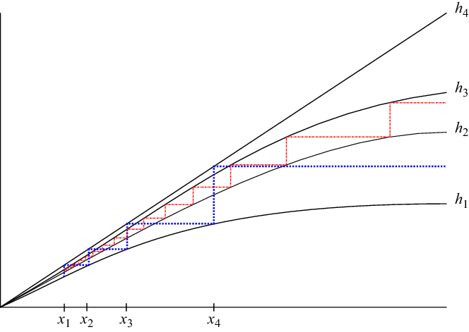
Example 3.4. Suppose we are given functions
 \begin{equation*}h_i \colon [0,\infty) \to [0,\infty),\end{equation*}
where
 $i=1,2,3,4$
satisfying:
-
(i)
$h_i(0)=0$
and
$h_i$
is strictly increasing and continuous for every i, -
(ii)
$h_1<h_2<h_3<h_4$
, -
(iii)
$h_1$
and
$h_2$
are concave.


First we define the sequences
 $(x_n)$
and
 $(y_n)$
by requiring:
-
(i)
$x_0=y_0=1$
, -
(ii)
$x_{n+1}=h_1^{-1}(h_4(x_n))$
, -
(iii)
$y_{n+1}=h_2^{-1}(h_3(x_n))$
,


where
 $n \in \{0,1,2,\ldots\}$
. Then we construct random variables X and Y, whose probability mass is concentrated to the sets
 $\{x_n\colon n\in \mathbb{N}\}$
and
 $\{y_n\colon n\in \mathbb{N}\}$
, respectively. We set
 \begin{equation*}\mathbb{P}(X=x_n)= {\textrm{e}}^{-h_4(x_n)}-{\textrm{e}}^{-h_1(x_n)}\end{equation*}
and
 \begin{equation*}\mathbb{P}(Y=y_n)= {\textrm{e}}^{-h_3(y_n)}-{\textrm{e}}^{-h_2(y_n)}\end{equation*}
for
 $n \in \{0,1,2,\ldots\}$
. The procedure is illustrated in Figure 1.
Illustration of the construction of functions
 $R_X$
(blue, large dashes) and
 $R_Y$
(red, small dashes).

Now, by construction, it must hold that
 \begin{equation}\limsup_{x \to \infty} \dfrac{R_X(x)}{h_4(x)}=\limsup_{x \to \infty} \dfrac{R_Y(x)}{h_3(x)}=\liminf_{x \to \infty} \dfrac{R_Y(x)}{h_2(x)}=\liminf_{x \to \infty} \dfrac{R_X(x)}{h_1(x)}=1.\end{equation}
By continuity of the functions
 $h_i$
, the difference of hazard functions
 $R_X(x)-R_Y(x)$
must change signs infinitely many times. This implies that the tails must also cross infinitely many times. However, from (3.3) we may still conclude that
 $h_1$
is a lower concave approximation of X and
 $h_2$
is a lower concave approximation of Y.
4. Proofs
Proof of Proposition 2.1. We divide the proof into separate cases.
1. We will first prove (2.1). To see that
 \begin{equation*}\mathbb{I}(S_N) \geq \min(\mathbb{I}(N),\mathbb{I}(X)),\end{equation*}
we can use one of the following tools:
-
(i) subadditivity of the function
$x\mapsto x^s$
for
$x\geq 0$
and
$0<s\leq 1$
, -
(ii) Jensen’s inequality, or
-
(iii) Minkowski’s inequality.


Depending on the value of s, the aim is to bound the expectation
 $\mathbb{E}((S_N^+)^s)$
from above. Suppose
 $0<s\leq 1$
. Because of the fact
 $S_N^+\leq \sum_{k=1}^N X_k^+$
and the subadditivity, it must hold that
 \begin{align}\mathbb{E}((S_N^+)^s)&\leq \sum_{k=1}^\infty \,\mathbb{E} \biggl( \biggl( \sum_{m=1}^k X_m^+\biggr)^s \biggr)\,\mathbb{P}(N=k) \notag\\*&\leq \sum_{k=1}^\infty k \,\mathbb{E} ( (X^+)^s)\,\mathbb{P}(N=k)\notag \\*&= \mathbb{E}( (X^+)^s)\,\mathbb{E}(N).\end{align}
On the other hand, applying Jensen’s inequality to the concave function
 $x\mapsto x^s$
, we get
 \begin{align}\mathbb{E}((S_N^+)^s)&\leq \sum_{k=1}^\infty \,\mathbb{E} \biggl( \biggl( \sum_{m=1}^k X_m^+\biggr)^s \biggr)\,\mathbb{P}(N=k) \notag \\*&\leq \sum_{k=1}^\infty k^s(\mathbb{E} ( X^+))^s\,\mathbb{P}(N=k) \notag \\*&= (\mathbb{E} ( X^+))^s\,\mathbb{E}(N^s). \end{align}
Suppose then
 $s>1$
. By Minkowski’s inequality we have
 \begin{align*}\mathbb{E}((S_N^+)^s) \leq \sum_{k=1}^\infty \,\mathbb{E} \biggl( \biggl( \sum_{m=1}^k X_m^+\biggr)^s \biggr)\,\mathbb{P}(N=k) \notag \\& \leq \sum_{k=1}^\infty k^s\,\mathbb{E} ( (X^+)^s)\,\mathbb{P}(N=k)\notag \\ &= \mathbb{E}( (X^+)^s)\,\mathbb{E}(N^s).\end{align*}
Equations (4.1), (4.2), and (4.3) imply
 $\mathbb{I}(S_N) \geq \min(\mathbb{I}(N),\mathbb{I}(X))$
under the assumption that one of the expectations
 $\mathbb{E}(X^+)$
or
 $\mathbb{E}(N)$
is finite.
We will then prove
 $\mathbb{I}(S_N) \leq \min(\mathbb{I}(N),\mathbb{I}(X))$
. Choose m so that
 $\mathbb{P}(N=m)>0$
. Then
 \begin{equation}(S_N)^+\geq (X_1+X_2+\cdots+X_m)^+ \textbf{1}(N=m),\end{equation}
and we have
 $\mathbb{I}(S_N) \leq \mathbb{I}(X_1+X_2+\cdots+X_m)=\mathbb{I}(X)$
by the i.i.d assumption and basic calculation rules of moment indices (see e.g. [Reference Lehtomaa13]). In the case of a finite expectation we note that, for any
 $a\in (0,\mathbb{E}(X))$
, we have
 $\mathbb{P}(S_k>ak)\geq C$
for all k and some
 $C>0$
that does not depend on k. This is clear from the law of large numbers. In the remaining case where
 $\mathbb{E}(|X|)=\infty$
but
 $S_n\to \infty$
almost surely, we have
 $S_n/n\to \infty$
almost surely (see the beginning of e.g. [Reference Kesten and Maller12]). Hence, for
 $a>0$
,
 \begin{align*}\mathbb{E}((S_N^+)^s)& = \sum_{k=1}^\infty \,\mathbb{E} ( ( S_k^+ )^s )\,\mathbb{P}(N=k) \notag \\*&\geq \sum_{k=1}^\infty \,\mathbb{E} ( ( S_k^+)^s \textbf{1}(S_k>ak))\,\mathbb{P}(N=k) \notag \\& \geq a^s\sum_{k=1}^\infty k^s \,\mathbb{P}(S_k>ak)\,\mathbb{P}(N=k) \notag \\*& \geq a^sC\,\mathbb{E}(N^s),\end{align*}
which proves
 $\mathbb{I}(S_N) \leq \mathbb{I}(N)$
. This ends the proof of (2.1).
2. We are set to prove (2.2). Since the proof of the inequality
 $\mathbb{I}(S_N) \leq \min(\mathbb{I}(N),\mathbb{I}(X))$
did not require any assumptions about the finiteness of the expected values
 $\mathbb{E}(|X|)$
and
 $\mathbb{E}(N)$
, we only need to show
 $\mathbb{I}(S_N) \geq \mathbb{I}(X) \mathbb{I}(N).$
Without any loss of generality we can assume that
 $\min(\mathbb{I}(N),\mathbb{I}(X))>0$
.
Recall that
 $\mathbb{E}(X^+)=\infty$
, so
 $\mathbb{I}(X)\leq 1$
. Fix a number
 $\epsilon>0$
so small that for
 $q_1:= \mathbb{I}(X)-\epsilon$
we have
 $q_1>0$
. Set
 $q_2:= \mathbb{I}(N)$
and
 $q:= q_1 q_2$
. Now, for
 $0<s<1$
, it holds by subadditivity and Jensen’s inequality that
 \begin{align}\mathbb{E}(((S_N^+)^q)^s)&\leq \sum_{k=1}^\infty \,\mathbb{E} \biggl( \biggl( \biggl(\sum_{m=1}^k X_m^+\biggr)^{q_1} \biggr)^{q_2s} \biggr)\,\mathbb{P}(N=k) \notag\\*&\leq \sum_{k=1}^\infty \,\mathbb{E} \biggl( \biggl( \sum_{m=1}^k ( X_m^+)^{q_1} \biggr)^{q_2s} \biggr)\,\mathbb{P}(N=k) \notag \\&\leq \sum_{k=1}^\infty k^{q_2s}(\mathbb{E} ( (X^+)^{q_1}))^{q_2s}\,\mathbb{P}(N=k)\notag \\*&= (\mathbb{E} ( (X^+)^{q_1}))^{q_2s}\,\mathbb{E}(N^{q_2s})<\infty.\end{align}
Inequality (4.5) implies
 $\mathbb{I}((S_N^+)^q)\geq 1$
, which is equivalent to
 \begin{equation*}\mathbb{I}(S_N)\geq q=(\mathbb{I}(X)-\epsilon)\mathbb{I}(N).\end{equation*}
Now, letting
 $\epsilon \to 0$
proves the claim.
Proof of Corollary 2.1. Set
 \begin{equation*} S^a_N:= \sum_{k=1}^N ( X_k-\mathbb{E}(X_k)+|\mathbb{E}(X_k)|+1) \end{equation*}
and
 \begin{equation*} S^b_N:= \sum_{k=1}^N ( X_k-\mathbb{E}(X_k)-(|\mathbb{E}(X_k)|+1)). \end{equation*}
Since
 $ S^{b}_N\leq S_N\leq S^a_N$
, it must hold that
 \begin{equation}\mathbb{I}(S^{b}_N) \geq \mathbb{I}(S_N) \geq \mathbb{I}(S^a_N).\end{equation}
The underlying random walk of
 $S^a_N$
is positive, while that of
 $S^b_N$
is negative.
By Proposition 2.1,
 $\mathbb{I}(S^a_N)=\min(\mathbb{I}(X-\mathbb{E}(X)+|\mathbb{E}(X)|+1),\mathbb{I}(N))$
. Using the basic properties of moment indices (see e.g. Section 2.2 of [Reference Lehtomaa13]) and the assumption
 $\mathbb{I}(N)\geq \mathbb{I}(X)$
, we have
 $\mathbb{I}(S^a_N)=\mathbb{I}(X)$
. Moreover, inequality (4.4) holds in this case as well, and we obtain
 $\mathbb{I}(S^{b}_N)\leq \mathbb{I}(X-\mathbb{E}(X)-(|\mathbb{E}(X)|+1))=\mathbb{I}(X)$
. Equation (4.6) proves the claim.
The proof of Proposition 2.1 was based on application of classical inequalities. Once we move on to the study of general scales, the following two technical lemmas become necessary.
Lemma 4.1. Suppose that
 $h \colon [0,\infty) \to [0,\infty)$
is an increasing concave function with
 $h(0)=0$
. Then, for all
 $x\geq 0$
,
 \begin{equation*} \begin{cases} h(cx)\geq ch(x) & {if \ 0<c<1\ and}\\
h(cx)\leq ch(x) & {if\ c>1 .}\end{cases} \end{equation*}
Proof. See Lemma 4 of [Reference Lehtomaa14]
Lemma 4.2. Let X be a non-negative heavy-tailed random variable and let
 $h_X$
be a lower concave approximation of X. Then the mapping
 \begin{equation*}c \mapsto \mathbb{I}_{h_X}(cX) \end{equation*}
is continuous at point
 $c=1$
.
Proof. By concavity and the property
 $h_X(0)=0$
, Lemma 4.1 is applicable.
For a fixed
 $0<c_1<1$
and
 $s\geq 0$
we may estimate
 $\mathbb{E}({\textrm{e}}^{sh_X(c_1X)})\geq \mathbb{E}({\textrm{e}}^{c_1 s h_X(X)})$
and obtain, from connection (1.3), for example, that
 \begin{equation}\sup \{s\geq 0\colon \mathbb{E}({\textrm{e}}^{sh_X(c_1X)})<\infty\} \leq \sup \{s\geq 0\colon \mathbb{E}({\textrm{e}}^{sc_1h_X(X)})<\infty\} =\dfrac{1}{c_1}.\end{equation}
Similarly, for a fixed
 $c_2>1$
we have
 $\mathbb{E}({\textrm{e}}^{sh_X(c_2X)})\leq \mathbb{E}({\textrm{e}}^{c_2 s h_X(X)})$
and so
 \begin{equation}\sup \{s\geq 0\colon \mathbb{E}({\textrm{e}}^{sh_X(c_2X)})<\infty\} \geq \sup \{s\geq 0\colon \mathbb{E}({\textrm{e}}^{sc_2h_X(X)})<\infty\} =\dfrac{1}{c_2}.\end{equation}
Letting
 $c_1\uparrow 1$
in (4.7) and
 $c_2 \downarrow 1$
in (4.8), we finally get that
 \begin{equation*}\lim_{c \to 1} ( \sup \{s\geq 0\colon \mathbb{E}({\textrm{e}}^{sh_X(cX)})<\infty\})= 1, \end{equation*}
which proves the claim.
The following lemma is an extended version of Lemma 3 of [Reference Denisov, Korshunov and Foss5]. It utilises Lemma 4 of [Reference Denisov, Korshunov and Foss5] in its proof.
Lemma 4.3. Suppose
 $\xi,\xi_1,\xi_2,\ldots$
is an i.i.d. sequence of integrable random variables. Let
 $h\colon [0,\infty) \to [0,\infty)$
be an increasing concave function with the property
 $h(x)\geq \log x$
for all x large enough. Assume further that
 $h(x)={\textrm{o}}(x)$
, as
 $x\to \infty$
and
 $\mathbb{E}({\textrm{e}}^{h(\xi^+)})<\infty$
.
Then the following inequalities hold.
-
(a) If
$\mathbb{E}(\xi)=\mu> 0$
, then for every
$c>\mu$
there exists a constant K(c) depending on the distribution of
$\xi$
and the number c, but not on the index n, so that
(4.9)holds for all n.
\begin{equation}\mathbb{E}({\textrm{e}}^{h((\xi_1+\cdots +\xi_n)^+)})\leq K(c) \,{\textrm{e}}^{h(nc)}\end{equation}
-
(b) If
$\mu\leq 0$
, then an inequality corresponding to (4.9) is valid for any
$c>0$
.


Proof. Let the function h be continued to the negative real axis in a concave way. Denote
 $S_n:= \xi_1+\cdots +\xi_n$
. Suppose first that
 $\xi$
has a bounded left tail, i.e.
 $\xi\geq -M$
for some
 $M>0$
. Define
 $a:= \mu/2$
and
 $\eta_n:= \xi_n-c$
so that
 $\mathbb{E}(\eta_n)<0$
.
Now, for any
 $n\in \mathbb{N}$
,
 $c>\mu$
, and
 $b\geq 0$
, it holds that
 \begin{align*}\mathbb{E}({\textrm{e}}^{h(S_n+b)})&= \mathbb{E}({\textrm{e}}^{h(S_{n-1}+b+c+\eta_n)}) \\*&= \mathbb{E}({\textrm{e}}^{h(S_{n-1}+b+c+\eta_n)}\textbf{1}(S_{n-1}\leq a(n-1))) \\*&\quad\, +\mathbb{E}({\textrm{e}}^{h(S_{n-1}+b+c+\eta_n)}\textbf{1}(S_{n-1}> a(n-1))) \\&\leq \mathbb{E}({\textrm{e}}^{h(a(n-1)+b+c+\eta_n)})\,\mathbb{P}(S_{n-1}\leq a(n-1)) \\*&\quad\, +\mathbb{E}({\textrm{e}}^{h(S_{n-1}+b+c+\eta_n)}\textbf{1}(S_{n-1}> a(n-1))).\end{align*}
Let
 $x_0$
be as in Lemma 4 of [Reference Denisov, Korshunov and Foss5] and set
 $n_0:= \lceil x_0/a+1 \rceil$
. Now, for
 $n>n_0$
,
 \begin{equation*}\mathbb{E}({\textrm{e}}^{h(a(n-1)+b+c+\eta_n)})\leq {\textrm{e}}^{h(a(n-1)+b+c)}.\end{equation*}
Furthermore, by the same lemma,
 \begin{equation*}\mathbb{E}({\textrm{e}}^{h(S_{n-1}+b+c+\eta_n)}\textbf{1}(S_{n-1}> a(n-1)))\leq \mathbb{E}({\textrm{e}}^{h(S_{n-1}+b+c)}).\end{equation*}
Hence
 \begin{equation*}\mathbb{E}({\textrm{e}}^{h(S_n+b)})\leq {\textrm{e}}^{h(a(n-1)+b+c)}\,\mathbb{P}(S_{n-1}\leq a(n-1))+\mathbb{E}({\textrm{e}}^{h(S_{n-1}+b+c)}). \end{equation*}
Thus inductive reasoning gives
 \begin{equation}\mathbb{E}({\textrm{e}}^{h(S_n)})\leq {\textrm{e}}^{h(cn)}\sum_{k=n_0}^{\infty} \,\mathbb{P}(S_{k}\leq ak)+\mathbb{E}({\textrm{e}}^{h(S_{n_0}+nc)}).\end{equation}
The series on the right-hand side of (4.10) converges because probabilities
 $\mathbb{P}(S_{k}\leq ak)$
decay at an exponential rate due to the fact that they are bounded from below and
 $a<\mu$
. So, there is a constant N(c) such that
 \begin{equation}\mathbb{E}({\textrm{e}}^{h(S_n)})\leq N(c)\,{\textrm{e}}^{h(cn)}.\end{equation}
In order to show (4.9), it suffices to note that
 \begin{equation*}\mathbb{E}({\textrm{e}}^{h((S_n)^+)})\leq {\textrm{e}}^{h(0)}+\mathbb{E}({\textrm{e}}^{h(S_n)})\end{equation*}
and use (4.11).
For part it remains to consider the situation where
 $\xi$
has an unbounded left tail. Select
 $M_1>0$
so that
 \begin{equation*}|\mathbb{E}(\xi\textbf{1}(\xi<-M_1))|<(c-\mu)/2. \end{equation*}
Then
 \begin{equation*}\hat{\xi}:= \xi\textbf{1}(\xi\geq -M_1)\end{equation*}
satisfies
 $\mathbb{E}(\hat{\xi})\eqcolon \hat{\mu}\in (\mu,(\mu+c)/2)$
. Now
 $\hat{\xi}$
has a bounded left tail and therefore the previous proof can be applied. Denote
 $\hat{S}_n:= \hat{\xi}_1+\cdots+\hat{\xi}_n$
to get
 \begin{equation*}\mathbb{E}({\textrm{e}}^{h((S_n)^+)})\leq \mathbb{E}({\textrm{e}}^{h((\hat{S}_n)^+)})\leq K(c) \,{\textrm{e}}^{h(n c)},\end{equation*}
as required.
To show case , one can estimate
 $\xi\leq \xi-\mu+c/2$
and apply part to a random variable
 $\hat{\xi}:= \xi-\mu+c/2$
with
 $\mathbb{E}(\hat{\xi})=c/2$
, where
 $c>0$
is arbitrary.
Proof of Theorem 2.1. 1. Recall that
 $c_1$
is a finite constant such that
 $c_1>\mu>0$
. Note first that assumption (2.3) implies
 \begin{equation*}\liminf_{x \to \infty} \dfrac{R_{c_1N}(x)}{h_X(x)} \geq \biggl( \liminf_{x \to \infty} \dfrac{R_{c_1N}(x)}{h_N(x/c_1)}\biggr) \biggl( \liminf_{x \to \infty} \dfrac{h_N(x/c_1)}{h_X(x)}\biggr)\geq 1.\end{equation*}
Using part of Lemma 1.2, we see that
 \begin{equation}\mathbb{E}({\textrm{e}}^{(1-\epsilon)h_X(c_1N)})<\infty\end{equation}
for any
 $\epsilon>0$
.
Recall from assumptions that
 $\delta>0$
is fixed. Set
 \begin{equation*}0<\eta<\delta/(1+\delta).\end{equation*}
Using the fact that
 \begin{equation*}(1-\eta)h_X(x)\geq \log x\end{equation*}
for large enough x and that Lemma 4.3 is applicable by definitions, we obtain the upper bound
 \begin{equation}\mathbb{E}({\textrm{e}}^{(1-\eta)h_X(S_n^+)})\leq K(c_1)\,{\textrm{e}}^{(1-\eta)h_X(c_1 n)}\end{equation}
for all
 $n \in \mathbb{N}$
, where the constant
 $K(c_1)$
only depends on
 $c_1$
but not on n. Utilising estimates (4.13) and (4.12), we get by (4.12)
 \begin{align*}\mathbb{E}({\textrm{e}}^{(1-\eta)h_X(S_N^+)})&=\sum_{k=1}^\infty \,\mathbb{E}({\textrm{e}}^{(1-\eta)h_X(S_k^+)})\,\mathbb{P}(N=k) \\*&\leq \sum_{k=1}^\infty K(c_1)\,{\textrm{e}}^{(1-\eta)h_X(c_1 k)} \,\mathbb{P}(N=k) \\*&= K(c_1)\,\mathbb{E}({\textrm{e}}^{(1-\eta)h_X(c_1 N)})<\infty.\end{align*}
Since the mapping
 $s \mapsto \mathbb{E}({\textrm{e}}^{sh_X(S_N^+)})$
is increasing,
 $\mathbb{E}({\textrm{e}}^{sh_X(S_N^+)})<\infty$
holds for all
 $0<s<1$
. Thus
 $\mathbb{I}_{h_X}(S_N)\geq 1$
. On the other hand, for any
 $\epsilon>0$
it holds that
 \begin{equation*}\mathbb{E}({\textrm{e}}^{(1+\epsilon)h_X(S_N^+)})\geq \mathbb{E}({\textrm{e}}^{(1+\epsilon)h_X(X^+)})\,\mathbb{P}(N=m)\,\mathbb{P}(X\geq 0)^{m-1}=\infty \end{equation*}
for some m and so
 $\mathbb{I}_{h_X}(S_N)\leq 1$
. This proves that
 $\mathbb{I}_{h_X}(S_N)= 1$
and so
 $h_X$
is a lower concave approximation of
 $S_N$
.
2. Suppose
 $0<\eta_1<\delta/(1+\delta)$
is fixed and denote
 $\mathbb{E}(X)=\mu$
. Fix the version of lower concave approximation of
 $\mu N$
by setting
 $h_{\mu N}(x):= h_N(x/\mu)$
. The mapping
 $c\mapsto \mathbb{I}_{h_{\mu N}}(cN)$
is continuous in a neighbourhood of
 $\mu$
, because by Lemma 1.1
 $\mathbb{I}_{h_{\mu N}}(cN)=\mathbb{I}_{h_{N}}((c/\mu)N)$
, and the latter is continuous at point 1 by Lemma 4.2.
Set
 $g(x)=h_N(\mu/x)$
. Since
 $\mathbb{E}({\textrm{e}}^{(1-\eta_1)h_N(N)})<\infty$
for all
 $\eta_1\in(0,1)$
, it holds that
 $1-\eta_1<\mathbb{I}_g(\mu N)$
. In particular, by continuity we may find a number
 $c_{\eta_1}>\mu$
satisfying
 $1-\eta_1<\mathbb{I}_g(c_{\eta_1}N)$
so that
 \begin{equation}\mathbb{E}({\textrm{e}}^{(1-\eta_1)h_{\mu N}(c_{\eta_1} N)})<\infty.\end{equation}
Furthermore, we get
 \begin{equation*}\liminf_{x \to \infty} \dfrac{R_{X}(x)}{h_{\mu N}(x)} \geq \biggl( \liminf_{x \to \infty} \dfrac{R_{X}(x)}{h_X(x)}\biggr) \biggl( \liminf_{x \to \infty} \dfrac{h_X(x)}{h_{N}(x/\mu )}\biggr)\geq 1\end{equation*}
from assumption (2.4) and thus
 $\mathbb{I}_g(X)\geq 1$
, so that
 \begin{equation*} \mathbb{E}({\textrm{e}}^{(1-\eta_1)h_{\mu N}(X)})<\infty.\end{equation*}
In addition,
 \begin{equation*}(1-\eta_1)h_{\mu N}(x)=(1-\eta_1)h_{N}(x/\mu ) \geq \log x\end{equation*}
for large enough x by the choice of
 $\eta_1$
. This makes Lemma 4.3 applicable. Using arguments similar to those in part of the theorem and equation (4.14), we obtain
 \begin{align*}\mathbb{E}({\textrm{e}}^{(1-\eta_1)h_{\mu N}(S_N^+)})&=\sum_{k=1}^\infty \,\mathbb{E}({\textrm{e}}^{(1-\eta_1)h_{\mu N}(S_k^+)})\,\mathbb{P}(N=k) \\*&\leq \sum_{k=1}^\infty K(c_{\eta_1})\,{\textrm{e}}^{(1-\eta_1)h_{\mu N}(c_{\eta_1} k)} \,\mathbb{P}(N=k) \\*&= K(c_{\eta_1})\,\mathbb{E}({\textrm{e}}^{(1-\eta_1)h_{\mu N}(c_{\eta_1} N)})<\infty.\end{align*}
This shows
 $\mathbb{I}_{h_{\mu N}}(S_N)\geq 1.$
The other direction follows from the law of large numbers. Assume
 $\eta_2>0$
is given. Then by Lemma 4.2 we may choose a number
 $0<c_{\eta_2}<\mu$
so that
 \begin{equation*} \mathbb{E}({\textrm{e}}^{(1+\eta_2)h_{\mu N}(c_{\eta_2} N)})=\infty.\end{equation*}
In addition, by the law of large numbers we may find a constant
 $C=C_{\eta_2,c_{\eta_2}}>0$
such that
 $\mathbb{P}(S_k>c_{\eta_2} k)\geq C$
for all
 $k \in \mathbb{N}$
. Now
 \begin{align*}\mathbb{E}({\textrm{e}}^{(1+\eta_2)h_{\mu N}(S_N^+)})&= \sum_{k=1}^\infty \,\mathbb{E}({\textrm{e}}^{(1+\eta_2)h_{\mu N}(S_k^+)})\,\mathbb{P}(N=k) \\*& \geq \sum_{k=1}^\infty \,\mathbb{E}({\textrm{e}}^{(1+\eta_2)h_{\mu N}(S_k^+)}\textbf{1}(S_k>c_{\eta_2} k))\,\mathbb{P}(N=k) \\&= \sum_{k=1}^\infty \,{\textrm{e}}^{(1+\eta_2)h_{\mu N}(c_{\eta_2} k)}\,\mathbb{P}(S_k>c_{\eta_2} k)\,\mathbb{P}(N=k) \\& \geq C\sum_{k=1}^\infty \,{\textrm{e}}^{(1+\eta_2)h_{\mu N}(c_{\eta_2} k)}\,\mathbb{P}(N=k) \\*&= C \,\mathbb{E}({\textrm{e}}^{(1+\eta_2)h_{\mu N}(c_{\eta_2} N)})=\infty.\end{align*}
This proves
 $\mathbb{I}_{h_{\mu N}}(S_N)\leq 1$
and we get
 $\mathbb{I}_{h_{\mu N}}(S_N)= 1$
, so
 $h_N(x/\mu)$
is a lower concave approximation of
 $S_N$
.
Remark 4.1. As was kindly pointed out by a reviewer, some of the steps in the proof of Theorem 2.1 admit shorter alternative justifications based on well-known inequalities in the case where the increment dominates the number of claims. This is specifically true if it is assumed, in addition to the assumptions made, that the increments belong to the strongly subexponential class of heavy-tailed variables or that the increments can be stochastically bounded by variables of such a class. In more detail, if increment
 $X_1$
can be stochastically bounded by variable
 $Y_1$
whose tail function is of the form
 ${\textrm{e}}^{-(1-\epsilon)h_X(x)}$
for large enough x, it follows from Theorem 3.30 of [Reference Foss, Korshunov and Zachary8] that the distribution of
 $Y_1$
is strongly subexponential and consequently the known results for this distribution class become available for the estimates.
Proof of Corollary 2.2. Note first that
 $\mathbb{P}(S_N>x)\geq \mathbb{P}(X>x)$
and therefore
 $R_{S_N}(x)\leq R_X(x)$
holds for all x, since
 $X\geq 0$
almost surely. Application of Theorem 2.1 and assumption (2.5) gives
 \begin{equation*}1=\liminf_{x\to \infty} \dfrac{R_{S_N}(x)}{h_X(x)}\leq \limsup_{x\to \infty} \dfrac{R_{S_N}(x)}{h_X(x)}\leq \limsup_{x\to \infty} \dfrac{R_{X}(x)}{h_X(x)}=1 \end{equation*}
and proves the claim. The proof of the remaining case is similar.
Proof of Lemma 2.1. The implication is verified by observing that (2.8), together with the definition of lower concave approximation and positivity, yields
 \begin{equation*}\liminf_{x \to \infty} \dfrac{R(x)}{\sqrt{x}}\geq \biggl( \liminf_{x \to \infty} \dfrac{h(x)}{\sqrt{x}} \biggr) \biggl(\liminf_{x \to \infty} \dfrac{R(x)}{h(x)}\biggr) >0.\end{equation*}
Hence, by part of Lemma 1.1, there exists
 $c>0$
such that
 \begin{equation*}\mathbb{E}( {\textrm{e}}^{c\sqrt{X}})<\infty ,\end{equation*}
and Theorem 1 of [Reference Stoyanov and Lin23] confirms that X is determined by its moments.
Proof of Theorem 2.2. The proof utilises techniques similar to those of the proof of Theorem 2.1.
1. Suppose first that condition of Theorem 2.2 holds. Recall that
 $c_1>\mathbb{E}(X)>0$
and
 $X\geq 0$
. Since
 \begin{equation*}\liminf_{x \to \infty} \dfrac{R_{c_1N}(x)}{h_X(x)} \geq \biggl( \liminf_{x \to \infty} \dfrac{R_{c_1N}(x)}{h_N(x/c_1)}\biggr) \biggl( \liminf_{x \to \infty} \dfrac{h_N(x/c_1)}{h_X(x)}\biggr)>0,\end{equation*}
there must exist
 $\eta>0$
so that
 \begin{equation*}\mathbb{E}({\textrm{e}}^{\eta h_X(c_1N)})<\infty. \end{equation*}
Clearly, by assumption (2.9),
 $\eta h_X(x)\geq \log x$
holds for all large enough x. This enables the use of Lemma 4.3. We get
 \begin{align*}\mathbb{E}({\textrm{e}}^{\eta h_X(S_N)})&= \sum_{k=1}^\infty \,\mathbb{E}({\textrm{e}}^{\eta h_X(S_k)})\,\mathbb{P}(N=k) \\*&\leq \sum_{k=1}^\infty K(c_1)\,{\textrm{e}}^{\eta h_X(c_1 k)} \,\mathbb{P}(N=k) \\*&= K(c_1)\,\mathbb{E}({\textrm{e}}^{\eta h_X(c_1 N)})<\infty.\end{align*}
Hence
 $\mathbb{I}_{h_X}(S_N)\geq \eta>0$
. This implies, using part of Lemma 1.1, that
 \begin{equation}\liminf_{x \to \infty} \dfrac{R_{S_N}(x)}{h_X(x)}>0.\end{equation}
By assumption (2.9) there exists a constant
 $c>0$
such that
 $h_X(x)\geq c \sqrt{x}$
for all x large enough. Now (4.15) implies
 \begin{equation*}\liminf_{x \to \infty} \dfrac{R_{S_N}(x)}{\sqrt{x}}>0. \end{equation*}
Hence
 $\sqrt{S_N}$
is light-tailed, and by Hardy’s criterion
 $S_N$
is determined by its moments.
2. The proof of part follows the same kind of arguments as part . First we see that
 \begin{equation*}\liminf_{x \to \infty} \dfrac{R_{X}(x)}{h_{N}(x/\mu)} \geq \biggl( \liminf_{x \to \infty} \dfrac{R_{X}(x)}{h_X(x)}\biggr) \biggl( \liminf_{x \to \infty} \dfrac{h_X(x)}{h_{ N}(x/\mu)}\biggr)>0,\end{equation*}
ensuring the existence of small
 $\eta>0$
so that
 \begin{equation*}\mathbb{E}({\textrm{e}}^{\eta h_{N}(X/\mu)})<\infty. \end{equation*}
Using Lemma 4.2 we may find a constant
 $c_\eta>\mu$
such that we also have
 \begin{equation*}\mathbb{E}({\textrm{e}}^{\eta h_{N}(c_\eta N/\mu)})<\infty .\end{equation*}
Now, again, by Lemma 4.3 we get
 \begin{align*}\mathbb{E}({\textrm{e}}^{\eta h_{N}(S_N/\mu)})&= \sum_{k=1}^\infty \,\mathbb{E}({\textrm{e}}^{\eta h_{N}(S_k/\mu)})\,\mathbb{P}(N=k)\\*&\leq \sum_{k=1}^\infty K(c_\eta)\,{\textrm{e}}^{\eta h_{N}(c_\eta k/\mu)} \,\mathbb{P}(N=k) \\*&= K(c_1)\,\mathbb{E}({\textrm{e}}^{\eta h_{N}(c_\eta N/\mu)})<\infty.\end{align*}
The conclusion follows in the same way as for part .
Appendix A. Technical details
Technical details omitted during the main text are presented here.
A.1 Part (d) of Lemma 1.2
Proof of Lemma 1.1 part : inequality
 $f_1\geq h_X$
. Proof of the first assertion can be justified using Theorem 2.10 of [Reference Foss, Korshunov and Zachary8]. Let g be a non-negative, strictly increasing, and continuous function for which
 $g(x)={\textrm{o}}(R(x))$
and
 $g(x)\to \infty$
, as
 $x \to \infty$
. Thus, by part of Lemma 1.1 it holds that
 \begin{equation}\sup\{s\geq 0\colon \mathbb{E}({\textrm{e}}^{ s g(X)})<\infty\}=\liminf_{x \to \infty} \dfrac{ R(x)}{g(x)}=\infty.\end{equation}
Application of Theorem 2.10 of [Reference Foss, Korshunov and Zachary8] shows that there exists a concave function, say
 $\hat{h}$
, satisfying
 $\hat{h}\leq f_1$
,
 \begin{equation}\mathbb{E}({\textrm{e}}^{\hat{h}(X)})<\infty\end{equation}
and
 \begin{equation}\mathbb{E}({\textrm{e}}^{\hat{h}(X)+g(X)})=\infty.\end{equation}
Without loss of generality we may additionally assume
 $\hat{h}(0)=0$
.
Now, for any
 $\epsilon\in (0,1)$
, it holds that
 \begin{equation*} \mathbb{E}({\textrm{e}}^{(1-\epsilon)\hat{h}(X)})<\infty\end{equation*}
due to (A.2). It must also hold that
 \begin{equation}\mathbb{E}({\textrm{e}}^{(1+\epsilon)\hat{h}(X)})=\infty.\end{equation}
If (A.4) were violated, (A.1) and Hölder’s inequality for
 $1/p+1/q=1$
, where
 $p=1+\epsilon$
, would imply
 \begin{equation*}\mathbb{E}({\textrm{e}}^{\hat{h}(X)+g(X)})\leq \mathbb{E}({\textrm{e}}^{(1+\epsilon)\hat{h}(X)})^{1/(1+\epsilon)}\,\mathbb{E}({\textrm{e}}^{q g(X)})^{1/q} <\infty\end{equation*}
contradicting (A.3). Thus we may choose
 $h_X=\hat{h}$
.
Proof of Lemma 1.1 part : inequality
 $h_X^*\geq f_2$
. If
 $\sup\{ s\geq 0\colon \mathbb{E}({\textrm{e}}^{sf_2(X)})<\infty\}\eqcolon \alpha\in [1,\infty), $
one can take
 $h_X^*(x)=\alpha f_2(x)$
.
Suppose that
 $\sup\{ s\geq 0\colon \mathbb{E}({\textrm{e}}^{sf_2(X)})<\infty\}=\infty. $
Now part of Lemma 1.1 implies
 \begin{equation*}\lim_{x \to \infty} \dfrac{ R(x)}{f_2(x)}=\infty.\end{equation*}
Specifically,
 $2f_2(x)={\textrm{o}}(R(x))$
, as
 $x\to \infty$
.
Let h be some lower concave approximation of X with
 $h(0)=0$
. Clearly
 \begin{equation*}\liminf_{x \to \infty} \dfrac{R(x)}{h(x)+2f_2(x)}\leq \liminf_{x \to \infty} \dfrac{R(x)}{h(x)} =1.\end{equation*}
On the other hand, for any x large enough,
 $2f_2(x)/R(x)\leq 1$
holds. Hence
 \begin{align*}\liminf_{x \to \infty} \dfrac{R(x)}{h(x)+2f_2(x)} &= \liminf_{x \to \infty} \dfrac{1}{h(x)/R(x)+2f_2(x)/R(x)}\\*&\geq \liminf_{x \to \infty} \dfrac{1}{h(x)/R(x)+1} \\&= \liminf_{x \to \infty} \dfrac{R(x)}{h(x)+R(x)} \\&\geq \dfrac{1}{2} \liminf_{x \to \infty} \dfrac{R(x)}{\max(h(x),R(x))} \\&=\dfrac{1}{2} \liminf_{x \to \infty} \dfrac{1}{\max(h(x)/R(x),1)} \\*&=\dfrac{1}{2} \liminf_{x \to \infty} \biggl( \min \biggl( \dfrac{R(x)}{h(x)},1 \biggr) \biggr) =\dfrac{1}{2},\end{align*}
that is,
 \begin{equation*}\liminf_{x \to \infty} \dfrac{R(x)}{h(x)+2f_2(x)}\eqcolon c\in [1/2,1].\end{equation*}
In summary:
-
(i)
\begin{equation*}\liminf_{x \to \infty} \dfrac{R(x)}{c(h(x)+2f_2(x))}=1,\end{equation*}
-
(ii)
$c(h(x)+2f_2(x))=0$
, -
(iii)
$c(h(x)+2f_2(x))$
is concave as a sum of two concave functions, -
(iv)
$c(h(x)+2f_2(x))\geq 2cf_2(x)\geq f_2(x).$


Since properties – hold, setting
 $h_X^*(x):= c(h(x)+2f_2(x))$
proves the claim.
A.2 Light-tailed versus heavy-tailed: details for Remark 2.2
Additional results can be obtained in a straightforward way if the assumptions of Theorem 2.1 are modified.
-
(i) Suppose N is light-tailed and X is heavy-tailed. Then the result of Theorem 2.1 part holds when assumption (2.3) is omitted. The proof of the result simplifies substantially compared to the case where both of the variables are heavy-tailed.
Firstly, since N is light-tailed, we have
$\mathbb{E}({\textrm{e}}^{cN})<\infty$
for some
$c>0$
. Thus, by Lemma 1.1 part and the fact that
$h_X(x)={\textrm{o}}(x)$
:
\begin{equation*}\liminf_{x \to \infty} \dfrac{R_{c_1N}(x)}{h_X(x)} \geq \biggl( \liminf_{x \to \infty} \dfrac{R_{c_1N}(x)}{x}\biggr) \biggl( \liminf_{x \to \infty} \dfrac{x}{h_X(x)}\biggr)=\infty.\end{equation*}
This confirms that (4.12) holds, and the rest of the proof is similar to the heavy-tailed case.
-
(ii) Suppose X is light-tailed and N is heavy-tailed. Then a modification similar to that in the first part yields the result without assumption (2.4) of Theorem 2.1 part .


Acknowledgements
The deepest gratitude is expressed to the Finnish Doctoral Programme in Stochastics and Statistics (FDPSS) and the Centre of Excellence in Computational Inference (COIN) for financial support (Academy of Finland grant number 251170). Special thanks are due to Harri Nyrhinen for supportive discussions. The author is thankful to Sø ren Asmussen and Aarhus University for hospitality at the finalisation stage of the paper. Comments made by anonymous reviewers helped to improve the manuscript substantially.