2. THE ARCH MODEL

Assume that we have observed (y_t,x_t−1)_t=1,…,n with

given by the ARCH model,

with parameter

and where x₀ is fixed.

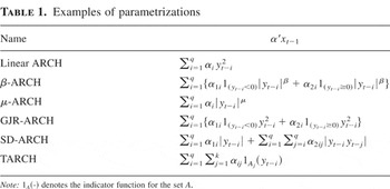
Some of the parametrizations that fall within our framework are given in Table 1: linear ARCH (Engle, 1982), β-ARCH (Guegan and Diebolt, 1994) for known β > 0, μ-ARCH (Engle and Bollerslev, 1986) for known μ > 0, threshold or GJR-ARCH (Glosten et al., 1993; Li and Li, 1996; Zakoian, 1994), SD-ARCH (Schwert, 1990), and TARCH (Gourieroux and Monfort, 1992).

Examples of parametrizations

For the asymptotic analysis, we assume that for θ at the true value θ₀ there exists a stationary solution to equations (1)–(2) and denote this {(y_t*,x_t−1*)}. However, the process {(y_t,x_t−1)} may be nonstationary as x₀, and hence y₁, need not be initiated from the stationary distribution. To emphasize this, in the following discussion let h_0t = ω₀ + α₀′x_t−1 and h_0t* = ω₀ + α₀′x_t−1* denote the true conditional variance process corresponding to {(y_t,x_t−1)} and {(y_t*,x_t−1*)}, respectively. Correspondingly, write h_t = ω + α′x_t−1 and h_t* for any θ ≠ θ₀.

The following conditions are assumed to hold.

C.1. The innovations {z_t} are i.i.d.(0,1) with E [|log(z_t²)|] < ∞.

C.2. The parameter space is given by

for some fixed ω > 0.

C.3. For all t ≥ 1, (i) x_i,t−1 ≥ 0, 1 ≤ i ≤ m, (ii) x_t−1 is measurable w.r.t.

for some finite q ≥ 1, and (iii) P(β′x_t−1* ≠ c) > 0 for any

.

C.4. (i) {(y_t,x_t−1)} is geometrically ergodic such that for the true parameter θ₀ ∈ Θ a stationary solution {(y_t*,x_t−1*)} exists with (ii) E [|log(x_i,t*)|] < ∞, 1 ≤ i ≤ m.

The assumptions made in C.1 about the rescaled errors are fairly standard, where we note that the i.i.d. assumption is needed to obtain the Markov property of {(y_t,x_t−1)}. Lee and Hansen (1994) assumed that {z_t} was a stationary martingale difference sequence. It is possible here to introduce limited dependence in the {z_t} process without removing the Markov property, e.g., by assuming that {(z_t,…,z_t−p)} is a geometrically ergodic Markov chain for some finite p ≥ 0 and satisfying

where

includes the lagged z_t's too. For simplicity, we maintain the i.i.d. assumption however.

Condition C.2 defines the noncompact parameter space Θ for the statistical analysis; i.e., the quasi-likelihood function defined subsequently is maximized over θ ∈ Θ. Condition C.2 implies—together with C.3(i) and (ii)—that h_t > 0 for all θ ∈ Θ.

Note that the only real restriction on the parameter space Θ is the requirement that the constant term, ω, is bounded from below by some ω > 0. It is used when deriving a uniform lower bound for the quasi-likelihood function in the proof of Lemma 4 and appears difficult to avoid.

For the asymptotics, or the probability analysis, condition C.4(i) of geometric ergodicity restricts the possible values of the true value θ₀ in Θ. As noted geometric ergodicity implies that the strong LLN holds for {(y_t,x_t−1)} irrespective of initial values. Explicit conditions for which C.4 holds in some leading examples are given in Section 5, Theorem 3 and Corollary 1. The assumption of geometric ergodicity can be exchanged with the weaker condition that there exists a version of {(y_t,x_t−1)} that is stationary and ergodic. But then one needs to either (i) assume that it is the stationary version that has been observed (see Jeantheau, 1998) or (ii) show that the observed quasi-likelihood function converges uniformly toward the stationary version of it (see Lee and Hansen, 1994).

Condition C.3(iii) is a nondegeneracy condition that is used in the proof of identification of θ₀. A sufficient, but stronger, condition for C.3(iii) would be that E [x_t−1*x_t−1*′] is nonsingular, which however requires that the moment exists. For example, in the linear ARCH model we would have to require that E [y_t*⁴] < ∞, contradicting empirical findings.

Finally note that it can be shown that a simple condition for the moment in C.4(ii) to exist is E [∥x_t*∥^p] < ∞ for some p > 0. And if one assumes that Θ is compact, the log-moment condition in C.1 can be removed and C.4(ii) weakened to E [|log(h_0t*)|] < ∞; cf. the proof of Lemma 4.

3. CONSISTENCY OF THE QMLE

Our first main result is that the QMLE

is strongly consistent, where

Here

We furthermore define the moment function

which takes values on the extended real line

. This is well defined by Lemma 1. To allow for noncompact Θ when proving consistency, we use the strategy of Huber (1967). The idea is to find a compact set

, as defined in (B.2) in Appendix B, for which

and such that

for some ε > 0. It then follows that

, and we can apply a consistency result of Pfanzagl (1969) on the compact set

. This involves showing that L(θ) is well defined, that θ₀ is identified by L(θ), and that θ [map ] L(θ) is continuous.

THEOREM 1. Under C.1–C.4, the QMLE defined by (3) satisfies

.

4. ASYMPTOTIC NORMALITY OF THE QMLE

In this section we show that the QMLE is asymptotically Gaussian. To prove this result, we impose the following assumptions in addition to C.1–C.4.

N.1. For θ₀ = (ω₀,α₀), ω₀ > ω and α_0,i > 0 for i = 1,…,m.

N.2. κ₄ = E [(z_t² − 1)²] ∈ (0,∞).

Assumption N.1, or equivalently θ₀ ∈ intΘ, is needed for a Taylor expansion of the quasi-likelihood function around θ₀. The case of no ARCH, α₀ = 0, is not straightforward (see, e.g., Andrews, 1999) and will be left for future work. The second condition, N.2, ensures that the asymptotic variance of the QMLE exists.

The proof of asymptotic normality is standard (see, e.g., Basawa, Feigin, and Heyde, 1976), based on a Taylor expansion of the score,

around θ₀. In particular, we show in Lemma 9 that

where

and furthermore in Lemma 8 that uniformly over θ in a compact set containing θ₀,

THEOREM 2. Under C.1–C.4 and N.1 and N.2,

where V(θ₀) and H(θ₀) are given in (6) and (7), both are positive definite. Furthermore,

are strongly consistent estimators of V(θ₀) and H(θ₀), respectively.

Remark 1. In the case where z_t ∼ N(0,1), the result collapses to the standard maximum likelihood estimator (MLE) result with κ₄ = 2 and H(θ₀) being the information matrix multiplied by 2.

5. EXAMPLES

In this section we consider the models shown in Table 1 and demonstrate that under suitable conditions they satisfy C.2–C.4, which are the only assumptions made on the actual parametrization. The remaining assumptions concern the error structure (C.1 and N.2) and the location of θ₀ in the parameter space (C.2 and N.1).

To do so we consider a specific subclass of models of (1)–(2) given by

which contains the models in Table 1 as special cases, except the SD-ARCH because of the cross-product terms. This is treated separately as part of Corollary 1, which follows. In (10),

such that the dimension of x_t−1 is m = qp. For this class, we address the two questions, identification, C.3, and geometric ergodicity, C.4, in turn. Specifically, we make the following assumptions about g.

G.1.

is measurable, j = 1,…,p.

G.2. For any

.

G.3. There exist constants a₀⁽ⁱ⁾ > 0, a₁⁽ⁱ⁾ ≥ 0, i = 1,…,q, with

, such that for

as |y| → ∞.

Note that by Lemma 10, G.1 and G.2 imply C.3. The proof exploits that as y_t−i = h_t−i^1/2z_t−i, G.2 can be seen as a conditional (on h_t−i^1/2 = h) version of C.3(iii) when x_t−1 takes the form (11). The condition G.3 implies that C.4 holds by using the so-called drift criterion from Markov chain theory.

THEOREM 3. Assume (i) that C.1, C.2, N.1, and N.2 hold with z_t ∼ f_z·λ, where f_z > 0 is a lower semicontinuous density w.r.t. the Lebesgue measure λ. Assume further (ii) that α′x_t−1 is given by (10) and that G.1–G.3 hold. Then the QMLE is strongly consistent and asymptotically Gaussian.

As a corollary we state the results specifically for the models in Table 1.

COROLLARY 1. Assume that the assumptions of Theorem 3 hold. Assume further at the true parameter value for the linear ARCH(q), Σ_i=1^qα_0,i < 1; for the β-ARCH, β ∈ (0,2); for the μ-ARCH, μ ∈ (0,2); for the GJR-ARCH, Σ_i=1^q{α_0,1i + α_0,2i} < 1; for the SD-ARCH, Σ_i=1^qα_0,2ii + 2Σ_i=1^qΣ_j=i+1^qα_0,2ij < 1; and for the TARCH,

. Then the QMLE for each model is strongly consistent and asymptotically Gaussian.

Remark 2. Apart from the TARCH case, the last conditions in Corollary 1 are only needed to establish geometric ergodicity. So if weaker conditions for this property can be found, then under these conditions the results remain valid. For example, in the linear ARCH(1) model, we may weaken the preceding condition, α₀ = α_0,1 < 1, to log(α₀) < −E [log(z_t²)] (see Lemma 11). Note that this condition is necessary and sufficient for stationarity and ergodicity (see Nelson, 1990).

Remark 3. The condition given for the TARCH model is used to establish identification. It might be possible to find weaker conditions for this property to hold.