2 The formulation and analytical solutions

Consider a steady SP flow. The vorticity transport equation gives the governing equation

(2.1)$$\begin{eqnarray}\unicode[STIX]{x1D6FB}^{4}\unicode[STIX]{x1D713}=\frac{\unicode[STIX]{x2202}\unicode[STIX]{x1D713}}{\unicode[STIX]{x2202}y}\frac{\unicode[STIX]{x2202}\unicode[STIX]{x1D6FB}^{2}\unicode[STIX]{x1D713}}{\unicode[STIX]{x2202}x}-\frac{\unicode[STIX]{x2202}\unicode[STIX]{x1D713}}{\unicode[STIX]{x2202}x}\frac{\unicode[STIX]{x2202}\unicode[STIX]{x1D6FB}^{2}\unicode[STIX]{x1D713}}{\unicode[STIX]{x2202}y},\end{eqnarray}$$

in which $(x,y)$ are the independent variables in respectively the $x$- and $y$-directions of Cartesian coordinates and $\unicode[STIX]{x1D713}(x,y)$ is the streamfunction; they have been non-dimensionalized respectively by $\sqrt{\unicode[STIX]{x1D708}/\unicode[STIX]{x1D70F}}$ and $\unicode[STIX]{x1D708}$. Note please that $\unicode[STIX]{x1D708}$ is the kinematic viscosity of the fluid and $\unicode[STIX]{x1D70F}$ is a parameter having the units of inverse time. Since the flow impinges obliquely upon the moving boundary at the bottom, the dimensionless boundary conditions are given by

(2.2a-c)$$\begin{eqnarray}\unicode[STIX]{x1D713}(x,0)=0,\quad \frac{\unicode[STIX]{x2202}\unicode[STIX]{x1D713}(x,0)}{\unicode[STIX]{x2202}y}=U,\quad \unicode[STIX]{x1D713}(x,y)\sim \frac{1}{2}y^{2}\cos \unicode[STIX]{x1D6FC}+xy\sin \unicode[STIX]{x1D6FC}\quad \text{as}~y\rightarrow \infty ,\end{eqnarray}$$

in which $U$ is the plate velocity and $\unicode[STIX]{x1D6FC}$ is the impinging angle between the dividing streamline and the plate. Equations (2.2a,b) account for the no-slip boundary condition on the moving plate at $y=0$ and (2.2c) describes the oblique flow at infinite far field.

It was shown by Dorrepaal (Reference Dorrepaal1986) that a similarity solution for such a flow is

(2.3)$$\begin{eqnarray}\unicode[STIX]{x1D713}(x,y)=g(y)+xf(y),\end{eqnarray}$$

where $f(y)$ corresponds to the normal component and $g(y)$ to the tangential component of the flow. Both components shall satisfy the boundary conditions (2.2a,b) at the plate and (2.2c) at infinity. By substituting (2.3) into (2.1) and (2.2a–c), we obtain two sets of equations corresponding to respectively $f(y)$ and $g(y)$. These equations are solved with a mathematical approach proposed by Dorrepaal, which is a combination of analytical derivation and numerical computation. For the details of the mathematical approach, the reader is referred to Cheng (Reference Cheng2019). The solutions of $f(y)$ and $g(y)$ are shown in the following.

For the solution of the normal component, for small $y$ we have

(2.4)$$\begin{eqnarray}f(y)={\textstyle \frac{1}{2}}Ka^{3}y^{2}-{\textstyle \frac{1}{6}}a^{4}y^{3}+O(y^{5});\end{eqnarray}$$

for large $y$ we have

(2.5)$$\begin{eqnarray}\displaystyle f(y) & = & \displaystyle a\left\{ay-A+\exp \left[-{\textstyle \frac{1}{2}}(ay-A)^{2}\right]\right.\nonumber\\ \displaystyle & & \displaystyle \times \left.[-0.01609+0.0568(ay-A)^{-1}-0.000448(ay-A)^{-4}]\vphantom{\left[-{\textstyle \frac{1}{2}}(ay-A)^{2}\right]}\right\}\!.\end{eqnarray}$$

In (2.4) and (2.5), we have $K=1.2326$, $a=\sqrt{\sin \unicode[STIX]{x1D6FC}}$ and $A=0.6479$. Note please that, as $\unicode[STIX]{x1D6FC}=\unicode[STIX]{x03C0}/2$ or $a=1$, the flow becomes an orthogonal SP flow and (2.4) and (2.5) are identical with the solutions of Hiemenz, or (1.9) and (1.10) of Dorrepaal (Reference Dorrepaal1986), respectively.

For the solution of the tangential component, for small $y$ we obtain

(2.6)$$\begin{eqnarray}\displaystyle g(y) & = & \displaystyle Uy+\frac{1}{2}\left(-\frac{1}{K}aU+G\cos \unicode[STIX]{x1D6FC}\right)y^{2}-\frac{1}{6}Aa\cos \unicode[STIX]{x1D6FC}y^{3}+\frac{1}{24}Ka^{3}Uy^{4}\nonumber\\ \displaystyle & & \displaystyle +\,\frac{1}{120}(-2a^{4}U+1.7337a^{3}\cos \unicode[STIX]{x1D6FC})y^{5}+O(y^{6});\end{eqnarray}$$

for large $y$ we obtain

(2.7)$$\begin{eqnarray}\displaystyle g(y) & = & \displaystyle \frac{1}{2}y^{2}\cos \unicode[STIX]{x1D6FC}+0.2154\cot \unicode[STIX]{x1D6FC}-0.031\cot \unicode[STIX]{x1D6FC}\frac{\exp \left[-{\textstyle \frac{1}{2}}(ay-A)^{2}\right]}{ay-A}\nonumber\\ \displaystyle & & \displaystyle +\,\frac{U}{aK}\left\{1+\exp \left[-\frac{1}{2}(ay-A)^{2}\right][-0.1055(ay-A)^{-1}+0.002695(ay-A)^{-3}]\right\}\!.\nonumber\\ \displaystyle & & \displaystyle\end{eqnarray}$$

We note that (2.7) can be reduced into the asymptotic solution (4.12) of Dorrepaal (Reference Dorrepaal1986) when $U=0$ is considered.

After finding the analytical solutions of $f(y)$ of (2.4) and (2.5) at small and large $y$ respectively, and the analytical solutions of $g(y)$ of (2.6) and (2.7) at small and large $y$ respectively, we can proceed to calculate the streamfunction $\unicode[STIX]{x1D713}(x,y)$ and compare the present results with Rott (Reference Rott1956), who considered an orthogonal stagnation flow above a horizontal oscillating flat plate. When the oscillation stops, the plate will move with a constant velocity $U$, which turns out to be a special case of the present study. In so doing, we compute the horizontal velocity $u(x,y)$ defined as

(2.8)$$\begin{eqnarray}u(x,y)=\frac{\unicode[STIX]{x2202}\unicode[STIX]{x1D713}(x,y)}{\unicode[STIX]{x2202}y}=g^{\prime }(y)+xf^{\prime }(y)\end{eqnarray}$$

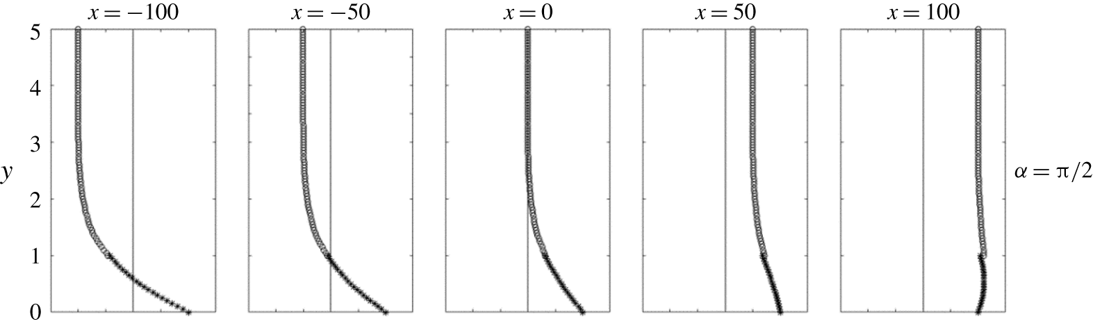
for Rott’s case $\unicode[STIX]{x1D6FC}=\unicode[STIX]{x03C0}/2$ and $U=100$, and the results are shown in figure 1. When they are compared with the results of figure 2 of Rott (Reference Rott1956), it is clear that the two results are in good agreement except that, at large $x$, the present results show a tiny error happening at the junction between the $u(x,y)$ of small and large $y$. This error is due to the approximation taken for both $f(y)$ and $g(y)$, which is then magnified in $f^{\prime }(y)$ and $g^{\prime }(y)$ when (2.8) is calculated. Note please that the horizontal scale $x/(U/\unicode[STIX]{x1D70F})=1$ of Rott’s figure 2 is equivalent to the present case $x=100$, $x/(U/\unicode[STIX]{x1D70F})=-1$ to the case $x=-100$ and $x/(U/\unicode[STIX]{x1D70F})=0$ to the case $x=0$.

Figure 1.

Value of $u(x,y)$ at different positions $x$ for the case $U=100$ and $\unicode[STIX]{x1D6FC}=\unicode[STIX]{x03C0}/2$. The curve denoted by ○ is the solution for large $y$ and the curve denoted by ∗ is the solution for small $y$.

3 The stagnation point position

As discussed by Tamada (Reference Tamada1979), Dorrepaal (Reference Dorrepaal1986) and Tooke & Blyth (Reference Tooke and Blyth2008), the flow structure is closely related to the SP position $x_{s}$ on which the dividing streamline meets the flat plate. According to the definition of SP by Tamada, the shear force vanishes on the SP, i.e. $\unicode[STIX]{x2202}^{2}\unicode[STIX]{x1D713}/\unicode[STIX]{x2202}y^{2}=0$, and the equation for $x_{s}$ is given as

(3.1)$$\begin{eqnarray}x_{s}=-\frac{g^{\prime \prime }(0)}{f^{\prime \prime }(0)}=-\frac{\left(-{\displaystyle \frac{aU}{K}}+G\cos \unicode[STIX]{x1D6FC}\right)}{Ka^{3}}=\frac{0.6585}{\sin \unicode[STIX]{x1D6FC}}U+x_{s0},\end{eqnarray}$$

in which

(3.2)$$\begin{eqnarray}x_{s0}=\frac{-1}{\tan \unicode[STIX]{x1D6FC}}\frac{G}{Ka},\end{eqnarray}$$

where $x_{s0}$ is the SP position for $U=0$ and $G=1.4065$. In deriving (3.1), $f^{\prime \prime }(0)$ and $g^{\prime \prime }(0)$ are obtained by taking double differentiation of (2.4) and (2.6), respectively. It is seen from (3.1) and (3.2) that $x_{s}$ is a function of $U$ and $\unicode[STIX]{x1D6FC}$. 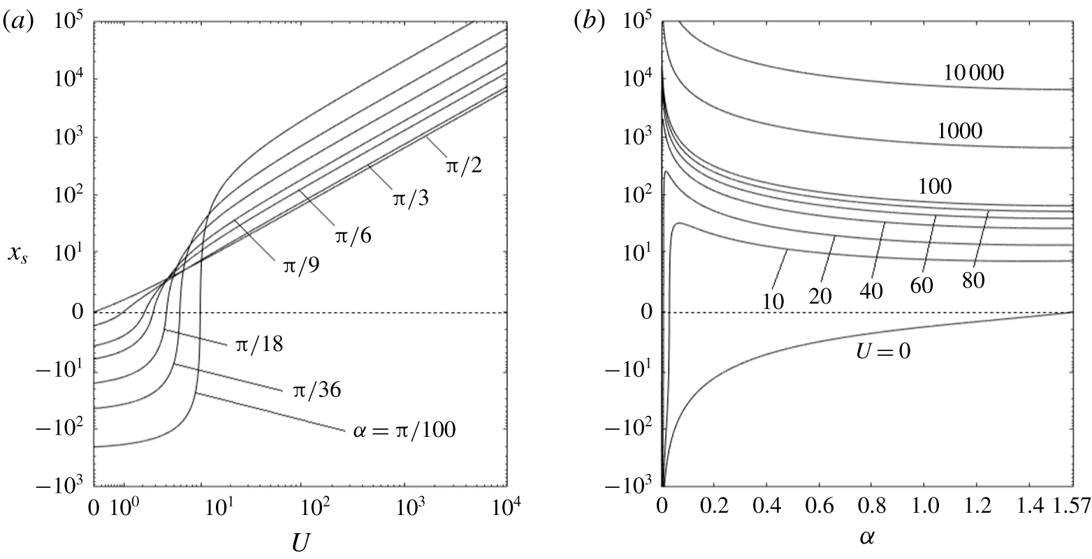To more precisely examine the change of the SP position with these two flow parameters, we calculate $x_{s}$ for a wide range of $U$ and $\unicode[STIX]{x1D6FC}$ and the results are shown in figures 2(a) and 2(b).

Figure 2.

(a) The SP position $x_{s}$ varies with the plate velocity $U$ for different impinging angles $\unicode[STIX]{x1D6FC}$. (b) The SP position $x_{s}$ varies with the impinging angle $\unicode[STIX]{x1D6FC}$ for different plate velocities $U$.

We first examine the effect of plate velocity on the change of SP position, and the results are shown in figure 2(a). By taking the orthogonal SP flow $\unicode[STIX]{x1D6FC}=\unicode[STIX]{x03C0}/2$ as a nominal case, which is the straight line of the figure, it is seen that the SP is located right on the origin of the coordinates (or $x_{s}=0$) when the plate is stationary (or $U=0$). When the plate starts moving ($U>0$), the SP moves immediately downstream ($x_{s}\geqslant 0$). For the non-orthogonal SP flow, say $\unicode[STIX]{x1D6FC}=\unicode[STIX]{x03C0}/3$, the SP stays upstream ($x_{s}<0$) when $U=0$, as predicted by Dorrepaal (Reference Dorrepaal1986) and Tooke & Blyth (Reference Tooke and Blyth2008), while it moves downstream when $U\geqslant 0.932$. Namely, the turning point for the SP moving from upstream to downstream occurs at $U=0.932$. Similarly, for $\unicode[STIX]{x1D6FC}=\unicode[STIX]{x03C0}/6$, the turning point occurs at $U=2.123$, for $\unicode[STIX]{x1D6FC}=\unicode[STIX]{x03C0}/18$ it occurs at $U=4.097$ and for $\unicode[STIX]{x1D6FC}=\unicode[STIX]{x03C0}/100$ it occurs at $U=9.777$. In brief, the results of figure 2(a) suggest that the plate velocity $U$ plays a dominant role in determining the SP position no matter whether the flow is orthogonal or non-orthogonal; the SP moves further downstream when $U$ is larger, which is obviously because the SP moves with the moving boundary due to the no-slip condition.

Now we turn to examining the effect of impinging angle $\unicode[STIX]{x1D6FC}$ on the change of SP position $x_{s}$. As shown in figure 2(b), when the bottom plate is stationary ($U=0$), the SP stays in upstream ($x_{s}\leqslant 0$) for all of the impinging angles considered ($0\leqslant \unicode[STIX]{x1D6FC}\leqslant \unicode[STIX]{x03C0}/2$). According to the curve of $U=0$, the SP stays at the origin when the SP flow is orthogonal ($\unicode[STIX]{x1D6FC}=\unicode[STIX]{x03C0}/2$) and moves to infinite upstream ($x_{s}\rightarrow -\infty$) when $\unicode[STIX]{x1D6FC}\rightarrow 0$. When the plate starts to move with a small velocity, say $U=10$, the SP moves immediately from infinite upstream to downstream when $\unicode[STIX]{x1D6FC}$ is larger than a small critical value ($\unicode[STIX]{x1D6FC}\approx 0.030$). The critical $\unicode[STIX]{x1D6FC}$ becomes smaller when $U$ is larger, for example, $\unicode[STIX]{x1D6FC}\approx 0.008$ when $U=20$, $\unicode[STIX]{x1D6FC}\rightarrow 0$ when $U\geqslant 30$. By and large, for each case of $U\geqslant 10$, the SP moves from upstream to downstream when $\unicode[STIX]{x1D6FC}$ increases from zero to a small critical value. More precisely, the SP first reaches the further-most downstream (a maximum $x_{s}$) and then moves slightly back to upstream gradually (a decreasing $x_{s}$) until it reaches the final position at $\unicode[STIX]{x1D6FC}=\unicode[STIX]{x03C0}/2$.

The results in both figures 2(a) and 2(b) indicate invariably that the SP position is sensitive to the changes of $\unicode[STIX]{x1D6FC}$ and $U$, especially when both parameters are small. Namely, for a great portion of $\unicode[STIX]{x1D6FC}$ and $U$, the SP stays in downstream ($x_{s}>0$); only when $\unicode[STIX]{x1D6FC}$ and $U$ are small can the SP stay upstream ($x_{s}<0$). 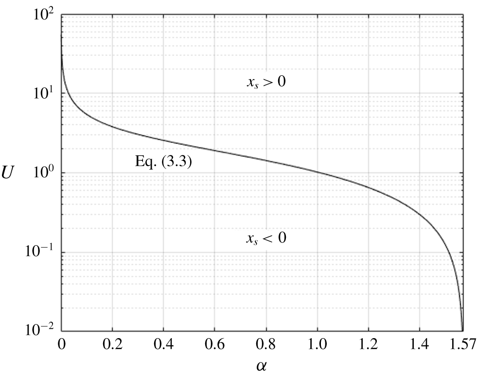To more specifically identify the portion of $\unicode[STIX]{x1D6FC}$ and $U$ at which the SP locates in either upstream or downstream, we calculate the $x_{s}$ of (3.1) in the $\unicode[STIX]{x1D6FC}$–$U$ plane. It turns out that there is a curve $x_{s}(\unicode[STIX]{x1D6FC},U)=0$ separating the $\unicode[STIX]{x1D6FC}$–$U$ plane into two regions: $x_{s}>0$ and $x_{s}<0$. The equation of this curve can be derived from (3.1) and (3.2) when $x_{s}=0$ is considered, yielding

(3.3)$$\begin{eqnarray}U=\frac{1}{0.6585}\frac{G}{K}\frac{\sqrt{\sin \unicode[STIX]{x1D6FC}}}{\tan \unicode[STIX]{x1D6FC}}.\end{eqnarray}$$

We show this curve in figure 3. It is seen that the $U$ for $x_{s}=0$ increases when $\unicode[STIX]{x1D6FC}$ decreases, implying that, for the SP flow with a smaller $\unicode[STIX]{x1D6FC}$, one needs a larger $U$ to keep the SP located on the origin. When $U\geqslant 30$, the SP will is located in the downstream as long as $\unicode[STIX]{x1D6FC}$ is slightly larger than zero. This means that, as soon as the plate moves with a velocity $U\geqslant 30$, the SP will stay downstream as long as the SP flow is not parallel to the plate at the bottom, no matter whether the flow is orthogonal or non-orthogonal.

Figure 3.

The curve of $x_{s}=0$ accounted for by (3.3) in the $\unicode[STIX]{x1D6FC}$–$U$ plane. In the domain of $x_{s}>0$, the SP is located in downstream. In $x_{s}<0$, the SP is located in upstream.

How big is $U=30$ physically? For a fluid such as water, the kinematic viscosity of water at $20\,^{\circ }\text{C}$ is $\unicode[STIX]{x1D710}\cong 1\times 10^{-6}~\text{m}^{2}~\text{s}^{-1}$. Since the distance is non-dimensionalized by $\sqrt{\unicode[STIX]{x1D710}/\unicode[STIX]{x1D70F}}$ and the velocity by $\sqrt{\unicode[STIX]{x1D710}\unicode[STIX]{x1D70F}}$, $U=1000$ means the dimensional velocity is approximately $1~\text{m}~\text{s}^{-1}$, and $x_{s}=1000$ is approximately 1 m. For a fluid such as liquid metal, the kinematic viscosity $\unicode[STIX]{x1D710}\cong 0.617\times 10^{-6}~\text{m}^{2}~\text{s}^{-1}$ at $2000\,^{\circ }\text{C}$, $U=1000$ is equivalent to a dimensional velocity of $0.785~\text{m}~\text{s}^{-1}$, $x_{s}=1000$ to a distance of 0.785 m. Based on these scales, $U=30$ is approximately $0.030~\text{m}~\text{s}^{-1}$ for water and $0.024~\text{m}~\text{s}^{-1}$ for liquid metal, which is indeed a minimal value in reality.

Although the present study considers neither the heat transfer through the moving plate nor the solidification of the liquid metal, the results may still shed light on the flow occurring in the fast solidification of non-crystal steel film. In the fast-solidification process, in general, the impinging angle is $\unicode[STIX]{x1D6FC}\sim \unicode[STIX]{x03C0}/2$ and the plate velocity is approximately $25~\text{m}~\text{s}^{-1}$ (Steen & Karcher Reference Steen and Karcher1997), which is equivalent to the case $U\sim 32\,000$ corresponding to $x_{s}\sim 21\,000$, being equivalent to a distance of approximately 16.4 m downstream of the origin. That means that, as the liquid metal impinges vertically on the fast-moving plate, the SP will move downstream to a considerable distance compared with the gap width of the nozzle, which is usually of the scale of a millimetre. This result suggests that the flow of liquid metal above the moving plate essentially divides into two parts by the dividing streamline. The flow below the dividing streamline confines in a shallow boundary layer, which is nearly parallel to the flat plate for a long distance. Since the boundary layer thickness is closely related to the SP position, a designated heat transfer rate to solidify the liquid metal may be achieved by choosing a proper $U$ and $\unicode[STIX]{x1D6FC}$. Consequently, equation (3.1) may become a practical scheme to indicate an appropriate direction for the improvement of the quality of the fast-solidification process.