

Farming in arid and semiarid regions is largely a story about managing limited water. In the Americas, according to ethnographers, post contact era farmers of the greater Southwest used a sophisticated and diverse array of water management strategies suited to their environments, as did their farming ancestors. Some approaches to the study of Southwest farming have focused on the ability to grow maize and its productivity in a particular area given environmental factors (Benson Reference Benson2010; Benson et al. Reference Benson, Ramsey, Stahle and Petersen2013; Kohler et al Reference Kohler, Bocinsky, Cockburn, Crabtree, Varien, Kolm, Smith, Ortman and Kobti2012). Others have looked at variability in farming techniques archaeologically, ethnographically, or experimentally (see Supplemental Text 1). We investigate expected variation in a simple irrigation strategy using an optimization model with empirical data collected from maize farming experiments. The goal is to demonstrate that formal models for exploring the trade-offs between the costs and benefits of irrigation can focus and strengthen experimental, archaeological, and ethnographic research, allowing increasingly rigorous predictions about which water management strategies provide an adaptive advantage and under what circumstances.
This work contributes to understanding the variation in Southwest farming strategies in several ways. First, we focus on the day-to-day decisions of farmers working optimally to increase farming efficiencies where efficiency is measured by return rate. These decisions are made under specific environmental constraints with the expectation that the time and effort invested in each farming activity will influence the resulting yield. The value of investment in any activity is balanced with the benefit lost from not investing that time or energy in another activity. This is the opportunity cost. We show that the investment in and implementation of various farming strategies falls along a continuum of success or failure in terms of crop production, with the interesting cases falling somewhere between the extremes. Our approach sets up experimental methods and uses a simple optimization model for investigating farming activities with varying opportunity costs and environmental contexts that determine where productivity falls along that continuum as investments change.
Second, understanding the relationship between a farming strategy and its efficiency in a particular environmental context requires data collection on the costs and benefits. These are best measured in actualistic farming experiments. Examining just the costs without knowing the benefit or just the benefits without knowing the costs would lead to inaccurate generalizations. Similarly, comparisons of costs from one ethnographic or environmental context and the benefits from another is always suspect because the costs and benefits are often correlated in environmentally specific ways. Actualistic experiments allow the collection of empirical data by systematically varying the costs to study the underlying processes related to benefits. The ethnographic literature contains little data on the payoff for varying the intensity or frequency of farming activities. Ethnographic discussions of labor investments in farming are often anecdotal, or the source or method of collection of empirical data is unclear. We present a case study for collecting cost and benefit data for simple diversion irrigation in a well-documented environmental context. This research provides baseline estimates and an experimental protocol that other researchers interested in the spread of agriculture in arid lands should find useful. These represent minimum estimates in the efficiency of various farming activities because we are low on a steep learning curve, but repeated experiments have incrementally improved our understanding of maize farming, irrigating, and the broader implications of making decisions in a challenging environment.
Last, we provide an example of conducting systematic research in the present based on a general theory of behavior to inform on when irrigation farming would have been an adaptive strategy in the past. Our model sets rate maximization as the goal based on the general premise that efficiency in subsistence activities is strongly favored by natural selection (Davies et al. Reference Davies, Krebs and West2012; Stephen and Krebs Reference Stephens and Krebs1986). As is true for all formal models from behavioral ecology, the optimal irrigation model (OIM) is a simplification of the complex and interrelated trade-offs related to farming. The simplification provides theoretical support for some long-standing generalizations about irrigation while challenging the veracity of others.
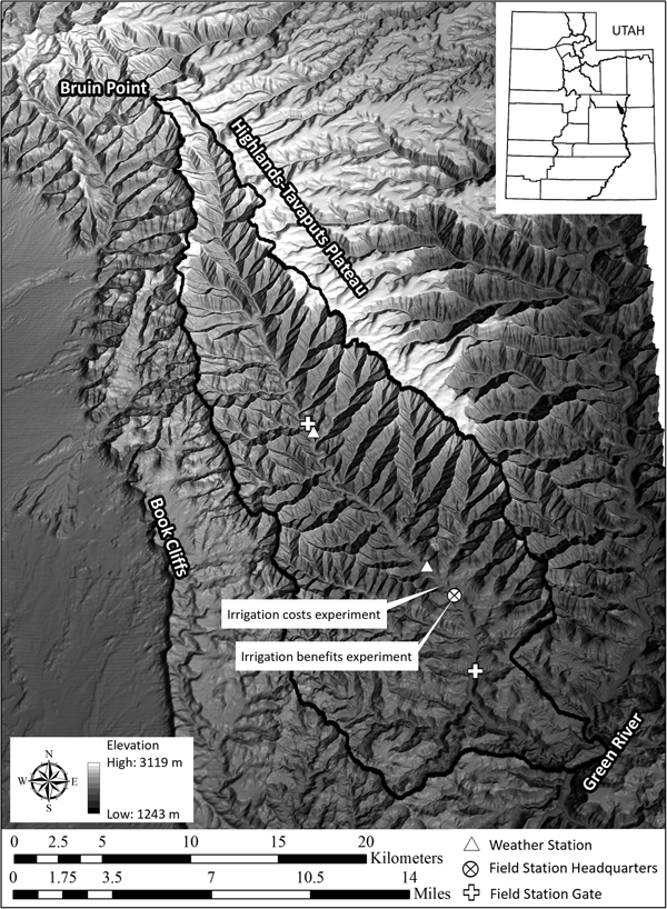
The stimulus for this study is to better understand the opportunities and constraints faced by prehistoric farmers in Range Creek Canyon (Figure 1) and how they influence prehistoric settlement patterns (Boomgarden Reference Boomgarden2015). We focus on simple diversion irrigation from Range Creek, an obvious source of irrigation water in this canyon that was intensively occupied by Fremont farmers from around AD 900 to 1200. Following the foundation established by Barlow (Reference Barlow2002), irrigation is modeled as one of many activities related to farming, such as clearing fields, planting, fertilizing, weeding, and harvesting—all activities that exact a cost with an expectation of an increase in crop yield. Although focused on the research in Range Creek Canyon, the perspective provided by the model and the reported data have general implications about the challenges of farming, past and present, in dry environments worldwide.
Relief map of area around Range Creek Canyon located on the West Tavaputs Plateau, east-central Utah. Note the location of two weather stations, the field station headquarters, and two maize farming experiments. Map by Duncan Metcalfe and Shannon Boomgarden.

When and How Much to Irrigate
Foraging theory suggests that the decision whether to farm is dependent on the expected return rate for farming and that of its alternatives, in this case hunting and gathering wild resources. If the expected return rate for farming is higher than that expected for hunting and gathering in a particular environmental and social context, then farming is predicted. Embedded in the expectation of the return rate for farming are estimates about how time spent in individual farming activities will influence the yield. It may be worth spending two days weeding a field but not three, depending on the relationship between the amount of time spent weeding and the crop yield. The interesting parts of these generally continuous functions are when their slopes are greater than or equal to zero.
Irrigation is a case in point. The extremes are obvious. When farming occurs where it is impossible to produce a crop without irrigation, it is reasonable to infer farmers practiced some form of irrigation. Conversely, when documenting past farming activities where there is no benefit to irrigating farm fields, archaeologists infer that irrigation was not practiced. The interesting cases are found where irrigation is not necessary to grow a crop, but the yield can be improved with irrigation. In these areas, the question is whether and how much farmers should irrigate. The answer depends on the labor costs, benefits in yield, and opportunity for doing so.
A variety of irrigation techniques are ethnographically documented in the Southwest. Each has strengths and weakness that can only be evaluated in the context of the setting. Important considerations in deciding which irrigation technique or set of techniques to employ will include 1) the presence and character of available surface water; 2) the costs of constructing and maintaining features required to slow, capture, retain, or divert the flow of water; and 3) the relationship between the time invested in constructing each feature and their use-life and efficiency in delivering water measured in increases in expected grain yield.
In this paper, we assume the farmers have chosen to farm given their expectations concerning each variable, including whether to irrigate. The OIM is designed to predict the intensity of irrigation when the chosen irrigation technique provides the farmer some control over the timing and length of irrigation events. The OIM does not directly inform the researcher whether a potential farmer in a particular place or time should farm; it simply predicts the costs and benefits of irrigating within the larger matrix of individual decisions and expectations that combine to construct that broader decision.
Background and Fundamentals of Irrigation
In dry regions, available soil moisture is a critical constraint on successful farming. Although transpiration accounts for about 99% of the water used (Gardner et al. Reference Gardner, Pearce and Mitchell1985:23), moisture is critical for a number of physiological processes related to growth, development, and reproduction. The moisture available in the soil is a function of soil texture, structure, and organic content (Rhoads and Yonts Reference Rhoads and Yonts1991; Shaw Reference Shaw, Sprague and Dudley1988). The soil within the root zone of the plant is where the moisture available to crops is stored between inputs of additional water. Between these events, water is more or less continuously lost (although not at a constant rate) through evaporation and transpiration. These two processes are generally measured as a single phenomenon labeled evapotranspiration (Shaw Reference Shaw, Sprague and Dudley1988).
In the simplest case, the net input of moisture relative to the loss of moisture through evapotranspiration determines the water budget of the field. Ideally, the soil moisture is replaced before half the available water in the root zone is lost to evapotranspiration. On days with high ambient temperature and low humidity, wilting will occur during the daytime when half the available soil moisture is depleted. When depleted further, greater effort is required to absorb the needed moisture, and the physiological consequences of water stress, including reduced grain yield, become increasingly serious.
Many Southwestern archaeologists cite Shaw (Reference Shaw, Sprague and Dudley1988:611) for a lower limit of 15 cm of rainfall during the growing season for maize farming. Less attention is paid to his comment that additional moisture will produce larger harvests. The generalization that 15 cm of rainfall is required to grow maize has little meaning without specifying the moisture available in the soil at the time of planting; the water-holding capacity of the soil; the frequency, duration and intensity of the rain events that contribute to that 15 cm; and the productivity of a particular maize variety under these circumstances. Maize might grow with 15 cm of rainfall during the growing season, but the yields are likely to be disappointing relative to what could have been realized with greater moisture. From an economic standpoint, the decision whether to provide supplemental water to what is naturally available should be a function of the cost of that supplemental water relative to the benefit of a larger harvest.
The relationship between the amount of water received by a crop and the harvest yield is often referred to as the water–crop production function or water production function (Supplemental Text 2). It has long been recognized that moisture stress during the reproductive stage of maize development is significantly more detrimental to crop yield than the same intensity and duration of stress occurring during the early vegetative stages. Shaw (Reference Shaw, Sprague and Dudley1988:Table 10-1) summarizes earlier studies and estimates that yield reductions are in the order of 2%–13% per day of serious moisture stress when the plant is producing tassels and silk, 4%–7% per day when the ear is filling, and only 2%–4% per day during the late vegetative stage. Another difficulty in modeling crop-production functions is that the effect of each irrigation on harvest yields is partly dependent on all other irrigations (Supplemental Text 2).
The maximum crop yield is achieved when the amount of water lost through evapotranspiration is replaced in a timely manner. Under these circumstances, maize will not suffer moisture stress. The generalized relationship between stages of growth and development and water requirements are shown in Supplemental Figure 1 (based on a long-term study of hybrid maize grown in Nebraska; Kranz et al. Reference Kranz, Irmak, van Donk, Yonts and Martin2008:Figure 1, Table I). The y-axis is scaled to the proportion of the maximum daily moisture needed to avoid stress. The actual maximum value is likely to be a function of maize variety, local weather, and plant spacing, but the sequence of proportional water demands provides a proxy for anticipating the relationship between maize growth and development and the severity of the consequences of moisture stress. Ethnographic data show farmers in the Southwest have adapted a variety of techniques to replace water lost through evapotranspiration and minimize the effects of water stress.
We define farming techniques in two broad categories: those that rely on available water and those that rely on providing supplemental water from either permanent or intermittent sources (Supplemental Text 1). Rainfed (dry farming), water-table, seepage, and flood-farming (runoff) techniques all rely on placing fields in specific locations to take advantage of available water with little to no additional investment in water management.
Techniques that provide supplemental water include those strategies that require the construction and management of surface features to move, direct, or otherwise control intermittent or permanent surface water. The level of investment in irrigation features range from minimal to large, as demonstrated in numerous ethnographic accounts (Supplemental Text 1). Unfortunately, those accounts do not offer reliable quantitative data on the return rates of varying farming techniques (especially those relying on only simple tools). Therefore, gathering empirical data on the costs and benefits of using farming techniques that include investment in irrigation is the focus of our experiments.
Optimal Irrigation Model
Agronomy research is increasingly focused on the costs of irrigation as well as its associated benefits. With expanding regional populations, warming climates, and increasing competition for water, the cost of irrigation has risen substantially. A number of studies have demonstrated that the optimal amount of supplemental water, considering the cost of irrigation, is less than the amount required to produce maximum crop yield per unit area (Supplemental Text 2). This research is often framed as the investigation of deficit irrigation but more recently as optimal irrigation (English et al. Reference English, Solomon and Hoffman2002; see also Supplemental Text 2). Some of the best general discussions of this topic are by Marshall English and his colleagues (English and Raja Reference English and Raja1996; English et al. Reference English, Solomon and Hoffman2002). The following discussion closely follows those works.
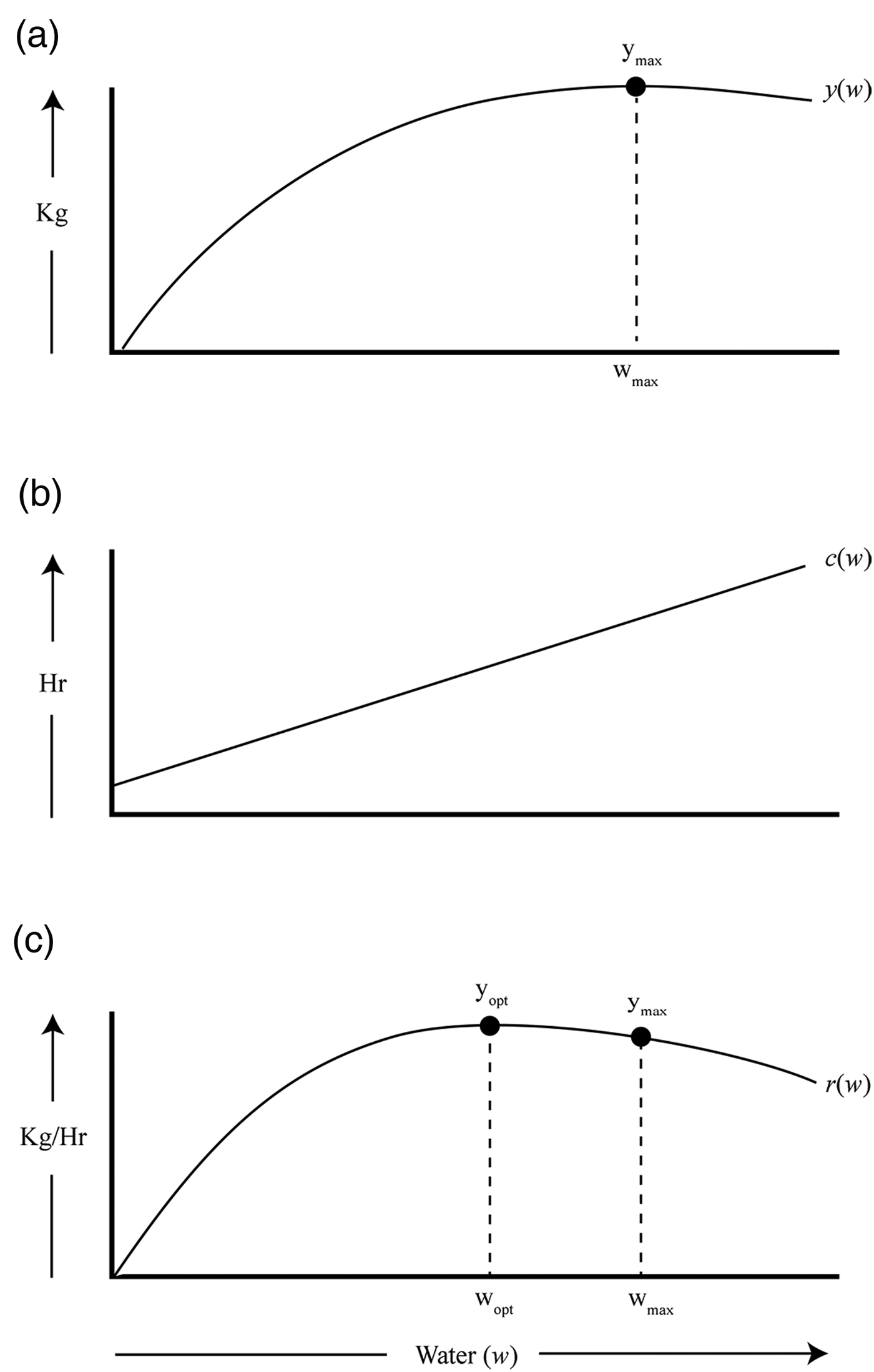
Figure 2a illustrates the idealized relationship between water (w) and crop yield as a function of the amount of available water (y(w)). The maximum crop yield is y max , and w max is the corresponding amount of water required to achieve that yield. W max is equivalent to the maximum total evapotranspiration of the crop during the growing season. Additional water above and beyond w max is wasted since it does not improve crop yield. A reasonable scale of benefit for quantifying y(w) is a measure of the variation in grain yield per unit area as a function of available moisture.
Conceptual model of the ideal relationship between crop yield (y(w)), cost of irrigation (c(w)), and return rate (r(w)). (a) graphically represents the crop water production function, the relationship between water and harvest yield. (b) graphically represents the cost of adding irrigation water to the field. (c) represents the return rate for irrigating.

Understanding the benefits of behavioral options is typically only half the story and often not the more interesting half. Figure 2b illustrates a linear cost function where the y-intercept is the capital costs of irrigation, and the slope reflects the operating costs. For surface irrigation, the capital costs are building the irrigation system. The ongoing costs are those for maintaining and operating that system. Costs are measured in hours of labor per unit area irrigated.
When estimates of the benefits (y(w)) and costs (c(w)) are available, the decision of how much water to add through irrigation can be explored using optimality modeling with the goal of maximizing rates of return. Return rates (r(w)) are simply the benefits divided by the costs. The rate of return for irrigation is:
 $$r\lpar w \rpar = \displaystyle{{y\lpar w \rpar } \over {c\lpar w \rpar }}$$
Figure 2c illustrates the result of performing this operation on benefit and cost functions similar to those in Figure 2a and 2b. Here the rate of return reaches a maximum and then declines with additional water because the benefit accrued from the additional water is outweighed by the additional cost. The water associated with the maximum return rate is the optimal amount of irrigation water (w opt). Less or more water than w opt produces lower rates of return. When y(w)and c(w) are modeled algebraically, then r(w)max is calculated as the positive rate when the first derivative of r(w) is equal to zero. This model is only appropriate when there is some cost associated with irrigation, otherwise r(w) is undefined. Equally important, supplemental water that is cost-free should not be classified as irrigation.
The benefit function (y(w)) is the product of the physiological and environmental demands on the maize crop and their expression in variation in grain yield. Various farming activities can certainly influence the size of the harvest (choice of maize variety, weeding, fertilizing, etc.), but the basic form of y(w) should be roughly constant for a particular maize variety in a specific environmental setting. The cost function, however, is entirely the result of the decisions made by the farmer. For instance, the y-intercept of the function is the effort required to build the infrastructure of the irrigation system; the slope of the function is the effort required to maintain and operate it. These two costs are likely to be related in interesting ways. A well-built dam might have a fairly high capital cost but might reduce the operating cost of the entire irrigation system relative to a less well-built dam. The cost of irrigation for any w i, however, is the sum of both the capital and operating costs, and one is not more important than the other when calculating the return rate for w i. That is, when determining the return rate contribution of irrigation to the broader goal of farming efficiency, both operating and capital costs are important.
The OIM provides several important insights. First, it reinforces the concept that the relationship between water and crop yield is a continuous function that under many circumstances is reasonably approximated by a diminishing return curve. While total failures of a crop and total success certainly occurred, the vast majority of crop yields likely fell between these two extremes. Second, when the costs of irrigation are greater than zero, the optimal yield will be less than the maximum yield per unit area. It is the operating cost that determines the distance between the optimal yield and the maximum yield. The steeper the slope of the cost function, the smaller the optimal yield will be relative to the maximum yield. Last, the model specifies the broad set of circumstances when irrigation is not an economically viable strategy—those circumstances when the ratio of benefits to costs is less than those of alternative strategies.
The OIM is sufficiently robust to provide insights into the costs and benefits of many forms of irrigation. It does not, by itself, predict whether farming is expected in a particular locale. Irrigation is only one of a number of activities that combine to determine the return rate for farming. Others, such as preparing the field, planting, weeding, fertilizing, managing pests, harvesting, and processing for consumption, contribute to the return rate for farming. Fortunately, at least several of these should take the form of a diminishing returns function when harvest yield is plotted against time spent in the activity. Many of the costs and benefits of these farming activities likely interact with one another, and understanding those interactions will require careful investigation.
There is no set threshold for when farming is expected; that decision is a function of the return rates of alternative subsistence strategies relative to that for farming (Barlow Reference Barlow2002). In locales where the return rate from hunting and gathering wild foods is low, the return rate for farming can also be relatively low but still the better choice as long as it produces return rates higher than those for foraging. When the return rates for hunting and gathering are relatively high, farming is only expected when its return rates are relatively high but slightly better than the alternatives. Farming is a complex process with many components. Breaking farming into its constituent pieces and investigating each is the first step to understanding the trade-offs inherent in this subsistence strategy.
Range Creek Canyon Maize Farming Experiments
Two sets of maize farming experiments using simple diversion irrigation from a perennial creek were conducted in Range Creek Canyon between 2013 and 2017 (Figure 1). The first set, conducted over a five-year period, was designed to investigate the relationship between edible grain yields and the amount of supplemental water supplied to multiple maize plots (Boomgarden Reference Boomgarden2015). These experiments determined the water–crop production function (benefits for irrigation). The second set of experiments, conducted over a three-year period, was designed to investigate the costs of constructing and operating a basic diversion irrigation system using only simple tools (Simons Reference Simons2017). These experiments determined the linear cost function where the y-intercept is the up-front or capital costs of irrigation and the slope reflects the ongoing or operating costs. The cost and benefit experiments were conducted separately because they were designed to produce very different types of data. Together they produced the complementary data required to use the OIM to examine the return rate for irrigation in Range Creek Canyon.
Water–Crop Production Experiment
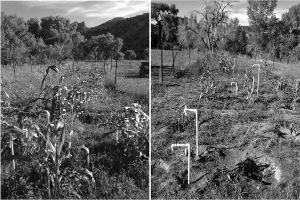
The water–crop production experiments were located at the field station headquarters (FSH) in a relatively flat area with access to an existing surface diversion irrigation system (Figure 3). Tohono O'odham 60-day maize (Zea mays) was planted in multiple plots measuring an average of 28 m2. This variety was chosen for its adaptation to arid environments, specifically its short growing cycle (Muenchrath Reference Muenchrath1995). Maize was planted in basins spaced 1 m apart, following ethnographic accounts (Supplemental Text 1). Twelve basins with five seeds each were planted in each plot, all irrigated at the time of planting to ensure germination. Plots were weeded as needed.
(Left) Overview photograph of the water-crop production experiment located at the Field Station Headquarters in Range Creek Canyon. Photograph was taken facing north with Plot 6 (irrigated every day) in foreground. (Right) Overview of the maize plots, taken facing south with Plot 1 (not irrigated) in the foreground. PVC pipes indicate the location of soil moisture sensors. Both photographs were taken August 5, 2015 (photographs by Shannon Boomgarden).

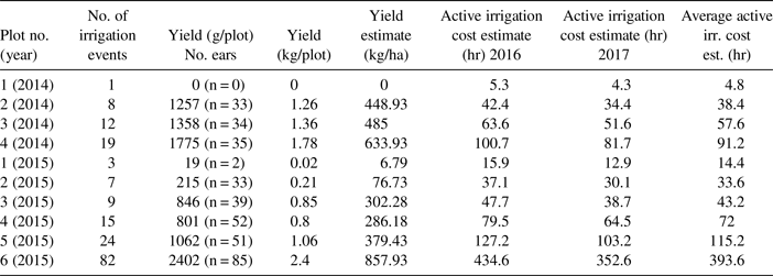
The number of irrigation events for each plot is shown in Table 1. Plots were irrigated for a standard length of time for each application. To document the timing of growth stages and water stress, we periodically photographed the basins and described the plants (Supplemental Figure 2). Soil moisture was monitored directly and indirectly. A manual rain gauge located at the FSH recorded the amount of rain. These data augment the data from two automated weather stations (Figure 1).
Summary of Crop-water Production Experiments.

Only 2014 and 2015 produced reliable data on the relationship between soil moisture and crop yield. Pest damage during the other three years was sufficiently severe to compromise the results. Even then, corrections were required to accommodate pest damage for the 2014 (see Boomgarden Reference Boomgarden2015:46–47) and 2015 data. In 2015, raccoons damaged the experimental gardens shortly before the harvest, eating kernels from multiple ears. The damaged ears and ear fragments from each plot were collected, and a minimum number of damaged ears per plot was estimated. Based on the average kernel weight per undamaged ear for each plot, the weight of the missing kernels was estimated.
The benefits to watering were calculated by weighing the dried edible kernels from each maize ear and summing the total grain yield from each plot. Edible grain weight was compared across plots to show variability related to the amount of irrigation water. The totals for each 28 m2 plot were scaled up to estimate the yield in kilograms per hectare and plotted by the number of watering units. The amount of water added during irrigation would be the best measure for determining the water-crop production function. Unfortunately, this was not possible, so instead the water flow was held constant and was timed.
Table 1 summarizes the yield for each season of the water–crop production experiment. While it is reasonable to simply multiply the harvest yield per plot by the number of plots in one hectare (357.14), this is not true for irrigation time. Each irrigation event lasted 20 minutes for each experimental plot; the goal was to ensure that individual plots were soaked with the same amount of water. However, simply multiplying the number of plots in a one-hectare field by 20 minutes produces a very large number because it does not account for the economy of scale in irrigation. By examining a subset of our cost experiments, we found that one hectare required 45 hours of irrigation time to evenly saturate ~12 inches below the ground. Allowing irrigation water to saturate the field 45 hours per hectare is not the same as the time spent in active irrigation. The time required to irrigate 0.25 acres averaged about 25 minutes: 5 minutes to set the dam to divert water from the main ditch and another 20 minutes to clear furrows of obstructions. Based on this estimate, 1 ha would require about 4.2 hours of active irrigation (irrigation costs) to allow water to run on the field for 45 hours (not including main dam maintenance). These calculations are the source of the time estimates in Table 1.
The size of a field that can be irrigated per event is a function of the volume of water available for diversion, the slope of the field, the soil infiltration rate, and the existing soil moisture. These are all context specific. To generalize the results of our experiments (and because we do not have a direct measure of the volume of water (w) added to the field per event), we define w u as the water added to a field per irrigation event, y(w u) is the benefit of adding that water, and c(w u) is the cost.
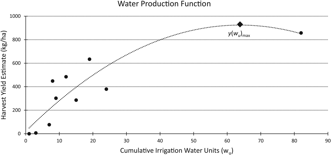
Figure 4 shows the result of fitting a second-order polynomial regression to the yield and time data per hectare. While these results are based on a small sample and the data point at 82 w u (858 kg/ha) has a large influence on the regression, other studies suggest that the relationship should be well described by a quadratic function (English and Raja Reference English and Raja1996). The regression is as follows:
 $$\eqalign{y\lpar {w_u} \rpar & = \; -0.2219w_u^2 \; + \; 28.317w_u\; \cr & \quad + \; 20.69}$$
Across the five years of experiments, the plants in the plots that were not irrigated after germination produced no mature ears. In irrigated plots where the soil moisture was not fully replenished, the plants experienced significant stress, especially during the reproductive phase. Despite not having yield totals for all years, it was evident throughout the experiments that flooding the field at least twice per week significantly improved the production of maize.
Data points from 2014 to 2015 maize farming experiment yield showing water–crop production function y(w), the results of fitting a second order polynomial regression to the data  $(y\lpar {w_u} \rpar = -0.2219w_u^2 + 28.31w_u + 20.69; \; r^2 = 0.75)$.

Costs Experiment
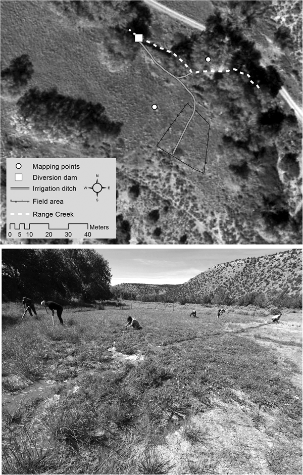
From 2015 to 2017, we quantified the cost of simple surface irrigation by constructing and maintaining diversion dams and ditches and irrigating an experimental field of maize. Costs were recorded on agricultural activities, such as time spent clearing the field and planting the maize, to provide a better basis for comparison with other experimental and ethnographic examples. Only simple tools were used in these activities. The location of the “cost” experimental field was chosen because it was relatively level and within a short distance of a section of creek that was not deeply entrenched (Figure 5). To restrict pests, a roughly 530 m2 area was fenced for the maize garden. Sediment, consisting of sandy loam and gravels, was removed from ditches with digging sticks and bark scoops. In 2015, 55 m of ditch were dug. In 2016, 13 m were dug, and in 2017, 69 m were dug. The average ditch width ranged from 26 cm to 30 cm and ranged in depth from 14 cm to 25 cm. The entire creek had to be dammed to raise the water level sufficiently for it to run into the main ditch.
(Above) Overview map of the irrigation cost experiment location. (Below) Field being irrigated by students using simple tools (photograph by Shannon Boomgarden).

Participants in the experiments included female and male students and staff ranging in age from 18 to 50 years. Participants began with no experience; in subsequent years, the staff instructed students on the most efficient techniques discovered in previous years. While our results provide only a minimum estimate of what the Fremont return rates might have been, given their greater knowledge of farming techniques, we were easily able to get water to fields and became more efficient each year.
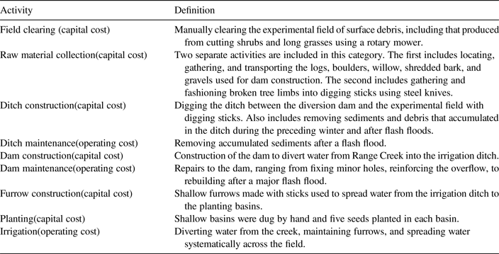
Work activities are divided into seven categories (Table 2). Each participant recorded the amount of time spent on each activity. Constructing an irrigation system involves bouts of strenuous work, and rest breaks were enforced and included in activity times. The goal was not to see how fast each of these activities could be completed but to determine how much time they required if the effort had to be maintained over several days or weeks. Using insights gained from the OIM, we classified time spent in each activity as either a capital construction or operating cost.
Definitions for Work Activities.

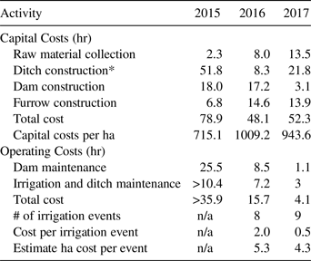
At the end of each season, times were summed for each activity. Some activities were then scaled to represent costs in terms of person-hours per hectare (Table 3). A series of assumptions are made to calculate per-hectare cost estimates. The times required for clearing and planting the field are assumed proportional to field size, so the experimental results are multiplied by 81.3 (2015) and 62.5 (2016 and 2017) to scale the results up to one hectare. We assume that one dam could divert sufficient water to irrigate one hectare of land, so dam construction costs are not scaled. Time spent digging ditches is scaled with the assumption that a square one-hectare field requires a 100 m long header ditch. The cost of digging the header ditch was estimated based on digging rates recorded during the experiments (Table 3). This estimate was added to the actual costs of the ditches connecting the creek to the field.
The difficulties of scaling time spent irrigating to a one-hectare standard presented even more of a challenge because we tried to measure the time required to irrigate. The problem is that irrigation naturally intertwines with other field activities. Once the water is diverted into a particular section of the field, students spent their time not only monitoring the water flow but also pulling weeds, killing pests, and clearing the field. The notes are often insufficiently detailed to distinguish the times spent on different field activities, and the differences are glossed over as “irrigation.” The second problem is that the irrigation crews frequently consisted of several people, so time spent irrigating is multiplied by the number of crew members even for those times when only one person was actively involved in irrigation. As a consequence, the values presented in Table 3 for “total cost” are unrealistically high. For these reasons, 4.2 hr/ha is used as the episodic cost of irrigating one hectare with the costs of dam maintenance, which is an easily segregated activity, added to that value.
Summary of Irrigation Costs by Activity.

* Rate for ditch digging (m/hr) increased each year 1.06 (2015), 1.58 (2016), and 3.17 (2017)
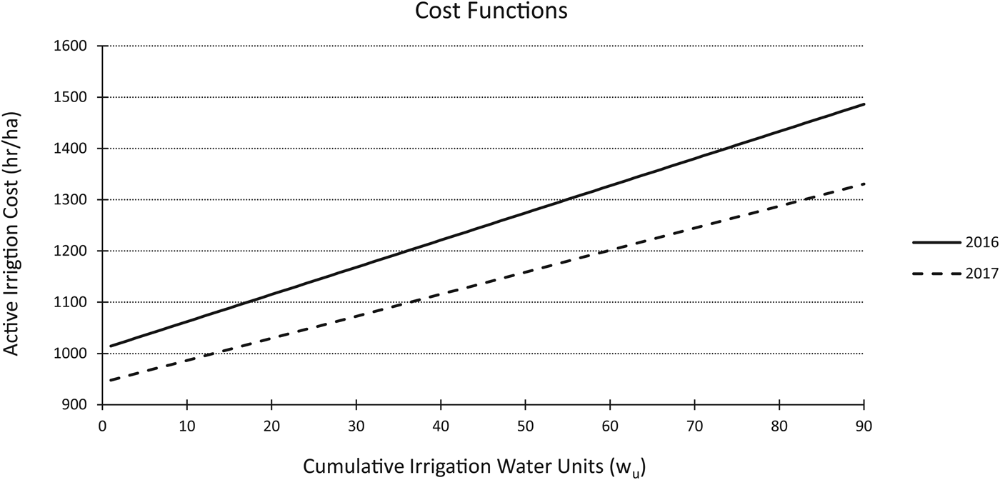
The cost function is modeled as a linear function where the capital investment is the y-intercept and the operating costs per irrigation event determine the slope (Figure 6). Operating costs are divided by the total number of irrigation events per season to estimate the average time spent on each event (Table 3). It would be best to have a measure of the number of hours required per unit-volume of water applied to the experimental field, but for the reasons described earlier, time spent on individual irrigation events is the best proxy available for the costs of irrigation. The OIM is designed to measure the costs and benefits of irrigation, so only activities related to the water-management strategy are incorporated. Operating costs include maintaining the dams and ditches and spreading water across the field using digging sticks. Due to some missing data from the 2015 pilot study, c(w u)was only calculated for 2016 and 2017. This yields the following cost equations:
 $$c\lpar {w_u} \rpar _{2016} = 5.3w_u + 1009.2$$
 $$c\lpar {w_u} \rpar _{2017} = 4.3w_u + 943.6$$
Total time spent by activity and by year are listed in Table 3. We anticipated that costs for capital activities would decrease across years mainly as a function of some features being reused and partially as a function of the staff becoming familiar with the skills required to efficiently complete each task. In some cases, these expectations were met. Ditch construction was very time-consuming in 2015, when the feeder ditch from the diversion dam to the field was first constructed. In subsequent years, the ditch only had to be de-silted, although a heavy spring stream flow in 2017 made this a more time-consuming task than in 2016. The time spent in raw material collection increased from one year to the next. This is a function of having to spend more time each year in search and transport of suitable materials.
Chart showing the cost function c(w) for both 2016 and 2017, modeled as linear functions. Capital investment determines the y-intercept and operating costs per irrigation event determine the slope.

The most interesting part of the experiment was observing the participants as they worked together to learn efficient building strategies. When participants were allowed to collaborate, the rate of ditch construction nearly doubled. The speed of ditch construction improved across all three years despite the inexperience of student participants.
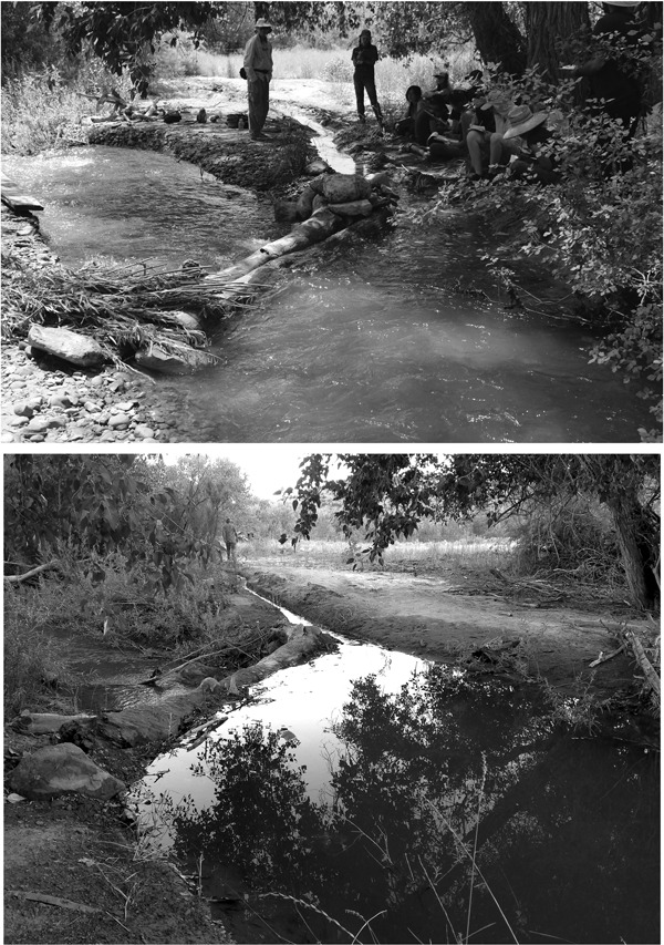
Another example of learning relates to the first dam built. A large (3.6 m long, 0.7 m diameter) dead tree wedged between the two walls of the creek channel provided the base of the first dam, requiring great effort to transport and position. This costly dam raised the level of the creek a full meter and was expected to require only minor maintenance in subsequent years. Unfortunately, a moderate flash flood 15 days later destroyed the dam, and it had to be rebuilt. Subsequent dams were also destroyed by flooding, but over the first two years, the base of the channel was raised more than a half meter due to gravels and sands collecting behind earlier dams (Figure 7). By 2017, we learned that the minimum investment necessary to divert the water into the ditches was the best strategy for reducing the costs of rebuilding dams after flash floods (Figure 7).
Photographs from the irrigation costs experiment showing the second dam constructed in 2015 (above) and the dam constructed in 2017 (below). The shape of the creek bank changed significantly between years. By building a less substantial dam in 2017 compared to 2015, the investment was lowered and the efficiency increased (photographs by Shannon Boomgarden).

OIM Results
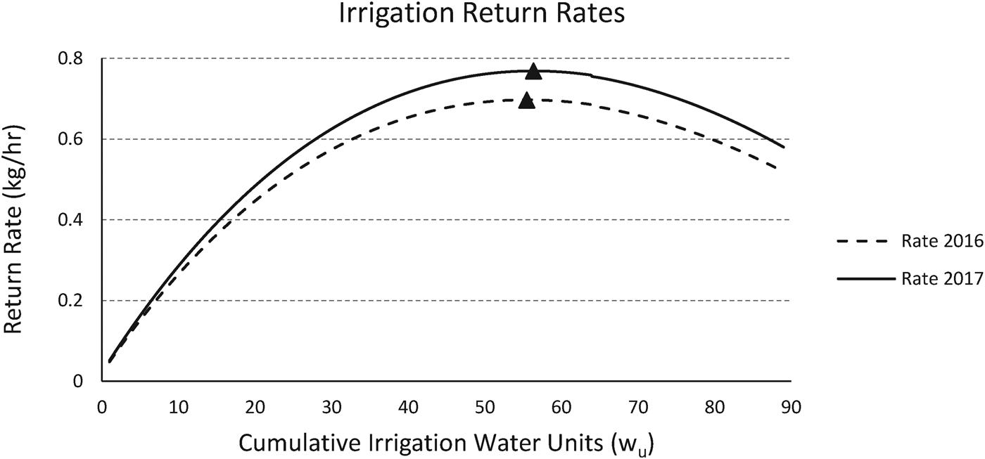
When just the benefits are considered, the obvious solution is to apply as much supplemental water as needed (y max) to obtain the maximum yield. Additional water is wasted effort. When costs are combined with benefits, the optimal solution is to maximize the rate of return (r(w u); Equation 1). The experimental data provide two estimates of that rate of return, one for 2016 (Equation 3) and 2017 (Equation 4):
 $$r\lpar {w_u} \rpar _{2016} = \displaystyle{{-0.2219w_u^2 \; + \; 28.317w_u\; + \; 20.69} \over {5.3w_u + 1009.2}}$$
 $$r\lpar {w_u} \rpar _{2017} = \displaystyle{{-0.2219w_u^2 \; + \; 28.317w_u\; + \; 20.69} \over {4.3w_u + 943.6}}$$
For 2016, the maximum rate yields 0.70 kg/hr for Equation 5 (Figure 8a) and 0.77 kg/hr for Equation 6 (Figure 8b). As expected, y(w u)opt is less than y(w u)max in both cases (for 2016, 907 kg/hr versus 922 kg/hr; for 2017, 910 kg/hr versus 922 kg/hr). Because the slope of the cost function for 2016 is greater than that for 2017, the difference between y(w u)max and y(w u)opt is greater for 2016 than for 2017.
Return rates as a function of time spent irrigating for cost functions from 2016 and 2017. Triangles indicate the optimal return rates.

It is worth reviewing selected assumptions that underlie the calculated estimates for y opt because several uncertainties are introduced by using measures of time as indirect measures of both the benefits and costs of irrigation rather than benefits (kcals) and costs (hr) per unit volume of irrigation water. First, the volume of water per unit time, the rate at which water is added to the fields, is assumed to be consistent between irrigation events. Second, the rate of irrigation water applied to any field is assumed to have been the same across irrigation events. Last, ensuring that all portions of a field receive a uniform amount of water requires attention and effort on the part of the farmer. Like many farming activities, that effort and its consequences likely diminish returns. In all the cases above, we attempted to maintain consistency from one irrigation event to the next and between experimental fields. Nevertheless, it would be useful to implement an objective scale to ensure consistency.
For purposes of modeling, capital and operating costs were defined as mutually exclusive and independent. In reality, time spent in capital investment may change operating costs. For example, spending more time constructing a dam may decrease the time required to maintain it. Constructing a diversion dam that is more efficient at diverting water may decrease the length of time required to irrigate a field. Time spent removing surface boulders and leveling a field prior to planting may increase the efficiency of irrigation water reaching the root zone of maize. In many cases, the costs may legitimately be classified as capital costs, but the benefits will be expressed in reduced operating costs.
Even with these uncertainties, a couple of points are clear from the experimental results. First, farming is not an enterprise that only succeeds or fails; it is better understood as a continuum of relative success (or relative failure). In environments that do not receive sufficient growing season moisture to routinely produce the maximum harvest, irrigation is one activity that can improve harvests. In these cases, the question becomes when do the benefits of irrigating outweigh its costs? The second point is that when irrigation involves significant operating costs, the optimal harvest is likely to be less than the maximum potential harvest because the optimal level of irrigation is less than the maximum level of irrigation.
Archaeological Implications
The principal goal of this research is to better understand the trade-offs faced by the prehistoric farmers in Range Creek Canyon. Both the modeling and experiments are designed to provide insights into how the challenges of farming could be most efficiently solved in a region that today is not well suited for farming maize and probably was not during the Fremont occupation of the canyon. Understanding the climatic differences between today and the period of interest in the past is essential, and differences scaled quantitatively are preferred. We can also use our results to better understand the distribution of sites in Range Creek Canyon.
Paleoenvironmental Reconstruction
The experimental results indicate that rainfed farming would have provided very low rates of return. Some evidence suggests that between AD 900 and 1200 the Southwest was warmer and wetter than it is today, and therefore rainfed farming (without irrigation) may have been a more successful subsistence pursuit during that time (Davis Reference Davis1994; Dorshow Reference Dorshow2012; Geib and Heitman Reference Geib, Heitman, Heitman and Plog2015; Lamb Reference Lamb1977; Petersen Reference Petersen1994). We evaluate that claim for Range Creek Canyon based on a recent reconstruction of prehistoric precipitation.
The precipitation reconstruction from tree ring records from the West Tavaputs Plateau provides a variable picture of the past (Knight et al. Reference Knight, Meko and Baisan2010). This reconstruction is based on a large sample of tree rings from Douglas fir from nearby Nine Mile Canyon.
Supplemental Figure 3 shows a pattern of general stability between AD 900 and 1200 compared to earlier and later times, but the average annual precipitation is about the same as the average for the last 30 years in Range Creek Canyon: 39 cm (Boomgarden Reference Boomgarden2015:164) compared to 38 cm for Nine Mile (Knight et al. Reference Knight, Meko and Baisan2010:110, Figure 4). Two significantly wetter periods are evident. The first lasted 21 years ending at AD 1032 with a mean annual difference of 20 cm. This wet period represents a 50% increase above the mean. The second wet period lasted 16 years, ending at AD 1088, with a mean annual difference of 30 cm, an 80% increase relative to the mean (Supplemental Figure 3).
Taken together, these two wet periods include 37 years of the 300 years of interest, or about 13%. It may be that during these wet periods, rainfed farming was possible in Range Creek Canyon if a large portion of that moisture fell during the growing season. Analysis of other environmental proxies suggests this precipitation is likely a record of snowpack and not growing season precipitation (Hart Reference Hart2016). More moisture accumulating in the winter would help farmers that irrigated but not farmers dependent on summer rainfall. Even with an 80% increase in summer precipitation relative to the climate today, irrigation would still have increased the efficiency of farming.
Four significant droughts occurred over 124 years of this 300-year period. These represent slightly more than 40% of the period (Supplemental Figure 3). This means that for 87% of the Fremont occupation, precipitation was the same or below the reconstructed 38 cm annual precipitation average. This low moisture availability and low predictability means some form of irrigation would have been a key factor in the prehistoric settlement and land use of Range Creek Canyon much like it is today (Boomgarden Reference Boomgarden2015).
Archaeological Settlement Patterns
The farmers in Range Creek Canyon had 744 ha spread along 26 km of canyon bottom from which to choose the locations of their fields. Given the fluctuating availability of annual summer precipitation in the past and the presence of a permanent water source, the OIM suggests efficient irrigation would have increased the rates of return for Fremont farmers. Cumulative growing degree days and growing season precipitation do not vary significantly with respect to suitability for maize agriculture in the lower half of the canyon (below 2,135 m). This raises the question of whether some areas of the canyon bottom are less costly to irrigate than others. If that is true, then the canyon floor could potentially be stratified into areas of varying irrigation efficiencies.
We found an economy of scale with respect to irrigation because, within limits, farmers can water increasingly larger areas with associated yield benefits for small increases in operating costs (about 0.4 hr of additional cost for each additional 0.1 ha). Therefore, sections of the canyon floor with larger, contiguous areas of alluvial sediments are generally more profitably farmed (Boomgarden Reference Boomgarden2015:108–110). Within the limits imposed by the volume of water in the source, the size of main ditches, and the infiltration rate of the soils, it is most efficient to have the largest field possible without having to build additional diversion dams and feeder ditches. Avoiding the capital costs associated with constructing another irrigation system (see Table 3) is a large savings (Boomgarden Reference Boomgarden2015:172). This is especially true in environments like Range Creek, where diversion dams have to be rebuilt every year or two. Larger tracts of arable land offer growth opportunities without establishing additional fields elsewhere, as well as the opportunity for cooperation among farming households by building one large field ditch with multiple header ditches. Both reduce the costs and increase the return rates associated with building and operating irrigation systems (Boomgarden Reference Boomgarden2015:172; Doolittle Reference Doolittle1984).
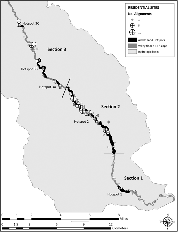
To evaluate this expectation in Range Creek Canyon, hotspots for irrigation farming were identified. Lands suitable for irrigated farming were modeled as requiring alluvial deposits, adjacency to the creek, and slopes less than 12 degrees. In Range Creek Canyon, this represents the canyon floor from the creek to the colluvial deposits adjacent to the canyon walls. Within this universe, the canyon bottom was divided into sections ranging from small to large contiguous expanses of farmable land using focal statistics in ArcGIS 10.1 (Boomgarden Reference Boomgarden2015:112-113). Five hotspots in three sections of Range Creek Canyon scored high on this scale (Figure 9). Hotspot 2 (Section 2) is the largest, with 306 ha of contiguous arable land. Given the experimental findings on the costs of irrigation reported here, we expect Fremont farmers to have preferred this area for irrigation to the alternatives because of the potential to minimize irrigation costs.
Map showing the total farmable area in hectares for arable land hotspots within three sections of Range Creek Canyon. The density and distribution of surface structures are shown in relation to canyon sections and arable land hotspots identified using focal statistics in ArcMap 10.1 (Boomgarden Reference Boomgarden2015).

The largest number of residential sites adjacent to the canyon floor in Range Creek Canyon are found in Hotspot 2 (Boomgarden Reference Boomgarden2015: 182-183). Of the 92 residential sites recorded in the main canyon, 51 are located in Hotspot 2 (Supplemental Table 1). These sites are also larger than those recorded in other sections of the canyon (average size 2,928 m2). Hotspot 2 contains more sites, with two or more rock alignments (surface structures) per site (Supplemental Table 1). Assuming that site size and number of structures correlates with population density or length of occupation (Kent Reference Kent1992), then Section 2 was more densely populated or was populated for a longer period than other areas of the canyon, indicating that it was a preferred location for settlement. Future work will more thoroughly evaluate the significance of this pattern by including estimates of the seasonal and spatial variation in creek flow, as well as variation in such factors as soil texture and nutrients along the canyon bottom.
Conclusions
We have demonstrated that the relationship between soil moisture and maize yield is a diminishing-return function where, within limits, additional moisture results in additional grain yield. Discussion of the minimum amount of moisture required to raise maize is unproductive. Irrigation should be examined as a potential strategy in areas that do not receive sufficient rainfall to attain the maximum maize yield. Whether it is a viable strategy depends on the costs and benefits of irrigating in that area. We examine one of the simplest cases, where the presence of a reliable source of permanent surface water, in this case Range Creek, can be diverted to field locations to make up that deficit between rainfall and the moisture needed to achieve higher crop yields. Based on a simple optimality model, we argue that both the benefits and costs of irrigating must be taken into consideration to evaluate whether irrigation strategies are economically viable, and if so, how much effort should be devoted to water management.
We conducted a series of experiments to collect data concerning the costs and benefits of simple diversion irrigation. A host of problems from the start, including crop damage from grasshoppers, rabbits, raccoons, horses and flash floods, plagued these experiments. We had to learn how to dig ditches with sharpened sticks, bark scoops, and our bare hands. We initially made decisions about how much effort should be put into any task that goes into building and using an irrigation system without the experience necessary to inform those decisions. For example, deciding how much effort to put into building a simple diversion dam requires an understanding of the relationship between the level of investment, the efficiency of the dam at diverting water, and its ability to survive a flood. There is also the question of the relationship between what we have called capital costs and operating costs. In a manner analogous to that described by Ugan and colleagues (Reference Ugan, Bright and Rogers2003) and Bettinger and colleagues (Reference Bettinger, Winterhalder and McElreath2006), additional investments in capital costs may decrease operating costs, and this presents its own set of intriguing trad-eoffs that deserves investigation. Because of these issues, we are still modifying the experimental protocol to generate a more accurate and complete picture of the costs and benefits of irrigation.
The focus of our research has been largely on the costs and benefits of diversion irrigation. It does not speak directly to the question of whether it is best to farm or hunt and gather wild resources in a particular setting. Answering that question requires additional research into the costs and benefits of the other farming activities, as well as the average return rates for hunting and gathering. It is tempting to use other sources of quantitative data to fill in the blanks in our data. In her compilation of selected farming ethnographic studies, Barlow (Reference Barlow2002) synthesizes the data on the costs and benefits from a number of Latin American communities. Based on these data, Barlow suggests that farmers who invest less time in their fields, especially in more productive settings, are likely to have higher return rates than those who spend more time. Barlow equates this to Boserup's (Reference Boserup1965) definition of intensification, where more time (labor) invested in farming increases productivity but results in a decrease in farming efficiency. In other words, intensification leads to a decrease in the rate of return for farming or other subsistence pursuits (Morgan Reference Morgan2015).
In light of the OIM, intensification occurs when irrigation exceeds y opt, reducing the rate of return but increasing the yield per unit area (up to y max). Time spent irrigating at or below y opt increases the yield per unit area, but also increases the rate of return. This is not intensification according to Boserup's definition. We expect that experienced farmers understand the relationships between time spent in various farming activities and expected size of harvest. Irrigation can require substantial costs, but our analysis highlights when those costs are more than offset by increased benefits. The presence of features associated with prehistoric irrigation does not necessarily indicate intensification (not without additional evidence). Equally important, sources of ethnographic or experimental farming data that do not examine the relationship between costs and benefits of the farming activity in the setting in which they were collected must be viewed with caution.
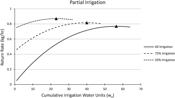
Our research provides several general implications for historic and prehistoric farming. First, even when farming without irrigation can produce significant harvests, irrigation may still improve the efficiency of farming. Figure 10 illustrates the return-rate functions of irrigation derived from the 2017 cost data (see Figure 8b). The lower function (solid line) illustrates the case when all the soil moisture is derived from irrigation. The upper functions illustrate the return rate when irrigation provides only some of the moisture. In each case examined, providing supplemental water through irrigation is expected, even when there is significant growing-season precipitation. The maximum (optimal) return rates also increase as the amount of irrigation decreases because available water is modeled as having no cost. We would expect that as average rates of return for hunting and gathering decline in a region, hunter-gatherers living in areas where smaller quantities of irrigation water are needed will begin farming before similar populations in areas where the need is greater.
Illustration of the effects of different irrigation requirements using 2017 cost data. For 50% irrigation, 50% is provided by rainwater, 50% from irrigation. Irrigation is expected in all three scenarios. Triangles indicate the optimal return rates.

Second, by definition, irrigation always incurs costs. Therefore, the optimal time spent irrigating will always be less than the amount of time required to produce the maximum yield. All else being equal, the higher the operating costs, the greater the difference between optimal and maximum irrigation, and conversely, the lower the costs, the lower the difference. We modeled the operating costs as independent of the capital costs of irrigation, which is undoubtedly an unrealistic assumption. Given the model, the capital costs are important for determining the maximum rate of return for irrigating, which influences how it compares to the expected return rates for hunting and gathering.
Third, the costs and benefits for irrigation are partially a function of local environment and, especially with respect to costs, are likely to vary from one local area to another. This should not deter future research into the economics of farming because we are optimistic that useful generalizations will become apparent as further problem-oriented research is completed in other environmental settings. The research presented here provides the theoretical and methodological foundations to conduct and critically compare additional cases.
Acknowledgments
This work was made possible by the support of the Natural History Museum of Utah and the Department of Anthropology, University of Utah. Earlier drafts benefited from the comments of Brian Codding and the UUAC lab group. Liz Baldwin, Joel Boomgarden, Jack Broughton, Larry Coats, Joan Coltrain, Isaac Hart, Kristen Hawkes, Michelle Knoll, Dave Potter, Frances Metcalfe, James O'Connell, and Corinne Springer provided comments, edits, and support. We would like to thank the dozens of field school students who assisted with data collection over the years. This paper greatly benefitted from constructive comments from Robert Kelly, Lynn Gamble, and five anonymous reviewers. Thanks to Fanny Guadalupe Blauer for translating the English abstract to Spanish.
Data Availability Statement
Additional methods, datasets, and details of early experiments are available in Boomgarden Reference Boomgarden2015, Experimental Maize Farming in Range Creek Canyon, Utah. The physical and digital data from which this research is based is curated at the Natural History Museum of Utah, University of Utah, Salt Lake City.
Supplemental Materials
For supplementary material accompanying this paper, visit https://doi.org/10.1017/aaq.2018.90
Supplemental Figure 1. Graphic illustration of the growing season variation in the daily water needs of modern hybrid maize in Nebraska. The greatest evapotranspiration occurs when the plant produces tassels, and the least is just after plant emergence.
Supplemental Figure 2. Photographs from water-crop production experiment documenting water stress (left) a basin in Plot 2 irrigated once every two weeks and (right) a basin in Plot 4 irrigated twice per week. Both photographs were taken on July 23, 2014.
Supplemental Figure 3. Graph showing decadal precipitation reconstruction from the Harmon Canyon dendrochronology sequence, Nine Mile Canyon (Boomgarden Reference Boomgarden2015:179 based on Knight et al. Reference Knight, Meko and Baisan2010:Figure 6:5b). Departures above and below the mean (38 cm) show extremely wet and dry periods defined as Gaussian-filtered series with standardized values greater than 1.25 in absolute values (Knight et al. Reference Knight, Meko and Baisan2010).
Supplemental Text 1. Key References Consulted about Archaeologically, Experimentally, and Ethnographically Documented Farming Techniques.
Supplemental Text 2. Key References Consulted about the Water-Crop Production Function and Deficit Irrigation.
Supplemental Table 1. Residential Site Distribution Summary.