Nomenclature
- Nb
-
blade numbers
- V
-
wind speed /m/s
- Ω
-
rotor speed/rpm
- α
-
tilt angle /°
- R
-
blade length/m
-
 ${\theta _{{\rm{0}}{\rm{.7}}}}$
-
collective pitch/°
- e
-
flapping hinge offset/m
-
${\theta _C}$
-
lateral cyclic pitch/°
-
${K_\beta }$
-
flapping hinge spring stiffness n.m/rad
-
${\theta _S}$
-
longitudinal cyclic pitch/°
-
${K_\lambda }$
-
pitch-flap coupling coefficient
- c
-
chord/m
-
${I_\beta }$
-
flapping moment of inertia/kg.m2
-
${C_L}$
-
lift coefficient of aerofoil
- σ
-
rotor solidity
-
${C_D}$
-
drag coefficient of aerofoil
-
$\bar v$
-
induced velocity/non-dimensionalisation
-
${C_M}$
-
pitching moment coefficient
-
$\bar r$
-
radial position/ non-dimensionalisation
- CT
-
rotor thrust coefficient (axial)
-
$\psi $
-
azimuth
- CQ
-
shaft torque coefficient
- k
-
induced inflow factor
- FD
-
Fréchet distance
-
$\rho$
-
density/ kg/m3
-
$\beta$
-
flapping angle/°
- μ
-
helicopter advance ration
- J
-
axial flow advance ratio
-
${\lambda _0}$
-
time-averaged inflow component
-
${\lambda _{1c}}$
-
first-order longitudinal inflow component
-
${\lambda _{1{\rm{s}}}}$
-
first-order lateral inflow component
-
$U$
-
resultant speed/ m/s
-
${M_A}$
-
aerodynamic torque
-
${M_{CF}}$
-
centrifugal torque
-
${M_I}$
-
inertial torque
-
${M_{C{\rm{or}}}}$
-
Coriolis torque
-
${M_R}$
-
flapping constraint torque
-
${M_{BA}}$
${M_{BL}}$
-
additional torque
- APPDI
-
augmented Pitt-Peters dynamic inflow model
- BET
-
blade element theory
- GA
-
genetic algorithm
- FA
-
fmincon algorithm
-
$\dot{[\ ]}$
-
Take the derivative with respect to time


1.0 Introduction
The design of flight control system for tiltrotor aircraft requires real-time and accurate aerodynamic load inputs. While high-fidelity methods such as computational fluid dynamics (CFD) [Reference Oyama and Rostami1, Reference Bernardini, Centracchio and Gennaretti2] and free-wake methods [Reference Iannotta, Visingardi and Quagliarella3, Reference Sebastian and Lackner4] can resolve complex flow fields in detail, their substantial computational cost prevents their use in the rapid iteration cycles of flight control design [Reference Peters and HaQuang5]. For real-time simulation and control design, the prevailing approach employs a coupled framework that combines the Pitt-Peters dynamic inflow model [Reference Peters and HaQuang5, Reference Murakami and Houston6] with blade element theory (BET). In this framework, the dynamic inflow model solves the induced velocity distribution at the rotor disk, and BET is then used to integrate the aerodynamic forces along blade elements. This methodology balances computational efficiency with acceptable accuracy, and it often serves as the baseline model for control law design and analysis [Reference Oktay and Sultan7].
Advanced tiltrotor blades are constructed with multiple aerofoil sections, making it difficult to obtain precise aerodynamic parameters – especially in the transitional regions between different aerofoils along the blade span. Due to this limitation, the more accurate semi-empirical unsteady aerodynamic models (e.g. ONERA [Reference Gaonkar and Peters8], Leishman-Beddoes [Reference Boutet, Dimitriadis and Amandolese9]) cannot be directly applied. Consequently, BET must rely on interpolated aerofoil data, which introduces inherent inaccuracies at the input stage. These input errors lead to significant uncertainties in predicting induced velocity, particularly during complex manoeuvres like dynamic tilting. These limitations restrict the framework’s ability to provide reliable inputs for advanced flight control systems.
Current research aims at enhancing aircraft performance under model uncertainty focuses on two main areas. The first area is airframe-control co-design and active intervention, which involves optimising or dynamically altering the aerodynamic geometry. Examples include the simultaneous stochastic optimisation of small unmanned aerial vehicle (SUAV) control surfaces, powerplant system, and its automatic flight system (AFS) [Reference Yesilbaş10], as well as the co-design of vertical tail and flight control parameters [Reference Yesilbaş, Özgür, Ozen and Oktay11]. Some studies introduce active morphing technologies, such as adjusting active wing geometry [Reference Oktay, Konar, Mohamed, Aydin, Şal, Onay and Soylak12, Reference Kocamer, Kose, Sal and Oktay13] or rotor blade parameters [Reference Oktay and Sultan14, Reference Sal15], combined with optimisation algorithms to tune controllers for improved stability and energy efficiency [Reference Oktay16, Reference Kose, Oktay and Özen17]. Other research integrates active flow control (e.g. plasma actuators [Reference Ünal, Öz, Ünal and Oktay18]) with flight control system design for morphing unmanned aerial vehicles (UAVs) into a co-design scheme [Reference Kanat, Karatay, Köse and Oktay19]. The second area involves the development of advanced robust and safety-critical control theories, aiming to design controllers that suppress uncertainties and ensure safety, such as variance-constrained control [Reference Oktay and Sultan7]. Recently, for systems with uncertainties and faults, methods like fixed-time safety-critical control [Reference Gao, Liu, Bi and Yang20], reliability-constrained interval sliding mode control [Reference Yang, Liu and Gao21] and interval linear quadratic tracking control [Reference Yang, Zuo, Lu and Wang22] have emerged. These methods seek to provide strict guarantees on settling time and safety reliability.
Both the objective functions for co-design optimisation and the design process of advanced controllers, including verification and gain tuning, critically depend on high-precision aerodynamic model inputs. If the foundational model suffers from input defects due to missing aerofoil data, the reliability of any subsequent flight control design will be compromised.
Consequently, this paper is dedicated to addressing the thrust prediction deviation caused by missing input data within the computational framework coupling the Pitt-Peters dynamic inflow model with BET. This paper proposes a model parameter correction method based on wind tunnel test data for tiltrotors. In this method, an induced inflow factor k is introduced and defined as the key corrective variable to modify the rotor disk plane induced velocity. The innovations of this work are summarised as follows: first, for rotor forward flight at a fixed tilt angle, the identification of the parameter k is formulated as an optimisation problem and efficiently calibrated to improve static prediction accuracy. Second, for the continuous rotor tilting process, a time-varying quadratic function model for the parameter k is established for the first time, incorporating the direction of rotation. Third, the Fréchet distance [Reference Fréchet23] is introduced as a fitting criterion, enabling the accurate reconstruction of the aerodynamic hysteresis loop phenomenon. This wind tunnel test-driven correction method compensates for the inherent input deficiency in the classical framework, thereby providing a more reliable foundation for aerodynamic load calculation in tiltrotor flight control design.
The paper structure is as follows: Section 2 presents the parameters of the rotor and the measurement platform. Section 3 introduces the construction of the augmented Pitt-Peters dynamic inflow model and compares simulation results with experimental data. Based on Section 3 and using wind tunnel experimental data, Section 4 employs several identification methods to determine the parameters of the induced inflow factor k under different flight attitudes, thereby improving the model accuracy. Finally, Section 5 summarises the work and presents concluding remarks.
2.0 Test subjects and principles
2.1 Wind tunnel test setup
The experiments were conducted in the 8 × 6 m test section of a wind tunnel at the China Aerodynamics Research and Development Center (CARDC). The tiltrotor model was installed on a six-component strain-gauge balance for measurement of aerodynamic forces and moments. All data were recorded at a sampling frequency of 5,000 Hz using Donghua test system.
2.2 Rotor test stand
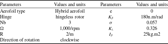
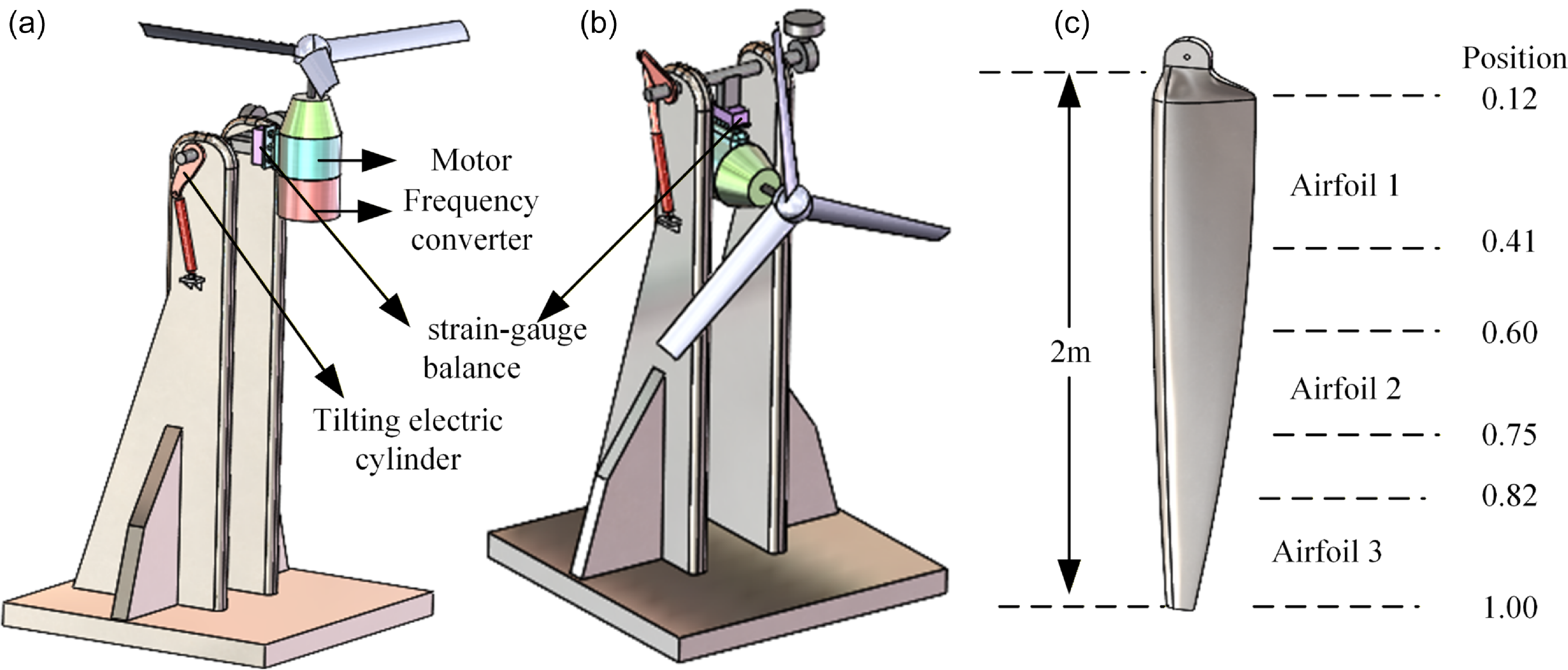
As shown in Fig. 1 (a)–(b), the rotor test stand consists of a power system, a measurement system and a tilting system. The power system employs an integrated distributed electric propulsion architecture, which includes a motor and a frequency converter. Load measurement is carried out by a six-component strain-gauge balance. The tilting system is driven by a tilting electric cylinder to achieve tilt motion, allowing the rotor to be positioned at different tilt angles for isolated wind tunnel tests. Figure 1(c) and Table 1 present the basic parameters of the rotor blades under test. The blades described in this paper consist of multiple aerofoil sections.
Rotor structure parameters

Rotor test stand and blade: (a) helicopter model (tilt angle = 90°); (b) fixed-wing model (tilt angle = 0°); (c) blade aerofoil distribution.

3.0 Dynamic inflow calculation model of the rotor
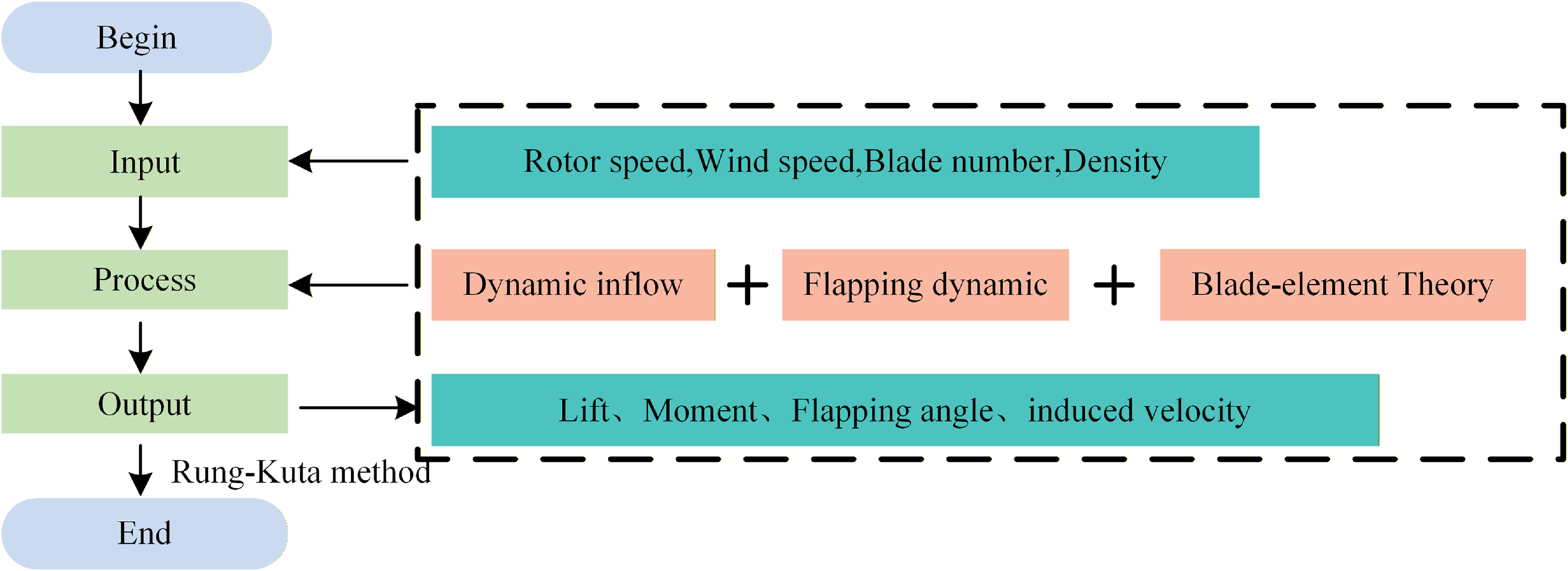
As shown in Fig. 2, the augmented Pitt-Peters dynamic inflow (APPDI) model is composed of three parts: the rotor flapping dynamics, the inflow model and the aerofoil aerodynamic model. In the dynamic inflow model, an augmented term accounting for wake distortion effects is incorporated into the traditional Pitt-Peters framework to better represent the wake behaviour under tilted operating conditions. Moreover, the classic blade-element theory is employed as the aerodynamic model to calculate the solution of the lift or torque of the rotor under different flight attitudes.
Augmented Pitt-Peters dynamic inflow model (APPDI model).

3.1 Augmented dynamic inflow model of rotor
The Pitt-Peters dynamic inflow model relates the aerodynamic and induced velocity changes due to flapping motions through a set of linear differential equations.
 \begin{align}&\qquad \bar v\left( {\bar r,\psi } \right) = {\lambda _0} + {\lambda _{1c}}\cos \psi + {\lambda _{1{\rm{s}}}}\sin \psi \end{align}
 \begin{align}& \left[ M \right]\mathop {\left[ {\begin{array}{*{20}{c}}{\Delta {\lambda _0}}\\{\Delta {\lambda _{1s}}}\\{\Delta {\lambda _{1c}}}\end{array}} \right]}\limits^ \bullet + \left[ V \right]{\left[ {\tilde L} \right]^{ - 1}}\left[ {\begin{array}{*{20}{c}}{{\lambda _0}}\\{{\lambda _{1s}}}\\{{\lambda _{1c}}}\end{array}} \right] = \left[ {\begin{array}{*{20}{c}}{CT}\\{CL}\\{CM}\end{array}} \right] \end{align}
 $\bar v$
represents the induced velocity,
 $\left[ V \right]$
is the mass flow parameter matrix,
 $\left[ {\tilde L} \right]$
matrix reflects the static relationship between the perturbed induced velocity and the perturbed aerodynamic loads and
 $\left[ M \right]$
matrix reflects the influence of air inertia, which represents the time delay of the inflow; CT, CL, CM are the coefficients of the rotor thrust, roll moment and pitching moment, respectively.
The blade mentioned in Section 2 is a multi-aerofoil spliced blade; therefore, the thrust, drag and pitching moment generated by the rotor can only be calculated using BET.
 \begin{align} dL &= \frac{1}{2}\rho {U^2}c{C_L}dr \end{align}
 \begin{align} dD &= \frac{1}{2}\rho {U^2}c{C_D}dr \end{align}
 \begin{align} dM &= \frac{1}{2}\rho {U^2}{c^2}{C_M}dr \end{align}
In BET, the blade is divided into many small segments, each element has a length of
 $dr$
. The parameters
 $dL$
,
 $dD$
and
 $dM$
represent the lift, drag and pitching moment of the blade element, respectively; c represents the chord length of the aerofoil section; U represents the resultant velocity.
 ${C_L}$
,
 ${C_D}$
and
 ${C_M}$
represent the lift coefficient, drag coefficient and pitching moment coefficient of the aerofoil, respectively, which are obtained by interpolating the aerodynamic performance table.
Based on Equation (2), the APPDI model [Reference Gaonkar and Peters8] incorporates the variation in axial inflow caused by rotor wake distortion during rotor tilting flight, yielding the following equation:
 \begin{align}& \left[ M \right]\mathop {\left[ {\begin{array}{*{20}{c}}{\Delta {\lambda _0}}\\{\Delta {\lambda _{1s}}}\\{\Delta {\lambda _{1c}}}\end{array}} \right]}\limits^ \bullet + \left[ V \right]{\left[ L \right]^{ - 1}}\left[ {\begin{array}{*{20}{c}}{\Delta {\lambda _0}}\\{\Delta {\lambda _{1s}}}\\{\Delta {\lambda _{1c}}}\end{array}} \right] = \left[ {\begin{array}{*{20}{c}}{{C_{Ta}}}\\{ - {C_{La}}}\\{ - {C_{Ma}}}\end{array}} \right] \end{align}
 \begin{align}& \left[ L \right] = \left[ {\tilde L + \Delta L} \right] = \left[ {\tilde L} \right] + \left[ {\Delta {L_1}} \right] + \left[ {\Delta {L_2}} \right] + \left[ {\Delta {L_3}} \right] \end{align}
Matrix
 $\Delta {L_1}$
represents the coupling between the wake bending and the rotor blade time-averaged loads,
 $\Delta {L_2}$
reflects the coupling effect between wake bending, tilt and blade time-averaged loads, while
 $\Delta {L_3}$
expresses the coupling tendency between wake bending, tilt and blade cycle loads.
During the rotor tilting flight, the bending, tilting and spacing changes of the dynamic wake form a system that evolves with variations in rotor disk inflow and time. The inertial effects of this system can be captured by time constants. Consequently, the influence of dynamic wake distortion on rotor disk inflow can be described by a set of first-order differential equations:
 \begin{align}\left[ {{\tau _D}} \right]\mathop {\left[ {\begin{array}{*{20}{c}}X\\S\\{{K_c}}\\{{K_s}}\end{array}} \right]}\limits^ \bullet + \left[ {\begin{array}{*{20}{c}}X\\S\\{{K_c}}\\{{K_s}}\end{array}} \right] = {\left[ {\begin{array}{*{20}{c}}X\\S\\{{K_c}}\\{{K_s}}\end{array}} \right]_{qs}}\end{align}
In Equation (8) [Reference Gaonkar and Peters8],
 $X$
,
 $S$
,
 ${K_C}$
,
 ${K_S}$
represent the tilting spacing variation, longitudinal and lateral wake curvature effects of the wake, respectively. The subscript ‘qs’ denotes quasi-steady values, the matrix
 $\left[ {{\tau _D}} \right]$
contains the time constants related to the dynamic wake distortion effects.
3.2 Dynamic model of rotor flapping
When a tiltrotor undergoes continuous tilting, additional angular motions such as roll and pitch influence the rotor’s flapping response. In consideration of the aerodynamic environment during dynamic tilting, the blade dynamics must account for the effects of Coriolis and inertial forces.
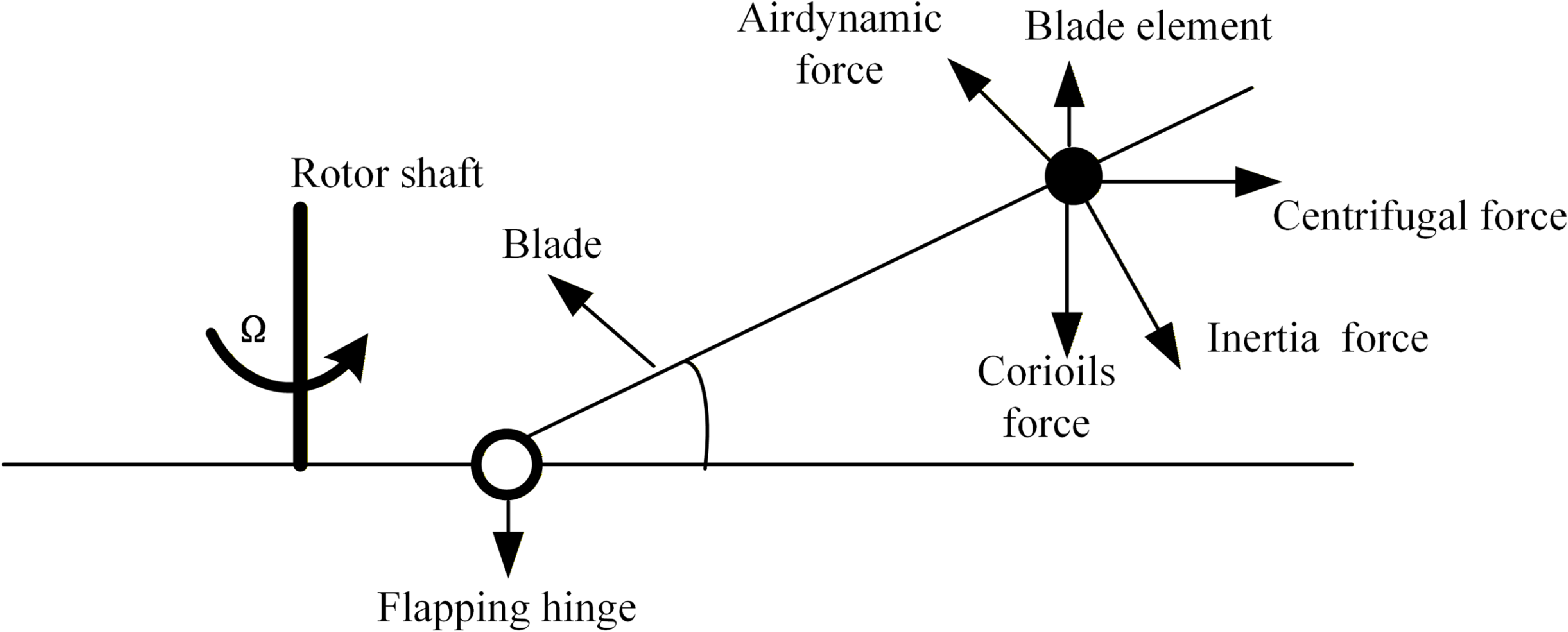
As shown in Fig. 3, the flapping dynamic equation is formulated within the single-blade coordinate system based on moment equilibrium at the flapping hinge, with blade weight being neglected.
 \begin{align}&\qquad {M_A} + {M_{CF}} + {M_I} + {M_{Cor}} + {M_R} + {M_{BA}} + {M_{BL}} = 0 \end{align}
 \begin{align}&\qquad\qquad {M_{CF}} = - {\Omega ^2}\left( {{I_\beta }\cos \beta + e{M_b}} \right)\sin \beta \end{align}
 \begin{align}&\qquad\qquad\qquad\qquad\quad {M_I} = - {I_\beta }\ddot \beta \end{align}
 \begin{align}& {M_{Cor}} = 2\left( {{I_\beta }{{\cos }^2}\beta + {e_b}{M_b}\cos \beta } \right)\left( {{p_h}\Omega \cos \psi - {q_h}\Omega \sin \psi } \right) \end{align}
 \begin{align}&\qquad\qquad\qquad\qquad\quad {M_R} = - {K_\beta }\beta \end{align}
 \begin{align}&\quad\,\, {M_{BA}} = \left( {{I_\beta }{{\cos }^2}\beta + e{M_b}\cos \beta } \right)\left( {{{\dot p}_h}\sin \psi + {{\dot q}_h}\cos \psi } \right) \end{align}
 \begin{align}&\quad {M_{BL}} = {M_B}\left( {\cos \beta {a_{hz}} - \sin \beta {a_{hx}}\cos \psi + \sin \beta {a_{hy}}\sin \psi } \right) \end{align}
Rotor blade flapping motion model.

Here,
 ${M_A}$
is the aerodynamic torque acting on the blade,
 ${M_{CF}}$
is the centrifugal torque,
 ${M_I}$
is the inertial torque,
 ${M_{Cor}}$
is the Coriolis torque,
 ${M_R}$
is the constraint torque caused by the flapping hinge,
 ${K_\beta }$
is the flapping spring coefficient,
 ${M_{BA}}$
is the torque caused by the angular acceleration of the hub centre,
 ${a_{hx}}$
,
 ${a_{hy}}$
and
 ${a_{hz}}$
are the linear accelerations of the hub centre,
 ${p_h}$
and
 ${q_h}$
represent the roll and pitch rate of the rotor hub,
 ${M_{BA}}$
and
 ${M_{BL}}$
are the additional torque.
3.3 Calculation of rotor thrust
By using the ODE45 method, the system of differential equations comprising Equations (8) and (9) is solved to compute the rotor loads, including induced velocity, forces and moments. The rotor loads for hovering, fixed-tilt forward flight and dynamic tilt conditions are computed based on the rotor parameters listed in Table 1. The rotor performance is evaluated in terms of the rotor thrust coefficient (axial) (CT) and shaft torque coefficient (CQ) and compared with experimental data. To further validate the model, publicly available experimental data for hovering, helicopter forward flight and axial flow conditions are additionally introduced. All numerical solutions are obtained using the MATLAB 2022 solver over a time duration of 10 seconds.
3.3.1 Hovering state
To validate the effectiveness of the proposed method, the model described above is verified using the publicly available hover experimental data from Ref. [Reference Caradonna and Tung24]. The verification results are shown in Fig. 4.
As illustrated in Table 2 and Fig. 4, the APPDI model employed in this study demonstrates a high degree of consistency between the simulation results and experimental data when predicting the rotor hover load, indicating its effectiveness in accurately capturing the aerodynamic performance under hovering conditions.
Hovering load of validation dataset

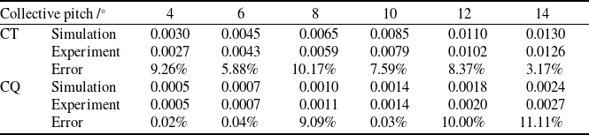
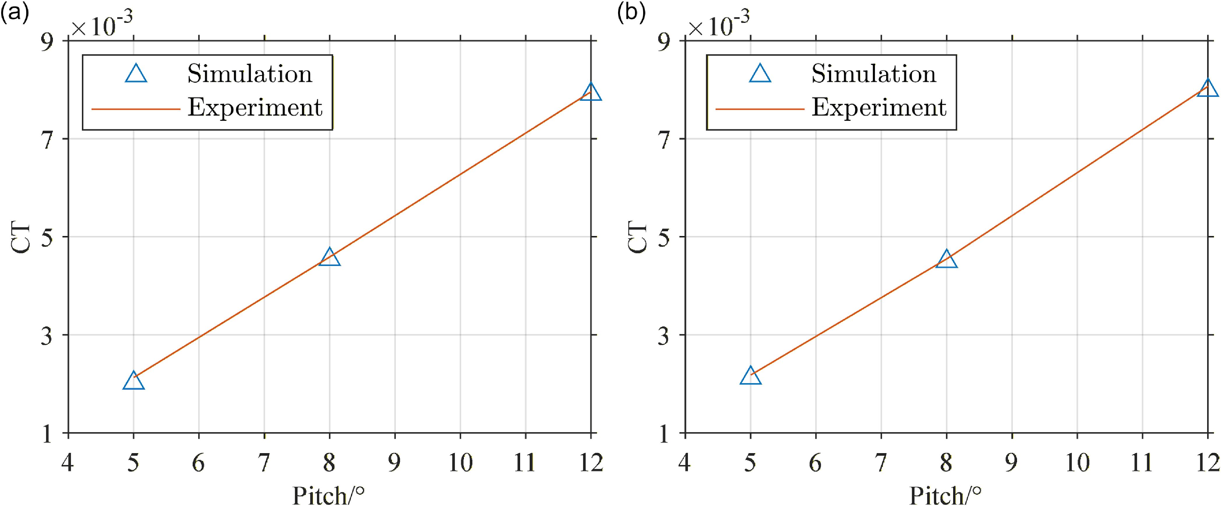
Based on the experimental setup described in Section 2, hover performance tests were conducted. As shown in Table 3, the measured load distributions across a range of collective pitch angles – from 4° to 14° – are compared with computed results.
Hovering load distribution

Hover performance at different collective pitch settings: (a) CT distribution of 1,250 rpm; (b) CT distribution of 1,750 rpm.

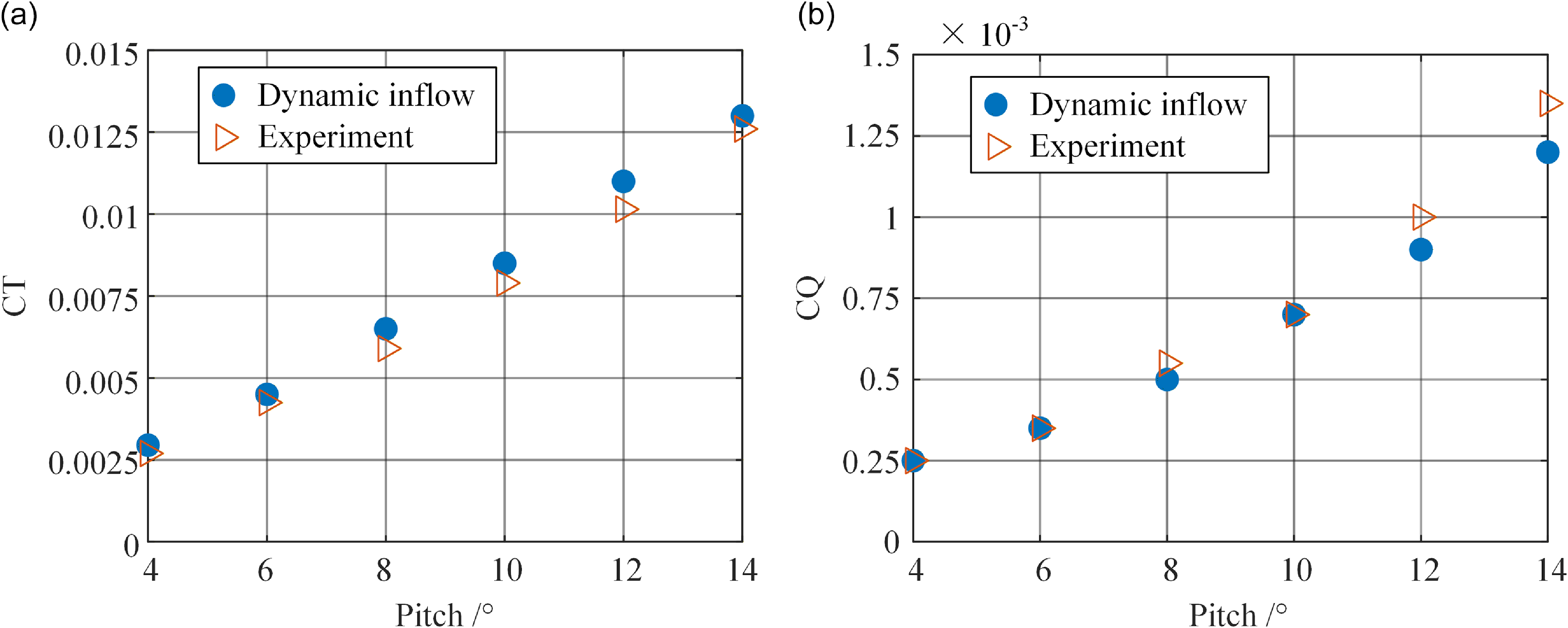
As seen from Table 3 and the variation curves of CT and CQ with collective pitch shown in Fig. 5(a)–(b), the calculation results of the augmented dynamic inflow model are in good agreement with the experimental results indicating that this model can be effectively applied to the evaluation of the hovering loads of rotors in practical engineering.
Hover performance at different collective pitch settings: (a) CT distribution; (b) CQ distribution.

3.3.2 Forward flight with fixed title angle state
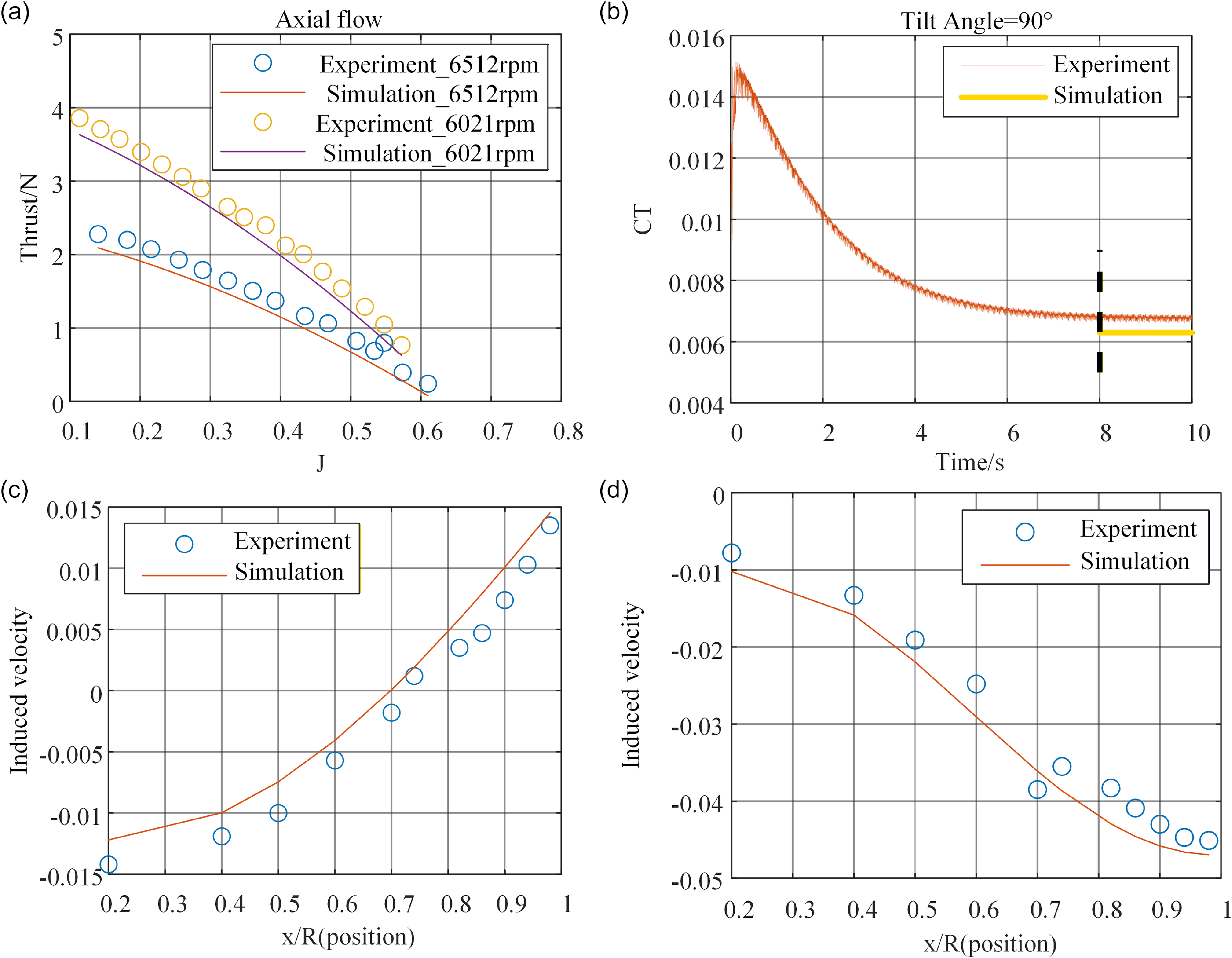
To further verify the effectiveness of the method in this paper, the above model was validated using the helicopter forward flight experimental data and axial flow experimental data published in the Refs [Reference Elliott, Althoff and Sailey25–Reference Theys, Dimitriadis, Andrianne, Hendrick and De Schutter27].
As shown in Fig. 6(a) for the axial flow condition, the CT decreases with increasing axial flow advance ratio
 $J={{\Omega \cdot V \cdot \pi } \over {{\rm{60}} \cdot {\rm{R}}}}$
under different rotational speeds. The simulation results show good agreement with experimental data, indicating that the proposed model is suitable for thrust prediction in axial flow. Figure 6(b) reveals a slight deviation between simulated and experimental CT values (helicopter advance ratio
 $\mu ={{V \cdot \cos \alpha \cdot {\rm{30}}} \over {\Omega \cdot {\rm{R}} \cdot \pi }}$
). However, the induced velocity distributions at different azimuth angles in Fig. 6(c)–(d) exhibit consistent trends. Therefore, the APPDI model remains effective for CT prediction in helicopter forward-flight mode.
Hover performance at different collective pitch settings: (a) thrust distribution at different advance ratio J; (b) CT of rotor at μ = 0.15; (c) induced velocity at azimuth angle ψ = 180°; (d) induced velocity at azimuth angle ψ = 330°.

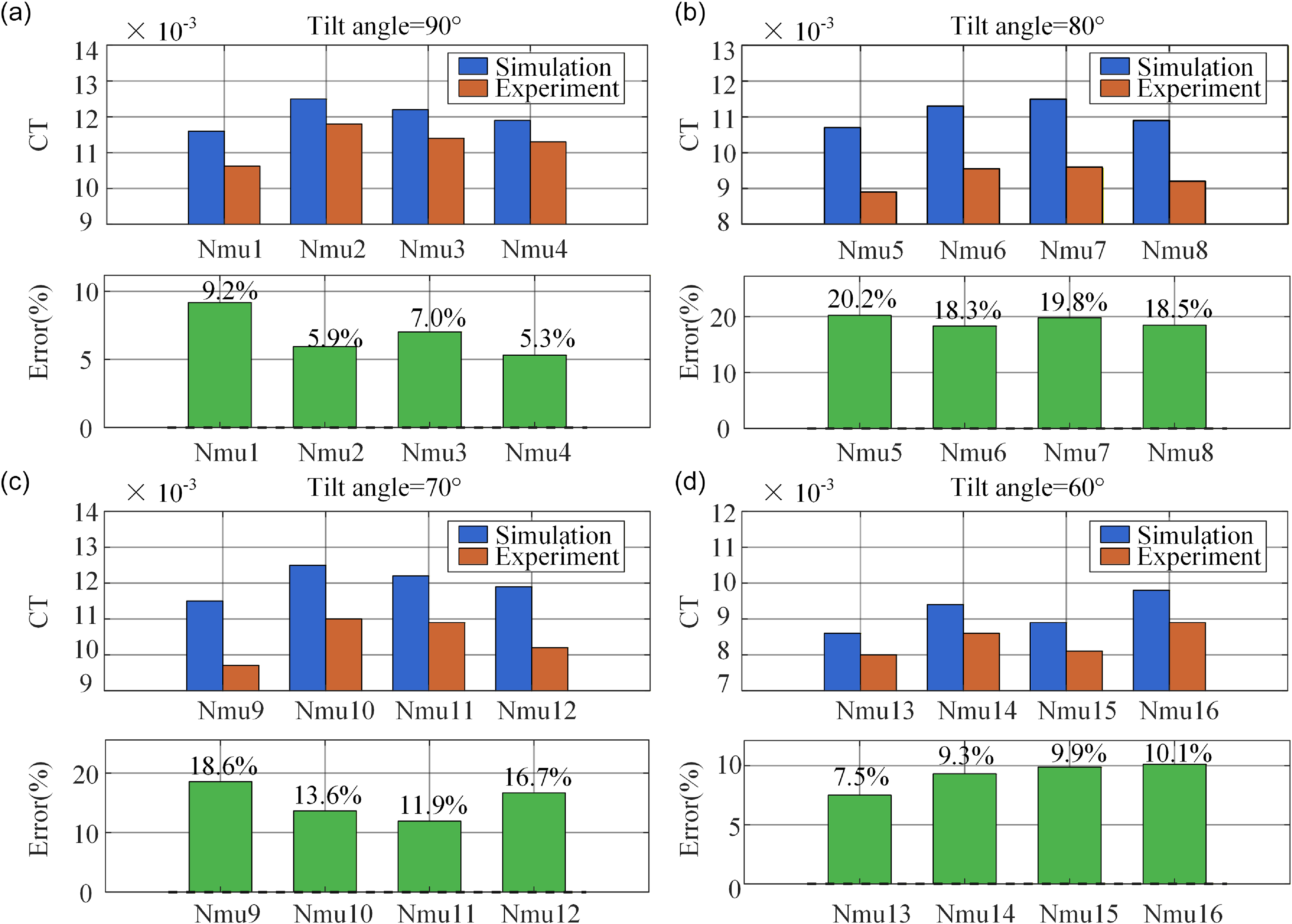
Meanwhile, wind-tunnel test data for an isolated tiltrotor at different tilt angles were collected using the test stand described in Section 2, with the control angles measured during the experiment then used as input for the simulation model.
Figure 7(a)–(d) shows that the maximum error of simulation model is 20%, while the minimum is 5.3%. The overall error for the four test cases at an 80° tilt angle is higher than that at other tilt angles. Overall, the simulations capture the general aerodynamic trends effectively. The observed discrepancies can be attributed to the following factors:
-
1. The actual control inputs in flight result from aeroelastic trim, whereas simulation model treats the blades as rigid, introducing simplification errors.
-
2. The wake undergoes significant bending at different tilt angles, intensifying blade–vortex interactions and three-dimensional aerodynamic interference among blades. The blade-element theory cannot fully capture these effects.
-
3. The aerodynamic coefficients of the blended aerofoil sections are obtained via interpolation, which may deviate from the actual complex flow behaviour.
These factors collectively lead to inaccuracies in the prediction of induced velocity
 $\bar v$
, which is the core source of the discrepancies between simulations and experiments.
3.3.3 The continuous tilting process
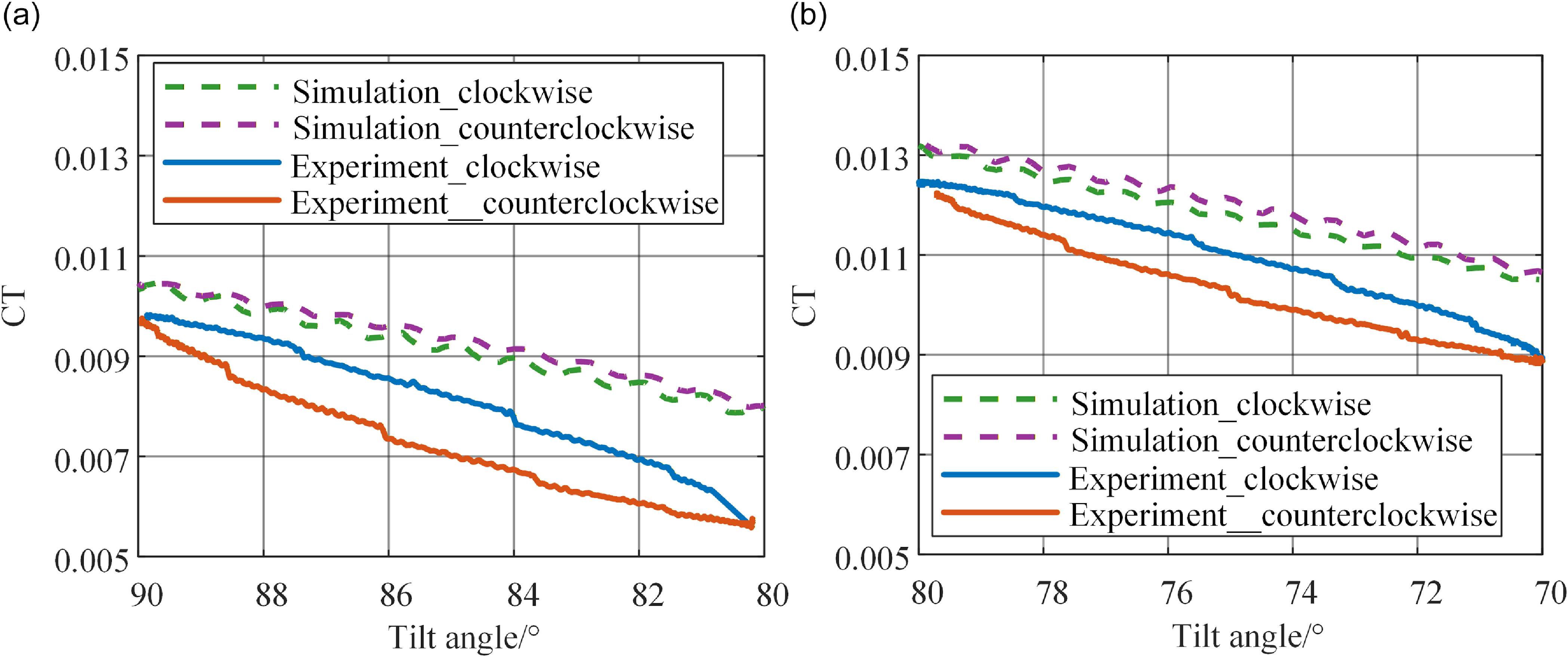
The continuous tilting process, defined as the rotor’s continuous motion between two specified tilt angles, is examined in two test cases shown in Table 4. In this study, a decrease in the tilt angle is defined as clockwise rotation, while an increase is defined as counterclockwise rotation. For the simulations, the control angle inputs are set directly based on the actual measured values from the corresponding experimental cases listed in Table 4. Throughout the continuous tilting process, these control angles were held constant.
Figure 8(a)–(b) shows that the simulation model successfully captures the general trend of the CT during continuous tilting. CT decreases during clockwise rotation (decreasing tilt angle) and increases during counterclockwise rotation (increasing tilt angle), consistent with the experimental data. This indicates the simulation model’s effectiveness in predicting the qualitative load variations. However, a significant discrepancy exists between the simulation results and experiment results, with a maximum error of 34.4%. Furthermore, the simulated CT in the clockwise (decreasing-angle) phase is systematically higher than the experimental value at the same tilt angle – a discrepancy contrary to experimental observations. This deviation may be attributed to the following factors:
-
1. Structural simplification: The APPDI model is predicated on the assumption of rigid blades, thereby excluding the effects of aeroelastic coupling. In contrast, the control inputs implemented in the experimental setup inherently incorporate the dynamic behaviour of an integrated and flexible rotor system.
-
2. Aerodynamic modeling limitations: The BET is unable to fully capture the highly unsteady flow features during continuous tilting, such as those arising from wake bending, distortion and complex rotor-vortex or blade-blade interactions.
-
3. Incomplete aerofoil data: The aerodynamic data for the blade spliced sections are derived through interpolation. Moreover, the current model cannot represent dynamic stall that may occur in certain blade regions during rapid tilting.
Test conditions of wind tunnel for continuous tilting

CT and error distribution at different tilt angles: (a) tilt angle = 90°; (b) tilt angle = 80°; (c) tilt angle = 70°; (d) tilt angle = 60°.

Continuous tilting process at different tilt angles: (a) tilt angle from 90 to 80°; (b) tlt angle from 80 to 70°.

Collectively, these limitations lead to inaccuracies in predicting the induced velocity
 $\bar v$
distribution, which is the primary cause of the observed discrepancies between model predictions and experimental results.
4.0 Calculation of the rotor lift combining the identification of the induced inflow factor
The APPDI model and BET framework exhibit notable limitations when calculating the forward flight conditions of tiltrotor aircraft across different tilt angles. These limitations arise primarily from wake curvature and flow distortion, which give rise to significant unsteady aerodynamic effects. Although the Office National d’Etudes et Recherches Aérospatiales (ONERA) model and the Leishman-Beddoes (L-B) model can better capture unsteady aerodynamic behaviour, they are semi-empirical in nature and rely heavily on accurate experimental data for aerofoil sections. The blade investigated in this study features a hybrid aerofoil design, particularly in the transition regions, where essential aerodynamic parameters are not available. Consequently, conventional unsteady aerodynamic models cannot be effectively applied to such blades.
To improve computational accuracy, this study focuses on obtaining an accurate induced velocity distribution based on the foregoing analysis. An induced inflow factor k is incorporated into the induced velocity in Equation (1). This factor comprehensively represents the effects of multiple complex factors, including wake distortion and unsteady effects. Through parameter identification, the factor k can be determined at specified flight conditions, such as fixed tilt angle state and continuous tilting state. This facilitates a rapid assessment of aerodynamic loads.
 \begin{align}\bar v\left( {\bar r,\psi } \right) = k \cdot \left( {{\lambda _0} + {\lambda _{1c}}\cos \psi + {\lambda _{1{\rm{s}}}}\sin \psi } \right)\end{align}
4.1. Fixed tilt angle state
4.1.1 Identification of the induced inflow factor
To correct the induced velocity for the tiltrotor across different tilt angles, as discussed in Section 3.3.2, an optimisation problem is formulated. The objective is to identify the optimal induced inflow factor k for accurately representing the induced velocity distribution. Based on the mathematical relationship derived from solving the governing differential equations, when
 ${{\rm{F}}^{simu}}_\alpha $
<
 ${{\rm{F}}^{\exp }}_\alpha $
,
 ${\rm{k}} \in \left( {0,1} \right)$
or
 ${{\rm{F}}^{simu}}_\alpha $
>
 ${{\rm{F}}^{\exp }}_\alpha $
 ${\rm{k}} \in \left( {1,a} \right)$
. The optimisation problem, defined by its objective function and specified constraints, is then solved to obtain this optimal k.
 \begin{align*}\left\{ {\begin{array}{*{20}{c}}{{\text{min }}{{\rm{g}}_\alpha }\left( k \right) = \left\| {{{\rm{F}}^{simu}}_\alpha \left( k \right) - {{\rm{F}}^{\exp }}_\alpha } \right\|_2^2}\\{{\text{subject to }}\left\{ {\begin{array}{*{20}{c}}{k \in (0,1){\text{ if }}{{\rm{F}}^{simu}}_\alpha (k = 1) \lt {{\rm{F}}^{\exp }}_\alpha }\\{k \in (1,a){\text{ if }}{{\rm{F}}^{simu}}_\alpha (k = 1) \gt {{\rm{F}}^{\exp }}_\alpha }\end{array}} \right.}\end{array}} \right.\end{align*}
Here, k is the induced flow factor, α represents the tilt angle,
 ${{\rm{F}}^{simu}}_\alpha$
stands for the CT in the simulation state, and
 ${{\rm{F}}^{\exp }}_\alpha $
stands for the CT measured in the experiment, and a represents a constant greater than 1.
To address this parameter identification problem, this paper compares the computational efficiency of the genetic algorithm (GA) and the nonlinear constrained optimisation algorithm (fmincon algorithm, FA). The GA performs a global search through a bionic mechanism (encoding, selection, crossover, mutation), and its mathematical model can be expressed as G (C, F, P, N, S, E, M, T), where C is the encoding method, P is the initial population, N is the population size, S/E/M are genetic operators and T is the termination criterion. In contrast, FA implements local fine-tuning optimisation based on gradient information to obtain the optimal k value by minimising an objective function.
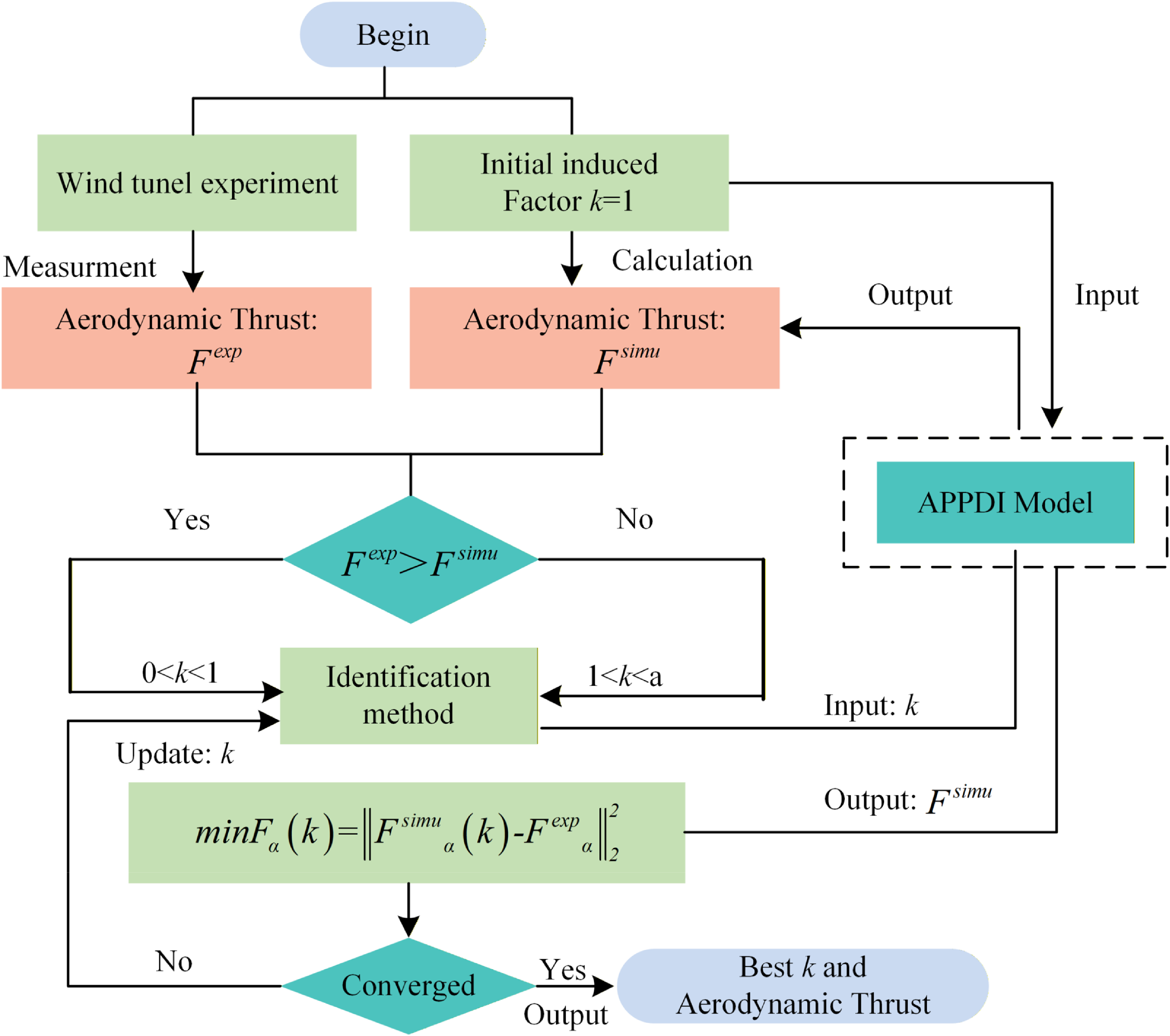
The calculation process is as follows, with the overall framework illustrated in Fig. 9:
-
1. Compute the CT when k = 1 and compare it with the CT obtained from wind tunnel experiments;
-
2. Incorporate the constraint conditions defined in Equation (16) into the identification algorithm. Update the induced inflow factor k, integrate the updated k into the APPDI model and compute the
${{\rm{F}}^{simu}}_\alpha$
. Comparing the
${{\rm{F}}^{simu}}_\alpha $
with
${{\rm{F}}^{\exp }}_\alpha $
to evaluate whether the convergence criteria are satisfied; -
3. If the convergence criteria remain unsatisfied, iteratively repeat Step 2 to refine k until the error threshold is achieved;
-
4. Upon satisfying the convergence criteria, output the optimised k, along with the
${{\rm{F}}^{simu}}_\alpha $
and induced velocity distributions.


Identification algorithm progress.

4.1.2 Analysis of parameter identification results
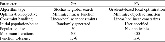
This section conducts the parameter identification of the aforementioned induced inflow factor k for fixed tilt angle in Section 3.3.2. The study employs two previously mentioned identification methods – GA and FA. The default key parameter settings of the two methods (based on MATLAB 2022a) are compared in the Table 5.
Comparison of default key parameter settings between GA and FA

As shown in Fig. 10(a), FA identifies the induced inflow factor k approximately 5–6 times faster than GA across the four tilt angles, with the highest efficiency observed at 60°. Therefore, FA can be selected as the preferred identification method for the induced inflow factor k. As illustrated in Fig. 10(b), the value of k consistently converges to 1.9 under varying values of parameter ‘a’ (representing changes in the mathematical boundary conditions). This behaviour demonstrates the strong robustness and stability of the proposed identification approach.
Comparison of identification method: (a) comparison of computational efficiency; (b) robustness verification of FA; (c) identified CT results of at different tilt angles.

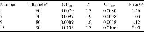
From the identified CT results presented in Fig. 10(c) and Table 6, it can be observed that after applying the identification method, the induced inflow factors under different tilt angles are successfully identified, with the calculation accuracy of the aerodynamic lift controlled within 1.2%. These results indicate that, under the fixed tilt angle conditions, the preferred FA can effectively identify the distribution of the induced flow factor k, providing a reliable solution for the modification of the subsequent calculation model and the design of the flight control system.
Identified CT results

4.2 Continuous tilting state
4.2.1 Identification of the induced inflow factor method
To describe the evolution of the induced inflow factor during the dynamic tilting process, a time-varying model for k(t) is established. The model formulation is based on the transition of the rotor tilt angle from an initial state
 ${\alpha _1}$
(corresponding to the induced inflow factor
 ${k_1}$
) to the finial state
 ${\alpha _2}$
(corresponding to an inflow ratio of
 ${k_2}$
). According to the distribution patterns of the experimental loads shown in Fig. 8, a quadratic distribution function for the induced inflow is proposed:
 \begin{align}k(t) = A \cdot {t^2} + B \cdot t + C{\rm{ }}t \in \left[ {{t_1},{t_2}} \right]\end{align}
Fréchet distance (FD) [Reference Fréchet23] is introduced as the objective function to quantify the temporal and spatial similarity between the experimentally measured CT and the simulated CT:
 \begin{align}{\rm{FD}} = \mathop {\inf }\limits_{\alpha ,\beta } \mathop {{\rm{max}}}\limits_{\tau \in \left[ {0,1} \right]} \left\| {{F_{\exp }}\left( {\alpha \left( \tau \right)} \right) - {F_{simu}}\left( {\beta \left( \tau \right)} \right)} \right\|\end{align}
where
 $\alpha \left( \tau \right)$
and
 $\beta \left( \tau \right)$
are parametric synchronisation paths of two curves. By minimising FD and satisfying the above constraints, the parameter identification problem is transformed into an identification problem with coefficient vector
 $\vec P = (A,B,C)$
:
Clockwise:
 \begin{align}\left\{ {\begin{array}{*{20}{c}}{{\text{min }}FD(P)}\\{{\text{subject to }}\left\{ {\begin{array}{*{20}{c}}{{\text{if }}\alpha ={\alpha _{\rm{1}}}{\text{ }}k({t_1}) = {k_1}{\text{ ;if }}\alpha ={\alpha _{\rm{2}}}{\text{ }}k({t_2}) = {k_{\rm{2}}}{\text{ }}t \in \left[ {{t_1},{t_2}} \right]}\\{a \gt 0; - \frac{b}{{2a}} \le {t_1};\,k({t_1}) \le k(t) \le k({t_2})}\end{array}} \right.}\end{array}} \right.\end{align}
Counterclockwise:
 \begin{align}\left\{ {\begin{array}{*{20}{c}} {{\text{min }}FD(P)} \\ {{\text{subject to }}\left\{ {\begin{array}{*{20}{c}}{{\text{if }}\alpha ={\alpha _{\rm{1}}}{\text{ }}k({t_1}) = {k_1}{\text{ ;if }}\alpha ={\alpha _{\rm{2}}}{\text{ }}k({t_2}) = {k_{\rm{2}}}{\text{ }}t \in \left[ {{t_1},{t_2}} \right]}\\ {a \lt 0; - {b \over {2a}} \le {t_1};\,k({t_1}) \le k(t) \le k({t_2})} \end{array}} \right.}\end{array}} \right.\end{align}
By integrating the FA from Section 4.1, the optimal coefficient vector
 $\vec P = (A,B,C)$
is obtained under these constraints, thereby achieving the identification of the time-varying induced inflow factor k(t) for the dynamic tilting stage.
The computational procedure is outlined as follows, with the overall framework illustrated in Fig. 11:
-
1. Based on the identification algorithm in Section 4.1, the induced factors
$k({t_1})$
and
$k({t_2})$
corresponding to the dynamic tilt the initial and final angles are calculated; -
2. The constraint conditions from Equations (18) or (19) are incorporated into the optimisation algorithm to evaluate whether the convergence criteria for the objective function are satisfied;
-
3. Output the
$\vec P = (a,b,c)$
that satisfies the specified conditions, as well as the corrected aerodynamic lift and induced velocity.


Identification algorithm progress.

4.2.2 Analysis of parameter identification results
By integrating the wind tunnel test conditions in Table 4, the FA is adopted to identify the distribution function of the induced factor under the continuous tilting conditions. A, B and C represent the coefficient of the quadratic term, the coefficient of the linear term and the constant term of the k(t), respectively.
Figures 12 and 13 and Table 7 compare the rotor thrust distribution before and after the inflow factor identification. The comparison reveals that the original simulation results exhibited a ‘hysteresis loop’ trend in both clockwise and counterclockwise loads, which is inconsistent with the experimental data. By applying the quadratic distribution function for the induced inflow factor k proposed in this study, in conjunction with the FA identification method, successfully corrected this inconsistent trend (it successfully corrected the inconsistency between experimental and simulation trends).
Comparison of simulated and experimental CT values at different tilt angles from 90 to 80°: (a) not using induced inflow factor; (b) using induced inflow factor.

This correction has significantly enhanced the accuracy. Specifically, in the 90–80° interval, the maximum error has been reduced from 34.10 to 10.70%; in the 80–70° interval, the maximum error has decreased from 18.60 to 5.55%. Using computational models, these improvements provide valuable guidance for aircraft flight control design.
Test conditions of continuous tilting

Comparison of simulated and experimental CT values at different tilt angles from 80 to 70°: (a) not using induced inflow factor; (b) using induced inflow factor.

5.0 Conclusions
This study develops a parameter identification framework for the induced inflow factor k based on the APPDI model to enhance the prediction accuracy of tiltrotor aerodynamic loads. The overall framework successfully bridges the gap between the computationally efficient APPDI model and the high-fidelity requirements of flight control design. The core innovations are threefold: first, it formulates the correction of complex inflow effects at fixed tilt angles as an optimisation problem, enabling efficient algorithmic implementation; second, it introduces a novel time-varying quadratic model for k(t) to accurately capture aerodynamic hysteresis during continuous nacelle tilting; third, it employs the FD as a fitting criterion for dynamic processes, which is validated through comprehensive wind tunnel testing. Collectively, this approach delivers a high-fidelity yet computationally efficient model suitable for flight control applications. The main quantitative findings are summarised as follows:
-
1. High-fidelity hover performance was validated. The model demonstrated excellent agreement with experimental data across a collective pitch range of 4 to 14°. The prediction error for the rotor CT ranged from a minimum of 3.17% to a maximum of 10.17%, while the error for the torque coefficient CQ ranged from 0.02 to 11.11%. These results confirm the model’s reliability for preliminary aerodynamic evaluation and load envelope analysis under hover conditions.
-
2. Load reconstruction in fixed tilt states. The application of optimisation algorithms to identify the optimal induced inflow factor k led to a significant reduction in model error. The identified CT across four tilt angles matched the experimental data with a maximum error of only 1.26%. Crucially, FA achieves identification the factor k approximately 5–6 times faster than GA across the four tilt angles, with the highest efficiency at 60°. Furthermore, the identification results for the induced inflow factor k obtained by the FA consistently converge to the same value across different boundary values, demonstrating strong robustness.
-
3. Load reconstruction during continuous tilting process. The proposed time-varying quadratic model for k(t), with coefficients identified by FA, effectively corrected the inconsistent hysteresis loop in the original simulation. This led to a drastic reduction in the maximum CT prediction error from 34.10% down to 10.70% for the 90–80° tilting case, and from 18.60% down to 5.55% for the 80–70° case.
In summary, this data-driven parameter identification approach successfully enhances the standard aerodynamic modeling framework. It thereby provides a more reliable and efficient foundation for tiltrotor flight control design and real-time simulation. This is achieved by delivering significantly improved accuracy across key flight regimes at a favourable computational cost.
Acknowledgements
This work was supported by the National Natural Science Foundation of China under Grant No. 52425701.
Data availability statement
The data used to support the findings of this study are included within the article. The authors do not have permission to share data.
Competing interests
The authors declare that they have no known competing financial interests or personal relationships that could appear to influence the work reported in this paper.
Author contributions
Lan Yang: Writing – original draft, methodology, investigation, formal analysis, experiment. Xing Wang: writing – review and editing, experiment. Dong Han, WuBin Kong and YuChao Hu: review and editing. Dong Wang: review and editing, funding acquisition, experiment.