1 Introduction
The motion of particles in tubes is ubiquitous in nature and many applications in industries, such as chemical, biological, and mechanical engineering. Many studies on the motion of particles in simple flows have been carried out, such as particles’ rotational behaviours in Couette flow (Jeffery Reference Jeffery1922; Aidun, Lu & DING Reference Aidun, Lu and Ding1998; Ding & Aidun Reference Ding and Aidun2000; Qi & Luo Reference Qi and Luo2003; Yu, Phan-Thien & Tanner Reference Yu, Phan-Thien and Tanner2007; Huang et al. Reference Huang, Yang, Krafczyk and Lu2012b ) and sedimentation of particles inside tubes (Xia et al. Reference Xia, Connington, Rapaka, Yue, Feng and Chen2009; Huang, Yang & Lu Reference Huang, Yang and Lu2014).
Rosén, Lundell & Aidun (Reference Rosén, Lundell and Aidun2014) investigated the rotational mode of a prolate ellipsoid suspended in a shear flow. Log-rolling, tumbling (Jeffery Reference Jeffery1922), inclined rolling, kayaking, inclined kayaking, and steady modes (Qi & Luo Reference Qi and Luo2003; Yu et al. Reference Yu, Phan-Thien and Tanner2007) are found. In the log-rolling mode, the particle rotates with the evolution axis aligned with the vorticity. In the tumbling mode, the particle rotates with the evolution axis in the flow-gradient plane. For the kayaking mode, the particle performs both precession and nutation around the vorticity axis.
The rotation of a neutrally buoyant oblate spheroid in a shear flow at small shear Reynolds number was studied using the lattice Boltzmann method (LBM) (Rosén et al.
Reference Rosén, Einarsson, Nordmark, Aidun, Lundell and Mehlig2015). At small shear Reynolds number
 $Re_{a}\approx O(1)$
, the LBM result predicts a bifurcation of the tumbling orbit at aspect ratio
 $\unicode[STIX]{x1D706}_{c}\approx 0.1275$
, below which tumbling is stable (as well as log-rolling). The value is in qualitative agreement with the analytical results
 $\unicode[STIX]{x1D706}_{c}\approx 0.137$
, which is derived from an unbounded system at infinitesimal
 $Re_{a}$
(Einarsson et al.
Reference Einarsson, Candelier, Lundell, Angilella and Mehlig2015). Usually the LBM has a second-order accuracy in both space and time (Mei, Luo & Shyy Reference Mei, Luo and Shyy1999). Rosén et al. (Reference Rosén, Einarsson, Nordmark, Aidun, Lundell and Mehlig2015) mentioned that to pinpoint the critical parameter values
 $\unicode[STIX]{x1D706}_{c}$
, more accurate methods are necessary and a high-accuracy computational fluid dynamics solver, i.e. the commercial software package STAR-CCM+ is recommended.
The inertial effects of fluids and particles on a prolate spheroidal particle in simple shear flow have been investigated by Rosén et al. (Reference Rosén, Nordmark, Aidun, Do-Quang and Lundell2016). They showed that the dynamics of the rotational motion can be quantitatively analysed through the eigenvalues of the log-rolling particle. It is also found that the effect on the orientational dynamics from fluid inertia can be modelled with a Duffing–Van der Pol oscillator (Rosén et al. Reference Rosén, Nordmark, Aidun, Do-Quang and Lundell2016).
Particle dynamics in viscoelastic liquids, such as single particle, two particles, and multiple particles in shear flow, Couette flow, and Poiseuille flow, also has been investigated extensively (see a recent review article by D’Avino & Maffettone (Reference D’Avino and Maffettone2015)). Rheology of a dilute viscoelastic suspension of spheroids in unconfined shear flow was studied by D’Avino, Greco & Maffettone (Reference D’Avino, Greco and Maffettone2015). Taking into account the effects of the initial orientations of the particle and confined flow geometries, the dynamics of a neo-Hookean elastic prolate spheroid suspended in Newtonian fluid under shear flow was also studied (Villone et al. Reference Villone, D’Avino, Hulsen and Maffettone2015). The above flows involve either solid particles suspension in non-Newtonian fluid or a elastic prolate spheroid suspended in a Newtonian fluid. However, here we limited our study on only the Newtonian fluid instead of the viscoelastic fluid. The particle is limited to be solid instead of elastic.
Segre and Silberberg first studied the migration of neutrally buoyant spherical particles in Poiseuille flows experimentally and found that the particles migrate towards an equilibrium position and equilibrate at a distance of 0.6 times the radius of the tube from the tube’s centre (Segre & Silberberg Reference Segre and Silberberg1961). On one hand, the particle experiences the ‘Magnus effect’ due to rotation of the particle. The rotation of the particle is induced by the shear stress in the Poiseuille flow. When the particle migrates radially to the wall, the fluid between the wall and the particle is squeezed, and conversely the particle will experience high pressure on the side facing the wall to prevent it reaching the wall. Hence, the particle will seek an equilibrium position between the axis and the wall where the total radial force is zero.
Some numerical studies on an ellipsoid in a two-dimensional (2D) Poiseuille flow (Feng, Hu & Joseph Reference Feng, Hu and Joseph1994; Qi et al. Reference Qi, Luo, Aravamuthan and Strieder2002) have been carried out. According to the study of Feng et al. (Reference Feng, Hu and Joseph1994), a neutrally buoyant particle exhibits the Segre–Silberberg effect in a Poiseuille flow. The driving forces of the migration have been identified as a wall repulsion due to lubrication, an inertial lift related to shear slip, a lift due to particle rotation and the velocity profile curvature. However, in reality the behaviour of a three-dimensional (3D) ellipsoid in a tube flow may be very different from that in the 2D cases.
There are numerous studies on neutrally buoyant spherical particles in tube flows (Zhu Reference Zhu2000; Yu, Phan-Thien & Tanner Reference Yu, Phan-Thien and Tanner2004; Yang et al. Reference Yang, Wang, Joseph, Hu, Pan and Glowinski2005). Yang et al. (Reference Yang, Wang, Joseph, Hu, Pan and Glowinski2005) used a method of constrained simulation to obtain correlation formulas for the lift force, slip velocity, and equilibrium position. Yu et al. (Reference Yu, Phan-Thien and Tanner2004) studied particle migration in a Poiseuille flow using a finite-difference-based distributed Lagrange multiplier/fictitious domain method (DLM/FD) method. Both non-neutrally and almost neutrally buoyant cases were investigated. They found that the suppression of the sphere rotation produces significant large additional lift forces pointing towards the tube axis on the spheres in the neutrally buoyant cases. A general technique based on the LBM for simulating solid–fluid suspensions was proposed by Ladd (Reference Ladd1994a ).
Besides the spherical particles, the behaviours of a non-spherical particle in tubes flows also attract much attention. Karnis, Goldsmith & Mason (Reference Karnis, Goldsmith and Mason1966) studied the migration of non-spherical particles in tubes through experiments. They observed that for a rod-like particle, the major axis of the particle rotates on the plane passing though the centre of the particle and the tube axis (tumbling state), while for a disk-like particle, it rotates with its minor axis perpendicular to the same plane (log-rolling state). Byeon, Seo & Lee (Reference Byeon, Seo and Lee2015) also have shown that a prolate ellipsoid may adopt the tumbling state in the Poiseuille flow in their experiment.
Sugihara-Seki (Reference Sugihara-Seki1996) numerically studied the motions of an inertialess elliptical particle in tube Poiseuille flow using a finite element (FE) method. A prolate spheroid is found to either tumble or oscillate in rotation, depending on the particle–tube size ratio, the axis ratio of the particle, and the initial conditions. A large oblate spheroid may approach asymptotically a steady, stable slightly inclined configuration, at which it is located close to the tube centreline. However, in the paper they consider only the motion where two of the three principal axes of the ellipsoid lie in a plane containing the tube axis and the fluid motion is assumed to be symmetric with respect to this plane. On the other hand, the inertia of the particle, which is very important in this problem, is neglected. Hence, it is only a starting point for the analysis of the general motion of an ellipsoid in tube flows.
Pan, Chang & Glowinski (Reference Pan, Chang and Glowinski2008) simulated the motion of a neutrally buoyant ellipsoid in a tube Poiseuille flow and investigated its rotation and migration behaviour inside circular tubes. They found its rotation exhibits distinctive states depending on the Reynolds number ranges and the shape of particle. However, the study only considered circular tubes with fixed
 $R/a\approx 2.5$
, where
 $R$
is the tube’s radius and
 $a$
is the semi-major axis of the ellipsoid. For the prolate spheroid,
 $a/b=3$
, where
 $b$
is the semi-minor axis. The tube length is short (the length is only four times the radius
 $R$
of the cylinder) and a uniform pressure gradient along the tube is applied.
For cases with
 $Re=5.4$
, the prolate ellipsoid’s major axis rotates on the plane passing through the cylinder axis and its centre of mass. This behaviour is similar to the experimental results of the rod-like particle moving and rotating in the Poiseuille flow reported in Karnis et al. (Reference Karnis, Goldsmith and Mason1966). This is called the tumbling mode.
For cases with
 $Re=26.23$
and 50.9, besides the tumbling state, the prolate ellipsoid may exhibit the second different rotational behaviour (log-rolling mode), which depends on the initial orientation and positions. In the log-rolling mode, after reaching its equilibrium distance to the central axis of the tube, the prolate ellipsoid is rotating with respect to its major axis (the evolution axis), which is perpendicular to the plane passing through the central axis of the tube and its centre of mass. The log-rolling state was not reported in Karnis et al. (Reference Karnis, Goldsmith and Mason1966). The bifurcation phenomena may be attributed to the boundary condition applied in their simulations (Pan et al.
Reference Pan, Chang and Glowinski2008), which is mentioned above.
For the oblate ellipsoid and
 $R/a\approx 3.3$
, the oblate ellipsoid rotates with its minor axis perpendicular to the plane passing through the central axis of the tube and the centre of mass of the disk. That is a log-rolling mode for
 $Re<81$
. The behaviour is similar to the experimental results for the disk-like particle moving and rotating in the Poiseuille flow reported in Karnis et al. (Reference Karnis, Goldsmith and Mason1966).
In this paper, the migration and rotation behaviours of an ellipsoid inside different narrow circular tubes have been investigated. Cases with Reynolds number up to 360 were simulated. Only the cases of suspended particles are investigated, i.e. the gravity effect is neglected. Hence, the main emphasis in this work is to study the effects of the wall boundary and inertia on the ellipsoid behaviours in circular tube flows.
The paper is organized as follows. In § 2, the multiple-relaxation-time (MRT) LBM and basic equations for the motion of the solid particle are briefly introduced. The flow problem is described in § 3. The identified motion modes for a prolate spheroid are discussed in § 4. The inertial effect is shown in § 5. The motion modes for an oblate spheroid are discussed in § 6. Finally, some concluding remarks are given in § 7.
2 Numerical method
2.1 Multiple-relaxation-time (MRT) lattice Boltzmann method
The MRT-LBM (Lallemand & Luo Reference Lallemand and Luo2003) is used to solve the fluid flow governed by the incompressible Navier–Stokes equations. The lattice Boltzmann equations (LBE) (d’Humiéres et al. Reference d’Humiéres, Ginzburg, Krafczyk, Lallemand and Luo2002) can be written as
 $$\begin{eqnarray}|\!\,f(\boldsymbol{x}+\boldsymbol{e}_{i}\unicode[STIX]{x1D6FF}t,t+\unicode[STIX]{x1D6FF}t)\!\rangle -|\!\,f(\boldsymbol{x},t)\!\rangle =-\unicode[STIX]{x1D648}^{-1}\hat{\unicode[STIX]{x1D64E}}[|\!\,m(\boldsymbol{x},t)\!\rangle -|\!\,m^{eq}(\boldsymbol{x},t)\!\rangle ],\end{eqnarray}$$
where the Dirac notation of ket
 $|\!\,\cdot \!\rangle$
vectors symbolize the column vectors.
 $|\!\,f(\boldsymbol{x},t)\!\rangle$
represents the particle distribution function, which has 19 components
 $f_{i}$
with
 $i=0,1,\ldots ,18$
because of the D3Q19 model used in our 3D simulations. The collision matrix
 $\hat{\unicode[STIX]{x1D64E}}=\unicode[STIX]{x1D648}\boldsymbol{\cdot }\unicode[STIX]{x1D64E}\boldsymbol{\cdot }\unicode[STIX]{x1D648}^{-1}$
is diagonal with
 $$\begin{eqnarray}\hat{\unicode[STIX]{x1D64E}}\equiv (0,s_{1},s_{2},0,s_{4},0,s_{4},0,s_{4},s_{9},s_{10},s_{9},s_{10},s_{13},s_{13},s_{13},s_{16},s_{16},s_{16}),\end{eqnarray}$$
where the parameters of
 $\hat{\unicode[STIX]{x1D64E}}$
are chosen as (d’Humiéres et al.
Reference d’Humiéres, Ginzburg, Krafczyk, Lallemand and Luo2002):
 $s_{1}=1.19$
,
 $s_{2}=s_{10}=1.4$
,
 $s_{4}=1.2$
,
 $s_{9}=1/\unicode[STIX]{x1D70F}$
,
 $s_{13}=s_{9}$
,
 $s_{16}=1.98$
.
 $|\!\,m^{eq}\!\rangle$
is the equilibrium value of the moment
 $|\!\,m\!\rangle$
, where the moment
 $|\!\,m\!\rangle =\unicode[STIX]{x1D648}\boldsymbol{\cdot }|\!\,f\!\rangle$
, i.e.
 $|\!\,f\!\rangle =\unicode[STIX]{x1D648}^{-1}\boldsymbol{\cdot } |\!\,m\!\rangle$
.
 $\unicode[STIX]{x1D648}$
is a
 $19\times 19$
linear transformation matrix which is used to map the column vectors
 $|\!\,f\!\rangle$
in discrete velocity space to the column vectors
 $|\!\,m\!\rangle$
in moment space. The matrix
 $\unicode[STIX]{x1D648}$
and
 $|\!\,m^{eq}\!\rangle$
are the same as those used by d’Humiéres et al. (Reference d’Humiéres, Ginzburg, Krafczyk, Lallemand and Luo2002) and Huang et al. (Reference Huang, Yang, Krafczyk and Lu2012b
). In (2.1),
 $\boldsymbol{e}_{i}$
are the discrete velocities. For the D3Q19 velocity model,
 $$\begin{eqnarray}\displaystyle & \displaystyle \boldsymbol{e}_{i}=c\left[\begin{array}{@{}ccccccccccccccccccc@{}}\,0 & 1 & -1 & 0 & 0 & 0 & 0 & 1 & 1 & -1 & -1 & 1 & -1 & 1 & -1 & 0 & 0 & 0 & 0\\ \,0 & 0 & 0 & 1 & -1 & 0 & 0 & 1 & -1 & 1 & -1 & 0 & 0 & 0 & 0 & 1 & 1 & -1 & -1\\ \,0 & 0 & 0 & 0 & 0 & 1 & -1 & 0 & 0 & 0 & 0 & 1 & 1 & -1 & -1 & 1 & -1 & 1 & -1\end{array}\!\!\right]\!, & \displaystyle \nonumber\\ \displaystyle & & \displaystyle\end{eqnarray}$$
where
 $c$
is the lattice speed, defined as
 $c=\unicode[STIX]{x0394}x/\unicode[STIX]{x0394}t$
. In our study
 $\unicode[STIX]{x0394}x=1lu$
and
 $\unicode[STIX]{x0394}t=1ts$
, where
 $lu$
and
 $ts$
represent the lattice unit and time step, respectively.
 $mu$
is used to denote the mass unit. The macro-variables of fluid flow can be obtained from
 $$\begin{eqnarray}\unicode[STIX]{x1D70C}=\mathop{\sum }_{i}f_{i},\quad \unicode[STIX]{x1D70C}u_{\unicode[STIX]{x1D701}}=\mathop{\sum }_{i}f_{i}e_{i\unicode[STIX]{x1D701}},\quad p=c_{s}^{2}\unicode[STIX]{x1D70C},\end{eqnarray}$$
where subscript
 $\unicode[STIX]{x1D701}$
denotes three coordinates. The parameter
 $\unicode[STIX]{x1D70F}$
is related to the kinematic viscosity of the fluid:
 $\unicode[STIX]{x1D708}=c_{s}^{2}(\unicode[STIX]{x1D70F}-0.5)\unicode[STIX]{x0394}t$
, where
 $c_{s}=c/\sqrt{3}$
is the sound speed.
The numerical method used in our study is based on the MRT-LBM (d’Humiéres et al. Reference d’Humiéres, Ginzburg, Krafczyk, Lallemand and Luo2002) and the dynamic multi-block strategy (Huang et al. Reference Huang, Yang and Lu2014).
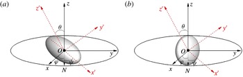
Schematic diagram of the combination of coordinate transformation from
 $(x,y,z)$
to (
 $x^{\prime },y^{\prime },z^{\prime }$
) with three Euler angles (
 $\unicode[STIX]{x1D711},\unicode[STIX]{x1D703},\unicode[STIX]{x1D713}$
). Line ‘ON’ represents the pitch line of the
 $(x,y)$
and (
 $x^{\prime },y^{\prime }$
) coordinate planes. Two coordinate systems are overlapping initially. First the particle rotates around the
 $z^{\prime }$
axis with a recession angle
 $\unicode[STIX]{x1D711}$
and then the particle rotates around the new
 $x^{\prime }$
axis (i.e. line ‘ON’) with a nutation angle
 $\unicode[STIX]{x1D703}$
. Finally the particle rotates around the new
 $z^{\prime }$
axis with an angle of rotation
 $\unicode[STIX]{x1D713}$
.

2.2 Solid particle dynamics and fluid–solid boundary interaction
In our simulation, the ellipsoidal particle is described by
 $$\begin{eqnarray}\frac{x^{\prime 2}}{a^{2}}+\frac{y^{\prime 2}}{b^{2}}+\frac{z^{\prime ^{2}}}{c^{2}}=1,\end{eqnarray}$$
where
 $a$
,
 $b$
and
 $c$
are the lengths of the three semi-principal axes of the particle in the
 $x^{\prime }$
,
 $y^{\prime }$
and
 $z^{\prime }$
axis of a body-fixed coordinate system, respectively (see figure 1). The aspect ratio of the ellipsoidal particle is defined as
 $a/b$
. The body-fixed coordinate system can be obtained by a combination of coordinate transformation around the
 $z^{\prime }-x^{\prime }-z^{\prime }$
axis with Euler angles (
 $\unicode[STIX]{x1D711},\unicode[STIX]{x1D703},\unicode[STIX]{x1D713}$
) from the space-fixed coordinate system
 $(x,y,z)$
which initially overlaps the body-fixed coordinate system. The combination of coordinate transformation is illustrated in figure 1. The evolution axis always overlaps the
 $x^{\prime }$
direction. The migration and rotation of the particle are determined by the Newton equation and Euler equation, respectively,
 $$\begin{eqnarray}\displaystyle & \displaystyle m\frac{\text{d}\boldsymbol{U}(t)}{\text{d}t}=\boldsymbol{F}(t), & \displaystyle\end{eqnarray}$$
 $$\begin{eqnarray}\displaystyle & \displaystyle \unicode[STIX]{x1D644}\boldsymbol{\cdot }\frac{\text{d}\unicode[STIX]{x1D6FA}(t)}{\text{d}t}+\unicode[STIX]{x1D6FA}(t)\times [\unicode[STIX]{x1D644}\boldsymbol{\cdot }\unicode[STIX]{x1D6FA}(t)]=\boldsymbol{T}(t), & \displaystyle\end{eqnarray}$$
where
 $\unicode[STIX]{x1D644}$
is the inertial tensor, and
 $\unicode[STIX]{x1D6FA}(t)$
and
 $\boldsymbol{T}(t)$
represent the angular velocity and the torque exerted on the particle in the body-fixed coordinate system, respectively. In the frame,
 $\unicode[STIX]{x1D644}$
is diagonal and the principal moments of inertia can be written as
 $$\begin{eqnarray}I_{x^{\prime }x^{\prime }}=m\frac{b^{2}+c^{2}}{5},\quad I_{y^{\prime }y^{\prime }}=m\frac{c^{2}+a^{2}}{5},\quad I_{z^{\prime }z^{\prime }}=m\frac{a^{2}+b^{2}}{5},\end{eqnarray}$$
where
 $m=4/3\unicode[STIX]{x1D70C}_{p}\unicode[STIX]{x03C0}abc$
is the mass of the particle and
 $\unicode[STIX]{x1D70C}_{p}$
is the density of the particle. It is not appropriate to solve (2.7) directly due to an inherent singularity (Qi Reference Qi1999). Thus four quaternion parameters are used as generalized coordinates to solve the corresponding system of equations (Qi & Luo Reference Qi and Luo2003). A coordinate transformation matrix with four quaternion parameters (Qi & Luo Reference Qi and Luo2003) is applied to transform corresponding items from the space-fixed coordinate system to the body-fixed coordinate system. With four quaternion parameters, equation (2.7) can be solved using a fourth-order-accurate Runge–Kutta integration procedure (Huang et al.
Reference Huang, Yang, Krafczyk and Lu2012b
).
In the simulations, the fluid–solid boundary interaction is based on the schemes of Aidun et al. (Reference Aidun, Lu and Ding1998) and Lallemand & Luo (Reference Lallemand and Luo2003). The accurate moving-boundary treatment proposed by Lallemand & Luo (Reference Lallemand and Luo2003) is applied to solve the problem caused by the moving curved-wall boundary condition of the ellipsoid.
The general schemes for calculation of interactive force between fluids and particles in the LBM include stress integration, momentum exchange and volume fraction models, which has been summarized and analysed by Chen et al. (Reference Chen, Cai, Xia, Wang and Chen2013). The stress integration scheme may be good but it is not so efficient (Chen et al. Reference Chen, Cai, Xia, Wang and Chen2013). Here the momentum exchange scheme is used to calculate the force exerted on the solid boundary, which is accurate and efficient (Chen et al. Reference Chen, Cai, Xia, Wang and Chen2013). The forces due to the fluid nodes covered by the solid nodes and the solid nodes covered by the fluid nodes (Aidun et al. Reference Aidun, Lu and Ding1998) are also considered in the study.
To prevent overlap of the particle and the wall, usually the repulsive force between the wall and particle should be applied (Huang et al. Reference Huang, Yang and Lu2014). Here the lubrication force model is identical to that we used in Huang et al. (Reference Huang, Yang and Lu2014) and the validation of the force model has been tested extensively by Huang et al. (Reference Huang, Yang and Lu2014).
Our previous study on the tumbling mode of an ellipsoidal particle suspended in shear flow partially validated our three-dimensional LBM code (Huang, Wu & Lu Reference Huang, Wu and Lu2012a ) because the rotational period or orbit is very consistent with Jeffery’s analytical solution (Jeffery Reference Jeffery1922). The LBM code has also been validated by Yang, Huang & Lu (Reference Yang, Huang and Lu2015) for the case of migration of a neutrally buoyant sphere in a tube Poiseuille flow. The lift force, angular and migration velocities agree well with those in Yang et al. (Reference Yang, Wang, Joseph, Hu, Pan and Glowinski2005). Here three more cases are simulated to validate our LBM code. The first one concerns migrations of a neutrally buoyant sphere in tube Poiseuille flows (Karnis et al. Reference Karnis, Goldsmith and Mason1966). The second deals with an ellipsoid particle sedimentation in a vertical circular tube under gravity. The third one describes the rotation of a prolate spheroid in shear flow. The result is shown in appendix A. The accuracy of the LBM is also investigated in § 3.1.
3 Flow problem
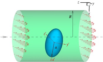
The motion of a neutrally buoyant ellipsoid inside tube flow is illustrated in figure 2, where
 $D=2R$
denotes the diameter of the circular tube. In the problem, two kinds of ellipsoids – prolate and oblate particles – are considered. Particle sizes
 $a=2b=2c$
for the prolate particle and
 $a=b/2=c/2$
for the oblate particle are considered. The
 $x^{\prime }$
axis is the evolution axis and it overlaps the major axis of the prolate particle and the minor axis of the oblate particle. To describe the orientation of the particle,
 $\unicode[STIX]{x1D6FC}$
,
 $\unicode[STIX]{x1D6FD}$
, and
 $\unicode[STIX]{x1D6FE}$
are used to denote the angles between the
 $x^{\prime }$
-axis and the space-fixed coordinates
 $x$
-,
 $y$
-, and
 $z$
-axes, respectively (
 $\cos ^{2}\unicode[STIX]{x1D6FC}+\cos ^{2}\unicode[STIX]{x1D6FD}+\cos ^{2}\unicode[STIX]{x1D6FE}=1$
).
The Reynolds number (
 $Re$
) is defined as
 $$\begin{eqnarray}Re=\frac{AU_{m}}{\unicode[STIX]{x1D708}},\end{eqnarray}$$
where
 $U_{m}$
is the central velocity of the flow without the particle and
 $A$
is the length of the major axis. For the prolate and oblate ellipsoid
 $A=2a$
and
 $A=2b$
, respectively. The confinement ratio is
 $D/A$
. It is noted that there is no gravity in this flow problem.
For all cases in our study, the fluid density is
 $\unicode[STIX]{x1D70C}_{f}=1mu/lu^{3}$
and the length of the tube is
 $L=8D$
for
 $Re<200$
, For higher-
 $Re$
cases, e.g.
 $Re>200$
, a longer computational domain, e.g.
 $L=12D$
, is adopted. In this way, the effects of the inlet/outlet boundary conditions are minimized. In most simulations, the major axis of the ellipsoidal particle is represented by
 $60lu$
, i.e.
 $A=60lu$
and
 $\unicode[STIX]{x1D70F}_{f}=0.6$
. For example, in the case of
 $D/A=1.2$
, the total mesh is approximately
 $76lu\times 76lu\times 608lu$
. The grid independence study and time-step independence study have been performed in § 3.1 and it is shown that the mesh size and the time step are sufficient to obtain accurate results.
Schematic diagram of a prolate ellipsoid in Poiseuille flow. The Poiseuille flow is in the
 $-z$
-direction.

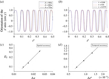
Grid independence and time-step independence studies for a prolate ellipsoid case with
 $Re=162$
,
 $D/A=2$
,
 $\unicode[STIX]{x1D70C}_{p}/\unicode[STIX]{x1D70C}_{f}=1$
, and tube length
 $L=8D$
. The initial orientation is
 $(45^{\circ },90^{\circ },45^{\circ })$
, and the initial position
 $(x_{0},y_{0})=(0,0.5)$
.
3.1 Accuracy of the LBM
The accuracy of the LBM is investigated here. Grid independence and time-step independence studies are performed. As an example, cases of a prolate ellipsoid with
 $Re=162$
and
 $D/A=2$
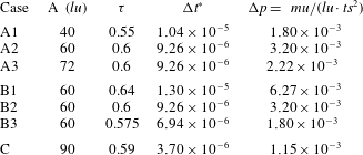
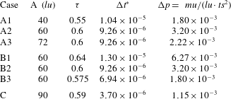
were simulated. The key parameters for the cases are shown in table 1, where
 $\unicode[STIX]{x0394}t^{\ast }$
is a normalized time and
 $\unicode[STIX]{x0394}p$
is the pressure difference between the two ends of the tube. The corresponding results for grid independence and time-step independence are shown in figure 3. In figure 3(a), the grid size is labelled, e.g. the legend ‘
 $A=40lu$
’ means 40 grids are used to discretize the particle’s major axis. From figure 3(a), it is seen that the result of
 $A=60lu$
is very close to that of
 $A=72lu$
. However, for the coarse mesh, i.e.
 $A=40lu$
, the period of the rotation has a significant discrepancy with respect to that of
 $A=72lu$
. The grid size with
 $A=60lu$
seems small enough to obtain an accurate result. Hence, for cases with
 $Re\approx O(100)$
, the grid size with
 $A=60lu$
is used.
For the time-step independence study, three cases with
 $\unicode[STIX]{x1D70F}=0.575,0.6,0.64$
were simulated (see table 1). The corresponding
 $\unicode[STIX]{x0394}t^{\ast }=\unicode[STIX]{x0394}t\unicode[STIX]{x1D708}/A^{2}=6.94\times 10^{-6},9.26\times 10^{-6},1.30\times 10^{-5}$
, respectively. It is seen from figure 3(b) that the curve for
 $\unicode[STIX]{x1D70F}=0.6$
is very close to that for
 $\unicode[STIX]{x1D70F}=0.575$
. Hence, the time step with
 $\unicode[STIX]{x1D70F}=0.6$
is small enough to get accurate results.


To test the accuracy of the present numerical method, the case with the finest mesh
 $A=90lu$
and the smallest time step
 $\unicode[STIX]{x0394}t^{\ast }=3.70\times 10^{-6}$
(Case C) is also simulated. The result is referred to as the accurate result. The
 $\cos \unicode[STIX]{x1D6FE}$
of Case A3 is very close to that of Case C. Since the error can vary with time, a time average over one period is required. After the tumbling state of the ellipsoid reaches a stable periodic state at
 $t_{1}$
with a period of
 $T$
, the relative error is defined as
 $$\begin{eqnarray}E_{2}=\frac{\displaystyle \sqrt{\int _{t_{1}}^{t_{1}+T}[\cos \unicode[STIX]{x1D6FE}(t)-\cos \unicode[STIX]{x1D6FE}_{0}(t)]^{2}\,\text{d}t}}{\displaystyle \sqrt{\int _{t_{1}}^{t_{1}+T}[\cos \unicode[STIX]{x1D6FE}_{0}(t)]^{2}\,\text{d}t}},\end{eqnarray}$$
where
 $\cos \unicode[STIX]{x1D6FE}_{0}(t)$
is the accurate result.
The least-squares data fit in figures 3(c) and 3(d) shows that the fitted slopes are 2.06 and 1.93, respectively. Hence, the present LBM solver has an approximately second-order accuracy in both space and time. That is consistent with the conclusion on accuracy of the LBM in Mei et al. (Reference Mei, Luo and Shyy1999).
4 Motion mode of a prolate spheroid
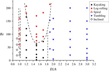
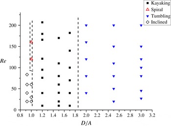
Figure 4 shows the motion mode distribution in the
 $D/A-Re$
plane for
 $\unicode[STIX]{x1D70C}_{p}/\unicode[STIX]{x1D70C}_{f}=1$
. For each point in the figure except the cases with
 $D/A\leqslant 1$
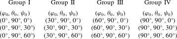
, at least eight typical cases with different initial positions and orientations were simulated. In four of the eight typical cases, we picked one initial orientation from each group listed in table 2 and the initial position is
 $(x_{0},y_{0})=(0,0)$
. In the other four cases, the initial orientation is chosen similarly, but
 $(x_{0},y_{0})=(0,0.1)$
, i.e. the particle is placed slightly away from the tube axis. It is found that the terminal rotational mode does not depend on the initial conditions.
Phase diagram for a prolate ellipsoid (
 $a/b=2$
) inside Poiseuille flow (
 $\unicode[STIX]{x1D70C}_{p}/\unicode[STIX]{x1D70C}_{f}=1$
).

Typical initial orientations.
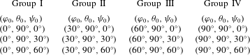
From figure 4, it is seen that the confinement of the tube plays a critical role for motion mode distribution. When
 $R<a$
, the prolate ellipsoid can only adopt the inclined mode to pass through the tube. When
 $R=a$
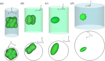
, the spiral mode as shown in figure 5(a) is identified. In the inclined mode, the
 $x^{\prime }$
-axis is inclined inside an axi-symmetric plane. When
 $R\geqslant 1.9a$
, the confinement effect is completely diminished, the particle always adopts the tumbling mode in figure 5(d), which is independent of the Reynolds number (
 $Re<200$
).
Motion modes of a prolate ellipsoid in Poiseuille flow. (a) Spiral mode, (b) kayaking mode, (c) log-rolling mode, (d) tumbling mode. The upper image is the side view and the lower image is the corresponding top view. It is noted in the Poiseuille flow the particle is not only rotating but also moving along with the flow, which is in the
 $-z$
-direction.

For
 $1.0<D/A<1.9$
, when
 $Re$
is small (e.g.
 $Re=30$
), the prolate ellipsoid adopts the kayaking mode (see figure 5
b). Suppose the
 $x^{\prime \prime }$
-axis passing through the particle centre and perpendicular to the axisymmetric plane, which passes through the tube axis and the centre of the particle. The kayaking mode adopts an intermediate orbit, where the particle performs both precession and nutation around the
 $x^{\prime \prime }$
-axis, resembling the motion of a kayak paddle (Rosén et al.
Reference Rosén, Lundell and Aidun2014).
In this confinement regime (
 $1.0<D/A<1.9$
), the fluid inertial effect is also important. When
 $Re$
is larger, the particle adopts the log-rolling mode (see figure 5
c) instead of the kayaking mode.
5 Inertial effect
5.1 Particle’s rotational energy and inertial effect of the fluid
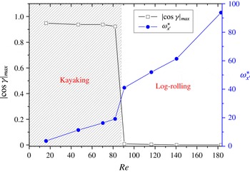
In this section we mainly discuss both inertial effects of the fluid and the particle. First, the effect of fluid inertia on the particle behaviour is discussed. Figure 6 shows
 $|\text{cos}\,\unicode[STIX]{x1D6FE}|_{max}$
as a function of
 $Re$
.
 $\unicode[STIX]{x1D6FE}$
is the angle between the
 $x^{\prime }$
-axis and the
 $z$
-direction.
 $\cos (\unicode[STIX]{x1D6FE})_{max}$
represents the maximum
 $\cos \unicode[STIX]{x1D6FE}$
in one period in the kayaking mode (see figure 5
b). It quantifies the extent of deviation from the log-rolling state. When the particle is in the log-rolling state,
 $|\text{cos}\,\unicode[STIX]{x1D6FE}|_{max}$
should be equal to zero because the major axis (
 $x^{\prime }$
-axis) is perpendicular to the
 $z$
-direction.
It is seen from figure 6 that for cases
 $D/A=1.7$
,
 $\unicode[STIX]{x1D70C}_{p}/\unicode[STIX]{x1D70C}_{f}=1$
,
 $|\text{cos}\,\unicode[STIX]{x1D6FE}|_{max}$
is not continuous as a result of the mode transition. When
 $Re$
is less than 80,
 $|\text{cos}\,\unicode[STIX]{x1D6FE}|_{max}\approx 0.9$
, the ellipsoid is in the kayaking state. As
 $Re$
increases above 90, the ellipsoid adopts the log-rolling mode. Hence, as the inertia of the fluid increases, the kayaking mode may transit to the log-rolling mode. This character can be understood as follows. When
 $Re$
increases, both the shear stress acting on the particle and the inertia of the fluid increase. The larger shear stress on the particle increases the angular velocity of the particle (
 $\unicode[STIX]{x1D714}_{x^{\prime }}$
) around the
 $x^{\prime }$
-axis (see figure 6). The energy of the rotational body is
 $(I_{x^{\prime }x^{\prime }}\unicode[STIX]{x1D714}_{x^{\prime }}^{2})/2$
. Hence the rotational energy increases. On the other hand, the larger fluid inertia may prevent the nutation or the flapping-like movement. Both the increasing rotational energy and fluid inertia are believed to assist the particle reach the log-rolling state without nutation. Although
 $\unicode[STIX]{x1D714}_{x^{\prime }}^{\ast }$
increases with
 $Re$
, the equilibrium radial position
 $r^{\ast }=r/R$
is approximately 0.46, and increases only slightly with
 $Re$
(not shown).
Transition from the kayaking mode (the shaded area) to the log-rolling mode.
 $|\text{cos}\,\unicode[STIX]{x1D6FE}|_{max}$
and normalized angular velocity
 $\unicode[STIX]{x1D714}_{x^{\prime }}^{\ast }$
as functions of
 $Re$
for
 $D/A=1.7$
,
 $\unicode[STIX]{x1D70C}_{p}/\unicode[STIX]{x1D70C}_{f}=1$
.

Phase diagram for a prolate ellipsoid (
 $a/b=4$
) inside Poiseuille flow with
 $\unicode[STIX]{x1D70C}_{p}/\unicode[STIX]{x1D70C}_{f}=1$
.

The ellipsoidal particle with aspect ratio
 $a/b=4$
is also considered in our study. The phase diagram for a prolate ellipsoid with
 $a/b=4$
inside Poiseuille flow is shown in figure 7. For
 $D/A>1.9$
, the tumbling mode still occurs. For
 $1<D/A<1.9$
, there is only the kayaking mode and the log-rolling mode is not observed. The significant difference between figures 4 and 7 lies in the log-rolling mode. The disappearance of the log-rolling mode in figure 7 may be attributed to the significantly smaller rotational energy in cases with
 $a/b=4$
. A typical example is presented below. Suppose two cases
 $D1$
and
 $D2$
have identical key parameters
 $D/A=1.5$
,
 $Re=78.4$
,
 $\unicode[STIX]{x1D70C}_{p}/\unicode[STIX]{x1D70C}_{f}=1$
,
 $a=30lu$
, and
 $\unicode[STIX]{x1D70F}=0.6$
, but in Case
 $D1$
,
 $b=c=a/2$
and in Case
 $D2$
,
 $b=c=a/4$
. That means in Cases
 $D1$
and
 $D2$
, the particle aspect ratios are 2 and 4, respectively. It is seen from figures 4 and 7 that the particles in Cases
 $D1$
and
 $D2$
adopt the log-rolling and kayaking modes, respectively. The behaviour may be understood as follows. In Case
 $D2$
the particle is more rod-like and the principal moment of inertia
 $I_{x^{\prime }x^{\prime }}$
in Case
 $D2$
is only
 $1/16$
of that in Case
 $D1$
because
 $I_{x^{\prime }x^{\prime }}=m((b^{2}+c^{2})/5)=4/3\unicode[STIX]{x1D70C}_{p}\unicode[STIX]{x03C0}abc((b^{2}+c^{2})/5)$
. In the equilibrium state, the normalized average angular velocities
 $\unicode[STIX]{x1D714}_{x^{\prime }}^{\ast }=(\unicode[STIX]{x1D714}_{x^{\prime }}A^{2})/\unicode[STIX]{x1D708}$
for Cases
 $D1$
and
 $D2$
are 36.5 and 22.3, respectively. It is seen that the energy of the rotational body
 $(I_{x^{\prime }x^{\prime }}\unicode[STIX]{x1D714}_{x^{\prime }}^{2})/2$
in Case
 $D2$
would be much smaller than that in Case
 $D1$
. A smaller energy of the rotational body may induce nutation motion when it rotates around the
 $x^{\prime }$
-axis and interacts with fluid. Hence, the particle in Case
 $D2$
more easily adopts the kayaking state instead of the log-rolling state. Again, we see that the increased rotational energy indeed assists the particle reaching the log-rolling state without nutation.
5.2 Inertial effect of the particle
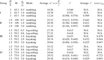
To investigate the inertial effect of the particle, twelve cases listed in table 3 were simulated. They are classified into four groups. Here
 $\unicode[STIX]{x1D70C}_{p}/\unicode[STIX]{x1D70C}_{f}$
is not limited to be unity, i.e. the cases with different
 $\unicode[STIX]{x1D70C}_{p}/\unicode[STIX]{x1D70C}_{f}$
were performed. Group I represents a wide tube case with
 $D/A=3$
. Groups III and IV denote narrow tube cases (
 $D/A=1.5$
). Group II denotes cases with
 $D/A=1.9$
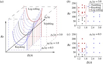
. The results of these cases with different density ratios are presented in table 3 and figure 8(b,c).
The effect of the inertia of the particle,
 $r^{\ast }=r/R$
is the equilibrium radial position.
 $|\text{cos}\,\unicode[STIX]{x1D6FE}|_{max}$
is only applicable for the kayaking mode.

In Group I, only the tumbling state is observed. The normalized tumbling rotational angular velocity increases with the density ratio
 $\unicode[STIX]{x1D70C}_{p}/\unicode[STIX]{x1D70C}_{f}$
. The particle’s lateral migration is slightly closer to the wall as
 $\unicode[STIX]{x1D70C}_{p}/\unicode[STIX]{x1D70C}_{f}$
increases. Specifically, for the case with
 $\unicode[STIX]{x1D70C}_{p}/\unicode[STIX]{x1D70C}_{f}=3.0$
, the lateral migration is periodically oscillating and
 $r^{\ast }\in (0.566,0.570)$
, i.e. the centre of mass of the ellipsoid takes a wavy trajectory in the radial direction inside an axi-symmetric plane.
Group II in table 3 shows that for the tube
 $D/A=1.9$
, again only the tumbling mode is reproduced. In the tumbling mode, the radial position of the particle’s centre of mass is continuously oscillating periodically. The magnitude of the oscillation increases with the density ratio
 $\unicode[STIX]{x1D70C}_{p}/\unicode[STIX]{x1D70C}_{f}$
. It is seen that when
 $\unicode[STIX]{x1D70C}_{p}/\unicode[STIX]{x1D70C}_{f}=0.3$
, the average
 $r^{\ast }=0.442$
with
 $r^{\ast }\in (0.412,0.470)$
, the oscillation magnitude is
 $\unicode[STIX]{x1D6FF}r=0.470-0.412=0.058$
. When
 $\unicode[STIX]{x1D70C}_{p}/\unicode[STIX]{x1D70C}_{f}=1$
and
 $\unicode[STIX]{x1D70C}_{p}/\unicode[STIX]{x1D70C}_{f}=3.0$
, it oscillates with
 $\unicode[STIX]{x1D6FF}r=0.084$
and
 $\unicode[STIX]{x1D6FF}r=0.163$
, respectively, in the radial direction. The oscillation in the radial direction is attributed to the particle’s inertia and the strong interaction between the particle and the tube wall. For a specific narrow tube, the magnitude of the radial oscillation increases with the inertia of the particle.
(a) Phase diagram in a three-dimensional parameter space. (b,c) Phase diagram in the planes
 $\unicode[STIX]{x1D70C}_{p}/\unicode[STIX]{x1D70C}_{f}=3.0$
and
 $\unicode[STIX]{x1D70C}_{p}/\unicode[STIX]{x1D70C}_{f}=0.3$
, respectively.

Phase diagram for an oblate ellipsoid inside Poiseuille flow (
 $\unicode[STIX]{x1D70C}_{p}/\unicode[STIX]{x1D70C}_{f}=1$
).

Hence, for
 $D/A\geqslant 1.9$
, the motion mode is not affected by the particle’s inertia (
 $\unicode[STIX]{x1D70C}_{p}/\unicode[STIX]{x1D70C}_{f}\leqslant 3$
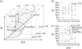
). Figure 8 shows the phase diagram in a three-dimensional parameter space. As we do not intend to provide accurate borders between the modes, it is only a schematic diagram. From figure 8, it is seen that the tumbling mode is still in the right part of the space (
 $D/A\geqslant 1.9$
), which is independent of both
 $Re$
and
 $\unicode[STIX]{x1D70C}_{p}/\unicode[STIX]{x1D70C}_{f}$
under our considered parameter space.
Groups III and IV in table 3 are the cases in narrower tubes but with lower and higher
 $Re$
, respectively. For the lower
 $Re$
cases (Group III), in the narrower tubes (
 $D/A=1.5$
) the particle adopts the log-rolling mode when
 $\unicode[STIX]{x1D70C}_{p}/\unicode[STIX]{x1D70C}_{f}=0.3$
and 0.6, while
 $\unicode[STIX]{x1D70C}_{p}/\unicode[STIX]{x1D70C}_{f}=1.0$
, 2.0 and 3.0, the state is kayaking. For higher
 $Re$
cases (Group IV), the particle adopts the log-rolling mode at
 $\unicode[STIX]{x1D70C}_{p}/\unicode[STIX]{x1D70C}_{f}=0.3$
, 0.6 and 1.0, but when
 $\unicode[STIX]{x1D70C}_{p}/\unicode[STIX]{x1D70C}_{f}=2.0$
and 3.0, it still takes the kayaking mode. Hence, for a constant
 $Re$
, the kayaking mode is preferred when the particle’s inertia increases.
Hence, for
 $D/A<1.9$
, the mode distribution would be affected by the particle’s inertia (
 $\unicode[STIX]{x1D70C}_{p}/\unicode[STIX]{x1D70C}_{f}$
). The border separating the kayaking and log-rolling modes may move upwards or downwards depending on the particle’s inertia. Figure 8 shows the approximate result. If the planes with constant
 $\unicode[STIX]{x1D70C}_{p}/\unicode[STIX]{x1D70C}_{f}$
are viewed from front to back, the border moves upwards. It means that on a plane with higher
 $\unicode[STIX]{x1D70C}_{p}/\unicode[STIX]{x1D70C}_{f}$
, the area of the kayaking mode increases. In other words, due to the inertial effect, the kayaking mode becomes more common.
6 Motion modes of an oblate ellipsoid
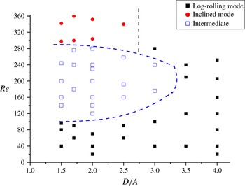
In this section, the motion modes for an oblate ellipsoid are discussed. Compared to the motion modes of the prolate ellipsoid, the phase diagram for the motion mode of the ellipsoid, i.e. figure 9, is simpler. In figure 9, only cases with
 $D>A$
are considered because the oblate ellipsoid is unable to pass through the circular tube when
 $D\leqslant A$
. For each point in the figure, similar to that in § 4, at least eight typical cases with different initial positions and orientations were simulated. It is not found that the terminal rotational mode depends on the initial conditions.
Figure 9 shows that the oblate ellipsoid always adopts the log-rolling mode in wide tubes (e.g.
 $D/A>3.2$
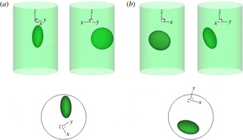
). The log-rolling mode is shown in figure 10(a). In this mode, the evolution axis of the oblate ellipsoid (the
 $x^{\prime }$
-axis) is almost perpendicular to the plane passing through the particle’s centre of mass and the tube axis. Due to the shear stress applied to the particle, it will rotate and finally reach this equilibrium state.
It is also noted that when the tube is narrow, e.g.
 $D/A<2$
, the wall effect is also strong and
 $Re$
is higher, the particle will not only adopt the log-rolling rotational mode but also perform the circumferential movement simultaneously, i.e. swirling around the tube axis due to the azimuthal instability.
Motion modes of an oblate ellipsoid in Poiseuille flow. (a) Log-rolling mode, (b) inclined mode. The upper images are two side views for each mode and the lower images are the corresponding top views. It is noted in the Poiseuille flow the particle is not only rotating but also moving along the flow. The Poiseuille flow is in the
 $-z$
-direction.

From figure 9, it is seen that inside a narrower tube, three modes may appear, which depend on
 $Re$
. The three modes are the log-rolling mode, the intermediate mode, and the inclined mode. The inclined mode is shown in figure 10(b). In this mode, the evolution axis of the oblate ellipsoid is inside instead of perpendicular to the plane passing through the particle’s centre of mass and the tube axis. Moreover, the evolution axis is no longer perpendicular to the
 $z$
-axis (see figure 10
b). Hence it is called the inclined mode. In this mode, the ellipsoid moves solely with the Poiseuille flow in the
 $-z$
-direction without rotating. We will discuss why the inclined mode exists in detail in § 6.2.
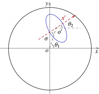
Angle between the
 $x^{\prime }$
-axis and the axi-symmetric plane passing through the tube axis and the centre of the particle.

The intermediate mode is a state between the log-rolling mode and the inclined mode. Figure 11 shows the projection of the particle in the
 $(x,y)$
-plane.
 $\unicode[STIX]{x1D70E}$
denotes the angle between the
 $x^{\prime }$
-axis and the plane passing through the tube axis and the centre of the particle. The angle
 $\unicode[STIX]{x1D703}_{1}$
can be computed from the instantaneous
 $(x,y)$
position of the particle, and it is noted that
 $\unicode[STIX]{x1D70E}=\unicode[STIX]{x1D703}_{1}-\unicode[STIX]{x1D703}_{2}$
.
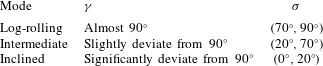
In the intermediate mode, the angle
 $\unicode[STIX]{x1D70E}$
is neither close to
 $0^{\circ }$
(the inclined mode) nor close to
 $90^{\circ }$
(the log-rolling mode). The mode combines the characteristics of both the log-rolling and inclined modes. In implementation, only the states with
 $\unicode[STIX]{x1D70E}\in (20^{\circ },70^{\circ })$
are classified to the intermediate mode, i.e. the threshold is
 $20^{\circ }$
. When
 $\unicode[STIX]{x1D70E}\in (70^{\circ },90^{\circ })$
, the mode is very close to the log-rolling mode and is classified to the log-rolling mode. When
 $\unicode[STIX]{x1D70E}\in (0^{\circ },20^{\circ })$
, the mode is classified to the inclined mode. In the intermediate mode, the oblate particle is not only inclined, i.e.
 $\unicode[STIX]{x1D6FE}$
is not close to
 $90^{\circ }$
, but also rotates around its
 $x^{\prime }$
-axis. Meanwhile, the particle is swirling around the tube axis. The characteristics of the modes are summarized in table 4.
The characteristics of the log-rolling, intermediate, and inclined modes for the oblate ellipsoid.

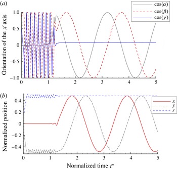
In the intermediate mode, the orientation of the
 $x^{\prime }$
-axis and trajectory position as functions of time (the case of
 $D/A=2$
,
 $\unicode[STIX]{x1D70C}_{p}/\unicode[STIX]{x1D70C}_{f}=1$
,
 $Re=100$
), where time
 $t^{\ast }$
is normalized by
 $t^{\ast }=t\unicode[STIX]{x1D708}/A^{2}$
and position is normalized by
 $D/2$
.

We would like to discuss the intermediate mode in detail. Here we take the cases of
 $D/A=2$
as an example. In the case for
 $Re=100$
,
 $\unicode[STIX]{x1D70F}=0.65$
,
 $A=80lu$
, the orientation of the
 $x^{\prime }$
-axis and trajectory position as functions of time are shown in figure 12. Initially, the particle is tumbling along a major axis due to the initial orientation
 $(\unicode[STIX]{x1D711},\unicode[STIX]{x1D703},\unicode[STIX]{x1D713})=(90^{\circ },90^{\circ },30^{\circ })$
and the initial position
 $(x_{0},y_{0})=(0,-0.19)$
. After
 $t^{\ast }>1.25$
, the oblate ellipsoid enters the intermediate mode. From figure 12, it is seen that in the intermediate mode,
 $\cos (\unicode[STIX]{x1D6FE})$
becomes constant with
 $\cos (\unicode[STIX]{x1D6FE})\approx 0.08$
(
 $\unicode[STIX]{x1D6FE}\approx 85^{\circ }$
). Also
 $\cos (\unicode[STIX]{x1D6FC})$
and
 $\cos (\unicode[STIX]{x1D6FD})$
change sinusoidally, but the angle
 $\unicode[STIX]{x1D70E}$
is a constant
 $\unicode[STIX]{x1D70E}\approx 63.9^{\circ }$
. For the swirling movement, figure 12(b) shows
 $r=\sqrt{x^{2}+y^{2}}$
is a constant, which means that the projection of the trajectory of the particle’s centre in the
 $(x,y)$
-plane is a circle.
The angle (a) and normalized angular velocity
 $\unicode[STIX]{x1D714}_{x^{\prime }}^{\ast }=\unicode[STIX]{x1D714}_{x^{\prime }}A^{2}/\unicode[STIX]{x1D708}$
(b) as functions of
 $Re$
. The red circles represent the cases at the intermediate mode (
 $D/A=2$
,
 $\unicode[STIX]{x1D70C}_{p}/\unicode[STIX]{x1D70C}_{f}=1$
).

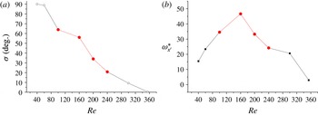
In the intermediate mode, it is found that the angle
 $\unicode[STIX]{x1D70E}$
depends on
 $Re$
. The angle
 $\unicode[STIX]{x1D70E}$
as a function of
 $Re$
is shown in figure 13(a). It is noted that only the red circles in figure 13 are classified as the intermediate mode. When
 $Re$
is lower, e.g.
 $Re\approx 40$
, the oblate ellipsoid adopts the log-rolling mode (
 $\unicode[STIX]{x1D70E}=90^{\circ }$
). The angle
 $\unicode[STIX]{x1D70E}$
decreases with
 $Re$
in the intermediate section. Hence, as
 $Re$
increases, the particle gradually changes from the log-rolling mode to the inclined mode.
Figure 13(b) shows the normalized angular velocity
 $\unicode[STIX]{x1D714}_{x^{\prime }}^{\ast }$
as a function of
 $Re$
. When
 $Re\in (40,160)$
,
 $\unicode[STIX]{x1D714}_{x^{\prime }}^{\ast }$
increases with
 $Re$
due to the increasing shear stress. However, when
 $Re>160$
, the angular velocity decreases with
 $Re$
because
 $\unicode[STIX]{x1D70E}$
decreases and the
 $(y^{\prime }-z^{\prime })$
-plane deviates significantly from the tube’s axi-symmetric plane containing
 $oo^{\prime }$
(see figure 11). The shear stress acting on the particle decreases with
 $\unicode[STIX]{x1D70E}$
decreasing, which leads to smaller
 $\unicode[STIX]{x1D714}_{x^{\prime }}^{\ast }$
.
6.1 The particle inertial effect
The approximate phase diagram in a three-dimensional parameter space for an oblate ellipsoid is shown in figure 14. The parabolic cylinder consists of a cluster of parabolic curves. Inside the parabolic cylinder there is the intermediate mode. It is seen that the mode distribution would be affected by the particle’s inertia (
 $\unicode[STIX]{x1D70C}_{p}$
). For wider tubes, the log-rolling mode is dominant in the phase diagram. For narrower tubes, the border separating the intermediate and the other two modes may move upwards or downwards depending on the particle’s inertia. If the planes with constant
 $\unicode[STIX]{x1D70C}_{p}/\unicode[STIX]{x1D70C}_{f}$
are viewed from front to back, the border moves upwards. It means that on a plane with higher
 $\unicode[STIX]{x1D70C}_{p}/\unicode[STIX]{x1D70C}_{f}$
, the area of the log-rolling mode increases. For
 $\unicode[STIX]{x1D70C}_{p}/\unicode[STIX]{x1D70C}_{f}=3$
, the inclined mode almost disappears under our considered parameter space and the log-rolling mode occupies a greater area in the
 $D/A-Re$
plane. In other words, at a slightly higher
 $Re$
, the inertia of the oblate particle helps it maintain the log-rolling state.
Phase diagram for an oblate ellipsoid. (a) Phase diagram in a three-dimensional parameter space. The vertical plane ABCD separates the inclined and log-rolling modes. The rotational mode appears inside the parabolic cylinder is the intermediate mode. The region of the inclined mode is bounded by the plane ABCD, the curved plane BCEF, and the ‘wall’ of the box. (b,c) Phase diagram in the planes
 $\unicode[STIX]{x1D70C}_{p}/\unicode[STIX]{x1D70C}_{f}=3.0$
and
 $\unicode[STIX]{x1D70C}_{p}/\unicode[STIX]{x1D70C}_{f}=0.3$
, respectively.

6.2 The inclined mode
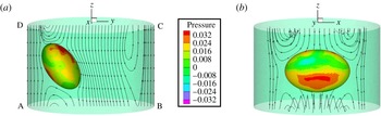
In the following, the reasons for the existence of the inclined mode are further discussed. The streamlines around the particle and pressure contours on an oblate ellipsoid are illustrated in figure 15. The pressure is normalized by
 $p=(p-c_{s}^{2}\unicode[STIX]{x1D70C}_{f})/\unicode[STIX]{x1D70C}_{f}U_{m}^{2}$
. In the case for
 $D/A=2$
and
 $Re=354$
, the dimensional parameters are
 $\unicode[STIX]{x1D70F}=0.565$
, tube length
 $L=1920lu$
and diameter
 $D=160lu$
. The oblate ellipsoid has dimensions
 $a=20lu$
,
 $b=c=40lu$
. Under the pressure difference
 $\unicode[STIX]{x0394}p=2.49\times 10^{-3}~mu/(lu\cdot ts^{2})$
between the two ends of the tube, the maximum velocity in the Poiseuille flow is
 $U_{m}=0.0958lu/ts$
and terminally the particle reaches the inclined mode with a constant velocity
 $U_{p}=-0.0559lu/ts$
in the
 $z$
-direction without rotation.
Streamlines and pressure contours on the surface of an oblate ellipsoid in Poiseuille flow. The case is
 $D/A=2$
,
 $\unicode[STIX]{x1D70C}_{p}/\unicode[STIX]{x1D70C}_{f}=1$
, and
 $Re=354$
. The position of the centre of the particle is at
 $x=0$
and
 $y=0.468$
. The streamlines are drawn in the inertial frame moving with
 $U_{p}$
, which is the particle’s velocity in the
 $z$
-direction in the space-fixed coordinate system.

Figure 15(a) shows the streamlines inside the axi-symmetric plane (plane ABCD, i.e.
 $(x=0)$
-plane) where the
 $x^{\prime }$
-axis stays. The angle between the
 $x^{\prime }$
-axis and
 $z$
-axis is approximately
 $67^{\circ }$
because
 $\cos (\unicode[STIX]{x1D6FE})\approx 0.38$
. The streamlines are drawn in an inertial frame moving with the same velocity as that of the particle. Figure 15(b) shows the pressure contours and surrounding streamlines viewed from the
 $y$
-direction. It is seen that the contours and streamlines are almost symmetric about the
 $(x=0)$
-plane.
We can qualitatively understand why the particle is able to maintain the steady state. In figure 15(a), on the lower and upper surface of the particle, the particle experienced lower and higher pressure, respectively. That may generate a positive torque (counter-clockwise). On the other hand, from the directions of the streamlines, it is seen that on the whole the shear stress acting on the surface would generate a negative torque (clockwise). Hence the torque due to the pressure difference will be balanced by the negative torque due to the viscous force acting on the surface. In this way, the inclined mode is able to be an equilibrium state.
Because both the log-rolling mode and the inclined mode are stable modes, an intermediate state combining the characteristics of both these stable modes should also possibly exist.
7 Conclusion
In this study, the behaviours of suspended particles in tube Poiseuille flow are numerically investigated. The effects of tube diameter, the inertia of both the particle and the flow, and the particle geometry (both prolate and oblate ellipsoids) are analysed. For prolate ellipsoids, aspect ratios
 $a/b=2$
and 4 are considered, while for the oblate ellipsoid, the aspect ratio is fixed to
 $1/2$
.
When a prolate particle with
 $a/b=2$
is inside a wider tube (e.g.
 $D/A>1.9$
), the terminal stable state is tumbling. When
 $1.0<D/A<1.9$
, i.e. a prolate particle is inside a narrower tube, the log-rolling or kayaking modes can appear. Which mode the particle adopts depends on the competition between the inertia of the fluid and the particle. When the inertia of the fluid is dominant, the log-rolling appears; otherwise, the kayaking mode appears. It is also found that the inclined and spiral modes may appear when
 $D/A<1$
and
 $D/A=1$
, respectively. For a prolate ellipsoid with
 $a/b=4$
, if
 $1<D/A<1.9$
, only the kayaking mode is seen, and the log-rolling mode is not observed. A possible reason is that the rotational energy in cases with
 $a/b=4$
is much smaller than that in cases with
 $a/b=2$
.
When an oblate particle is inside a wider tube (e.g.
 $D/A>3.5$
), it may adopt the log-rolling mode. It is the first time in the literature that the inclined and intermediate modes have been identified for oblate ellipsoids in narrower tubes (
 $1<D/A<3.5$
). As the inertia of the fluid increases, the oblate ellipsoid may change from the log-rolling mode to the intermediate mode, and then the inclined mode without rotation. The phase diagram of the modes is also provided.
Basically, for wider tubes, our observation is consistent with those in the literature, i.e. the prolate and oblate ellipsoids adopt tumbling and log-rolling modes, respectively (Karnis et al. Reference Karnis, Goldsmith and Mason1966; Sugihara-Seki Reference Sugihara-Seki1996; Pan et al. Reference Pan, Chang and Glowinski2008; Byeon et al. Reference Byeon, Seo and Lee2015). On the other hand, our finding is slightly different from that of Pan et al. (Reference Pan, Chang and Glowinski2008). They claimed that the final state may depend on the initial position and orientation. Here, based on limited observation, it is found that the final state does not depend on the initial states. The difference is attributed to the very short computational domain in the flow direction and the periodic inlet/outlet boundary condition in their simulations (Pan et al. Reference Pan, Chang and Glowinski2008) instead of sufficient long tubes with pressure boundary conditions.
Acknowledgements
X.Y.L. is supported by National Natural Science Foundation of China (NSFC) grant no. 11621202. H.H. is supported by NSFC:11172297 and the Fundamental Research Funds for the Central Universities.
Appendix A. Validation
A.1 Migration of a sphere in Poiseuille flows
To validate our LBM code, the migrations of a neutrally buoyant sphere in tube Poiseuille flows were studied. As we know, many extensive experiments concerning the migration of spheres in Poiseuille flows have been carried out (Karnis, Goldsmith & Mason Reference Karnis, Goldsmith and Mason1963; Karnis et al. Reference Karnis, Goldsmith and Mason1966). Here, our LBM results are compared with those obtained in experiments (Karnis et al. Reference Karnis, Goldsmith and Mason1966).
In the simulations,
 $z$
-axis denotes the tube axis. The radii of the tube and the sphere are
 $R=0.2~\text{cm}$
and
 $r=0.061~\text{cm}$
, respectively. The sphere is initially placed in the
 $(y,z)$
-plane.
 $y=0$
and
 $y/R=1$
represent the tube axis and the wall, respectively. Two cases with initial positions
 $y/R=0.21$
and 0.68 were simulated. The density of the fluid is
 $1.05~\text{g}~\text{cm}^{-3}$
and
 $\unicode[STIX]{x1D707}=\unicode[STIX]{x1D70C}\unicode[STIX]{x1D708}=1.2~\text{g}~\text{cm}^{-1}~\text{s}^{-1}$
. The flow rate is
 $Q=7.11\times 10^{-2}~\text{cm}^{3}~\text{s}^{-1}$
. Because
 $Q=(\unicode[STIX]{x03C0}R^{2}/2)U_{m}$
, the corresponding
 $Re=(U_{m}R)/\unicode[STIX]{x1D708}=0.198$
, where
 $U_{m}$
is the maximum velocity on the axis of the tube.
Migration trajectories of a neutrally buoyant sphere in Poiseuille flows. Two cases with different initial positions were simulated and compared with experimental data (Karnis et al.
Reference Karnis, Goldsmith and Mason1966). The spheres are put in the
 $(y,z)$
-plane and released from
 $y/R=0.21$
(Case 1) and
 $y/R=0.68$
(Case 2), respectively.

To make the simulations more efficient, the multi-block strategy is also used (Huang et al.
Reference Huang, Yang and Lu2014). The fine mesh size is
 $68\times 68\times 40$
, the coarse mesh size is
 $34\times 34\times 120$
and the tube length is
 $L=240lu$
. In the fine and coarse meshes, the relaxation times are set as
 $\unicode[STIX]{x1D70F}_{f}=0.9$
,
 $\unicode[STIX]{x1D70F}_{c}=0.7$
, respectively. The radius of the tube is
 $R=29.5lu$
. To match their
 $Re$
, in our simulation
 $U_{m}=8.97\times 10^{-4}lu/ts$
and the corresponding pressure drop between the inlet and outlet is
 $\unicode[STIX]{x0394}p=1.32\times 10^{-4}mu/lu/ts^{2}$
. In the simulations
 $1lu=0.00678~\text{cm}$
,
 $1ts=5.36244\times 10^{-6}~\text{s}$
,
 $1mu=3.272\times 10^{-7}~\text{g}$
.
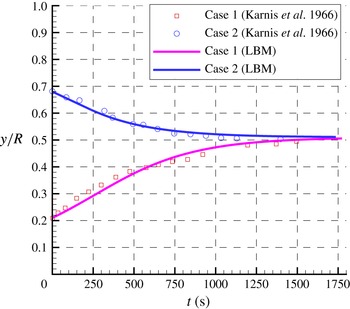
The trajectories of spheres released from the
 $y/R=0.21$
(Case 1) and
 $y/R=0.68$
(Case 2) and those measured in Karnis et al. (Reference Karnis, Goldsmith and Mason1966) are illustrated in figure 16. It is shown that the LBM results are in excellent agreement with the experimental ones. The approach to an equilibrium position roughly midway between the centre and the wall is the well-known Segre–Silberberg effect.
A.2 Sedimentation of an ellipsoid
In this section, ellipsoid sedimentation in a circular tube is simulated and compared with the cases in Swaminathan, Mukundakrishnan & Hu (Reference Swaminathan, Mukundakrishnan and Hu2006). In the simulations, the density of the fluid is
 $1.0~\text{g}~\text{cm}^{-3}$
. The gravitational acceleration is
 $g=980~\text{cm}~\text{s}^{-2}$
, the viscosity of the fluid
 $\unicode[STIX]{x1D708}=0.01~\text{cm}~\text{s}^{-1}$
, tube diameter
 $D=0.4~\text{cm}$
. In our LBM simulation,
 $(\unicode[STIX]{x1D70C}_{p}-\unicode[STIX]{x1D70C}_{f})/\unicode[STIX]{x1D70C}_{f}=\unicode[STIX]{x0394}\unicode[STIX]{x1D70C}/\unicode[STIX]{x1D70C}_{f}=0.01$
, and the length of the major axis of the ellipsoid
 $A=2a=0.1~\text{cm}$
is represented by
 $52lu$
, which means
 $1lu=0.001923~\text{cm}$
. The density of the fluid is set to be
 $\unicode[STIX]{x1D70C}_{f}=1mu/lu^{3}$
and
 $1mu=7.112\times 10^{-9}~\text{g}$
. In this particular case
 $\unicode[STIX]{x1D70F}_{f}=1.2$
. Hence,
 $1ts$
represents
 $8.63\times 10^{-5}~\text{s}$
.
The initial orientation of the particle is
 $(\unicode[STIX]{x1D719}_{0},\unicode[STIX]{x1D703}_{0},\unicode[STIX]{x1D713}_{0})=(90^{\circ },90^{\circ },45^{\circ })$
, which means the evolution axis is in the
 $(y,z)$
-plane and the angle between the
 $x^{\prime }$
axis and the
 $x$
axis is
 $45^{\circ }$
. The mesh size is
 $216lu\times 216lu\times 1800lu$
and the length of the tube is
 $L\approx 9D$
. The particle is kept in the centre of the domain using the dynamic multi-block strategy.
Trajectory of the centre of ellipsoids when they sediment in a circular tube at various Reynolds number. The centres of the ellipsoids are initially put in the axis of the tube, with the
 $x^{\prime }$
-axis inside the
 $(y,z)$
-plane. The initial orientations are
 $\unicode[STIX]{x1D6FE}=45^{\circ }$
.
 $y^{\ast }$
,
 $z^{\ast }$
are the normalized positions in the
 $y$
-axis and the
 $-z$
-direction (normalized by
 $D/2$
).

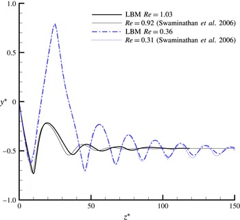
The results for comparison are shown in figure 17.
 $y^{\ast }$
and
 $z^{\ast }$
are the normalized positions on
 $y$
-axis and the
 $-z$
-direction (normalized by
 $D/2$
). It is noted that the Galileo number
 $Ga=\sqrt{(\unicode[STIX]{x0394}\unicode[STIX]{x1D70C}/\unicode[STIX]{x1D70C}_{f})(ga^{3}/\unicode[STIX]{x1D708}^{2})}$
instead of
 $Re$
is a true control parameter of the flow. However,
 $Ga$
is not given in Swaminathan et al. (Reference Swaminathan, Mukundakrishnan and Hu2006). For comparison purposes, we have to try different values of
 $\unicode[STIX]{x0394}\unicode[STIX]{x1D70C}/\unicode[STIX]{x1D70C}_{f}$
to make the simulated
 $Re$
close to the
 $Re$
in their cases (Swaminathan et al.
Reference Swaminathan, Mukundakrishnan and Hu2006). Here the cases of
 $Ga=3.43$
and 9.78 are simulated, which have
 $Re=0.36$
and 1.03, respectively.
For the case of
 $Re\approx 0.31$
, our result (
 $Re=0.36$
) agrees well with that in Swaminathan et al. (Reference Swaminathan, Mukundakrishnan and Hu2006). In this case, the particle moves and rotates inside the
 $(y,z)$
-plane. It is seen that at
 $z^{\ast }\approx 15$
, it moves across the axis. At
 $z^{\ast }\approx 25$
, the ellipsoid collides with the wall and then moves towards the axis of the tube. After it passes through the
 $z$
-axis again, the spheroid enters the inclined mode (settling off-axis with a constant inclination to the horizontal). The trajectory of the oscillatory movement in our simulation is highly consistent with the prediction in Swaminathan et al. (Reference Swaminathan, Mukundakrishnan and Hu2006).
In the case of
 $Re\approx 1.0$
, both trajectories (‘LBM
 $Re=1.03$
’ and ‘
 $Re=0.92$
Swaminathan et al. (Reference Swaminathan, Mukundakrishnan and Hu2006)’) oscillate for a while and finally reach an almost identical equilibrium
 $y$
-position. Our LBM simulations are consistent with the data in Swaminathan et al. (Reference Swaminathan, Mukundakrishnan and Hu2006).
A.3 Rotation of a prolate spheroid in shear flow
To further validate our simulation, the rotation of a prolate spheroid in shear flow was compared with the Jeffery’s solution (Jeffery Reference Jeffery1922) and those presented in figure 2 of Qi & Luo (Reference Qi and Luo2003).
In our simulations, the streamwise direction of the shear flow is along the
 $z$
-direction. The velocity gradient and the vorticity are oriented in the
 $y$
- and
 $x$
-directions, respectively. Two walls located at
 $y=0$
and
 $y=N_{y}$
move in opposite directions with speed
 $U$
. Periodic boundary conditions are applied in both the
 $x$
- and
 $z$
-directions. The particle Reynolds number is defined as
 $$\begin{eqnarray}Re=\frac{4Ga^{2}}{\unicode[STIX]{x1D708}},\end{eqnarray}$$
where the shear rate is defined as
 $G=2U/N_{y}$
and
 $a$
is the length of the semi-major axis.
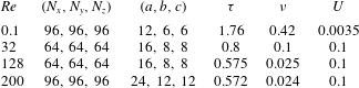
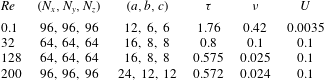
The key parameters in our simulations are listed in table 5. For the case
 $Re=32$
, 128, and 200, the parameters are identical to those in Qi & Luo (Reference Qi and Luo2003). Please refer to table 1 in their paper. Here
 $b$
and
 $c$
represent the lengths of minor axes with
 $b=c=a/2$
.
 $\unicode[STIX]{x1D70F}$
and
 $\unicode[STIX]{x1D708}$
are the relaxation times in the LBM and the kinematic viscosity, respectively.
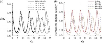
Figure 2 in Qi & Luo (Reference Qi and Luo2003) (a) is compared with our result (b). The normalized angular velocity of a prolate spheroid as a function of the dimensionless time
 $Gt$
at
 $Re=0.1$
, 32, 128, 200 and the analytic result of Jeffery’s theory at
 $Re=0$
are shown. The dimensions of both figures are the same. The simulation parameters for each case are listed in table 5.

Simulation box and particle size and key parameters for different cases.
In the simulations, the initial orientation is set as
 $(\unicode[STIX]{x1D711}_{0},\unicode[STIX]{x1D703}_{0},\unicode[STIX]{x1D713}_{0})=(90^{\circ },0^{\circ },0^{\circ })$
, which makes the particle quickly enter a tumbling mode. The tumbling rotates inside the
 $(y,z)$
-plane. Our LBM results are presented in figure 18(b). To perform the comparison, figure 2 of Qi & Luo (Reference Qi and Luo2003) is presented in figure 18(a). We note for clarity that in all the LBM results, the time and the angular velocity are normalized by
 $1/G$
and
 $G$
, respectively.
For
 $Re=0.1$
, it is seen that both our result for
 $Re=0.1$
and that of Qi & Luo (Reference Qi and Luo2003) agree very well with the Jeffery’s analytical solution. For the cases of
 $Re=32$
, 128, and 200, the rotation periods of our results are generally consistent with the corresponding periods of Qi & Luo (Reference Qi and Luo2003). The peaks of the angular velocities for the cases of
 $Re=32$
, 128, and 200 also agree well with those of Qi & Luo (Reference Qi and Luo2003), but valleys have small discrepancies; e.g. for
 $Re=200$
, the valleys are
 $0.17$
and
 $0.13$
at figure 18(a) and 18(b), respectively. The discrepancies may be attributed to the moving-boundary condition treatment. Our boundary condition scheme is based on Lallemand & Luo (Reference Lallemand and Luo2003), which is more accurate than that in Qi & Luo (Reference Qi and Luo2003).