1 Introduction
The leading-edge vortex (LEV) is an extremely common and powerful unsteady flow structure. It forms when flow separates at the leading edge of a lifting surface and the resulting shear layer rolls up into a coherent vortex near the surface of the wing. The LEV typically grows as it is fed by the shear layer and absent any mechanism for removing vorticity, eventually breaks off of the wing and convects downstream into the wake. Many forms of flight found in nature would not be possible without the LEV, but in other cases its presence can be detrimental. The LEV is found in a broad spectrum of scenarios, including a wind turbine struck by a gust or a change in wind direction, a helicopter or quad-rotor in forward flight or any kind of flapping-wing flight. The scenarios in which LEVs exist are usually very complex. In the flapping-wing context, the three-dimensional kinematics that create the lift-inducing LEV include combinations of in-plane velocity, out-of-plane velocity and pitch-rate cycles on low-aspect-ratio flexible wings (Ellington Reference Ellington1984; Wu Reference Wu2011). LEVs also form on horizontal (Hansen & Butterfield Reference Hansen and Butterfield1993) and vertical (Ferreira et al. Reference Ferreira, van Kuik, van Bussel and Scarano2008; Buchner et al. Reference Buchner, Lohry, Martinelli, Soria and Smits2015; Tsai & Colonius Reference Tsai and Colonius2016) axis wind turbines. In this context, the formation of the LEV typically occurs as part of the dynamic stall process and is a result of unsteady inflow (e.g. gusty winds or wake interactions) and/or blade motion relative to the inflow. Another common example of LEV formation is dynamic stall on a helicopter-like edgewise rotor; flow separation and vortex formation has been studied extensively in this context. Rotor blade elements encounter oscillatory changes in angle of attack, yaw angle and local flow velocity according to changes in the blade pitch, inflow, flap angle, lead/lag angle and other variables (Leishman Reference Leishman2006). In all of these cases, however, it is difficult to fully understand the physics of LEV formation in a flow where so many variables are changing simultaneously. In order to study the problem of LEV formation and convection more fundamentally, these complex flows are frequently decomposed into their constitutive components in works which present the more fundamental side of LEVs, i.e. studies of LEV formation on flat plates undergoing transient or periodic motions in surge, pitch, plunge and/or rotation (Eldredge & Jones Reference Eldredge and Jones2019).
An LEV that results from an unsteady pitch-up motion of the lifting surface is often referred to as a dynamic stall vortex (DSV). Although the current work focuses on flow separation due to surging rather than pitch-up motions, many similarities will become evident, and pitch-up dynamic stall has been studied extensively in the context of rotorcraft (McCroskey Reference McCroskey1982), wind turbines (Hansen & Butterfield Reference Hansen and Butterfield1993), as well as more fundamental flows (Eldredge & Jones Reference Eldredge and Jones2019). Due to the extremely large body of work in this area, it is not possible to provide a detailed literature review of dynamic stall here, but some examples of more recent studies making use of flow visualization (Panda & Zaman Reference Panda and Zaman1994; Choudhry et al. Reference Choudhry, Leknys, Arjomandi and Kelso2014), particle imaging velocimetry (PIV) (Ol et al. Reference Ol, Bernal, Kang and Shyy2009; Mulleners & Raffel Reference Mulleners and Raffel2012, Reference Mulleners and Raffel2013), surface pressure measurements (Gardner et al. Reference Gardner, Richter, Mai, Altmikus, Klein and Rohardt2013; Disotell et al. Reference Disotell, Nikoueeyan, Naughton and Gregory2016; Lind & Jones Reference Lind and Jones2016) and computations (Ferreira et al. Reference Ferreira, van Kuik, van Bussel and Scarano2008; Visbal Reference Visbal2011; Gharali & Johnson Reference Gharali and Johnson2013; Hodara et al. Reference Hodara, Lind, Jones and Smith2016; Tsai & Colonius Reference Tsai and Colonius2016; Kaufmann, Merz & Gardner Reference Kaufmann, Merz and Gardner2017; Visbal & Garmann Reference Visbal and Garmann2018) can be found in the references. Nearly all of this work focuses on a pitching wing in a constant free stream. However, in practice, dynamic stall often occurs in a time-varying free stream, and as the convection of vorticity into the wake is greatly dependent on the flow velocity, we expect the convection of the LEV to depend greatly on flow velocity as well. Therefore, while these studies provide much insight into the formation of the LEV, the specifics of its convection may have limited applicability to real-world kinematics.
Although dynamic stall and the ensuing LEV formation is typically attributed to a rapid increase angle of attack, this is not the only source of LEV formation. LEVs similar to the pitch-induced DSV have been observed in kinematics that have dominant unsteady changes in velocity rather than angle of attack. This can be shown to be the case for a high-advance-ratio rotor, just one example of a complex three-dimensional flow in which dynamic stall is known to occur. The advance ratio of a rotor, analogous to the tip speed ratio of a wind turbine, is the ratio of forward flight speed
 $U$
to a blade tip speed
 $\unicode[STIX]{x1D6FA}R$
, such that the advance ratio
 $\unicode[STIX]{x1D707}$
is given by
 $\unicode[STIX]{x1D707}=U/(\unicode[STIX]{x1D6FA}R)$
. The high-advance-ratio rotor is a particularly convenient comparison to the current study of surging wings in rectilinear motion in that while the flow over a rotor blade has a high degree of three-dimensionality due to blade rotation, the high aspect ratio of the blades allows for the effect of the tip vortex to be neglected. Furthermore, at high advance ratios, flow on a retreating edgewise rotor blade reverses direction such that the net flow is from the sharp geometric trailing edge to the blunt geometric leading edge. Dynamic stall thus occurs in reverse flow, and the aerofoil acts very much like a flat plate on which flow separation occurs at the sharp aerodynamic leading edge. This allows for a unique flow that bears close resemblance to the oft-studied canonical flows over a flat plate, while also introducing the complexities of a time-varying free stream, a high degree of three-dimensionality and large rotational accelerations.
As an example of LEV formation in a complex environment, consider the dynamic stall vortex observed by Lind et al. (Reference Lind, Trollinger, Manar, Chopra and Jones2017) beneath the retreating rotor blade of a high-advance-ratio rotor. Although dynamic stall is commonly attributed to pitch-up motions, it can be shown that in the reverse flow region of the rotor disc, the greater unsteadiness is the time-varying free stream. Furthermore, reconstruction of the blade pitch from Lind’s rotor tests shows that the blade pitch was decreasing throughout the entire reverse flow region. An unsteady angle of attack increase is necessary for an LEV to be created via pitch-induced dynamic stall. It is therefore proposed that this LEV was a result of the blade elements’ surge into greater reverse flow velocities (i.e. the time-varying free stream), since angle of attack increase was not present. This observation motivates an exploration of the aerodynamic properties of wings in pure surging motions. In the same way that dynamic stall experiments simplify complex kinematics into an angle of attack oscillation, pure surge experiments simplify the problem into a velocity oscillation.
Early work on wings undergoing surging motions began with unsteady potential flow models at low incidence. Because of added mass effects and the influence of the aerofoil’s wake, traditional thin aerofoil theory could not be applied in a quasi-steady manner to flows of variable velocity. Isaacs (Reference Isaacs1945) adapted thin aerofoil theory to account for these effects in fixed incidence periodic flows and solved for lift as a Fourier series. Greenberg (Reference Greenberg1947) simplified and adapted Isaacs’s theory by assuming the wake was sinusoidal, and, incorporating the work of Theodorsen (Reference Theodorsen1935), obtained closed form expressions for the lift and moment of an aerofoil in attached flow undergoing sinusoidal pitch, surge and plunge. Greenberg’s model is used as a reference for collected data in the present work.
Experimental work in unsteady surge is far less common than that with pitch oscillations. A few researchers first superimposed time-varying components of velocity with pitch oscillations to determine the effect of free-stream variability on dynamic stall (Pierce, Kunz & Malone Reference Pierce, Kunz and Malone1978; Favier et al. Reference Favier, Agnes, Barbi and Maresca1988). Maresca, Favier & Rebont (Reference Maresca, Favier and Rebont1979) conducted an extensive study of pure sinusoidal surge (without pitching) at low and high incidence with variable frequency and amplitude. At high incidence, Maresca observed vortex formation and lift characteristics similar to those traditionally expected from pitch-induced dynamic stall. Later, Gursul & Ho (Reference Gursul and Ho1992) also performed experiments on a wing in an sinusoidally varying free stream and observed high aerodynamic loads and the formation of large LEVs.
More recently, Dunne & McKeon (Reference Dunne and McKeon2015) studied a sinusoidally pitching and surging wing in recirculating water channel. These experiments were designed to mimic the blade kinematics of a vertical axis wind turbine, but in rectilinear rather than rotational motion so as to remove the effect of Coriolis forces. Using dynamic mode decomposition (DMD) on time-resolved velocity fields, they were able to identify the most significant dynamic structures (i.e. the leading-edge and trailing-edge vortices) and capture the process of dynamic stall including separation, LEV formation and reattachment with only 5 modes. The most dynamically relevant time scale in the separation and reattachment process was found to be the that of the unsteady free stream.
Granlund et al. (Reference Granlund, Monnier, Ol and Williams2014) and Granlund, Ol & Jones (Reference Granlund, Ol and Jones2016) performed experiments on sinusoidally surging wings in a water channel and an unsteady wind tunnel. Granlund et al. (Reference Granlund, Monnier, Ol and Williams2014) compared two cases: a wing moving sinusoidally fore and aft in a constant free stream, and a fixed wing in an unsteady free stream. The two were shown to be equivalent in both attached and separated flow if added mass and buoyancy effects are properly accounted for. Granlund et al. (Reference Granlund, Ol and Jones2016) focused on more aggressive wing motions in which the wing was driven at velocities large enough to result in flow reversal. Both studies found excellent agreement with Isaacs’s and Greenberg’s potential flow models throughout the velocity cycle at low wing incidence (even in reverse flow), and surprisingly good agreement at high incidence in reverse flow. During high incidence acceleration, however, large discrepancies between lift measurements and model predictions were found to arise due to the formation of the dynamic stall LEV.
Recent research on the fundamental physics of surging wings was conducted by Manar & Jones (Reference Manar and Jones2017), who extensively studied and modelled the wake of a surging flat plate at high incidence using PIV measurements and vorticity fields. For the full length of flow acceleration, Manar observed that the change in circulation flux over the wing,
 $\text{d}\unicode[STIX]{x1D6E4}/\text{d}t$
, was remarkably linear in time. The slope of
 $\text{d}\unicode[STIX]{x1D6E4}/\text{d}t$
in time (equivalently,
 $\text{d}^{2}\unicode[STIX]{x1D6E4}/\text{d}t^{2}$
) was found to be almost invariant with angle of attack as long as the flow was separated. Manar’s experiments, which were conducted at
 $Re<20\,000$
, suggest that in separated surging flows,
 $\text{d}^{2}\unicode[STIX]{x1D6E4}/\text{d}t^{2}$
is only dependent on the acceleration of the wing.
Using a similar type of analysis on the LEV found in the rotor’s reverse flow region, Lind et al. (Reference Lind, Trollinger, Manar, Chopra and Jones2017) demonstrated a linear increase of vortex strength
 $\unicode[STIX]{x1D6E4}_{v}$
with the distance travelled through the flow by the blade element. The rate of this linear increase was found to be invariant with the advance ratio. Note that because Manar’s kinematics were a linear acceleration from rest, his plots of circulation flux against time are a scaled equivalent to Lind’s plots of circulation against blade element travel. Yet, they do not show the same result: Manar’s data show a variance of
 $\text{d}^{2}\unicode[STIX]{x1D6E4}/\text{d}t^{2}$
with acceleration, while Lind’s (with different flow accelerations for different advance ratios) show invariance.
The present work is an experimental campaign to further explore the nature of surging-wing aerodynamics, with a particular focus on the LEV and its resulting forces and pressures. The aim of this work is to characterize and quantify the formation and evolution of the LEV and the resulting suction peak on a surging wing, to identify similarities and differences with respect to the more common pitch-up dynamic stall and to assess the potential for developing reduced-order models of these types of flows. Expanding on the work of Maresca et al. (Reference Maresca, Favier and Rebont1979), sinusoidal velocity profiles with a wider range of frequencies and amplitudes are explored with PIV, force and surface pressure measurements. The model discrepancies found by Granlund et al. (Reference Granlund, Ol and Jones2016) are also recreated and further explored. Special consideration is given to the convection of the LEV in each case using pressure measurements. Throughout this work, several similarities with the onset of pitching-wing dynamic stall are observed and references are made to previous work in that area for comparison. Finally, PIV data are collected for high incidence reverse flow surge experiments for comparison to the high-advance-ratio rotor tests from Lind et al. (Reference Lind, Trollinger, Manar, Chopra and Jones2017), with particular attention given to the development of LEV circulation and unsteady aerodynamic loading throughout the wing motion.
2 Experimental methods
Experiments were performed in a
 $7\times 1.5\times 1~\text{m}$
water-filled tow tank. A gantry moved over the length of the tank according to prescribed tow velocity kinematics. The gantry held a rotary motor (with rotation about the vertical axis), which housed two linear motors (that moved along the vertical axis). These vertically moving linear motors were attached to control rods that reached below the surface of the water. The test models were attached to these two control rods. The models’ speed, pitch, elevation and rotation were all prescribed through carefully defined kinematics sent to the motors.
In this case, the model was prescribed velocity kinematics at constant pitch and elevation with zero rotation. The kinematics used in this experiment are
 $$\begin{eqnarray}v(\unicode[STIX]{x1D719})=v_{0}[1+\unicode[STIX]{x1D706}\sin (\unicode[STIX]{x1D719})],\end{eqnarray}$$
where
 $v_{0}$
is the average velocity of the sinusoid (i.e. its constant offset),
 $\unicode[STIX]{x1D706}$
is the amplitude of the sinusoid expressed as a ratio to the average velocity, and the variable
 $\unicode[STIX]{x1D719}$
gives the position within the sinusoid. When compared to a rotor,
 $v_{0}$
corresponds to the blade-tangential velocity
 $U_{T}$
directly induced by the blade’s rotation,
 $\unicode[STIX]{x1D706}$
corresponds to the amplitude of oscillations that arise from forward flight and
 $\unicode[STIX]{x1D719}$
corresponds to the blade azimuth.
The effects of varying oscillation amplitude and frequency were explored in these experiments. Greenberg (Reference Greenberg1947) defined the reduced frequency
 $k$
for a surging wing as
 $$\begin{eqnarray}k=\frac{\unicode[STIX]{x1D714}_{v}c}{2v_{0}},\end{eqnarray}$$
where
 $\unicode[STIX]{x1D714}_{v}$
is the circular frequency of velocity oscillation in
 $\text{rad}~\text{s}^{-1}$
and
 $c$
is the chord length of the wing. Recognizing that
 $\unicode[STIX]{x1D719}=\unicode[STIX]{x1D714}_{v}t$
, the definition of the kinematics could also be written as
 $$\begin{eqnarray}v(t)=v_{0}\left[1+\unicode[STIX]{x1D706}\sin \left(\frac{2kv_{0}}{c}t\right)\right].\end{eqnarray}$$
The convective time is also introduced,
 $t^{\ast }=v_{0}t/c$
, so the wing kinematics used here can be written most neatly as
 $$\begin{eqnarray}v(t^{\ast })=v_{0}[1+\unicode[STIX]{x1D706}\sin (2kt^{\ast })].\end{eqnarray}$$
2.1 Full sinusoid tests
Two sets of experiments were performed with this kinematic definition. In the first set of experiments, the average velocity
 $v_{0}$
was fixed and corresponded to an average Reynolds number
 $Re_{0}$
of 40 000. The velocity sinusoids had amplitude ratios of
 $\unicode[STIX]{x1D706}=\{0.25,0.5,0.75,1.0\}$
, in combination with reduced frequencies,
 $k=\{0.16,0.217,0.309,0.511\}$
, for a total of sixteen unique kinematic cases. These kinematics were performed at a low incidence at
 $\unicode[STIX]{x1D6FC}=5^{\circ }$
and at high incidence with
 $\unicode[STIX]{x1D6FC}=25^{\circ }$
.
Sample kinematics for full sinusoid cases. (a) Sketch of wing motion in the tow tank. (b) Reynolds number as a function of time for a full run where
 $\unicode[STIX]{x1D706}=0.75$
,
 $k=0.217$
. Data collection began after
 $3/4$
of a start-up cycle was completed.

An example of the tow kinematics for a full run of these experiments is shown in figure 1. For all cases, the wing entered the velocity sinusoid at the minimum velocity point. Three quarters of a cycle after this point, data collection began. This continued for as many cycles as possible, limited by the length of the tank and dependent on the reduced frequency of the case. Data collection ended one quarter cycle before the model exited the velocity sinusoid. With the amplitude ratio
 $\unicode[STIX]{x1D706}=0.75$
, the amplitude of oscillations in this case is
 $\unicode[STIX]{x1D706}Re_{0}=30\,000$
. Every kinematic case (each combination of
 $\unicode[STIX]{x1D706}$
and
 $k$
) was performed a number of times such that there were at least 15 total data collection periods for each case. For cases with
 $k=\{0.16,0.217,0.309,0.511\}$
, there were correspondingly
 $\{1,2,3,5\}$
data collection periods per run. Notice in figure 1(b) that within a data collection period the velocity profile took the shape of a negative sine wave. A shift is therefore introduced to yield the final definition of the kinematics during data collection, given by (2.5) and (2.6).
 $$\begin{eqnarray}\displaystyle & \displaystyle v(t)=v_{0}(1-\unicode[STIX]{x1D706}\sin (\unicode[STIX]{x1D719})), & \displaystyle\end{eqnarray}$$
 $$\begin{eqnarray}\displaystyle & \displaystyle \unicode[STIX]{x1D719}=\frac{2kv_{0}}{c}t=2kt^{\ast }. & \displaystyle\end{eqnarray}$$
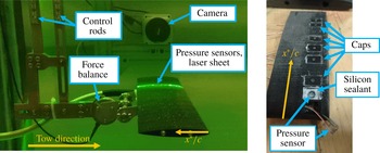
The model towed by these kinematics, shown in figure 2(a), was a NACA 0012-64 wing with a 64 cm span and a 10.47 cm chord, resulting in an aspect ratio of 5.8. For the highly unsteady motions and short times of interest here, a large region of two-dimensional flow is expected over the centre region of this relatively high-aspect-ratio model. The model was constructed from 15 separate segments aligned along two stainless steel spars to provide rigidity. One segment, which was 3D printed, housed eight pressure sensors aligned along the chord, as shown in figure 2(b). Silicon sealant was injected below the sensors and around the sensor ring to prevent leakage. A cap was then placed over the sensor to create a smooth surface. This chordwise row of sensors was 17.1 cm (1.6 chord lengths) from the left edge of the wing. The chordwise location of the sensors is given in figure 3.
Experimental set-up. (a) The model used in these experiments, installed in the water tank and shown at
 $\unicode[STIX]{x1D6FC}=0^{\circ }$
. (b) Sealed pressure sensors embedded in one segment of the model.

The placement of pressure sensors on the wing, viewed at
 $\unicode[STIX]{x1D6FC}=0^{\circ }$
. Sensors are located at
 $x^{\ast }/c=\{0.05,0.125,0.2,0.35,0.45,0.55,0.725,0.80\}$
.

The pressure sensors (MS5401-BM, produced by Intersema Sensoric) were each configured as one arm of a Wheatstone bridge with a signal sensitivity of approximately
 $2~\text{mV}~\text{kPa}^{-1}$
. Each sensor signal was run through an electrical first-order low-pass filter with a cutoff frequency of 67 Hz to reject strong high-frequency noise created by the gantry motors. The pressure signals were collected by a National Instruments USB-6341 DAQ board at a sampling rate of 1 kHz. The sensors were calibrated at the beginning of each run using the hydrostatic pressure difference associated with a commanded change in the model’s height.
The wing was mounted to a dynamically calibrated force balance, highlighted in figure 2(a). The balance is an ATI Mini 40, which saturates at 40 N of total force or a 2 N-m moment. Load measurements were collected during each test with a sampling frequency of 1 kHz.
Particle imaging velocimetry (PIV) data were also collected for a selection of cases: (
 $\unicode[STIX]{x1D706}=0.25$
,
 $k=0.16$
), (
 $\unicode[STIX]{x1D706}=0.25$
,
 $k=0.511$
), (
 $\unicode[STIX]{x1D706}=0.75$
,
 $k=0.217$
), (
 $\unicode[STIX]{x1D706}=0.75$
,
 $k=0.309$
), (
 $\unicode[STIX]{x1D706}=1.0$
,
 $k=0.16$
), (
 $\unicode[STIX]{x1D706}=1.0$
,
 $k=0.511$
). The laser optics were set such that the laser sheet was emitted from a Powell lens fixed to the gantry, and then passed through an acrylic block to allow a clean transition into the water. The laser sheet was aligned to the chord of the wing, and contacted the wing 1.3 cm inboard of the pressure sensors, or 1.8 chords from the left wing tip. The camera, which was synchronized with the firing of the laser, was attached to an arm that was also fixed to the gantry. The camera, laser, and model therefore all moved with the tow kinematics prescribed for the gantry so that the view seen by the camera was unchanged throughout each data collection period; time-resolved velocity fields were measured in a wing-fixed reference frame. The selected cases were run such that PIV was collected for at least five data collection periods for each case. These five cycles were phase averaged to obtain the data presented in § 3. Five cycles were found to be sufficient to capture the converged properties of the large-scale vortex that is of primary interest in the current work. Due to the relatively small number of cycles in the ensemble average, however, small-scale flow structures do still appear in these images although they are much less repeatable.
2.2 Reverse flow tests
In order to compare the present work on a canonical surging wing to previous work on high-advance-ratio rotors, additional experiments were performed using parameters corresponding to the experiments of Lind et al. (Reference Lind, Trollinger, Manar, Chopra and Jones2017). That rotor had a radius of
 $R=0.85~\text{m}$
, rotation speed of
 $\unicode[STIX]{x1D6FA}=30\unicode[STIX]{x03C0}~\text{rad}~\text{s}^{-1}$
and blade chord
 $c=0.08~\text{m}$
. The reverse flow vortex was observed at a non-dimensional radial location
 $\unicode[STIX]{x1D702}=0.4$
for advance ratios
 $\unicode[STIX]{x1D707}$
of
 $0.6$
,
 $0.7$
,
 $0.8$
and
 $0.9$
. For the current work, these rotor parameters were translated into pure surge experiments using only the tangential velocity component,
 $U_{T}$
, incident on the rotor blade element at 40 % radius. (In this translation, the effects of inflow, as well as rotor blade flap and lead/lag motions were neglected.) In the rotor case, the dimensional oscillation magnitude of the corresponding
 $U_{T}$
sinusoid is equal to the rotor’s free-stream velocity, and the oscillation frequency of the
 $U_{T}$
sinusoid is equal to the rotor’s rotational frequency. The average velocity is equal to the product of rotational speed and the radial location of a blade element. This translates to a reduced frequency that depends only on chord length and radial location,
 $$\begin{eqnarray}k=\frac{\unicode[STIX]{x1D714}_{v}c}{2v_{0}}=\frac{\unicode[STIX]{x1D6FA}c}{2\unicode[STIX]{x1D6FA}r}=\frac{c}{2r},\end{eqnarray}$$
and to an amplitude ratio that depends on the advance ratio of the rotor and the non-dimensional radial location of the blade element,
 $$\begin{eqnarray}\unicode[STIX]{x1D706}=\frac{U_{\infty }}{v_{0}}=\frac{U_{\infty }}{(\unicode[STIX]{x1D6FA}R)\unicode[STIX]{x1D702}}=\frac{\unicode[STIX]{x1D707}}{\unicode[STIX]{x1D702}}.\end{eqnarray}$$
While it is possible to characterize the kinematics of a rotor blade element with these parameters, it should be emphasized that by translating the rotational motion of the rotor blade into a purely rectilinear motion, three-dimensional effects including those of radial flow, vortex tilting and Coriolis forces are necessarily neglected. We therefore expect that some differences in the flow field will arise between the previously reported rotor results and the present case of interest – the surging wing.
The rotor parameters of Lind et al. (Reference Lind, Trollinger, Manar, Chopra and Jones2017) correspond to a reduced frequency of
 $k=0.117$
and a mean Reynolds number of
 $Re_{0}\approx 170\,000$
. Converting the rotor advance ratios
 $\unicode[STIX]{x1D707}=\{0.6,0.7,0.8,0.9\}$
to the canonical pure surge kinematics results in amplitude ratios of
 $\unicode[STIX]{x1D706}=\{1.50,1.75,2.00,2.25\}$
. Due to the physical limitations of the tow tank, these kinematics could not be implemented as a full sinusoid. However, because the flow situation of interest was the surge into reverse flow, the sinusoid could be trimmed to include only the reverse flow portion of the cycle as shown in figure 4. To ensure a clean entry into reverse flow, the tow kinematics entered and exited the sinusoid when it crossed
 $v=0.1~\text{m}~\text{s}^{-1}$
forward flow. In addition to this modification from the true
 $U_{T}$
profile, the Reynolds numbers achieved in wind tunnel tests could not be matched in the tow tank, so a
 $Re_{0}$
of 60 000 was used for these experiments. This was not expected to significantly change the results because flow separates from the sharp aerodynamic leading edge (in reverse flow) regardless of Reynolds number (Lind et al.
Reference Lind, Smith, Milluzzo and Jones2016). In order to match the aerofoil shape of the rotor blades in Lind et al. (Reference Lind, Trollinger, Manar, Chopra and Jones2017), the model used for this set of experiments was a NACA 0012 wing with 56 cm span and 11.4 cm chord. The wing was 3D printed and rigidity was provided by a stainless steel spar. The wing was mounted at an angle of attack of
 $\unicode[STIX]{x1D6FC}_{rev}=25^{\circ }$
.
Sample kinematics for reverse flow cases. (a) Sketch of surging-wing motion in the tow tank. (b) Reverse flow surge test kinematics, shown in relation to
 $U_{T}$
for a rotor blade element.

Only PIV data were collected for this set of experiments. The laser sheet contacted the wing 9.5 cm (0.83 chords) from the left wing tip. This position was selected so that the data collection area was sufficiently outboard to avoid any wake effects downstream of the control rods. Each run was performed five times, with one data collection period per run.
2.3 Summary
The experimental test matrix for the full sinusoid tests is summarized in table 1. In addition, reverse flow experiments were performed at a fixed reduced frequency and four amplitude ratios. Force and surface pressure measurements were phase averaged over 15 data collection cycles. PIV was phase averaged across five data collection periods.
Experimental test matrix and data collection types for full sinusoid test cases in forward flow at
 $Re_{0}=40\,000$
,
 $\unicode[STIX]{x1D6FC}=\{5^{\circ },25^{\circ }\}$
.

3 Results
The two sets of experimental results are presented below. The fundamental physics of LEV convection in surge are explored first, using results from full sinusoid tests at low and high incidence, as described in § 2.1. We begin by comparing force measurements at low and high incidence to the force prediction from Greenberg’s potential flow model.
3.1 Comparison to Greenberg’s force model
Low incidence control tests were performed to validate the experimental set-up. The wing was towed in sinusoidal free-stream oscillations at a
 $5^{\circ }$
angle of attack. Greenberg’s potential flow model for the total force on a thin aerofoil subject to simultaneous heave, pitch, and surge oscillations can be simplified to model this case. Setting the heave and pitch terms equal to zero, Greenberg’s model for the total force per unit span
 $P$
reduces to (3.1).
 $$\begin{eqnarray}P=-\frac{c}{2}\unicode[STIX]{x03C0}\unicode[STIX]{x1D70C}\unicode[STIX]{x1D6FC}\left(\frac{c}{2}\dot{v}+2vv_{0}+(2vv_{0}\unicode[STIX]{x1D706})\mathbb{R}\{C(k)\text{e}^{\text{i}\unicode[STIX]{x1D714}_{v}t}\}\right).\end{eqnarray}$$
Values for density
 $\unicode[STIX]{x1D70C}$
and chord
 $c$
are fixed for this experimental set-up and constant for all full sinusoid runs. Other constants
 $\unicode[STIX]{x1D6FC}$
,
 $\unicode[STIX]{x1D706}$
,
 $k$
and
 $v_{0}$
are parameters of the kinematics. The circular frequency of the velocity cycle,
 $\unicode[STIX]{x1D714}_{v}$
, is proportional to the reduced frequency as
 $\unicode[STIX]{x1D714}_{v}=2kv_{0}/c$
. Theodorsen’s constant
 $C(k)$
is obtained from Bessel functions. As shown by Theodorsen (Reference Theodorsen1935),
 $C(k)$
is only dependent on reduced frequency. Therefore for the test cases where
 $k=\{0.16,0.217,0.309,0.511\}$
, the values are
 $C(k)=\{0.7628-0.1876\text{i},0.7147-0.1879\text{i},0.6606-0.1781\text{i},0.5955-0.1492\text{i}\}$
, respectively. Arrays of
 $v$
,
 $\dot{v}$
and
 $t$
are obtained from the kinematics for a particular case, and a phase shift is introduced to apply the equation (which takes the shape of
 $+\cos$
) to the data collection period (which takes the shape of
 $-\text{sin}$
).
Greenberg’s model can therefore be evaluated over the data collection cycle. This potential flow solution is shown with the measured force (as well as its lift and drag decomposition) for four combinations of amplitude ratio and reduced frequency in figure 5. As shown in the figure, measurements agree well with Greenberg’s model for cases of low incidence. Most of the net force is in the lift direction and, especially at low amplitude ratios, drag is nearly negligible. The greatest lift-to-drag ratio occurs for the (
 $k=0.16$
,
 $\unicode[STIX]{x1D706}=0.75$
) case where
 $(L/D)_{max}\approx 7.5$
. The other cases produce lower lift and/or greater drag and
 $(L/D)_{max}\approx \{5.3,5.8,5.9\}$
for the (
 $k=0.16$
,
 $\unicode[STIX]{x1D706}=0.25$
), (
 $k=0.309$
,
 $\unicode[STIX]{x1D706}=0.25$
) and (
 $k=0.309$
,
 $\unicode[STIX]{x1D706}=0.75$
) cases, respectively.
Phase averaged force measurements along with Greenberg’s model at different velocity oscillation amplitude and frequency combinations at
 $\unicode[STIX]{x1D6FC}=5^{\circ }$
. The measurements are normalized by the measured force when
 $\unicode[STIX]{x1D706}=0$
. Greenberg’s model is normalized by its steady state output,
 $P=-\unicode[STIX]{x03C0}\unicode[STIX]{x1D6FC}\unicode[STIX]{x1D70C}cv_{0}^{2}$
.

Phase averaged force measurements along with Greenberg’s model at different velocity oscillation amplitude and frequency combinations at
 $\unicode[STIX]{x1D6FC}=25^{\circ }$
. The same normalizations are used as in figure 5.

At high incidence, however, Greenberg’s potential flow solution does not match experimental results well for some cases. Normalized force measurements for these same kinematics performed at
 $\unicode[STIX]{x1D6FC}=25^{\circ }$
are compared with Greenberg’s model in figure 6. While Greenberg’s model assumes an attached flow condition that is not present at this high angle of attack, the normalization allows the model to reasonably approximate the force at low frequencies and amplitudes, e.g. for
 $k=0.16$
,
 $\unicode[STIX]{x1D706}=0.25$
. However, increasing the frequency or amplitude of the velocity sinusoid results in greater disparity between the measurements and Greenberg’s model. In particular, measurements diverge from the model near
 $\unicode[STIX]{x1D719}=150^{\circ }$
and remain significantly above model predictions through the end of the cycle. As the reduced frequency and amplitude increase, Greenberg’s model increasingly under-predicts the force measurements in this region. At high reduced frequencies, the relative contribution of the non-circulatory term in Greenberg’s model becomes large (see also Theodorsen Reference Theodorsen1935), and we therefore expect large non-circulatory forces. It will also be shown that strong LEVs form at the higher reduced frequencies tested here. Greenberg’s model assumes attached flow and therefore does not account for any force contributions that may arise from LEV formation and so under-predicts the resulting force. Note that this trend may not be extrapolated to extremely high reduced frequencies beyond the current test matrix where wing motion may be too fast to allow for the development of strong LEVs.
Decomposing the total force measured on the wing into lift and drag (as shown in figure 6) highlights the large component forces that occur during unsteady motions at high incidence. Despite very large net forces, lift-to-drag ratios are lower here than at low incidence as the net force in separated flow tends to be nearly normal to the wing surface. At high incidence, the greatest lift-to-drag ratio occurs for the (
 $k=0.309$
,
 $\unicode[STIX]{x1D706}=0.75$
) case where
 $(L/D)_{max}\approx 3.2$
.
 $(L/D)_{max}\approx \{2.0,2.3,2.5\}$
for the (
 $k=0.16$
,
 $\unicode[STIX]{x1D706}=0.25$
), (
 $k=0.309$
,
 $\unicode[STIX]{x1D706}=0.25$
) and (
 $k=0.16$
,
 $\unicode[STIX]{x1D706}=0.75$
) cases, respectively.
Phase averaged pressure coefficient from each sensor at different velocity oscillation amplitude and reduced frequency combinations,
 $\unicode[STIX]{x1D6FC}=5^{\circ }$
.

It should also be noted that, at high incidence, the peak force measurement significantly leads the peak force prediction (which occurs at the maximum velocity,
 $\unicode[STIX]{x1D719}=270^{\circ }$
). This is particularly true at lower reduced frequencies. In the case of
 $k=0.16$
,
 $\unicode[STIX]{x1D706}=0.75$
, the first force peak occurs at
 $\unicode[STIX]{x1D719}=215^{\circ }$
, while at
 $k=0.309$
, the force peak occurs at
 $\unicode[STIX]{x1D719}=235^{\circ }$
. This observation is consistent with the high incidence results of Granlund et al. (Reference Granlund, Ol and Jones2016). We now turn to pressure measurements of these cases to further investigate these differences and the origin of the forces.
3.2 Pressure signals
In order to validate the experimental set-up, the pressure signals are first explored for the low angle of attack cases accurately modelled by Greenberg. Phase averaged pressure coefficients are plotted over the cycle length for four cases at low angle of attack in figure 7. Note that here the pressure coefficient is defined using the constant steady state velocity
 $v_{0}$
, which is equal for all cases (i.e.
 $C_{p}=p(\unicode[STIX]{x1D719})/q_{\infty }$
, where
 $p(\unicode[STIX]{x1D719})$
is the pressure measurement and
 $q_{\infty }=\unicode[STIX]{x1D70C}v_{0}^{2}/2$
). These pressure signals (plotted with suction on the ordinate), vary closely with the instantaneous velocity. This suggests that these cases are relatively quasi-steady. The sensor placement given in the legend can be seen overlaid on the aerofoil in figure 3.
Phase averaged instantaneous pressure coefficient from each sensor at different velocity oscillation amplitude and reduced frequency combinations,
 $\unicode[STIX]{x1D6FC}=5^{\circ }$
. Note that the low velocity portion of the cycle,
 $0^{\circ }<\unicode[STIX]{x1D6F7}<150^{\circ }$
, is omitted for clarity.

The measured pressure signals can be further examined by plotting the instantaneous pressure coefficients, given in figure 8. In this figure, the dimensional pressure is normalized by the dynamic pressure at the time of the measurement (i.e.
 $C_{p,i}=p(\unicode[STIX]{x1D719})/q(\unicode[STIX]{x1D719})$
where
 $q(\unicode[STIX]{x1D719})=\unicode[STIX]{x1D70C}v(\unicode[STIX]{x1D719})^{2}/2$
), effectively leaving only the contributions to the pressure coefficient that are not quasi-steady. Through this figure we principally see that the sinusoidal oscillations in the pressure coefficient (visible in figure 7) are not present in the instantaneous pressure coefficient, even at large amplitude ratios and reduced frequencies. While
 $C_{p,i}$
does increase gently in this portion of the cycle, there are no highly unsteady changes in the signal. In addition, the signals from sensors closer to the leading edge always show suction levels greater than any sensor closer to the trailing edge, as expected for this aerofoil at low angle of attack. This is a clear indication of attached flow in the
 $\unicode[STIX]{x1D6FC}=5^{\circ }$
cases.
These properties do not always hold when
 $C_{p,i}$
is plotted for high angle of attack cases, shown in figure 9. Here, the pressure signals are not neatly stacked according to sensor location, indicating separated flow as expected for
 $\unicode[STIX]{x1D6FC}=25^{\circ }$
. More interestingly, at this angle of attack, high amplitude surging (
 $\unicode[STIX]{x1D706}=0.75$
) results in powerful unsteady structures which begin near
 $\unicode[STIX]{x1D719}=150^{\circ }$
. In these cases, a large wave of suction pressure convects across the wing. In the case of
 $k=0.309$
and
 $\unicode[STIX]{x1D706}=0.75$
, the beginning of the pressure wave is detected by the first sensor at about
 $\unicode[STIX]{x1D719}=150^{\circ }$
. This corresponds closely to the divergence of force measurements from Greenberg’s model; the model first exits the measurement’s 95 % confidence interval at about
 $\unicode[STIX]{x1D719}=147^{\circ }$
(shown in figure 6).
Phase averaged instantaneous pressure coefficient from each sensor at different velocity oscillation amplitude and reduced frequency combinations,
 $\unicode[STIX]{x1D6FC}=25^{\circ }$
. Note that the low velocity portion of the cycle,
 $0^{\circ }<\unicode[STIX]{x1D6F7}<150^{\circ }$
, is omitted for clarity.

Phase averaged pressure coefficients plotted with chordwise location and cycle phase angle for all cases with
 $\unicode[STIX]{x1D6FC}=25^{\circ }$
.

It is therefore reasonable to attribute the disparity between the model and force measurements to this suction wave. In the low amplitude, low frequency case (
 $\unicode[STIX]{x1D706}=0.25$
,
 $k=0.16$
), the suction wave is not present at all, and accordingly this case shows little divergence from Greenberg’s model. The low amplitude, high-frequency case (
 $\unicode[STIX]{x1D706}=0.25$
,
 $k=0.309$
) does show a weak pressure wave, and there the force measurements show only minor divergence from Greenberg’s model. Furthermore, the difference between the two low amplitude cases suggests that increased frequency of the velocity sinusoid, in addition to increased amplitude, increases the strength of the suction wave. This observation from measurements of
 $C_{p,i}$
agrees well with the performance of Greenberg’s model in these cases, which increasingly under-predicts forces at larger amplitudes and reduced frequencies.
3.3 Pressure contours
The convection of the pressure wave can be more easily seen by plotting it as a pressure contour as shown in figure 10. In these contour charts, the chordwise position is plotted on the ordinate, the abscissa shows the phase angle and the colour scale shows the pressure coefficient at the corresponding phase angle and chordwise position (interpolated from sensor measurements, whose locations are given by dotted lines).
Take for example the case of
 $k=0.309$
,
 $\unicode[STIX]{x1D706}=0.75$
. In this case, the maximum suction pressure occurs near the midchord of the wing; the flow structure that causes it gains strength as it convects over the front of the wing. The strength of the pressure wave decreases after it passes the midchord, suggesting that the flow structure then either weakens or moves away from the surface of the wing. The suction pressure wave also convects chordwise nearly linearly with time, such that we can define a convection speed of the pressure wave, as will be discussed later.
The relative characteristics of the pressure wave between test cases are also important to consider. Figure 10 gives the pressure contours of all runs, with each row having constant amplitude ratio, and each column having constant reduced frequency. By comparing these charts, we see an increase in the strength of the suction peak with both reduced frequency and velocity amplitude. In some cases, such as
 $k=0.217$
with
 $\unicode[STIX]{x1D706}=1$
, there are secondary suction peaks occurring just after the initial peak. In all cases with clearly defined suction waves, the maximum appears to occur near the midchord, and the wave convects nearly linearly in time.
3.4 Convection analysis
As mentioned previously, the linearity with which the suction wave convects makes it possible to determine its convection speed. In the following analysis of vortex convection speed, we consider each run individually (as opposed to the phase average of all runs for a case). As will become evident in the flow field images presented later, the coherent LEV does not fully form until the near the midchord of the wing. Very near the leading edge, the separated shear layer has not yet rolled up and the pressure signal that it leaves on the aerofoil is not as consistent as it is farther downstream. We therefore neglect data from the three sensors closest to the leading edge; the pressure wave convects most linearly from the midchord to the trailing edge.
To determine the speed of convection, we first find the convective time
 $t^{\ast }$
(as opposed to phase angle) at which each sensor’s pressure signal passes a specified threshold. Because the strength of the detected pressure wave changes with chordwise sensor location, a relative threshold criterion (one half of each signal’s peak value) is used. The convection times resulting from this criterion are then plotted against the non-dimensional sensor locations, and a linear fit is applied. The slope of this line represents the non-dimensional speed,
 $u_{conv}^{\ast }$
, of the suction wave’s convection, computed for each run individually. Cases without clear pressure wave convection were ignored (all cases where
 $\unicode[STIX]{x1D706}=0.25$
and the case where
 $\unicode[STIX]{x1D706}=0.5,k=0.16$
). Out of 135 runs, 133 had a linear fit with
 $R^{2}>0.93$
, and the two runs which did not were discarded from the analysis. Results were averaged for each case, and the final result is shown with 95 % confidence intervals in figure 11(a). These results show that the non-dimensional convection speed
 $u_{conv}^{\ast }$
increases with both the amplitude ratio
 $\unicode[STIX]{x1D706}$
and reduced frequency
 $k$
.
Average suction wave convection speed for all cases: (a) in chords per unit of convective time,
 $t^{\ast }$
, (b) normalized by local velocity at the time of convection.
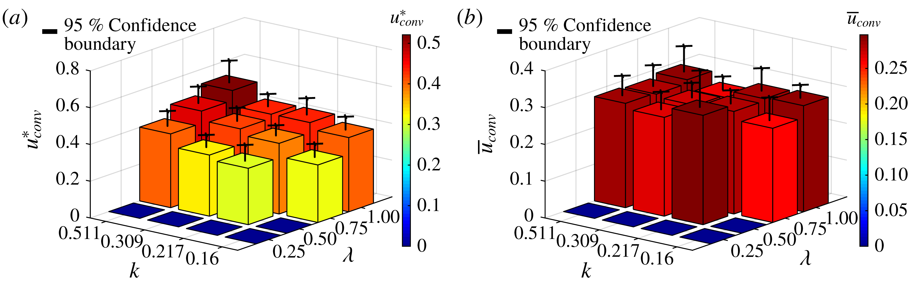
A particularly interesting result is found when convection speeds are normalized by flow conditions at the time of convection. This normalization is found by first calculating the average convection time
 $t_{conv}^{\ast }$
for each run. Converting this into dimensional time
 $t_{conv}=t_{conv}^{\ast }c/v_{0}$
, the velocity of the wing
 $v(t_{conv})$
at convection can be found from the definition of the kinematics for that case. The dimensional convection time is then normalized by this velocity at the time of convection such that
 $$\begin{eqnarray}\bar{u}_{conv}=\frac{u_{conv}^{\ast }v_{0}}{v(t_{conv})}=\frac{u_{conv}}{v(t_{conv})}.\end{eqnarray}$$
The values of this flow-normalized convection speed,
 $\bar{u}_{conv}$
, were calculated for each run and averaged for each case. The result, shown in figure 11(b), suggests that there is little variation in the ratio of convection speed to local flow velocity with either the amplitude ratio or reduced frequency of the kinematics. The results of this experiment therefore suggest that the pressure wave convection speed is some constant fraction near 28 % of the local flow velocity at the time of convection, and is invariant with cycle amplitude or frequency. In general, this fraction may vary with angle of attack; the data shown here are all for
 $\unicode[STIX]{x1D6FC}=25^{\circ }$
. If this observation holds for other angles, it would provide one piece of information helpful in modelling and predicting the flow over surging wings at high incidence. The convection speed, however, is not the only important parameter of a surging flow; the origin of the suction wave and the behaviour of the flow after convection must also be investigated.
Evolution of LEV and suction wave with
 $k=0.309$
and
 $\unicode[STIX]{x1D706}=0.75$
, viewed with the vorticity field, velocity field and surface pressure measurements.

3.5 Velocity and vorticity fields
More information about the pressure wave can be obtained by relating the pressure signals to flow field measurements obtained via PIV. For the case where
 $\unicode[STIX]{x1D706}=0.75$
and
 $k=0.309$
, the phase averaged velocity field, vorticity field and pressure measurements are plotted for multiple phase angles in figure 12. At
 $\unicode[STIX]{x1D719}=180^{\circ }$
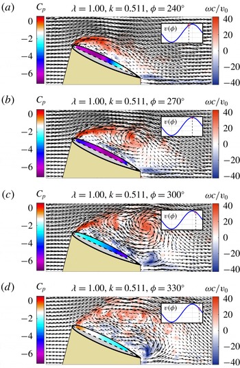
, (when the wing is accelerating and at the average velocity), the vorticity field reveals a shear layer that separates close to the leading edge and reattaches to the aerofoil before the midchord. During this initial stage of flow separation, a small low pressure region can be seen near the leading edge of the wing under the separated shear layer. This leading-edge suction peak is a result of the small region of recirculating flow that forms in this area. By
 $\unicode[STIX]{x1D719}=210^{\circ }$
, the shear layer has rolled up into a leading edge vortex (LEV) and the low pressure region on the aerofoil has grown in both in strength and size. Note that as the LEV develops and moves downstream, the pressure distribution along the aerofoil does not have a sharp suction peak directly under the vortex, but rather a relatively large region of low pressure under the area of recirculation. The process of flow separation, LEV formation, and the resulting low pressure regions observed here are very similar to those reported previously on pitching wings by Mulleners & Raffel (Reference Mulleners and Raffel2012, Reference Mulleners and Raffel2013) and Visbal & Garmann (Reference Visbal and Garmann2018) in their detailed studies of the onset of dynamic stall. Note that while the flow field images shown here are phase averaged and thus the small-scale flow structures are indistinct, in instantaneous images (see, for example, Mulleners & Raffel Reference Mulleners and Raffel2012, Reference Mulleners and Raffel2013; Visbal & Garmann Reference Visbal and Garmann2018), it is clear that both the separated shear layer and the LEV are made up of small-scale vortices and there exist small regions of secondary vorticity along the surface of the wing underneath the separated flow. While some work has suggested that the minimum surface pressure on the wing occurs directly underneath the LEV (Visbal & Garmann Reference Visbal and Garmann2018), others report that due to localized flow reversal and small regions of alternating favourable/adverse pressure gradients, the minimum surface pressure on the wing may be upstream of the LEV (Eslam Panah, Akkala & Buchholz Reference Eslam Panah, Akkala and Buchholz2015; Akkala & Buchholz Reference Akkala and Buchholz2017). The precise location of the minimum pressure is likely to be a function of the balance of circulatory (e.g. the LEV) and non-circulatory effects, and therefore a function of the reduced frequency of motion. In the current work, the minimum surface pressure appears to occur upstream of the centre of the LEV (see figure 12), but underneath the larger recirculating vortex structure. As the surging motion continues to larger
 $\unicode[STIX]{x1D719}$
, it can be seen that at
 $\unicode[STIX]{x1D719}=240^{\circ }$
the LEV has convected significantly downstream, almost off of the aerofoil, and the low pressure region has expanded with it. At
 $\unicode[STIX]{x1D719}=270^{\circ }$
, (the maximum velocity portion of the cycle), the LEV has mostly dissipated and the suction wave has passed, leaving behind a weaker suction pressure that is relatively constant over the wing chord. Here, where the LEV is larger, the small-scale structures that make up the LEV are more visible in the phase averaged flow fields. At this point in time, and for the remainder of the cycle, flow over the aerofoil is largely separated, with clear reversal along the wing surface.
Vorticity field, velocity field and surface pressure measurements for case
 $k=0.16$
and
 $\unicode[STIX]{x1D706}=1.00$
.

The pressure contours previously given in figure 10 can be more fully understood using the flow field images as a guide. For example, in the pressure contours for the
 $k=0.309$
,
 $\unicode[STIX]{x1D706}=0.75$
case, we see a linear convection of the suction wave that begins at
 $\unicode[STIX]{x1D719}=180^{\circ }$
and reaches the final sensor at approximately
 $\unicode[STIX]{x1D719}=240^{\circ }$
. This corresponds to the development and passage of the LEV in the flow field images of figure 13. The region of large suction caused by the LEV and associated recirculating flow (shown in dark blue), fades to weaker suction as the LEV dissipates and the wing enters full stall, indicated by a lack of pressure change over both chord and cycle time (a large region of solid light blue).
Examining all the pressure contours of figure 10 in this context reveals an important point: cycles at lower reduced frequencies spend a greater portion of the cycle in a fully stalled state. In the case of
 $k=0.16$
,
 $\unicode[STIX]{x1D706}=1$
, shown in figure 13, the wing enters a fully stalled condition without a strong LEV immediately after the first pressure wave, and remains there from about
 $\unicode[STIX]{x1D719}=225^{\circ }$
to
 $\unicode[STIX]{x1D719}=330^{\circ }$
, with only two small vortices providing additional suction during this period. In contrast, at an equal
 $\unicode[STIX]{x1D706}$
but greater reduced frequency,
 $k=0.511$
, the pressure contour reveals a stronger suction peak that lasts for a large portion of the cycle; little cycle time is spent fully stalled. This relationship is very important, as the fully stalled state present at low reduced frequencies represents a condition with a large amount of drag but low lift.
(a) Lift and drag decomposition of phase averaged force measurements for sample cases. Note that the normalization uses the mean velocity,
 $v_{0}$
. (b) The lift-to-drag ratio plotted from
 $\unicode[STIX]{x1D719}=150^{\circ }$
to
 $\unicode[STIX]{x1D719}=360^{\circ }$
for sample cases.

3.6 Lift-to-drag ratio
The effect of the LEV and the stalled state can be clearly seen in lift and drag decompositions of the force measurements. These are given for sample cases in figure 14(a). In the case
 $k=0.309$
and
 $\unicode[STIX]{x1D706}=0.75$
, recall that the pressure signals indicated the start of vortex convection at
 $\unicode[STIX]{x1D719}=150^{\circ }$
. It is at this point, where the LEV is forming and beginning to convect, that the lift begins to grow rapidly without a proportional increase in drag. The flow field images show a vortex mostly convected off of the aerofoil at
 $\unicode[STIX]{x1D719}=240^{\circ }$
. It is at approximately
 $\unicode[STIX]{x1D719}=240^{\circ }$
where we see the lift measurements begin to level off after the rapid increase. At
 $\unicode[STIX]{x1D719}=270^{\circ }$
, the flow fields show the wing in full stall, and it is at
 $\unicode[STIX]{x1D719}=270^{\circ }$
where we see the lift begin to decrease steadily.
If we look specifically at the lift-to-drag ratio during this portion of the cycle, shown in figure 14(b), we see that it is greatest in the period of LEV formation and convection, but drops off sharply at
 $\unicode[STIX]{x1D719}=240^{\circ }$
, where the LEV begins to convect off of the wing. The presence of the LEV over the wing is therefore a major contributor to the lift-to-drag ratio.
With equal amplitude and lower reduced frequency (
 $k=0.16$
), the pressure contour in figure 10 indicates a longer period of full stall (more area of constant colour in both the chord and phase directions), with the suction wave hitting the final sensor at about
 $\unicode[STIX]{x1D719}=210^{\circ }$
. Similarly, for this case we see the lift level off at about
 $\unicode[STIX]{x1D719}=210^{\circ }$
, and the lift-to-drag ratio falls steadily at this point. The drop in the lift-to-drag ratio begins earlier in this cycle than in the higher-frequency case (at about
 $\unicode[STIX]{x1D719}=200^{\circ }$
rather than
 $\unicode[STIX]{x1D719}=240^{\circ }$
) and also occurs more gradually than in the high-frequency case. Additionally, the magnitude of the lift coefficient is not as high as that of the higher frequency case; the pressure contours indicate weaker suction at lower frequencies.
Vorticity field, velocity field and surface pressure measurements for
 $k=0.511$
,
 $\unicode[STIX]{x1D706}=1$
.

It therefore follows that, in order to maximize the lift-to-drag ratio over a cycle (in a flapping-wing application, for example), the LEV should be over the wing for as long as possible. The highest frequency case, shown in figure 15, accomplishes this well. As in other tests, the suction wave starts at about
 $\unicode[STIX]{x1D719}=150^{\circ }$
, with a strong LEV appearing at
 $\unicode[STIX]{x1D719}=240^{\circ }$
. In this case, the LEV remains over the aerofoil until slightly after
 $\unicode[STIX]{x1D719}=300^{\circ }$
– much later in the cycle than for lower-frequency tests. At this point in the cycle, the wing is decelerating rapidly, so the vortex (which has begun to dissipate) does not convect fully into the wake, but instead its remnants move toward the leading edge (as seen at
 $\unicode[STIX]{x1D719}=330^{\circ }$
). In this case, the wing never encounters the fully stalled condition seen in lower-frequency cases. However, the stagnation of the wake over the wing induces a reverse flow on the aerofoil’s surface, causing suction pressure to remain past the midchord. While its origin is different and it acts on a smaller portion of the wing, this suction is similar to the pressure distribution caused by full stall. The stagnation of the wake is therefore undesirable, and because the wake stagnation is caused by the high-frequency motion, this case is at a higher than optimal frequency. At an ideal frequency, the wing would cleanly shed the LEV into the wake and quickly return to conditions with less suction pressure throughout the entire wing.
However, the prolonged presence of the LEV over the wing has benefits that outweigh this effect. Figure 16 presents the average lift-to-drag ratios
 $(L/D)_{avg}$
of each case from the beginning of convection (
 $\unicode[STIX]{x1D719}\approx 150^{\circ }$
) to the end of the cycle, including the 95 % confidence interval. This phase range was selected to avoid singularities at
 $\unicode[STIX]{x1D719}=90^{\circ }$
in the high
 $\unicode[STIX]{x1D706}$
cases. Also note that measurement saturation occurred in cases with
 $\unicode[STIX]{x1D706}=1$
,
 $k=0.309$
and
 $k=0.511$
, so results from these cases are not presented. At every amplitude ratio tested, higher reduced frequencies resulted in greater
 $(L/D)_{avg}$
. Restated, this is because it takes most or all of the high velocity portion of the cycle for the LEV to convect in a high-frequency case, whereas at low frequency, the LEV convects quickly and the wing is left in full stall for much of the cycle. In the current experiments, high
 $(L/D)_{avg}$
is achieved via a phenomenon very similar to wake capture, which has been studied extensively in the context of flapping wings. (See, for example, Dickinson, Lehmann & Sane Reference Dickinson, Lehmann and Sane1999; Srygley & Thomas Reference Srygley and Thomas2002; Birch & Dickinson Reference Birch and Dickinson2003; Lua, Lim & Yeo Reference Lua, Lim and Yeo2011.) Figure 16 reveals a clear maximum average lift-to-drag ratio in the case where
 $\unicode[STIX]{x1D706}=0.5$
,
 $k=0.511$
. Recall that, as shown in figure 11(a), this case at low
 $\unicode[STIX]{x1D706}$
has a slower convection speed than cases of equal frequency at higher
 $\unicode[STIX]{x1D706}$
. This lower convection speed allows the LEV to be present over a longer portion of the cycle than a higher amplitude case with faster convection speeds. Because of this, and reduced drag at lower speeds, the net effect is a better lift-to-drag ratio, even though this LEV is weaker than one created by a higher amplitude cycle. The current results agree with the work of both Maresca et al. (Reference Maresca, Favier and Rebont1979) and Choi, Colonius & Williams (Reference Choi, Colonius and Williams2015), both of whom reported achieving resonance-like phenomena on surging wings through proper selection of the amplitude and frequency. In fact, Maresca et al. (Reference Maresca, Favier and Rebont1979) reported an optimum ratio of velocity amplitude to reduced frequency,
 $\unicode[STIX]{x1D716}=\unicode[STIX]{x1D706}/k\approx 1$
;
 $\unicode[STIX]{x1D716}=0.98$
for the optimum found in the current test matrix. Choi et al. (Reference Choi, Colonius and Williams2015) found that the parameter that governs the formation of the LEV is the reduced frequency,
 $k$
. On a flat plate at
 $\unicode[STIX]{x1D6FC}=15^{\circ }$
, they found that the separation streamline emanating from the leading edge did not reattach for motions where
 $k$
was less than 0.5. A stagnation point appeared at the trailing edge when
 $k$
was increased to 0.5, and moved forward as
 $k$
was increased further. Both of these results support the optimum
 $L/D$
found in the present work at
 $\unicode[STIX]{x1D706}=0.5$
,
 $k=0.511$
. Furthermore, for sinusoidal kinematics of the type used here, it can be shown that
 $\unicode[STIX]{x1D716}=\unicode[STIX]{x1D706}/k=A/c$
, where
 $A$
is the amplitude of the wing motion (i.e. the stroke length in meters). This provides some physical intuition for the optimal motion – it is the stroke whose length allows the LEV to be cleanly shed into the wake. Longer strokes result in deep stall; shorter strokes cause the LEV to stagnate over wing during deceleration, resulting in a loss of lift similar to that caused by stall.
Average lift-to-drag ratio from
 $\unicode[STIX]{x1D719}=150^{\circ }$
to
 $\unicode[STIX]{x1D719}=360^{\circ }$
for each case.

3.7 Reverse flow results
Additional tests were performed in reverse flow, where flow separation occurs at the sharp aerodynamic leading edge (geometric trailing edge) of the wing, resulting in a flow similar to that of previous studies on flat plate wings (e.g. Taira & Colonius Reference Taira and Colonius2009; Chen, Colonius & Taira Reference Chen, Colonius and Taira2010; Pitt Ford & Babinsky Reference Pitt Ford and Babinsky2013; Mancini et al. Reference Mancini, Manar, Granlund, Ol and Jones2015; Manar & Jones Reference Manar and Jones2017). The specific wing kinematics for the current experiments were selected for comparison with the previous work of Lind et al. (Reference Lind, Trollinger, Manar, Chopra and Jones2017). Lind observed a reverse flow LEV that appeared to grow linearly in reduced time, but, as previously discussed, this LEV cannot have been a result of dynamic angle of attack change because the angle of attack was decreasing at the time the LEV formed. The current experiments focus on the time-varying free stream as an alternative cause of LEV formation and aim to determine whether the LEV observed by Lind can be recreated with a pure surge into reverse flow in the absence of rotational motion, pitch or heave.
Vorticity and velocity fields of the reverse flow experiment at
 $\unicode[STIX]{x1D706}=1.5$
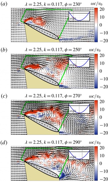
are given in figure 17. Much like on a flat plate wing at high incidence, vorticity is shed from the sharp aerodynamic leading edge as soon as the wing enters reverse flow and a shear layer forms. From
 $230^{\circ }\leqslant \unicode[STIX]{x1D719}\leqslant 250^{\circ }$
this shear layer rolls up into a coherent vortex. The vortex slowly moves closer to the aerodynamic trailing edge until approximately
 $\unicode[STIX]{x1D719}=270^{\circ }$
, when the wing begins to decelerate. By
 $\unicode[STIX]{x1D719}=290^{\circ }$
, the initial vortex has mostly shed and a weaker second vortex is forming. However, the wing’s velocity is decreasing quickly at this point, and these two vortices then stagnate over the wing and gradually decrease in strength as shown at
 $\unicode[STIX]{x1D719}=310^{\circ }$
. The stagnation of the wake over the aerofoil in this case is similar to that seen in high reduced frequencies of the full sinusoid cases.
Vorticity and velocity fields for the reverse flow test at
 $\unicode[STIX]{x1D706}=1.5$
. The relative flow is from left to right. The circulation box is shown in green.

Vorticity and velocity fields for the reverse flow test at
 $\unicode[STIX]{x1D706}=2.25$
. The relative flow is from left to right. The circulation box is shown in green.

A more aggressive case with
 $\unicode[STIX]{x1D706}=2.25$
is given in figure 18. The LEV forms much more quickly in this case and is thoroughly developed by
 $\unicode[STIX]{x1D719}=230^{\circ }$
. This initial LEV convects off the wing near
 $\unicode[STIX]{x1D719}=250^{\circ }$
, when a second vortex also begins to form. As the second vortex convects off the wing shortly after
 $\unicode[STIX]{x1D719}=270^{\circ }$
, the wing enters full stall and remains in this state until forward flow is restored. The shedding of multiple vortices and the entrance into full stall makes this flow conceptually similar to the full sinusoid cases at low reduced frequencies.
While these results do show an LEV forming from reverse flow surge at high incidence, there are some important differences between this LEV and that found on Lind’s rotor. As discussed in the introduction, Lind observed a linear increase in vortex strength with reduced time for all advance ratios tested. This result is presented graphically in figure 19(a). The vortex strength,
 $\unicode[STIX]{x1D6E4}_{\unicode[STIX]{x1D708}}$
, was computed via a summation of the positive vorticity in a circulation box:
 $$\begin{eqnarray}\unicode[STIX]{x1D6E4}_{\unicode[STIX]{x1D708}}=\int \unicode[STIX]{x1D714}^{+}\cdot \text{d}A.\end{eqnarray}$$
Reduced time is equivalent to the number of semi-chords travelled by the wing, given by
 $$\begin{eqnarray}s(t)=\frac{2}{c}\int _{0}^{t}v(t)\,\text{d}t,\end{eqnarray}$$
where
 $s=0$
at the entrance into reverse flow.
A circulation box is defined for the reverse flow surge cases of the present work, denoted by the green lines in figures 17 and 18. Using the same definition as Lind et al. (Reference Lind, Trollinger, Manar, Chopra and Jones2017), circulation is calculated in every case for each frame where the wing is within the rotor kinematics (i.e. in transition to reverse flow or in reverse flow). Plotting this circulation against reduced time yields the results shown in figure 19(b). Note that in order to match the dimensional circulation given in Lind et al. (Reference Lind, Trollinger, Manar, Chopra and Jones2017), the circulation measurements from the present work are normalized by the value of
 $cv_{0}$
from the present work, then multiplied by the value of
 $cv_{0}$
from Lind et al. (Reference Lind, Trollinger, Manar, Chopra and Jones2017).
(a) Variation of vortex strength and reduced time found for the reverse flow LEV, from Lind et al. (Reference Lind, Trollinger, Manar, Chopra and Jones2017). (b) Variation of circulation with reduced time from the surging reverse flow experiments of the present work.

There are important differences and similarities between the growth in vortex strength seen on the rotor and that observed in the surge experiments. First, the rotor LEV grows at a constant linear rate with reduced time, regardless of advance ratio (i.e. all advance ratios have equal slope in figure 19
a). However, the growth rate of the initial surging-wing LEV (the first period of linear growth for all
 $\unicode[STIX]{x1D706}$
in figure 19
b), is much greater than the growth rate of the rotor case and increases with
 $\unicode[STIX]{x1D706}$
up to
 $\unicode[STIX]{x1D706}=2$
. Because the slope of the circulation growth with reduced time does appear to converge with increased
 $\unicode[STIX]{x1D706}$
(or equivalently, increased
 $Re$
), the variance of growth rate is suspected to result from the difference in flow acceleration between the tests. In the
 $\unicode[STIX]{x1D706}=1.5$
case, the flow accelerates to a maximum Reynolds number of 30 000, while the corresponding
 $\unicode[STIX]{x1D707}=0.6$
rotor blade element accelerates to a maximum reverse flow Reynolds number of approximately 85 000. The reduced time rate of circulation growth, or equivalently, the leading-edge vorticity flux, has been shown by Manar & Jones (Reference Manar and Jones2017) to be a function of acceleration at low Reynolds numbers. It is possible that this measure of LEV growth eventually converges as the magnitude of acceleration increases. Thus, all of Lind’s rotor cases might be beyond this critical acceleration, and therefore show equal circulation growth with reduced time. The
 $\unicode[STIX]{x1D706}=1.5$
and
 $1.75$
cases of the current experiments might have acceleration below this critical level, which would explain their reduced growth with reduced time compared to the more aggressive cases. The discrepancy in growth rate magnitude, which is much greater in the surge case than in the rotor case, is suspected to be a result of the transport of vorticity along the rotor blade due to the spanwise flow that develops on the three-dimensional rotor.
Another difference of particular importance is that the rotor LEV shows continuous growth in reduced time, while the surging-wing LEV shows regions of growth, followed by periods of decline. Physically, the increase of
 $\unicode[STIX]{x1D6E4}$
corresponds to portions of the cycle when the LEV is steadily growing from the vorticity shed by the aerodynamic leading edge. Periods of decrease in
 $\unicode[STIX]{x1D6E4}$
indicate the convection of a vortex into the wake, as the positive vorticity associated with it moves out of the circulation box. This is a quantitative approach to describing what we already knew from analysis of the flow field images – that in all but the
 $\unicode[STIX]{x1D706}=1.5$
case the primary LEV fully convects into the wake (seen as a
 $\unicode[STIX]{x1D6E4}$
decrease), and is then followed by the formation of a second vortex (
 $\unicode[STIX]{x1D6E4}$
increase). This difference makes Lind’s data quite remarkable; it suggests that the LEV formed in the rotary surge into reverse flow does not convect as far or as fast as the LEV resulting from an equivalent pure surge does. In other words, rotary motion has a stabilizing effect on the reverse flow LEV. This result is already well established in research of flapping-wing aerodynamics, but its application to rotorcraft is not commonly realized. Thus, a large body of research on the stability of LEVs in the context of rotating and flapping wings may also be applicable to the reverse flow LEV observed on rotorcraft. (See, for example, Birch & Dickinson Reference Birch and Dickinson2001; Shyy et al.
Reference Shyy, Trizila, Kang and Aono2009; Carr & Ringuette Reference Carr and Ringuette2014; Garmann & Visbal Reference Garmann and Visbal2014; Wojcik & Buchholz Reference Wojcik and Buchholz2014; Wolfinger & Rockwell Reference Wolfinger and Rockwell2014; Manar et al.
Reference Manar, Mancini, Mayo and Jones2016; Medina & Jones Reference Medina and Jones2016; Jardin Reference Jardin2017; Eldredge & Jones Reference Eldredge and Jones2019.) On relatively low Reynolds number flapping and rotating wings, LEV attachment is achieved through a balance of vorticity transport mechanisms: convection, stretching, Coriolis tilting and annihilation (Wojcik & Buchholz Reference Wojcik and Buchholz2014; Jardin Reference Jardin2017). However, due to radial variations in the local velocity of a rotating wing, the relative strengths of these effects vary along the wing span in different ways. It remains to be seen how the balance of vorticity generation and transport shifts at the much greater Reynolds numbers typical of full-scale rotorcraft.
Among the many differences, a remarkable similarity between the rotor LEV and the reverse flow surge LEV is also present. The peak circulation measurements from reverse flow surge are of similar magnitude to the corresponding rotor cases. For rotor cases
 $\unicode[STIX]{x1D707}=\{0.6,0.7,0.8,0.9\}$
corresponding to surge cases
 $\unicode[STIX]{x1D706}=\{1.5,1.75,2.0,2.25\}$
, the per cent difference between the maximum vortex strength in the rotor experiment and the maximum circulation in the surge experiment is
 $\{2.5\,\%,11\,\%,22\,\%,1.1\,\%\}$
. While we cannot be sure that the rotor LEVs in Lind et al. (Reference Lind, Trollinger, Manar, Chopra and Jones2017) have reached their peak strength before data collection ends (at the maximum reduced time), we can expect, since the flow has begun to decelerate by that point, that any further growth would be limited. (Additional growth from rotor LEVs would also decrease the reported differences.) Thus, while the characteristics of the LEV in surge are not precisely the same as the rotor LEV (i.e. the vortex remains attached on the rotor, but not on the surging wing), the maximum strength of a reverse flow LEV might be reasonably approximated by a pure surge with equivalent reduced frequency and amplitude ratio.
4 Conclusion
4.1 Full sinusoid tests
Experiments on surging wings in a water tank demonstrated that large-scale flow separation and vortex formation occurs at high incidence, the process of which bears many similarities to the onset of dynamic stall on pitching wings. The full sinusoid surging-wing results presented here demonstrate the balance between amplitude ratio and reduced frequency in surging wings. Higher-frequency oscillations have shorter cycles, allowing the LEV to be over the wing for a greater fraction of the cycle, whereas low-frequency cycles experience full stall after the LEV sheds from the wing. Higher-frequency cycles also have greater LEV strength, increasing the lift resulting from the LEV. High amplitude cycles create a stronger LEV, but also show slightly faster LEV convection times, so that the LEV is over the wing for less of the cycle. This, coupled with additional drag in high amplitude cases, can result in a reduction of
 $(L/D)_{avg}$
with increased amplitude in some cases.
Analysis of convection speeds suggests that the LEV’s convection velocity at a fixed angle of attack is a constant fraction of the free-stream velocity at the time of convection. If this relationship is true for a broad angle of attack range, and the phase of convection can be predicted, it could form the basis for a reliable model of force production. If the goal is to maximize
 $(L/D)_{avg}$
in each cycle, these results suggest it is most important to pick a reduced frequency that maximizes the amount of cycle time where the LEV is over the wing, yet allows the LEV to convect into the wake rather than weaken and stagnate over the wing.
Depending on the application, this optimal reduced frequency could be estimated based on the assumption that the LEV convects at a constant fraction of the local stream velocity at the time of convection. Using the current problem as an example, the results showed a convection speed ratio
 $\bar{u}_{conv}\approx 0.28$
for all cases. Using the average phase of convection from the
 $k=0.309$
,
 $\unicode[STIX]{x1D706}=0.5$
case,
 $\unicode[STIX]{x1D719}\approx 210^{\circ }$
, we know the wing’s velocity at convection to be
 $v(\unicode[STIX]{x1D719}=210^{\circ })=0.474~\text{m}~\text{s}^{-1}$
. The velocity of the LEV over the wing is then approximately
 $u_{conv}\approx 0.133~\text{m}~\text{s}^{-1}$
. The wing’s chord is
 $c=0.1047~\text{m}$
, so the LEV will convect in approximately 0.79 s. For this length of time to pass in a sinusoidal free stream between approximately
 $\unicode[STIX]{x1D719}=180^{\circ }$
(where we know the vortex to form) and
 $\unicode[STIX]{x1D719}=330^{\circ }$
(where we might like the vortex to have shed), would require a full cycle length of
 $T=1.90~\text{s}$
. With this wing’s chord and the mean velocity of these kinematics, this translates into a reduced frequency of
 $k=0.45$
. These are rough calculations, but measurements of the cases with
 $\unicode[STIX]{x1D706}=0.5$
case do show a very large
 $(L/D)_{avg}$
at
 $k=0.511$
, which is not far from the result of this estimate,
 $k=0.45$
. Based on the flow field images, it was also proposed that the
 $k=0.511$
case is at a higher frequency than optimum due to the stagnation of the weakening LEV over the wing.
There are, however, some complications. Here, the phase of convection is experimentally measured, but in a design situation there is an additional challenge of predicting when convection occurs. A full model would also need to include a means of estimating the LEV strength to predict the
 $(L/D)_{avg}$
– not simply an estimate of the kinematics that would maximize it. Finally, most applications include flow elements other than surge that may greatly alter the convection speed of the vortex (e.g. rotary motion). Still, with refinement a method of this type could show promise.
4.2 Reverse flow
Results of the reverse flow experiments described here show that high incidence surge of the rotor blade into reverse flow may have been the source of the reverse flow LEV previously observed by Lind et al. (Reference Lind, Trollinger, Manar, Chopra and Jones2017). However, in the present case of pure surge, the LEV was found to shed from the wing and convect into the wake while the rotor LEV did not. Rotary motion could therefore be described as having a stabilizing effect on the reverse flow LEV, much like that previously observed on rotating wings at much lower Reynolds numbers in the context of flapping wings and micro air vehicles.
The maximum vortex strengths measured in pure reverse flow surge were similar to the maximum vortex strengths measured for the rotor. This result, combined with the observation of linear vortex growth in reduced time from Lind et al. (Reference Lind, Trollinger, Manar, Chopra and Jones2017), could form the basis for a low-order model of LEV formation in separated three-dimensional and rotary flows. For example, for a blade element of a particular rotor (or other lifting surface at high incidence), the maximum vortex strength
 $\unicode[STIX]{x1D6E4}_{max}$
might be estimated from a corresponding case of pure surge as detailed in the present work. Then, one might assume a linear growth in circulation with reduced time from (
 $s=0$
,
 $\unicode[STIX]{x1D6E4}=0$
), to (
 $s_{max}$
,
 $\unicode[STIX]{x1D6E4}_{max}$
), where
 $s_{max}$
is the reduced time at which
 $\unicode[STIX]{x1D6E4}$
is maximized (likely corresponding to a time not far after the maximum reverse flow velocity). Some approximation would also have to be made for the decrease in circulation from
 $s=s_{max}$
to the exit of the reverse flow region (or cessation of wing motion). If circulation near the blade can be estimated in the presence of separated flow and a strong LEV, estimations of surface pressures and forces would shortly follow.
4.3 Future work
There is much further investigation required in the convection of surging-wing LEVs. First, a study of the variation of LEV convection speed with static angle of attack would further expand upon a major observation in this experiment – that LEV convection speed is a constant ratio of the local free-stream velocity. It is likely that if a constant convection speed ratio can be found for all angles of attack, the ratio itself is a function of angle of attack. Secondly, a study at fixed amplitude and many variations of frequency could help to pinpoint exactly what conditions produce optimum
 $(L/D)_{avg}$
. Flow field images and pressure distributions of a case with maximum
 $(L/D)_{avg}$
would provide a better qualitative understanding of the ideal flow structure, including at what point in the cycle the LEV should convect to avoid stagnating over the wing. Finally, a specific study of convection speed in various rotary motions would test the observations of these fundamental experiments in kinematics closer to a final application. A greater range of experimental comparison is needed between the surging-wing LEV and more practical applications such as the reverse flow LEV found on high-advance-ratio rotors. If the similarity in maximum circulation between these cases can be verified over a wider range of parameters, work can begin on the formation of a low-order flow model based on canonical kinematics.
Acknowledgements
This work was supported in part by the National Science Foundation under grant 1553970 and the US Army/Navy/NASA Vertical Lift Research Center of Excellence Cooperative Agreement with M. Bhagwat serving as Program Manager and Technical Agent, grant number W911W6-17-2-0004. The authors would also like to thank Dr F. Lagor for the design and construction of the model used in the reverse flow experiments.