


1. Introduction
Thermal convection is ubiquitous in nature and finds its application in industries, in the atmosphere, in the mantle of the Earth and inside stars, to name a few (Ahlers, Grossmann & Lohse Reference Ahlers, Grossmann and Lohse2009; Chilla & Schumacher Reference Chilla and Schumacher2012; Doering Reference Doering2020). Rayleigh–Bénard convection (RBC) is an ideal system to study thermal convection, where heat transfer takes place in a horizontal layer confined by two isothermal plates. Here, buoyancy triggers instability in the flow that sets the motion in the convection cell, resulting in an upward and downward movement of hot and cold fluid, respectively. Generally, RBC refers to a convection cell of smooth walls with a vertical temperature gradient parallel to the gravity. However, real-life situations are different. For instance, the presence of asperities on the surfaces and flow inside an inclined cell are some common considerations that can be seen in reality (Toppaladoddi, Succi & Wettlaufer Reference Toppaladoddi, Succi and Wettlaufer2015; Chand, De & Mishra Reference Chand, De and Mishra2021b; Toppaladoddi et al. Reference Toppaladoddi, Wells, Doering and Wettlaufer2021). Owing to the application of thermal convection in industrial processes, heat exchangers and flow circulation in the atmosphere, these variants of RBC can be used to enhance heat transfer. Such practical situations have motivated us to study the tilted variant of RBC with and without rough surfaces. Based on the inclination angle  $\phi$, the tilted RBC can be categorized into three cases: RBC at
 $\phi =0^{\circ }$ or the level case (Shraiman & Siggia Reference Shraiman and Siggia1990; Johnston & Doering Reference Johnston and Doering2009; Chand et al. Reference Chand, Sharma, Venugopal and De2019; Vishnu, De & Mishra Reference Vishnu, De and Mishra2020), vertical convection (VC) at
 $\phi =90^{\circ }$ (Ng et al. Reference Ng, Ooi, Lohse and Chung2015; Shishkina Reference Shishkina2016; Wang et al. Reference Wang, Liu, Verzicco, Shishkina and Lohse2021), and inclined convection (IC) for
 $0^{\circ } < \phi < 90^{\circ }$ (Riedinger et al. Reference Riedinger, Tisserand, Seychelles, Castaing and Chilla2013; Kolesnichenko et al. Reference Kolesnichenko, Mamykin, Pavlinov, Pakholkov, Rogozhkin, Frick, Khalilov and Shepelev2015).
In RBC, there are three main flow control parameters: Rayleigh number ( $Ra$), Prandtl number (
 $Pr$) and aspect ratio (
 $\varGamma$). While Rayleigh number
 $Ra=g\beta \,\Delta T\, H^{3}/(\nu \alpha )$ is the vertical thermal forcing applied across the isothermal surfaces, and Prandtl number
 $\nu /\alpha$ is a property of fluid, aspect ratio
 $L/H$ is a geometric parameter of the convection cell whose height and width are represented by
 $H$ and
 $L$. Here,
 $g$ is gravitational acceleration,
 $\Delta T$ is the temperature difference between the two isothermal surfaces, and
 $\beta$,
 $\nu$ and
 $\alpha$ are coefficients of thermal expansion, kinematic viscosity and thermal diffusivity of the fluid, respectively. The two response parameters are heat flux and flow strength, which are represented in non-dimensional form by Nusselt number
 $Nu$ and Reynolds number
 $Re$, respectively. These response parameters exhibit power-law behaviour with
 $Ra$ and
 $Pr$ (Malkus & Chandrasekhar Reference Malkus and Chandrasekhar1954; Castaing et al. Reference Castaing, Gunaratne, Heslot, Kadanoff, Libchaber, Thomae, Wu and Zanetti1989; Doering Reference Doering2020). Several experimental, numerical and theoretical studies have revealed the Rayleigh number dependence of heat flux
 $Nu$ (Malkus & Chandrasekhar Reference Malkus and Chandrasekhar1954; Priestley Reference Priestley1954; Kraichnan Reference Kraichnan1962; Howard Reference Howard1963; Spiegel Reference Spiegel1963; Verzicco & Camussi Reference Verzicco and Camussi1999; Doering Reference Doering2019). Malkus & Chandrasekhar (Reference Malkus and Chandrasekhar1954) proposed the classical scaling theory
 $Nu \sim Ra^{1/3}$. For extremely large
 $Ra$, Kraichnan (Reference Kraichnan1962) prescribed the corrected asymptotic law
 $Nu\sim [Ra/(\ln Ra)^{3}]^{1/2}$. Using the idea of the mixing-layer hypothesis, Castaing et al. (Reference Castaing, Gunaratne, Heslot, Kadanoff, Libchaber, Thomae, Wu and Zanetti1989) proposed that
 $Nu \sim Ra^{2/7}$. In a numerical investigation on the
 $Nu(Pr)$ dependence, Verzicco & Camussi (Reference Verzicco and Camussi1999) identified the critical
 $Pr=0.35$, which demarcates two regimes. While heat flux increases with
 $Pr$ for
 $Pr\leq 0.35$, it becomes independent beyond the critical
 $Pr$. Grossmann & Lohse (Reference Grossmann and Lohse2000) provided a unified view to the
 $Ra$ and
 $Pr$ dependence of Nusselt number. On the other hand, in VC, the
 $Nu(Ra)$ scaling yields
 $1/4$ (Schmidt & Beckmann Reference Schmidt and Beckmann1930; Saunders & Tizard Reference Saunders and Tizard1939; Churchill & Chu Reference Churchill and Chu1975) and
 $1/3$ (Fujii et al. Reference Fujii, Takeuchi, Fujii, Suzaki and Uehara1970; George & Capp Reference George and Capp1979) exponents in low and high
 $Ra$ regimes, respectively. Since enhancing heat flux is one of the main objectives, altering certain geometrical aspects of a convection cell and plume emission process can yield higher heat flux (Roche et al. Reference Roche, Castaing, Chabaud and Hébral2001; Stringano, Pascazio & Verzicco Reference Stringano, Pascazio and Verzicco2006; Toppaladoddi et al. Reference Toppaladoddi, Succi and Wettlaufer2015). Recently, rough surface has been exploited to achieve the enhanced heat flux (Toppaladoddi, Succi & Wettlaufer Reference Toppaladoddi, Succi and Wettlaufer2017; Zhang et al. Reference Zhang, Sun, Bao and Zhou2018; Chand, Sharma & De Reference Chand, Sharma and De2021a; Chand et al. Reference Chand, De and Mishra2021b; Toppaladoddi et al. Reference Toppaladoddi, Wells, Doering and Wettlaufer2021). Toppaladoddi et al. (Reference Toppaladoddi, Succi and Wettlaufer2017) reported augmented heat flux due to a surge in emission of thermal plumes. Zhang et al. (Reference Zhang, Sun, Bao and Zhou2018) and Chand et al. (Reference Chand, Sharma and De2021a) identified the critical roughness height and critical Rayleigh number, respectively, beyond which heat flux increases.
Apart from the flow-governing parameters and surface roughness, inclination of a convection cell can also enhance the heat transport (Dropkin & Somerscales Reference Dropkin and Somerscales1965; Langebach & Haberstroh Reference Langebach and Haberstroh2014). However, the enhancement depends strictly upon the governing parameters, which are described in detail later. On account of buoyancy, inclination induces characteristics of shear flow. This setting of heat transfer enhancement has been studied extensively over the years in both two- and three-dimensional geometries (Xin & Le Quere Reference Xin and Le Quere1995; Zwirner & Shishkina Reference Zwirner and Shishkina2018; Wang et al. Reference Wang, Wan, Yan and Sun2019; Zhang et al. Reference Zhang, Chen, Xia, Xi, Zhou and Chen2021). In an experimental study over different inclination angles, Dropkin & Somerscales (Reference Dropkin and Somerscales1965) observed that the  $Nu(Ra)$ scaling exponent does not change with
 $\phi$, and the variation in heat flux occurs due to different prefactors. In a small inclination range and water-filled cylindrical cells, Chilla et al. (Reference Chilla, Rastello, Chaumat and Castaing2004), Sun, Xi & Xia (Reference Sun, Xi and Xia2005) and Ahlers, Brown & Nikolaenko (Reference Ahlers, Brown and Nikolaenko2006) observed a drop in heat flux as the convection cell is tilted, due to the attributes of large-scale rolls and transformation of flow states from a single-roll to a double-roll state. While Chilla et al. (Reference Chilla, Rastello, Chaumat and Castaing2004) and Sun et al. (Reference Sun, Xi and Xia2005) studied in aspect ratio one-half, Ahlers et al. (Reference Ahlers, Brown and Nikolaenko2006) investigated in a unit aspect ratio. For nearly the same governing parameters as in Ahlers et al. (Reference Ahlers, Brown and Nikolaenko2006), Weiss & Ahlers (Reference Weiss and Ahlers2013) observed a slight increment in heat flux for a confined geometry of
 $\varGamma =1/2$ due to the dominance of a single-roll state over a double-roll state.
For very-low-Prandtl-number fluid ( $Pr=0.0094$), Frick et al. (Reference Frick, Khalilov, Kolesnichenko, Mamykin, Pakholkov, Pavlinov and Rogozhkin2015) investigated the flow dynamics for
 $2\times 10^{6} \leq Ra \leq 10^{7}$ at four inclined angles, namely
 $0^{\circ }$,
 $2^{\circ }$,
 $45^{\circ }$ and
 $90^{\circ }$. This study suggested that thermal plumes carry heat at small inclination angles, while large-scale circulation (LSC) carries it at larger angles. The
 $Nu$ obtained at
 $\phi =90^{\circ }$ was found greater than that in the level case, which shows that LSC carries the heat more efficiently than thermal plumes. Using the same working fluid in a cylindrical cell of
 $\varGamma =1/20$, Vasilev et al. (Reference Vasilev, Kolesnichenko, Mamykin, Frick, Khalilov, Rogozhkin and Pakholkov2015) obtained the maximum
 $Nu$ at
 $\phi =65^{\circ }$, which confirms the higher efficiency of LSC. In a recent study, Khalilov et al. (Reference Khalilov, Kolesnichenko, Pavlinov, Mamykin, Shestakov and Frick2018) used the same working fluid in a unit-aspect-ratio cylindrical cell, and found contrasting results. They observed a weak
 $Nu(\phi )$ dependency, although the trend remained the same where maximum heat flux was obtained at
 $\phi =70^{\circ }$. All these studies reveal the unimodal characteristic of the
 $Nu\unicode{x2013}\phi$ curve, where the maximum heat transfer occurs around
 $\phi \approx 70^{\circ }$.
In a quasi-two-dimensional cubic cell filled with water ( $Pr=6.3$), Guo et al. (Reference Guo, Zhou, Cen, Qu, Lu, Sun and Shang2015) reported a monotonically decreasing trend of
 $Nu\unicode{x2013}\phi$ with three slopes, the maximum being in the range
 $60^{\circ }\unicode{x2013}90^{\circ }$. The maximum drop in
 $Nu$ was found to be
 $18\,\%$ for the vertical convection. In the same geometric configuration but with different parameters (
 $Ra= 6.8 \times 10^{10}$,
 $Pr\approx 10$), Guo et al. (Reference Guo, Zhou, Qu, Cen and Lu2017) observed a similar decreasing trend in
 $Nu(\phi )$. Based on the similar
 $Nu(\phi )$ trend for different fluids and thermal forcing, they concluded that the trend does not depend upon
 $Ra$ and
 $Pr$. Further, Shishkina & Horn (Reference Shishkina and Horn2016) investigated the effect of
 $Ra$ and
 $Pr$ on
 $Nu(\phi )$ and
 $Re(\phi )$ in a range of
 $Pr$ varying from
 $0.1$ to
 $100$ for
 $Ra=10^{6}$,
 $10^{7}$ and
 $10^{8}$. They suggested that the
 $Nu\unicode{x2013}\phi$ relationship is a non-monotonic function of
 $Pr$ and
 $Ra$, and does not follow a simple power law. Moreover, it was found that large (intermediate) inclination angles result in efficient heat transport in high (small)
 $Pr$ cases. In a confined cylindrical cell of
 $\varGamma =1/5$, Zwirner & Shishkina (Reference Zwirner and Shishkina2018) obtained
 $2.3$ times enhancement in heat flux (with respect to the level case) at
 $\phi =45^{\circ }$ for
 $Ra=10^{7}$ and
 $Pr=0.1$. They attributed the enhancement to a dominant single-roll state that transports heat more efficiently than a double-roll state.
Two-dimensional RBC has been used widely to understand flow dynamics (Shishkina & Wagner Reference Shishkina and Wagner2011), heat transfer (van der Poel, Stevens & Lohse Reference van der Poel, Stevens and Lohse2011, Reference van der Poel, Stevens and Lohse2013; Huang & Zhou Reference Huang and Zhou2013; van der Poel et al. Reference van der Poel, Ostilla-Mónico, Verzicco, Grossmann and Lohse2015a) and boundary layer dynamics (Zhou & Xia Reference Zhou and Xia2010; Zhou et al. Reference Zhou, Sugiyama, Stevens, Grossmann, Lohse and Xia2011; van der Poel et al. Reference van der Poel, Verzicco, Grossmann and Lohse2015b). Moreover, it has also been used to study the effect of roughness on heat flux (Toppaladoddi et al. Reference Toppaladoddi, Succi and Wettlaufer2017; Zhang et al. Reference Zhang, Sun, Bao and Zhou2018; Zhu et al. Reference Zhu, Mathai, Stevens, Verzicco and Lohse2018, Reference Zhu, Stevens, Shishkina, Verzicco and Lohse2019), and to unveil the flow dynamics in a tilted convection cell (Wang et al. Reference Wang, Xia, Wang, Sun, Zhou and Wan2018a,Reference Wang, Wan, Yan and Sunb, Reference Wang, Wan, Yan and Sun2019, Reference Wang, Liu, Verzicco, Shishkina and Lohse2021; Jiang, Sun & Calzavarini Reference Jiang, Sun and Calzavarini2019). Wang et al. (Reference Wang, Wan, Yan and Sun2018b) identified the range of aspect ratio in which tilted RBC can be used to enhance the heat flux. In another study, Wang et al. (Reference Wang, Xia, Wang, Sun, Zhou and Wan2018a) investigated flow reversals in unit- and double-aspect ratio cells. Wang et al. (Reference Wang, Wan, Yan and Sun2019) studied the effect of  $Pr$ on
 $Nu(\phi )$ and
 $Re(\phi )$ for a rectangular box of
 $\varGamma =1/2$. For a high-
 $Pr$ fluid (
 $Pr=480$), Jiang et al. (Reference Jiang, Sun and Calzavarini2019) studied the
 $Nu(\phi )$ trend for
 $Ra=10^{8}$ and
 $5\times 10^{8}$. Note that although the real flow situation would be three-dimensional, we investigate the effect of inclination in two dimensions for two primary reasons. First, the dependence of global heat transport properties on
 $\phi$ and
 $Ra$ in two and three dimensions remains nearly the same (Zhang, Zhou & Sun Reference Zhang, Zhou and Sun2017). Second, two-dimensional simulations are computationally cheaper, which has resulted in a series of simulations that produced a fuller data set for all the predictions and power-law behaviour.
It is clear from the literature that IC yields greater heat flux than RBC and VC (Frick et al. Reference Frick, Khalilov, Kolesnichenko, Mamykin, Pakholkov, Pavlinov and Rogozhkin2015; Shishkina & Horn Reference Shishkina and Horn2016; Jiang et al. Reference Jiang, Sun and Calzavarini2019; Wang et al. Reference Wang, Wan, Yan and Sun2019). However, a unified view for the inclination angle that yields maximum heat flux remains elusive, which was also suggested by Shishkina & Horn (Reference Shishkina and Horn2016). Therefore, the aim of the present work is to disentangle the Rayleigh number dependence of  $Nu(\phi )$ for a low
 $Pr=0.7$ and
 $\varGamma =2$, which has not been studied extensively so far. In the
 $Ra$ range
 $10^{6}\leq Ra\leq 10^{9}$, we identify the control parameters (
 $Ra$ and
 $\phi$) that result in enhanced heat flux for IC. To the best of our knowledge, the scaling theories for
 $Nu(Ra)$ and
 $Re(Ra)$ power laws are available only for the two extreme inclined cases, i.e. RBC (
 $\phi =0^{\circ }$; Malkus & Chandrasekhar Reference Malkus and Chandrasekhar1954; Castaing et al. Reference Castaing, Gunaratne, Heslot, Kadanoff, Libchaber, Thomae, Wu and Zanetti1989) and VC (
 $\phi =90^{\circ }$; Saunders & Tizard Reference Saunders and Tizard1939; Churchill & Chu Reference Churchill and Chu1975; Shishkina Reference Shishkina2016). However, in a recent study, Zhang et al. (Reference Zhang, Chen, Xia, Xi, Zhou and Chen2021) extended the Grossmann–Lohse theory for horizontal buoyancy. Considering the unavailability of the above-mentioned power laws, we report the
 $Nu(Ra)$ and
 $Re(Ra)$ scaling exponents for each inclination angle. For the first time, we report the impact of surface roughness on
 $Nu(\phi )$ and
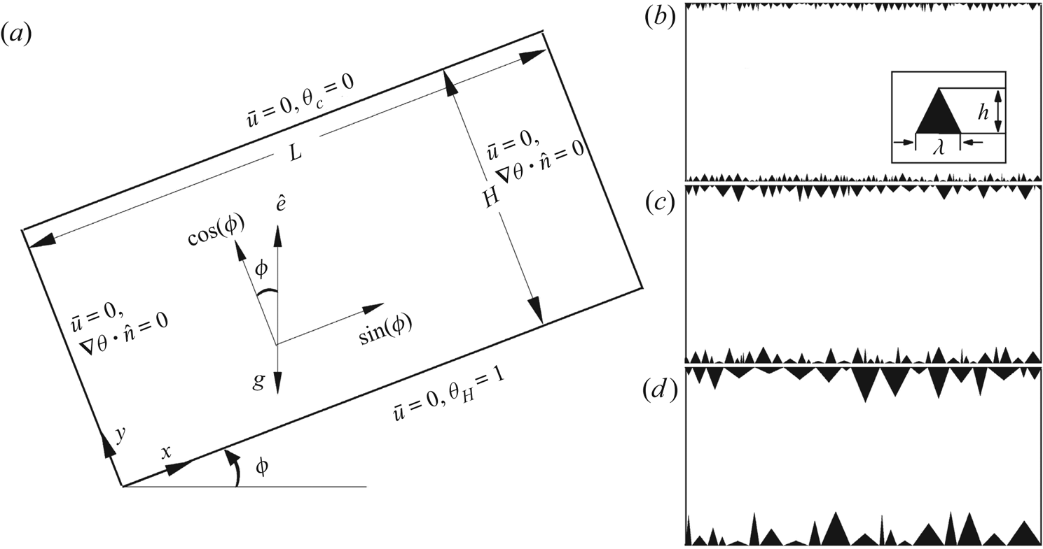
 $Re(\phi )$ using three roughness set-ups, whose schematics are shown in figure 1. Here, all three rough boundaries (irregular) are implanted on the isothermal surfaces. Note that these set-ups are characterized by the maximum height of their roughness elements, whose details are given in figure 1. Another physical argument to consider surface roughness is that it enhances the emission of thermal plumes and breaks the large-scale rolls into smaller ones, which influence the heat flux (Chand et al. Reference Chand, De and Mishra2021b). So it will be interesting to study the combined effect of roughness and tilt on global heat transport properties.
Schematic diagram of (a) the smooth tilted convection cell with boundary conditions and components of unit vector  $\hat {e}$ in the
 $x$ and
 $y$ directions, and (b) the smallest (R
 $_1$), (c) the intermediate (R
 $_2$) and (d) the tallest (R
 $_3$) rough surfaces. The inset in (b) shows the wavelength (
 $\lambda$) and height (
 $h$) of a roughness element. (a) Smooth surface; (b) smallest roughness, R
 $_1$ (
 $0.005 < h/H <0.05$); (c) intermediate roughness, R
 $_2$ (
 $0.01 < h/H <0.1$); (d) tallest roughness, R
 $_3$ (
 $0.02 < h/H <0.2$).

In most of the IC studies, confined geometries ( $\varGamma \leq 1$) have been used to realize the idea of heat flux enhancement (Chilla et al. Reference Chilla, Rastello, Chaumat and Castaing2004; Sun et al. Reference Sun, Xi and Xia2005; Ahlers et al. Reference Ahlers, Brown and Nikolaenko2006; Weiss & Ahlers Reference Weiss and Ahlers2013; Frick et al. Reference Frick, Khalilov, Kolesnichenko, Mamykin, Pakholkov, Pavlinov and Rogozhkin2015; Guo et al. Reference Guo, Zhou, Cen, Qu, Lu, Sun and Shang2015; Vasilev et al. Reference Vasilev, Kolesnichenko, Mamykin, Frick, Khalilov, Rogozhkin and Pakholkov2015; Shishkina & Horn Reference Shishkina and Horn2016; Khalilov et al. Reference Khalilov, Kolesnichenko, Pavlinov, Mamykin, Shestakov and Frick2018; Jiang et al. Reference Jiang, Sun and Calzavarini2019; Wang et al. Reference Wang, Wan, Yan and Sun2019). Since the flow in nature does not occur in the confined geometries, studies dedicated to wider convection cells are of greater interest (Wang et al. Reference Wang, Wan, Yan and Sun2018b). Moreover, Wang et al. (Reference Wang, Wan, Yan and Sun2018b) suggest that heat flux enhancement occurs only for
 $\varGamma \leq 8$. To avoid the effect of confinement due to lateral walls for
 $\varGamma <1$ and to achieve the enhanced heat flux, we have selected a relatively wider convection cell of
 $\varGamma =2$. The present study is conducted at five tilt angles (
 $\phi =0^{\circ }$,
 $15^{\circ }$,
 $45^{\circ }$,
 $75^{\circ }$ and
 $90^{\circ }$) that cover the entire inclination range. We have considered
 $\phi =15^{\circ }$ and
 $75^{\circ }$ to elucidate the competing transport mechanism between LSC and thermal plumes, and identify the most efficient state of heat transport, respectively.
The rest of the paper is organized as follows. Numerical details are provided in § 2. For the smooth case, we report the effect of inclination on flow structures, and  $Nu\unicode{x2013}\phi$ and
 $Re\unicode{x2013}\phi$ dependencies, in §§ 3.1–3.3, respectively. We explore the effect of rough surface on flow structures and global transport properties in §§ 3.4–3.6. The paper is concluded in § 4.
2. Numerical details
Figure 1 shows the schematic of a double-aspect-ratio tilted convection cell with boundary conditions and three roughness set-ups. Under the Oberbeck–Boussinesq approximation, incompressible buoyancy-driven-flows are governed by the continuity, momentum and energy equations. For a cell tilted at angle  $\phi$, the governing equations can be written in their non-dimensional form as
 $$\begin{gather} \boldsymbol{\nabla}\,\boldsymbol{\cdot}\,\bar{u}=0, \end{gather}$$
 $$\begin{gather}\frac{\partial \bar{u}}{\partial t} + \bar{u}\,\boldsymbol{\cdot}\,\boldsymbol{\nabla} \bar{u} ={-}\boldsymbol{\nabla} p + \sqrt{\frac{Pr}{Ra}}\,\nabla^{2}\bar{u} + \theta \hat{e}, \end{gather}$$
 $$\begin{gather}\frac{\partial \theta}{\partial t} + \bar{u}\,\boldsymbol{\cdot}\,\boldsymbol{\nabla} \theta = \frac{1}{\sqrt{Pr\,Ra}}\,\nabla^{2}\theta, \end{gather}$$
where  $x,y$ represent Cartesian coordinates, and
 $\bar {u}=(u,v)$,
 $p$ and
 $\theta$ are velocity, pressure and temperature, respectively. In IC, thermal forcing acts in both directions, given by
 $\hat {e}=(\sin \phi,\cos \phi )$ as shown in figure 1(a). The governing equations are non-dimensionalized by the free-fall velocity scale
 $\sqrt {g\beta \,\Delta T\,H}$, height of the convection cell
 $H$, and temperature difference
 $\theta =(T-T_C)/(T_H-T_C)$. With respect to the level case, the top and bottom surfaces are kept at isothermal temperature conditions, whereas the lateral walls are adiabatic. A no-slip velocity boundary condition is enforced on all four walls (including rough surfaces). It is not intuitive to use horizontal and vertical terminology in a tilted cell to refer to the directions along the isothermal surface and normal to it. Thus from here onwards, we indicate the direction along the isothermal surfaces as IS, and normal to them as NIS. In the present work, we compute the two response parameters
 $Nu$ and
 $Re$ as
 \begin{equation} Nu = 1+\sqrt{Ra\,Pr}\,\langle v\theta\rangle_{V,t} \quad \text{and} \quad Re= \sqrt{\frac{Ra}{Pr}}\,U, \end{equation}
where  $U=\sqrt {\langle \bar {u}\,\cdot\,\bar {u}\rangle _{V,t}}$, and
 $\langle \,\cdot\, \rangle _{V,t}$ indicates the volume–time average (Zhang et al. Reference Zhang, Zhou and Sun2017; Wang et al. Reference Wang, Verzicco, Lohse and Shishkina2020). It is important to note that
 $Nu$ can also be defined on the basis of thermal (
 $Nu_{\epsilon _\theta }=\langle |\boldsymbol {\nabla } \theta |^{2}\rangle _{V,t}$) and viscous (
 $Nu_{\epsilon _u}=1+Pr\,\langle |\boldsymbol {\nabla } \bar {u}|^{2}\rangle _{V,t}$) dissipation rates. For smooth boundaries,
 $Nu_{\epsilon _\theta }$ and
 $Nu_{\epsilon _u}$ are connected directly because of the mean vertical convection. On the other hand, they do not have a direct connection in the rough boundary case. While studying the bounds for convective heat transfer between the rough boundaries, Goluskin & Doering (Reference Goluskin and Doering2016) used the background decomposition for temperature and suggested that
 $Nu_{\epsilon _\theta }$, normalized by
 $Nu(Ra=0)$, quantifies the heat flux across the layers. However, owing to the intricacies associated with roughness-facilitated tilted convection cells (where buoyancy acts in both directions) in the present work, we have defined the Nusselt number as mentioned above in (2.4a,b).
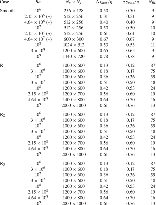
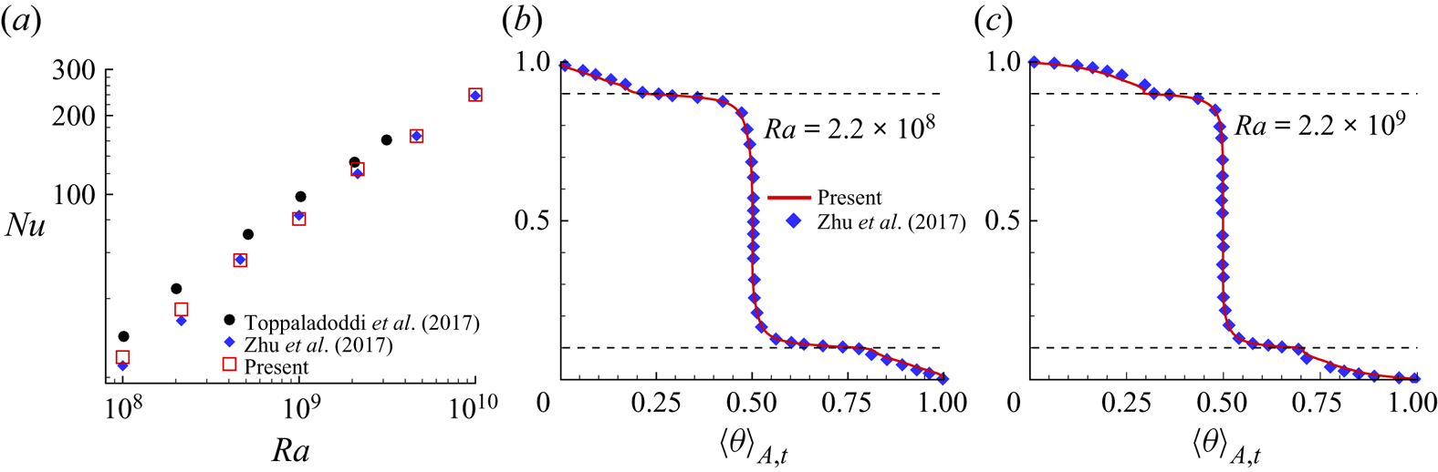
The governing equations are solved using a non-staggered finite volume method (Vishnu, De & Mishra Reference Vishnu, De and Mishra2019; Vishnu et al. Reference Vishnu, De and Mishra2020). To handle the irregular rough boundaries, the diffuse interface immersed boundary method is used (De Reference De2016, Reference De2018). The numerical set-up is validated extensively by reproducing the results of Zhu et al. (Reference Zhu, Stevens, Verzicco and Lohse2017) carried out in a sinusoidal rough geometry. The validation details are provided in § A.1. The flow is resolved up to the Kolmogorov length scale  $\eta =H\sqrt {Pr}\,Ra^{-1/4}\,(Nu-1)^{-1/4}$, which is ensured by
 $\Delta x_{max}/\eta <1$ and
 $\Delta y_{max}/\eta <1$; see table 1. Here,
 $\Delta x_{max}$ and
 $\Delta y_{max}$ are the maximum grid spacings in the
 $x$ and
 $y$ directions, respectively. Following the criterion given by Shishkina et al. (Reference Shishkina, Stevens, Grossmann and Lohse2010) to resolve the flow near the walls, a sufficient number of grid points are used inside the boundary layer. Simulation details of all the cases are listed in table 1. A grid independence test for four different grid spacings is carried out to select a suitable mesh for calculations; see § A.2. For converged statistics, sampling of at least
 $200$ free-fall time units is carried out in the statistically stationary state. Note that the conduction state (
 $\bar {u}=0$ and
 $\theta =1-y$) is used as the initial condition. Wang et al. (Reference Wang, Wan, Yan and Sun2019) reported that stability of the flow states is sensitive to the initial condition only at smaller inclinations (
 $<15^{\circ }$). Since the present work deals with greater tilts, we do not observe any dependence of flow states on initial conditions, which is consistent with Wang et al. (Reference Wang, Wan, Yan and Sun2019). However, it is observed that orientation of the flow states changes but does not influence the plume-emitting and -ejecting regions. To ascertain the effect of orientation on global heat transport, we compare the heat flux for different initial conditions at
 $Ra=10^{8}$, and observe a minimal change (less than
 $2\,\%$) in
 $Nu$ for R
 $_1$ and R
 $_3$ cases. In the simulated
 $Ra$ range, the statistical convergence of the
 $Nu$ data is confirmed by a maximum difference of
 $1.46\,\%$ in two equal successive sampling intervals. To resolve the rough boundaries, we use a highly refined mesh in the wall-normal direction, whose details are provided in § A.3. For the roughness cases,
 $Ra$ is calculated based upon the effective height of the cell as suggested by Zhu et al. (Reference Zhu, Stevens, Shishkina, Verzicco and Lohse2019). Note that the effective height is defined as the ratio of the volume occupied by fluid in the rough convection cell to the base area of the smooth case. The height (
 $h$) and wavelength (
 $\lambda$) of roughness elements are selected using the standard random number generator function with random seed in order to generate different sequences of numbers in different realizations. Since the finite axial length can accommodate a few finite roughness elements, no meaningful distribution function can be constructed for the roughness elements, owing to the lack of sample data. Thus, although we intend to show randomly varying roughness elements, their distribution can be best described as irregular. We have also shown the convergence of
 $Nu$ for different flow realizations using different roughness arrangements in § A.4. Note that the rough surfaces are generated by keeping nearly the same wetted area to neglect its effect for
 $Nu$ comparison.
Simulation details for the level case. From left to right: type of convection cell; Rayleigh number ( $Ra$); number of grid cells in the
 $x$ and
 $y$ directions (
 $N_x\times N_y$); ratio of maximum grid spacing to the Kolmogorov length scale
 $\eta =H\sqrt {Pr}\,Ra^{-1/4}\,(Nu-1)^{-1/4}$ in the
 $x$ (
 $\Delta x_{max}/\eta$) and
 $y$ (
 $\Delta y_{max}/\eta$) directions, respectively; number of points inside the thermal boundary layer (
 $N_{BL}$). Note that the reference Nusselt number for the smooth case is taken from Chand et al. (Reference Chand, Sharma, Venugopal and De2019), while for the roughness case, it is taken for the multi-scale roughness geometry in Zhu et al. (Reference Zhu, Stevens, Shishkina, Verzicco and Lohse2019). Here,
 $*$ refers to the
 $\phi =75^{\circ }$ cases only.

3. Results and discussions
In the current work, we first study the transformation of large-scale flow structures with inclination in the smooth case, followed by the effect of  $\phi$ on heat flux. Here, we identify the control parameters (
 $Ra$ and
 $\phi$) that yield maximum heat flux. The effect of tilt on turbulent intensity is studied further. Using three different roughness set-ups, we investigate the effect of rough boundaries and tilt on flow structures and global heat transport properties in §§ 3.4–3.6. We identify the
 $Ra$ range where IC effectively transports heat, and provide
 $Nu(Ra)$ and
 $Re(Ra)$ scaling laws for each inclination case.
3.1. Effect of inclination on flow structures
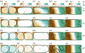
It is well-known that flow structures in RBC are sensitive to the inclination angle (Wang et al. Reference Wang, Xia, Wang, Sun, Zhou and Wan2018a) and aspect ratio (Wang et al. Reference Wang, Wan, Yan and Sun2018b). The sensitivity here refers to a change in the state of large-scale rolls. Figure 2 shows the instantaneous temperature fields for all five tilt angles and four  $Ra$ cases. The effect of the inclination angle is evident in all
 $Ra$ cases, where flow structures transform from a double-roll state at
 $\phi =0^{\circ }$ to a thermally stratified state at
 $\phi =90^{\circ }$. While the former is a consequence of a double aspect ratio, the thermal stratification occurs due to a temperature gradient acting normal to the gravity in the latter. These states have already been identified in previous studies (Shishkina Reference Shishkina2016; Shishkina & Horn Reference Shishkina and Horn2016; Khalilov et al. Reference Khalilov, Kolesnichenko, Pavlinov, Mamykin, Shestakov and Frick2018). Similar transformations of the flow states were observed by Wang et al. (Reference Wang, Xia, Wang, Sun, Zhou and Wan2018a) for the same governing parameters. However, for
 $\varGamma =1/2$, Wang et al. (Reference Wang, Wan, Yan and Sun2019) observed an unstable triple-roll state at smaller tilt angles (close to the level case), and a single-roll state beyond
 $\phi \approx 10^{\circ }$.
Instantaneous temperature field overlaid by streamlines showing the variation in large-scale rolls as the inclination angle increases from  $\phi =0^{\circ }$ to
 $\phi =90^{\circ }$. The
 $Ra$ values are (a–e)
 $10^{6}$, (f–j)
 $10^{7}$, (k–o)
 $10^{8}$, and (p–t)
 $10^{9}$. The
 $\phi$ values are (a,f,k,p)
 $0^{\circ }$, (b,g,l,q)
 $15^{\circ }$, (c,h,m,r),
 $45^{\circ }$ (d,i,n,s)
 $75^{\circ }$, and (e,j,o,t)
 $90^{\circ }$. The arrows in (a–e) indicate the direction of gravity. For any specific tilt angle except
 $\phi =0^{\circ }$, the flow states change with
 $Ra$.

At  $Ra=10^{6}$, it is observed that flow structures attain the shape of the cell at
 $\phi =15^{\circ }$ (see figure 2b), where the direction of thermal plumes is aligned such that hot plumes move rightwards along the hot isothermal wall, and cold plumes opposite to it. As a consequence, an LSC forms instead of a double-roll state. In the earlier studies, a large-scale roll is termed as LSC in a unit-aspect-ratio cell (Shishkina & Horn Reference Shishkina and Horn2016). Therefore, inclination incites LSC that spans the entire cell, which is consistent with Guo et al. (Reference Guo, Zhou, Qu, Cen and Lu2017), though the flow state changes with further increase in inclination angle. At
 $\phi =45^{\circ }$, movement of hot and cold fluid is restricted to the right and left parts of the cell, respectively, indicating weak thermal stratification with the central region showing fluid mixing. At
 $\phi =75^{\circ }$ and
 $90^{\circ }$, flow structures are nearly the same, and the flow becomes thermally stratified. Flow states at
 $Ra=10^{7}$ remain the same as for
 $Ra=10^{6}$, and this is also consistent with previous studies (Wang et al. Reference Wang, Xia, Wang, Sun, Zhou and Wan2018a). However, large-scale structures undergo significant changes beyond
 $Ra=10^{8}$; see figures 2(p–t), where these effects are more pronounced for
 $Ra=10^{9}$. It is clearly evident that a double-roll state persists even at
 $\phi =15^{\circ }$, and the organization of corner rolls is similar to that in the level case. At
 $\phi =45^{\circ }$, signatures of thermal stratification are absent, and sudden detachment of thermal plumes from the smooth walls is observed at randomly located spots. Unlike the level case, in a tilted set-up, thermal plumes (travelling along the isothermal surface) experience both buoyancy and induced shear. Therefore, it is quite apparent that both these forcings are competing with each other. While travelling along the hot surface, thermal plumes gain heat continuously. Once they attain sufficient energy to overcome the viscous resistance, they detach and move directly into the bulk, which impacts the heat flux to be described in § 3.2. The observed weak thermal stratification suggests that an increase in
 $Ra$ delays it, where the delay is in terms of inclination angle. This feature becomes more prominent for the highest
 $Ra$ case, where evidence of relatively higher fluid mixing is seen even at
 $\phi =75^{\circ }$. In this case, a complex flow state is observed, where several circulation cells are evident in relatively smaller regions of the cell, which restrict the movement of fluid. Notably, we find that the transition to a single large-scale circulation shifts towards a greater inclination angle as
 $Ra$ increases. This observation is in contrast to the results reported by Wang et al. (Reference Wang, Xia, Wang, Sun, Zhou and Wan2018a). They found that the above-mentioned shift first increases with inclination from
 $10^{7}$ to
 $5\times 10^{7}$, and eventually drops beyond
 $7\times 10^{7}$.
To ascertain the weakening of turbulence with increasing inclination, we show time series of vertical velocity fluctuations  $v^{\prime }$ obtained from a probe placed near the geometric centre of the cell,
 $x=1.1$,
 $y=0.5$, at
 $Ra=10^{7}$ and
 $10^{9}$ in figure 3. The vertical velocity is chosen because it signifies the rise of thermal plumes in the bulk region. At
 $Ra=10^{9}$, in the level case, large fluctuations are evident in figure 3(a). With increase in inclination angle, the fluctuations drop and nearly vanish at
 $\phi =90^{\circ }$. The sharp fluctuations signify movement of thermal plumes at the geometric centre. As shown in figures 3(c–e), a weak fluctuating signal in intermediate and higher tilt angles shows the absence of vertical movement of thermal plumes in the bulk region. It indicates movement of the flow along the walls, and the diminishing effect of buoyancy in the transverse direction is responsible for such movement. In comparison to
 $Ra=10^{7}$, evidence of fluctuations in vertical velocity at
 $Ra=10^{9}$ is seen clearly at
 $\phi =75^{\circ }$, which confirms better mixing of fluid relative to the lower
 $Ra$ case.
Time series of vertical velocity fluctuation  $v^{\prime }=v-\langle v \rangle _t$ in the vicinity of the geometric centre of the convection cell,
 $x=1.1$,
 $y=0.5$, for
 $Ra=10^{7}$ and
 $10^{9}$ at all five inclination angles. With increase in inclination angle, intensity of fluctuations drops in both the
 $Ra$ cases. Plots are for (a)
 $\phi = 0^{\circ }$, (b)
 $\phi = 15^{\circ }$, (c)
 $\phi = 45^{\circ }$, (d)
 $\phi = 75^{\circ }$, (e)
 $\phi = 90^{\circ }$.

3.2.  $Nu\unicode{x2013}\phi$ dependence

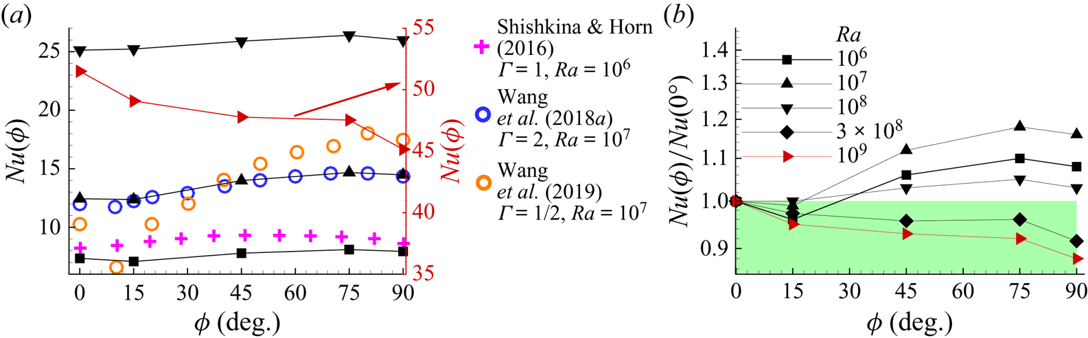
The Nusselt number from the present study is compared with a few previously reported data in figure 4(a). Our data agree well with Wang et al. (Reference Wang, Xia, Wang, Sun, Zhou and Wan2018a) for  $Ra=10^{7}$. A marginal difference is noted for
 $Ra=10^{6}$ with Shishkina & Horn (Reference Shishkina and Horn2016), who used
 $\varGamma =1$. At small to moderate
 $Ra$ (
 $\leq 10^{8}$), the
 $Nu(\phi )$ trend remains the same, while it drops monotonically for
 $Ra=10^{9}$, which is shown in a separate scale. To compare directly the
 $Nu\unicode{x2013}\phi$ dependence at different
 $Ra$ values, we show the normalized heat flux in figure 4(b). For
 $Ra \leq 10^{8}$, a drop in
 $Nu$ at
 $\phi =15^{\circ }$ is evident in all the cases. With further increase in
 $\phi$, it starts rising again to attain a maximum at
 $75^{\circ }$. Interestingly, the
 $Nu(\phi )$ trend becomes weaker with increasing
 $Ra$, and drops monotonically beyond
 $Ra>10^{8}$. In contrast to the present work, Wang et al. (Reference Wang, Wan, Yan and Sun2019) obtained a similar and robust
 $Nu(\phi )$ trend up to
 $Ra=10^{9}$ in the convection cell of
 $\varGamma =1/2$. This inconsistency can be attributed to the differences in the aspect ratio. For VC, the distance between the hot and cold plates in
 $\varGamma =1/2$ is twice of that in
 $\varGamma =2$, which favours thermal stratification and delays the onset of turbulence. Since greater tilt is effective in transporting heat due to laminar characteristics of the flow, Wang et al. (Reference Wang, Wan, Yan and Sun2019) did not observe any variation in the
 $Nu(\phi )$ trend due to the dominating thermal stratification. They attributed the minimum
 $Nu$ at smaller inclination angles to the double-roll state at
 $Ra=10^{6}$, and stable triple-roll state at
 $Ra=10^{7}$ and
 $10^{8}$. On the other hand, as seen in figures 2(b,g,l,q), we observe that flow exhibits a single-roll state in the two lower
 $Ra$ cases, and a double-roll state in the other two higher ones. Contrary to the previous studies where the single-roll state was found responsible for enhancing the heat flux (Wang et al. Reference Wang, Wan, Yan and Sun2019), we find the same state to diminish it for
 $Ra\leq 10^{7}$. This shows that the
 $Nu(\phi )$ dependence is similar for
 $\varGamma =1/2$ and
 $2$ at lower
 $Ra$ (
 $\leq 10^{8}$) despite different flow states.
(a) Comparison of  $Nu(\phi )$ curve obtained in the present work with Shishkina & Horn (Reference Shishkina and Horn2016) (
 $Ra=10^{6}$,
 $\varGamma =1$ and
 $Pr=1$), Wang et al. (Reference Wang, Xia, Wang, Sun, Zhou and Wan2018a) (
 $Ra=10^{7}$,
 $\varGamma =2$ and
 $Pr=0.71$), and Wang et al. (Reference Wang, Wan, Yan and Sun2019) (
 $Ra=10^{7}$,
 $\varGamma =1/2$ and
 $Pr=0.71$). Note that the arrow indicates the vertical axis (red) for the highest
 $Ra$ case. (b) Variation of normalized heat flux with inclination, where
 $Nu$ data are normalized by those of the level case
 $\phi =0^{\circ }$.

Next, we identify the inclination angles that yield maximum heat flux for each  $Ra$ case. It is evident that IC with greater tilt (
 $\phi =75^{\circ }$) transports heat most efficiently until
 $Ra=10^{8}$, where
 $\phi =75^{\circ }$ is seen as the optimum inclination angle. However, beyond
 $Ra=10^{8}$, RBC transports heat more efficiently. To observe the
 $Nu(Ra)$ trend for the optimum inclination angle, we further present the variation of normalized
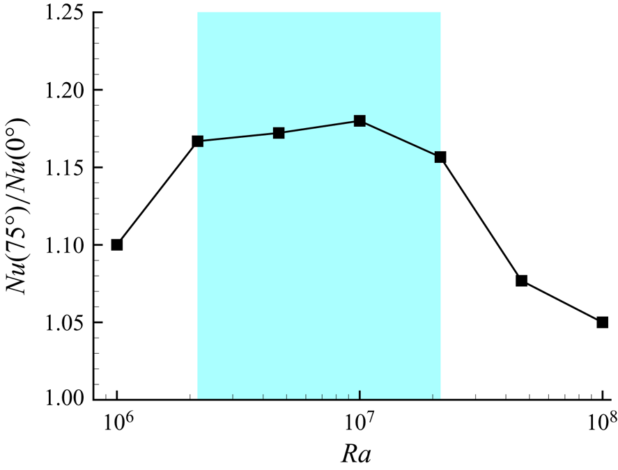
 $Nu$ by including four extra data points in figure 5. Heat flux initially rises with
 $Ra$ to become maximum at
 $Ra=10^{7}$, and drops monotonically beyond it. Interestingly, the optimum inclination becomes the most effective one at
 $Ra=10^{7}$, with an increment of
 $18\,\%$ in
 $Nu$. As shown by the shaded region, we observe a range
 $2.15\times 10^{6} \leq Ra \leq 2.15\times 10^{7}$ where increment in heat flux is more than
 $15.7\,\%$. Below and above this range, a sudden drop in augmented heat flux is noted.
Identification of the  $Ra$ range where IC transports heat in the most efficient manner for
 $\phi =75^{\circ }$. The shaded region represents the range
 $2.15\times 10^{6} \leq Ra \leq 2.15\times 10^{7}$ where significant increment in heat flux is obtained.

We further explore why the normalized heat flux drops with increasing  $Ra$ at
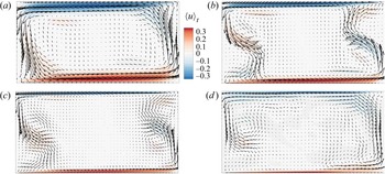
 $\phi =75^{\circ }$. To answer this question, we show the time-averaged velocity field in the direction of IS overlaid by velocity vectors in figure 6. It is noted that with increase in
 $Ra$, the intensity of the velocity drops near the isothermal walls. At the highest
 $Ra$, hot and cold fluid movement towards the opposite plates is obstructed due to the formation of several small-scale flow structures. These structures redirect the cold (hot) fluid towards the colder (hotter) region, and restrict the fluid mixing. In other words, weakening of thermal convection in the direction of IS is responsible for the reduced heat flux at higher
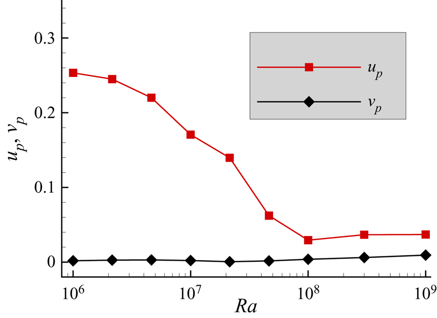
 $Ra$. In figure 7, we quantify the drop in the velocity near the hot plate. Here,
 $N=10$ equispaced probes are placed at distance
 $y/H=0.05$ to obtain the mean velocity in the direction of IS (
 $u_p$) and NIS (
 $v_p$), which are computed as
 \begin{gather} u_p=\frac{1}{N}\sum_{i=1}^{N}{|\langle u_i \rangle_{t}|}, \end{gather}
 \begin{gather} v_p=\frac{1}{N}\sum_{i=1}^{N}{|\langle v_i \rangle_{t}|}, \end{gather}
where  $i$ and
 $\langle \,{\cdot } \,\rangle _t$ represent the probe number and time average. Clearly,
 $u_p$ drops monotonically until
 $Ra=10^{8}$, and becomes nearly constant beyond it, which shows weak convection in the direction of IS. However,
 $v_p$ is insignificant compared to
 $u_p$, which is expected at such a greater tilt due to thermal stratification.
For  $\phi =75^{\circ }$, component of time-averaged velocity field in the direction of IS overlaid by velocity vector at
 $Ra$ values (a)
 $10^{6}$, (b)
 $10^{7}$, (c)
 $10^{8}$, and (d)
 $10^{9}$. With increase in
 $Ra$, the strength and region of velocity in the direction of IS diminish.

For  $\phi =75^{\circ }$, strength of velocity in the direction of the IS and NIS as a function of
 $Ra$. The velocities are computed from probes placed at distance
 $y/H=0.05$ units away from the hot plate.

One reason to consider the three decades of  $Ra$ in the present study is to establish a
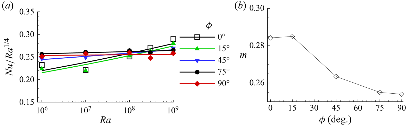
 $Nu(Ra)$ dependence for each inclination angle, which is described as follows. Figure 8(a) shows the compensated
 $Nu(Ra)$ scaling law in order to study the deviation from
 $Nu\sim Ra^{1/4}$. The greater tilt cases follow strictly the
 $1/4$ law, whereas a significant deviation is observed as
 $\phi$ approaches the level case. Further, in figure 8(b), we show the variation of the
 $Nu(Ra)$ scaling exponent
 $m$ with
 $\phi$ and find that a slight tilt does not alter the scaling exponent. On the other hand, it drops sharply as the cell is tilted beyond
 $\phi =15^{\circ }$. Evidently, the exponent becomes nearly invariant for
 $\phi \geq 75^{\circ }$. It is evident that
 $m$ is higher (
 $m=0.284$) in RBC than in VC (
 $m=0.254$), due to which the
 $Nu(\phi )$ curve shifts downwards with increasing
 $Ra$. Consequently, the most efficient heat transport state turns out to be the level case for
 $Ra >10^{8}$.
(a) The compensated Nusselt number showing the attainment of a  $1/4$ power law as inclination increases from
 $\phi =0^{\circ }$ to
 $\phi =90^{\circ }$. (b) Variation of the
 $Nu(Ra)$ scaling exponent with inclination angle.

3.3. $Re\unicode{x2013}\phi$ dependence

The Reynolds number ( $Re$) is another response parameter that depends upon
 $Ra$ and inclination. It is a measure of turbulent intensity and computed as
 $Re=\sqrt {Ra/Pr}\,U$, where
 $U=\sqrt {\langle \bar {u}\,\boldsymbol{\cdot}\,\bar {u}\rangle }$; see (2.4a,b). In figure 9(a), we show a comparison of absolute
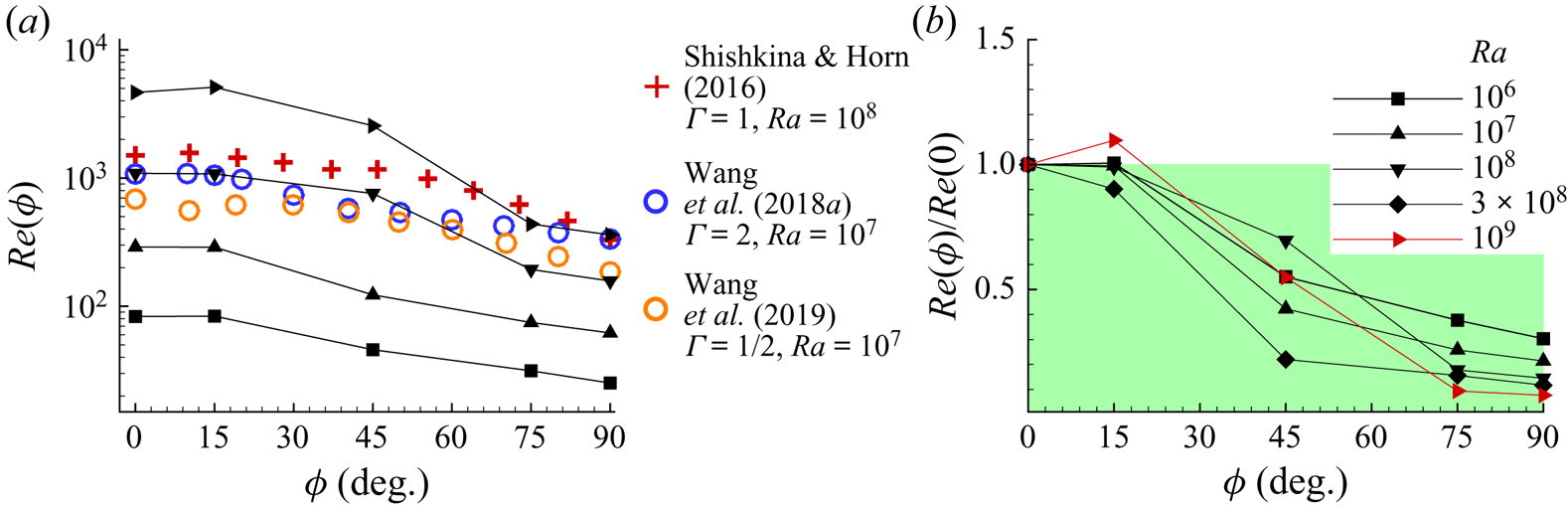
 $Re$ among the present study, Shishkina & Horn (Reference Shishkina and Horn2016) and Wang et al. (Reference Wang, Xia, Wang, Sun, Zhou and Wan2018a, Reference Wang, Wan, Yan and Sun2019). We observe that the trend of
 $Re$ in the present work agrees well with these studies. It is noted that with increasing
 $\phi$,
 $Re$ first remains nearly the same up to
 $\phi =15^{\circ }$, and then drops monotonically. For a direct comparison of
 $Re(\phi )$ at different
 $Ra$, we present the normalized
 $Re(\phi )/Re(0)$ data in figure 9(b), where the shaded region shows
 $Re<Re(0^{\circ })$. It is observed that
 $Re$ remains unaltered until
 $\phi =15^{\circ }$ for
 $Ra\leq 10^{8}$, whereas it increases by nearly
 $10\,\%$ in the highest simulated
 $Ra$ case. For
 $Ra=10^{9}$,
 $Nu(\phi )$ shows a reduction in heat flux for
 $\phi =15^{\circ }$, which is in contrast to the
 $Re$ value at the same inclination. Thus in a double-aspect-ratio configuration, despite unaltered or a small increase in turbulent intensity, the drop in
 $Nu$ indicates that the enhanced turbulent intensity does not necessarily improve the heat flux. A similar observation was made by Jiang et al. (Reference Jiang, Sun and Calzavarini2019), who reported that instead of turbulent intensity, the strength of LSC enhances
 $Nu$. However, the double-roll state at
 $\phi =15^{\circ }$ in figure 2(q) seems to be responsible for the enhanced turbulent intensity at
 $Ra=10^{9}$. With a further increase in inclination angle,
 $Re$ plummets sharply, and decreases by more than
 $90\,\%$ at
 $\phi =90^{\circ }$. The observed trend is different to what Wang et al. (Reference Wang, Wan, Yan and Sun2019) found, where
 $Re$ first drops and then rises again before following the monotonically decreasing trend. Again, this inconsistency may be attributed to the differences in the aspect ratio, which plays a significant role in determining the turbulent intensity due to the gap between the two isothermal walls. This analysis also suggests that
 $Re$ drops fastest in the intermediate inclination range and not near the vertical convection.
(a) Comparison of the  $Re(\phi )$ trend obtained in the present work with Shishkina & Horn (Reference Shishkina and Horn2016) (
 $Ra=10^{8}$,
 $\varGamma =1$ and
 $Pr=1$), Wang et al. (Reference Wang, Xia, Wang, Sun, Zhou and Wan2018a) (
 $Ra=10^{7}$,
 $\varGamma =2$ and
 $Pr=0.71$) and Wang et al. (Reference Wang, Wan, Yan and Sun2019) (
 $Ra=10^{7}$,
 $\varGamma =1/2$ and
 $Pr=0.71$). (b) Variation of normalized Reynolds number with inclination. Note that the normalization is carried out with respect to the level case (
 $\phi =0^{\circ }$). The shaded region highlights the drop in Reynolds number below the level case.

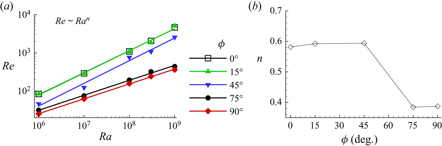
In figure 10, we show the least squares fit of  $Re(Ra)$ data. For
 $\phi =0^{\circ }$, we observe that
 $Re \sim Ra^{0.59}$, which is in good agreement with the previous studies (Sugiyama et al. Reference Sugiyama, Calzavarini, Grossmann and Lohse2009; Zhang et al. Reference Zhang, Zhou and Sun2017; Yang et al. Reference Yang, Wei, Zhu, Dou and Qian2018; Chand et al. Reference Chand, De and Mishra2021b). In addition, we further study the
 $Re(Ra)$ dependence for other inclination angles, which have not been reported so far. The level case
 $\phi =0^{\circ }$, and
 $\phi =15^{\circ }$, follow nearly the same power law,
 $Re \sim Ra^{0.59}$. In these two cases, the collapse of
 $Re(Ra)$ curves indicates the insignificant effect of a smaller inclination angle on turbulent intensity, which is also supported by the obtained flow states. With further increase in
 $\phi$ (
 $=45^{\circ }$), we observe the same scaling exponent but with a significant drop in absolute
 $Re$. The observed drop may be attributed to the single-roll state. In comparison to a double-roll state, thermal plumes, driven by a single roll, traverse a larger distance to reach the opposite plate. As a result, thermal plumes diffuse early, which diminishes the strength of the single large-scale roll. In the two highest
 $\phi$ cases, the
 $Re(Ra)$ values nearly follow the same power law and the least scaling exponent
 $n=0.39$. Figure 10(b) shows the variation of
 $n$ with
 $\phi$, where the exponent remains nearly the same until
 $\phi =45^{\circ }$, and subsequently drops to a significantly lower value for the two highest inclination cases. The variation in the exponent signifies differences in the transport mechanism. While the higher exponent marks the presence of turbulence in the flow, its lower counterpart highlights the signature of laminar characteristics, which can also be seen from the stratified temperature field in figure 2.
(a) Least squares fit of the  $Re(Ra)$ data for all the inclination angles. (b) Variation of the
 $Re(Ra)$ scaling exponent with inclination angle.

3.4. Effect of inclination on flow structures in the rough cells
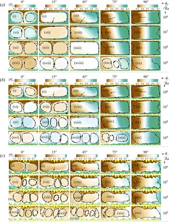
In figures 11(a–c), we present time-averaged temperature fields overlaid by streamlines for R $_1$, R
 $_2$, and R
 $_3$ configurations, respectively, to identify the changes in flow state with Rayleigh number and tilt angle. The temperature fields are shown for increasing
 $Ra$ and
 $\phi$. In the R
 $_1$ case, flow features change from a double-roll state in the level case to the stratified flow in the VC (
 $\phi =90^{\circ }$) for all
 $Ra$ cases, where only the central part of the cell shows a homogeneous mixing of hot and cold fluid. On the other hand, flow structures in the inclined cases
 $\phi =15^{\circ }$,
 $45^{\circ }$ and
 $75^{\circ }$ show transformation from the double-roll state to a single-roll state (except at
 $\phi =75^{\circ }$ for the highest
 $Ra$), spanning the entire cell. In the lowest
 $Ra$ case, the effect of inclination is significant as it brings the double–single roll state transformation at
 $\phi =15^{\circ }$ and incites thermal stratification at
 $\phi =45^{\circ }$. With increasing
 $Ra$, the effect of inclination becomes weaker as the flow structures appear to be the same at
 $\phi =0^{\circ }$ and
 $15^{\circ }$ for
 $Ra=10^{8}$. Since thermal plumes shrink with increasing
 $Ra$, smaller-sized plumes, owing to their greater mobility at higher
 $Ra$, do not align themselves in a single-roll state at
 $\phi =15^{\circ }$. Further, at
 $\phi =75^{\circ }$, with respect to the smooth case, a weaker thermal stratification and relatively better fluid mixing is evident in the cell. As
 $\phi$ approaches
 $90^{\circ }$, thermal stratification is seen clearly where nearly still, cold and hot fluids are present in the vicinity of the cold and hot isothermal walls of the cell, respectively.
For configurations (a) R $_1$, (b) R
 $_2$ and (c) R
 $_3$, time-averaged temperature fields superimposed with streamlines for
 $Ra=10^{6}$ (i–v),
 $10^{7}$ (vi–x),
 $10^{8}$ (xi–xv), and
 $10^{9}$ (xvi–xx). The inclination angle varies from left to right in the order:
 $\phi =0^{\circ }$,
 $15^{\circ }$,
 $45^{\circ }$,
 $75^{\circ }$ and
 $90^{\circ }$. The arrows in the first row of each roughness case indicate the direction of gravity.

In the intermediate roughness configuration (R $_2$), a large-scale roll is attained at
 $\phi =15^{\circ }$ for the lowest
 $Ra$ case. For
 $Ra=10^{7}$, we observe that the flow state remains the same for
 $\phi =0^{\circ }$ and
 $15^{\circ }$. Such a response of flow structures towards inclination is also observed in R
 $_1$, but at a higher
 $Ra=10^{8}$. For
 $Ra=10^{8}$, a triple-roll state is evident at
 $\phi =15^{\circ }$, while for the highest
 $Ra$ case, a triple-roll state is found for all the inclinations in the range
 $15^{\circ }\leq \phi \leq 75^{\circ }$. At
 $\phi =75^{\circ }$, it appears that thermal stratification has vanished due to the presence of a multiple-roll state. On the other hand, it is still evident in VC, although weaker.
Features of the flow structures that appeared in the R $_2$ case become more pronounced in the tallest roughness configuration (R
 $_3$), as shown in figure 11(c). The tendency of transformation of the flow state in the level case to higher tilt angles is found to be the same for the lower
 $Ra$ cases (up to
 $Ra=10^{7}$) in the R
 $_2$ and R
 $_3$ configurations. However, beyond
 $Ra=10^{7}$, significant differences are observed in the R
 $_3$ case. Increasing roughness height delays the emergence of a single large-scale roll that depends upon the inclination. In particular, this transition appears at
 $\phi =75^{\circ }$ and
 $90^{\circ }$ for
 $Ra=10^{8}$ and
 $10^{9}$, respectively. For the highest
 $Ra$, multiple smaller rolls persist at
 $\phi =45^{\circ }$ and
 $75^{\circ }$, respectively. As observed for the R
 $_2$ case, these rolls improve mixing of fluid in the cell. The most interesting feature appears in VC, where we observe that thermal stratification is nearly absent. It is evident that roughness delays thermal stratification due to its ability to break the large-scale rolls and emit thermal plumes directly into the bulk region. It can also be viewed as early onset of turbulence in greater tilt cases. Since increase in roughness height reduces the distance between isothermal walls, increase in turbulent intensity is obvious, which is reflected in delayed thermal stratification. This result elucidates why Wang et al. (Reference Wang, Wan, Yan and Sun2019) observed greater heat flux at greater inclination even at
 $Ra=10^{9}$.
3.5. Effect of inclination on $Nu$ in the presence of roughness

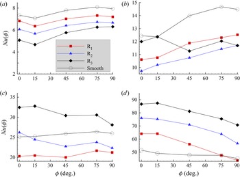
Figure 12 shows a comparison of  $Nu(\phi )/Nu(0^{\circ })$ among the smooth, R
 $_1$, R
 $_2$ and R
 $_3$ cases for the four
 $Ra$ values that cover the entire simulated
 $Ra$ range. For the lowest
 $Ra$, the
 $Nu(\phi )/Nu(0^{\circ })$ trend is same for all three roughness cases which is similar to the smooth case. It happens because of a weaker thermal forcing, due to which fluid remains inside the cavities (Zhang et al. Reference Zhang, Sun, Bao and Zhou2018; Chand et al. Reference Chand, Sharma and De2021a). Also, all the roughness elements are buried under a thick thermal boundary layer. The stagnant fluid and the thicker boundary layer suppress the effect of roughness at lower
 $Ra$, yielding a
 $Nu(\phi )$ trend similar to that of the smooth case. We observe that
 $Nu(\phi )$ drops until
 $\phi =15^{\circ }$, and rises with further increase in inclination angle. In the smooth, R
 $_1$ and R
 $_2$ cases, the maximum heat is transported at
 $\phi =75^{\circ }$. On the other hand, VC (
 $\phi =90^{\circ }$) yields maximum heat flux in R
 $_3$. For any particular tilt angle, heat flux decreases as the configuration changes from the smooth to the R
 $_3$ case. Since the cavity space increases from R
 $_1$ to R
 $_3$, the volume of stagnant fluid inside it also increases. In such a scenario, heat is transferred only through conduction. Therefore, for lower
 $Ra$, this study suggests that the taller the roughness height, the lower the heat flux, which answers why the smooth case yields the highest heat flux, and R
 $_3$ the least.
Dependence of heat flux on inclination angle for  $Ra$ values (a)
 $10^{6}$, (b)
 $10^{7}$, (c)
 $10^{8}$, and (d)
 $10^{9}$, in R
 $_1$, R
 $_2$ and R
 $_3$ configurations. The
 $Nu(\phi )$ curve does not change with roughness configurations at the lowest and highest
 $Ra$.

For  $Ra=10^{7}$ (see figure 12b), the normalized
 $Nu(\phi )$ curves in R
 $_1$ and R
 $_2$ are nearly similar except for
 $\phi =15^{\circ }$, whereas a completely different trend is observed for the R
 $_3$ case. Contrary to the smooth case,
 $Nu$ increases monotonically in the R
 $_1$ and R
 $_2$ cases, to become maximum at
 $90^{\circ }$. This suggests that small asperities on the isothermal walls make the vertical convection the most efficient heat transport system. In R
 $_3$,
 $Nu$ is either higher or comparable to R
 $_1$ and R
 $_2$. This happens because roughness elements in R
 $_3$ become active at this
 $Ra$ (
 $=10^{7}$) and perturb the thermal boundary layer to modify the flow structures by directly injecting thermal plumes in the bulk (Chand et al. Reference Chand, Sharma and De2021a). On the other hand, owing to their relatively shorter height with respect to the thermal boundary layer, roughness elements in the other two cases remain buried inside it. Here, active roughness refers to those elements that actively participate in emitting thermal plumes and are not buried inside the thermal boundary layer. The idea of activation is seen clearly from the nearly the same
 $Nu(\phi )$ trends in the two smaller roughness cases.
For  $Ra=10^{8}$, the trend in all three configurations reverses completely due to differences in active roughness peaks. In this case, flow states in R
 $_1$ and R
 $_2$ are the same beyond
 $\phi =15^{\circ }$, which is also reflected by a similar
 $Nu(\phi )$ trend in figure 12(c). On the other hand, in R
 $_3$, the trend becomes nearly the same beyond this
 $Ra$. This similarity is attributed to the early onset of transition to a multiple-roll state in R
 $_3$ through taller roughness peaks. Also, beyond this
 $Ra$, R
 $_3$ yields higher heat flux than the smooth, R
 $_1$ and R
 $_2$ cases. The reason for the highest heat flux in R
 $_3$ is again multiple rolls and boundary layer penetrating peaks. In Chand et al. (Reference Chand, Sharma and De2021a), it was already noted for the level case that onset of the enhanced heat flux regime occurs at
 $Ra=2.15\times 10^{8}$,
 $5.50\times 10^{7}$ and
 $10^{7}$ in the R
 $_1$, R
 $_2$ and R
 $_3$ cases, respectively, which supports the above arguments.
For the highest  $Ra$ (
 $=10^{9}$), maximum heat flux is produced by the tallest case (R
 $_3$), and the minimum by the smooth case. Interestingly, the trend of increasing heat flux with roughness heights at the lowest
 $Ra$ value reverses at the highest value. The reason behind this change is the presence of multiple rolls (five large-scale rolls) in R
 $_3$, whereas maxima of three and two rolls are present in the R
 $_2$ and R
 $_1$ cases, respectively. Basically, a larger number of rolls improves the plume ejection spots, which enhance
 $Nu$ (Wang et al. Reference Wang, Verzicco, Lohse and Shishkina2020). Another physical argument that can be made here is widening of the cavities with increasing roughness height. Wider cavities have a higher tendency to get washed out more efficiently to enhance the emission of thermal plumes (Toppaladoddi et al. Reference Toppaladoddi, Succi and Wettlaufer2017; Zhang et al. Reference Zhang, Sun, Bao and Zhou2018).
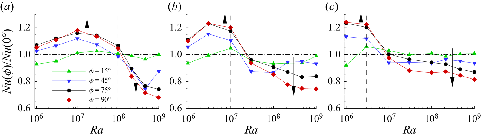
For each inclination angle, we further show the variation of normalized heat flux with  $Ra$ in figure 13. Based on
 $Nu/Nu(0)$, we define enhanced,
 $Nu>Nu(0)$, and reduced,
 $Nu<Nu(0)$, heat flux regimes. Note that the
 $Ra$ value beyond which the enhanced heat flux regime changes to the reduced one is termed the critical Rayleigh number (
 $Ra_c$). For the R
 $_1$, R
 $_2$ and R
 $_3$ cases,
 $Ra_c$ is found as
 $10^{8}$,
 $10^{7}$ and
 $3\times 10^{6}$, respectively. The width of the enhanced heat flux regime diminishes with increasing roughness height. In this regime,
 $Nu/Nu(0)$ increases with inclination, as shown by upward arrows. However, a contrasting effect of
 $\phi$, represented by the downward arrows, is seen in the reduced heat flux regime. The transition in the
 $Nu(\phi )$ trend reflects the onset of turbulence, which again supports our observation that RBC transports heat more efficiently than IC at larger
 $Ra$. From R
 $_1$ to R
 $_3$, the decrease in
 $Ra_c$ signifies early onset to turbulence due to a surge in plume emission (Chand et al. Reference Chand, De and Mishra2021b). In particular, we observe maximum improvements of
 $18\,\%$,
 $24\,\%$ and
 $25\,\%$ in heat flux for the R
 $_1$, R
 $_2$, and R
 $_3$ cases, respectively. On the other hand, following the same order, maximum reductions of
 $32\,\%$,
 $25\,\%$ and
 $17\,\%$ in heat flux are observed in the reduced heat flux regime.
Variation of the normalized heat flux  $Nu(\phi )/Nu(0)$ with
 $Ra$ for (a) R
 $_1$, (b) R
 $_2$, and (c) R
 $_3$ configurations at four different inclinations. While the vertical dashed line demarcates the enhanced and reduced heat flux regimes, the horizontal dash-dotted line represents
 $Nu(\phi )/Nu(0^{\circ })=1$. The upward (downward) arrows indicate increasing (decreasing)
 $Nu$ with
 $\phi$.

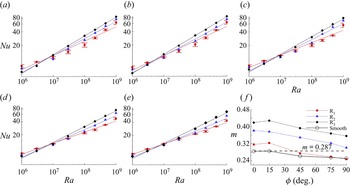
Next, we study the effect of tilt on  $Nu(Ra)$ dependence by showing the least squares fit of the
 $Nu$ data in figures 14(a–e), and
 $m(\phi )$ behaviour in figure 14(f). In the R
 $_1$ case, note that deviation from the fitting at the highest
 $Ra$ is observed up to
 $\phi =45^{\circ }$, which indicates the late onset of turbulence (higher
 $Ra_c$). The deviation is also evident from the rising error bar in figures 14(a–c). However, as
 $\phi >45^{\circ }$, the error bar nearly vanishes, which signifies the laminar heat transport throughout the simulated
 $Ra$ range. This is apparent from the similar
 $m(\phi )$ trend in R
 $_1$ and the smooth case beyond
 $\phi =45^{\circ }$. For these two cases, the exponent drops to
 $m\approx 1/4$ in VC, which is consistent with previous results (Churchill & Chu Reference Churchill and Chu1975; Shishkina Reference Shishkina2016). On the other hand, the early onset of turbulence is responsible for the higher exponent in the two taller roughness configurations. A direct connection between the turbulent intensity and scaling exponent is evident as the configuration changes from R
 $_1$ to R
 $_3$ in figure 14(f). It is interesting to note that despite significant differences in roughness heights, the
 $m(\phi )$ trend remains nearly the same in the three cases. Here, the effect of decreasing
 $m(\phi )$ corresponds to the drop in heat flux as
 $Ra$ increases beyond
 $Ra_c$.
Least-squares fits of  $Nu(Ra)$ at different inclination angles: (a)
 $\phi =0^{\circ }$, (b)
 $\phi =15^{\circ }$, (c)
 $\phi =45^{\circ }$, (d)
 $\phi =75^{\circ }$, (e)
 $\phi =90^{\circ }$. (f) The
 $Nu(Ra)$ scaling exponent
 $m$ as a function of inclination angle for the R
 $_1$, R
 $_2$ and R
 $_3$ cases. The dashed line in the last frame represents
 $m=0.287$ obtained for the smooth case at
 $\phi =0^{\circ }$. Note that the
 $Nu(Ra)$ data are presented with error bars in the R
 $_1$ case to show deviation from the least squares fit.

3.6. Effect of inclination on $Re$ in the presence of roughness

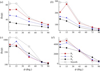
Figure 15 shows the variation of Reynolds number with inclination at four  $Ra$ values that cover the entire simulated
 $Ra$ range. Similar to the smooth case, the
 $Re(\phi )$ curve shows a consistent trend where it remains nearly identical or changes slightly at small inclination (
 $\phi =15^{\circ }$), and drops monotonically with further increase in
 $\phi$ in all four
 $Ra$ cases. However, roughness impacts the turbulent intensity, which is reflected in the deviation from the smooth case in
 $Re(\phi )$. At lower
 $Ra$ (
 $\leq 10^{7}$), roughness height suppresses the turbulent intensity, i.e. the taller the roughness height, the lower the turbulent intensity. This happens due to the stagnant fluid residing in the cavities at lower
 $Ra$. It is also reflected from the nearly the same
 $Re$ values in the smooth and R
 $_1$ cases, where the flow structures are similar. Beyond
 $Ra=10^{8}$, as expected, differences in
 $Re$ in the three configurations reduce due to movement of fluid in the cavities (secondary vortices), which washes them out. The role of roughness heights is remarkable for a greater tilt at
 $Ra=10^{9}$. Here, while
 $Re$ between
 $\phi =75^{\circ }$ and
 $90^{\circ }$ changes marginally in the smooth case, a significant difference is evident as the roughness configuration changes from R
 $_1$ to R
 $_3$. This indicates clearly weaker thermal stratification and greater mixing of fluid at these two inclinations in taller roughness configurations, as observed in the flow structures in § 3.4. Contrary to lower
 $Ra$ cases, we observe that the
 $Re(\phi )$ trend does not show notable changes until
 $\phi =45^{\circ }$ for the highest
 $Ra$. This can be attributed to the similar flow structures that show a greater turbulent intensity at this inclination range for
 $Ra=10^{9}$. On the other hand, evidence of thermally stratified flow at
 $\phi =45^{\circ }$ for lower
 $Ra$ cases is responsible for the sudden drop in
 $Re$.
 $Re\unicode{x2013}\phi$ dependence for three roughness cases and the smooth case at four
 $Ra$ values: (a)
 $10^{6}$, (b)
 $10^{7}$, (c)
 $10^{8}$, and (d)
 $10^{9}$. The
 $Re\unicode{x2013}\phi$ curves in the roughness cases are similar to the smooth case. Note that while
 $Re$ decreases from R
 $_1$ to R
 $_3$ at lower
 $Ra$, it becomes comparable in all three configurations at the highest
 $Ra$.

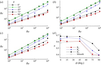
We study further the effect of inclination on  $Re(Ra)$ dependence for different inclination angles in figure 16. The least squares fit of
 $Re(Ra)$ data clearly shows that the scaling laws
 $Re\sim Ra^{n}$ for
 $\phi =0^{\circ }$ and
 $15^{\circ }$ are nearly the same, where the scaling exponents for R
 $_1$, R
 $_2$ and R
 $_3$ are
 $0.61$,
 $0.64$ and
 $0.68$, respectively. The nearly the same exponents for the
 $\phi =0^{\circ }$ and
 $15^{\circ }$ cases indicates a similar transport mechanism, which is also reflected in their flow structures. Note the effect of roughness on the scaling exponent, which is nearly same for the smooth and tiny roughness heights. However, as roughness changes from R
 $_1$ to R
 $_3$, the exponent increases with respect to the smooth case. For
 $\phi =45^{\circ }$, although turbulent intensity decreases, the scaling exponent remains nearly the same as in the two smaller inclinations, which is reflected by the
 $n(\phi )$ trend in figure 16(d). However, beyond
 $\phi =45^{\circ }$, the exponent as well as turbulent intensity drops remarkably due to settling down of the cold and hot fluid near the the cold and hot walls of the cell, respectively (see the time-averaged temperature field in figure 11). For
 $\phi =75^{\circ }$ and
 $90^{\circ }$, we observe that the exponent in the smooth and R
 $_1$ cases does not change appreciably, which indicates a similar flow state. On the other hand, flow structures in R
 $_2$ and R
 $_3$ change significantly at these inclinations, which is also reflected in their
 $n(\phi )$ trend. In R
 $_3$, greater turbulent intensity (weaker thermal stratification) as compared to the other smaller roughness set-ups at
 $\phi =75^{\circ }$ is responsible for a higher scaling exponent.
For five inclinations, least squares fits of  $Re$ data for (a) R
 $_1$, (b) R
 $_2$, and (c) R
 $_3$. (d) The
 $n\unicode{x2013}\phi$ trend for the three roughness cases and the smooth case. The scaling exponent remains nearly the same until
 $\phi =45^{\circ }$, and drops beyond this range.

4. Summary and conclusions
We have investigated the effect of inclination on heat flux in a wide range of  $Ra$ values varying from
 $10^{6}$ to
 $10^{9}$ in two-dimensional tilted RBC. The present work is carried out in a double-aspect-ratio convection cell filled with air (
 $Pr=0.71$) for five inclination angles (
 $\phi =0^{\circ },15^{\circ },45^{\circ },75^{\circ },90^{\circ }$) for both rough and smooth cases. Shishkina & Horn (Reference Shishkina and Horn2016) suggests that
 $Nu(\phi )$ and
 $Re(\phi )$ trends are non-monotonic complex functions of
 $Ra$ and
 $Pr$. In the same line, the present work has addressed one of these complexities, i.e. the effect of
 $Ra$ on
 $Nu(\phi )$ dependence for a relatively wider cell (
 $\varGamma =2$) in two-dimensional RBC. We have listed the
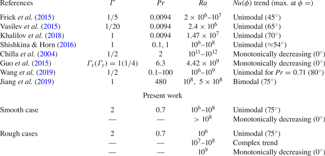
 $Nu(\phi )$ trend observed in the previous studies and current work in table 2. Based upon the analysis, we have made the following observations.
(i) In the smooth case, inclined convection can be used to enhance the heat flux below
$Ra=10^{8}$, whereas above it, RBC yields the highest heat flux. On the other hand, for the roughness cases, effectiveness of IC (determined by $Ra_c$) to transport heat shifts to lower $Ra$ as the characteristic height of the roughness increases due to early onset of turbulence.(ii) In the smooth case, the maximum heat flux is obtained at
$\phi =75^{\circ }$ for $Ra \leq 10^{8}$, while for the roughness cases, it depends upon the $Ra$ and roughness set-ups.(iii) For
$\phi =75^{\circ }$, in the smooth case, a range $2.15\times 10^{6} \leq Ra \leq 2.15\times 10^{7}$ is identified wherein heat flux improves significantly, at least by $15\,\%$. In the three roughness configurations, we observed increments of $18\,\%$, $24\,\%$ and $25\,\%$ in $Nu$ for the R$_1$, R$_2$ and R$_3$ cases, respectively.(iv) For both smooth and roughness cases, with increase in
$Ra$, transition to a single large-scale circulation shifts towards a greater tilt angle. Moreover, an increase in roughness height also delays this transition. Contrary to the previous observations (Wang et al. Reference Wang, Wan, Yan and Sun2019), a single-roll state is found to diminish heat flux for $Ra \leq 10^{7}$ at $\phi =15^{\circ }$.(v) While increase in
$Ra$ delays the onset of thermal stratification in the smooth case, increase in the characteristic height of the roughness set-ups does the same in rough configurations, which indicates early onset of turbulence in greater tilt cases.(vi) Similar to the effect of
$Ra$ on $Nu(\phi )$ dependence, the $Re(\phi )$ trend remains nearly the same up to $Ra=10^{8}$, and changes marginally beyond this. It is also found that $Re$ drops faster in the intermediate inclination range than near the VC.


Summary of  $Nu(\phi )$ trend in inclined thermal convection. From left to right: references; aspect ratio (
 $\varGamma$); Prandtl number (
 $Pr$); Rayleigh number (
 $Ra$); the characteristic of the
 $Nu(\phi )$ trend; and the inclination angle at which maximum heat flux is obtained. Here, unimodal and bimodal in
 $Nu(\phi )$ trend refer to single and dual peaks, respectively.

Funding
This work is funded by SERB through project no. CRG/2019/000177. All the simulations were carried out in Param-Ishan, a 250-teraflops supercomputing facility at IITG.
Declaration of interests
The authors report no conflict of interest.
Appendix A. Details of the numerical set-up
In what follows, we first show the validation of the numerical set-up followed by the effectiveness of the solver to handle the rough surfaces. Further, details of the grid independence test are provided, and finally, the effect of different flow realizations on  $Nu$ is shown. Note that the level case (
 $\phi =0^{\circ }$) is chosen for all these studies.
A.1. Validation of the numerical set-up
The correctness of the current numerical set-up is established by reproducing the results reported by Zhu et al. (Reference Zhu, Stevens, Verzicco and Lohse2017). They used a uniform sinusoidal roughness geometry, whose amplitude ( $h=0.1$) and wavelength (
 $\lambda =0.1$) are
 $10\,\%$ of the height of the convection cell. We compare the
 $Nu$ and mean temperature profiles with their data, as shown in figure 17. The maximum and average difference of
 $7\,\%$ and
 $3\,\%$, respectively, in
 $Nu$ show the accuracy of the present numerical set-up. Moreover, overlapping of the time-averaged vertical temperature profiles at two different
 $Ra$ values also ensures the agreement of the set-up.
Comparison of (a)  $Nu(Ra)$ and (b,c) time-averaged vertical temperature profiles between the present, Zhu et al. (Reference Zhu, Stevens, Verzicco and Lohse2017) and Toppaladoddi et al. (Reference Toppaladoddi, Succi and Wettlaufer2017) data for sinusoidal roughness geometry. The horizontal dashed lines denote height of the roughness geometry.

A.2. Grid independence test
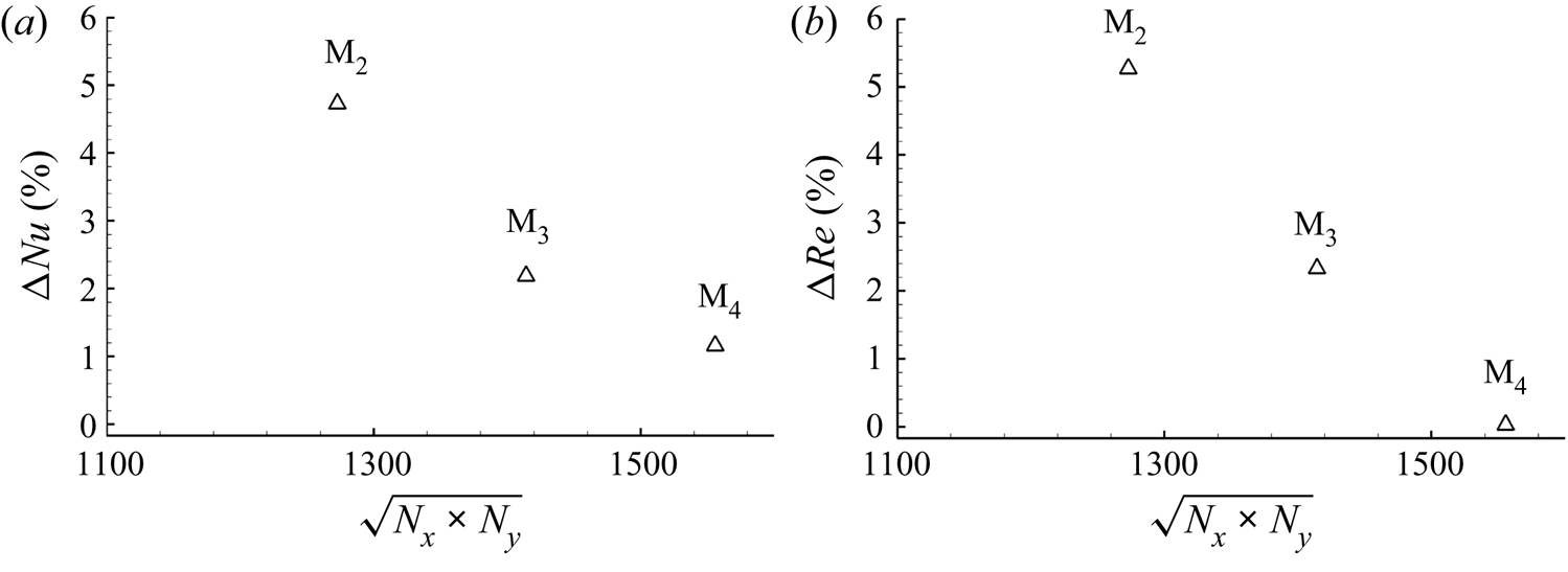
A grid independence test is conducted by progressively refining the mesh from the coarsest (M $_1$) to the finest (M
 $_4$) mesh. In this study, we have chosen the highest
 $Ra=10^{9}$ and observed the variation of
 $Nu$ and
 $Re$ with M
 $_i$ as shown in figure 18. As the mesh is refined from M
 $_1$ to M
 $_4$, the changes in the Nusselt number,
 $(Nu_i-Nu_{i-1})/Nu_{i-1}$, and the Reynolds number,
 $(Re_i-Re_{i-1})/Re_{i-1}$, decrease and become marginal beyond M
 $_3$. Thus M
 $_3$ is chosen as a reference grid for all subsequent calculations.
Change in the global (a)  $Nu$ and (b)
 $Re$ values at
 $Ra=10^{9}$ obtained by progressively refining the mesh (M
 $_i$,
 $i=1,2,3,4$). Note that the difference at a mesh (
 $i$) is computed using values at the previous (
 $i-1$) one.

A.3. Diffuse interface immersed boundary method
To handle the rough surface, we have used the diffuse interface immersed boundary method (DIIBM). This method categorizes computational cells into fluid, solid and interfacial cells. They are identified by the volume fraction ( $\phi =V_s/V_p$) criterion, which is defined as the ratio of volume of the body (
 $V_s$) present inside a cell to the entire computational cell (
 $V_p$). Note that for fluid, solid and interfacial cells,
 $\phi =0$,
 $\phi =1$ and
 $0<\phi <1$, respectively. The body surface can be reconstructed whose volume is calculated by
 \begin{equation} \sum_{cell} \phi_i V_{pi} = V_{body}, \end{equation}
and this is represented by the zero-level set function. Through the volume fraction, the equation of conservation of momentum and the motion of a rigid body are combined to construct a global equation, which is solved in the entire domain. Boundary conditions are not imposed directly but enforced through the global equation. Note that the scope of the boundary condition is limited to a computational cell. Thus for reasonably well-resolved simulations, results are nearly identical to the sharp interface method. For more details, refer to De (Reference De2018)
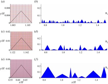
Accuracy of the rendered volume is the key in the reconstruction of body surfaces, which depends upon the mesh size. Therefore, a sufficiently refined mesh in the wall-normal direction is employed to resolve the roughness adequately. In figure 19, for the three roughness cases, we show the grid resolution of the smallest roughness element and the zero-level set representation of a part of the linearized rough surface. Note that we have shown the smallest roughness element at the smallest  $Ra=10^{6}$ because mesh refinement at higher
 $Ra$ further improves the body resolution. The presence of sufficient grid points inside the roughness elements, and nearly the exact representation of the rendered zero-level set function, confirm the body resolution. The rendered volume of the object yields an error of
 $0.08\,\%$ and
 $0.01\,\%$ for
 $Ra=10^{6}$ and
 $10^{9}$, respectively. The present numerical set-up was used previously for solving both stationary (De & Sarkar Reference De and Sarkar2020, Reference De and Sarkar2021a,Reference De and Sarkarb; Chand et al. Reference Chand, Sharma and De2021a,Reference Chand, De and Mishrab; Sharma, Chand & De Reference Sharma, Chand and De2022) and moving (Kushwaha & De Reference Kushwaha and De2020) boundary problems. For further details about the DIIBM, refer to De (Reference De2016, Reference De2018).
For the smallest  $Ra=10^{6}$, (a,c,e) representation of mesh overlaid by linearized smallest roughness element, and (b,d,f) the zero-level set representation of a part of the linearized rough surfaces in R
 $_1$, R
 $_2$ and R
 $_3$ configurations. The roughness elements are shown in a zoomed view for better visualization.

A.4. Different flow realizations
This subsection shows the convergence of  $Nu$ for different flow realizations obtained in different roughness geometries. Geometric characteristics (height and wavelength) of these cases vary in the range
 $0.005\leq h/H\leq 0.05$ (
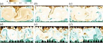
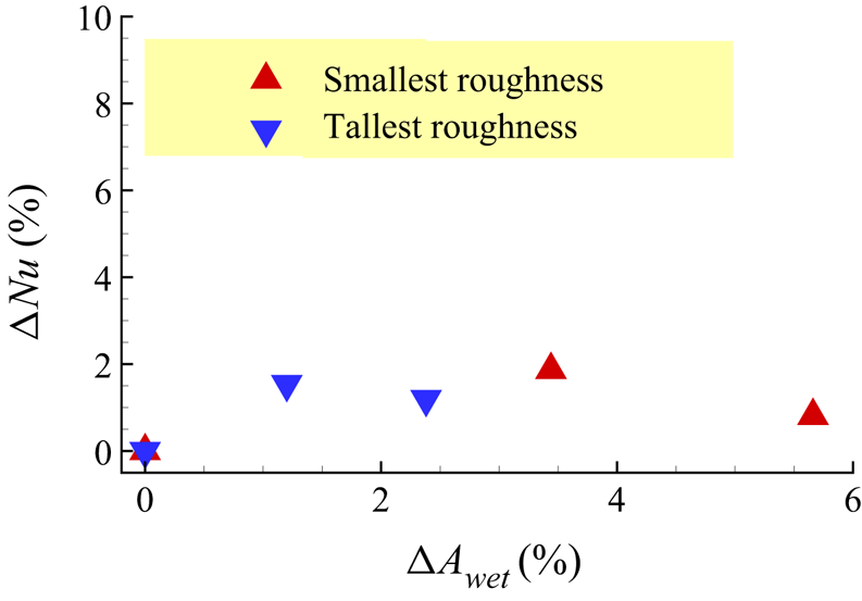
 $0.02\leq h/H\leq 0.2$) for the smallest (tallest) roughness case. In figure 20, the instantaneous temperature field in three different realizations shows distinct flow structures. However, heat flux remains nearly the same for the comparable wetted area, as shown in the figure 21. We have calculated the changes in heat flux (
 $\Delta Nu$) and wetted area (
 $\Delta A_{wet}$) with respect to the first realization of both the smallest and tallest roughness cases. It is observed that the maximum variation in
 $Nu$ (
 $A_{wet}$) remains less than
 $2\,\%$ (
 $6\,\%$), which is sufficiently small to show the independence of heat flux from the distribution of roughness height and wavelength.
Instantaneous temperature field in different flow realizations for (a–c) the smallest and (d–f) the tallest roughness set-ups. The roughness boundaries are different, but the range of variation of their height and wavelength is the same as that of the R $_1$ and R
 $_3$ cases.

Variation of change (with respect to the first realization) in  $Nu$ with wetted area (
 $\Delta A_{wet}$) of different flow realizations shown in figure 20. The filled red triangle and inverted blue one represent the smallest and tallest roughness geometries, respectively.