


1. Introduction
Rayleigh–Bénard (RB) convection, the flow in a layer heated from below and cooled from above, is a canonical model for the problem of thermal convection (Ahlers, Grossmann & Lohse Reference Ahlers, Grossmann and Lohse2009; Lohse & Xia Reference Lohse and Xia2010; Chillà & Schumacher Reference Chillà and Schumacher2012). The study of RB convection has proven so fruitful because the system is well-defined and closed and possesses non-trivial conservation properties accessible to theory and experiment, such as the exact relationship between kinetic energy dissipation and heat transport (Shraiman & Siggia Reference Shraiman and Siggia1990). However, most real systems, both in process technology and in nature, differ from the idealized RB set-up. Many modifications of the canonical system are possible, such as the addition of roughness (Tisserand et al. Reference Tisserand, Creyssels, Gasteuil, Pabiou, Gibert, Castating and Chilla2011; Rusaouën et al. Reference Rusaouën, Liot, Castaing, Salort and Chillà2018), finite conductivity effects on the plates (Verzicco Reference Verzicco2004; Brown et al. Reference Brown, Funfschilling, Nikolaenko and Ahlers2005) or different sidewall conditions (Xia & Lui Reference Xia and Lui1997; van der Poel et al. Reference van der Poel, Ostilla-Mónico, Verzicco and Lohse2014). A variation which has attracted recent attention is that of inhomogeneous temperature boundary conditions, which is of interest in geophysics (Pekeris Reference Pekeris1935; Solomatov & Moresi Reference Solomatov and Moresi2000; Lenardic & Moresi Reference Lenardic and Moresi2003; Lenardic et al. Reference Lenardic, Moresi, Jellinek and Manga2005). To model the difference between continental and oceanic lithospheres, studies have substituted the constant-temperature top boundary condition by a pattern of adiabatic and conducting boundary conditions, meant to represent the physical properties of continents and oceans, respectively (Cooper, Moresi & Lenardic Reference Cooper, Moresi and Lenardic2013; Ripesi et al. Reference Ripesi, Biferale, Sbragaglia and Wirth2014; Wang, Huang & Xia Reference Wang, Huang and Xia2017; Bakhuis et al. Reference Bakhuis, Ostilla-Mónico, Van Der Poel, Verzicco and Lohse2018). However, the experimental and numerical results for this configuration appear to be at odds with each other (Ostilla-Mónico Reference Ostilla-Mónico2017).
Studies of RB with mixed-temperature boundary conditions were pioneered by the simulations of Cooper et al. (Reference Cooper, Moresi and Lenardic2013), who studied the effect of large or small patches of adiabatic ‘continents’ in a doubly periodic, large-aspect-ratio RB simulation domain (cell). Cooper et al. (Reference Cooper, Moresi and Lenardic2013) found that the heat transfer was largely unaffected by the number of continental blocks, and depended on area coverage. These results were corroborated experimentally by Wang et al. (Reference Wang, Huang and Xia2017), who found that the heat transfer in their rectangular RB cell depended mainly on the conducting area, and was largely independent of the arrangement of the plates. For both studies, the arrangement of the plates had a substantial effect on the underlying flow. The role of plate size and shape was postulated to be crucial in understanding the role continental and oceanic plates play in the configuration of the mantle circulation, and how these interactions determine the dynamics of the Wilson cycle (Ostilla-Mónico Reference Ostilla-Mónico2017).
Conversely, the simulations of Ripesi et al. (Reference Ripesi, Biferale, Sbragaglia and Wirth2014) in two dimensions, and their recent extension by Bakhuis et al. (Reference Bakhuis, Ostilla-Mónico, Van Der Poel, Verzicco and Lohse2018) to three dimensions, focused on patches which have characteristic dimensions smaller than the distance between the plates. These simulations found that the arrangement of the plates, quantified as a stripe wavelength, had a substantial effect on the total heat transport, and that once the stripe wavelength became comparable to the size of the thermal boundary layer, the heat transport asymptotically reached the values corresponding to a fully conducting plate, even if the conducting area was only one-half. But unlike the studies mentioned above, both of these studies found that plate size had no significant effect on the flow dynamics.
The discrepancy between these two results becomes less apparent when one compares the wavelengths of the inhomogeneities. The stripes in the first case scenario, by Cooper et al. (Reference Cooper, Moresi and Lenardic2013) and Wang et al. (Reference Wang, Huang and Xia2017), are much larger than the stripes in the second case scenario, by Ripesi et al. (Reference Ripesi, Biferale, Sbragaglia and Wirth2014) and Bakhuis et al. (Reference Bakhuis, Ostilla-Mónico, Van Der Poel, Verzicco and Lohse2018). This discrepancy just indicates that there are two distinct regimes, and that a crossover between the two regimes must exist: between large adiabatic patches which significantly affect the flow topology and small adiabatic patches whose effect is only present very close to the plates, there must be a transitional regime with ‘medium-sized’ patches which affect both types of statistics. Because land masses such as continents and islands come in a wide variety of shapes and length-scales, understanding how these sizes and shapes affect the circulation of the mantle can enhance our understanding of continental drift.
In this study we set out to find the location and characteristics of the crossover regime between the ‘large’ and ‘small’ pattern behaviour, and to explore its characteristics through three-dimensional direct numerical simulations. For this, we will simulate three-dimensional RB with non-uniform temperature boundary conditions on the top surface, which are a mixture of adiabatic and perfectly conducting. We note that this transition might not happen at the same stripe size for different statistics, as has been seen for example in the transition between different flow regimes in rotating RB convection (Kunnen et al. Reference Kunnen, Ostilla-Mónico, van der Poel, Verzicco and Lohse2016).
2. Numerical details
We perform large-aspect-ratio simulations of RB flow using a second-order, centred finite difference code (van der Poel et al. Reference van der Poel, Ostilla-Monico, Donners and Verzicco2015). The code is periodic in the wall-parallel directions with equal periodicity lengths of  $L_x=L_y=L$. We fix the Rayleigh number to
 $Ra=g\beta {\rm \Delta} H^3/(\nu \kappa )=10^8$, and vary the Prandtl number
 $Pr=\nu /\kappa$ between
 $1$ and
 $100$, where
 $g$ is the acceleration of gravity,
 $\beta$ is the fluid thermal expansion coefficient,
 $\Delta$ is the hot-cold temperature difference,
 $H$ is the height of the cell, and
 $\nu$ and
 $\kappa$ are the kinematic viscosity and thermal diffusivity of the fluid. The temperature boundary conditions are imposed as Dirichlet boundary conditions on the conducting parts of the plates: the bottom plate is fixed to a temperature
 $\Delta$ above that of the conducting regions of the top plate. In this way, the Rayleigh number
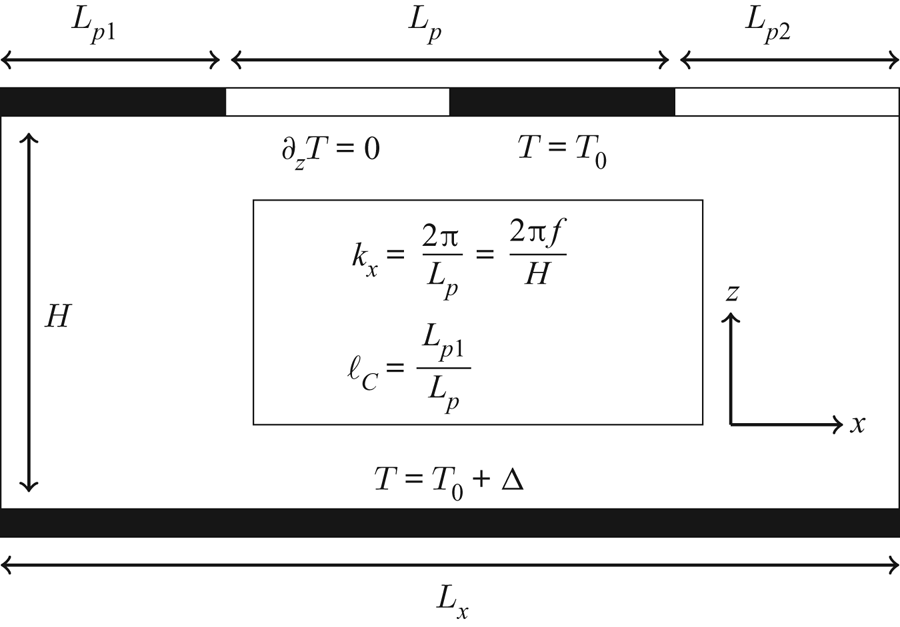
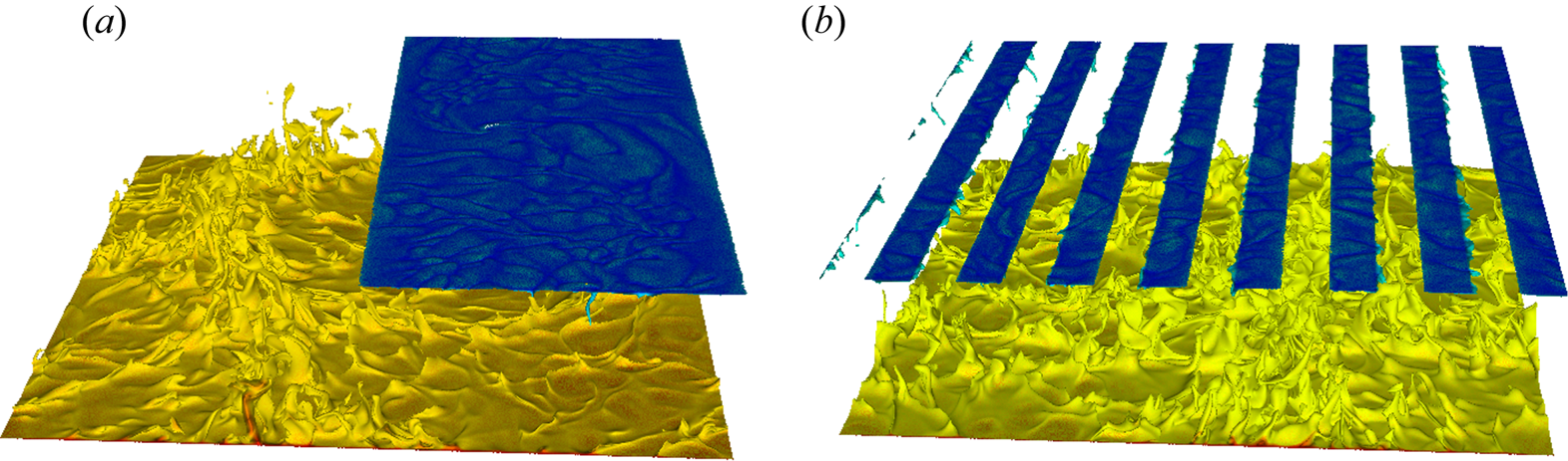
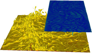
 $Ra$ can be thought of as a non-dimensional measure of the temperature difference while the Prandtl number is a fluid property. The two-dimensional adiabatic stripes are introduced in the top plate using Neumann no-flux conditions. This means that the temperature of the fluid close to the adiabatic plates is not determined a priori. See figure 1 for a sketch of the configuration and figure 2 for a flow visualization.
Schematic of the simulation set-up. The third dimension is removed for clarity purposes. The bottom plate is set at a constant (hot) temperature, while in the top plate, stripes of adiabatic and conducting boundary conditions alternate every  $L_p$. We set
 $L_{p1}=L_{p2}$ so that the effective area of conducting material is
 $50\,\%$.

Volume rendering visualization of the instantaneous temperature for two cases simulated at  $Ra=10^8$,
 $Pr=1$ and
 $\varGamma =4$. Red denotes hot fluid while blue denotes cold fluid. (a) Large stripes with
 $f=0.25$. The stripes cause a substantial ordering of the plume dynamics in the bottom plate, and an overall increase in temperature. (b) Small stripes with
 $f=2$. The stripes do not affect the flow dynamics at the bottom plate.

The non-dimensionalized periodicity of the system,  $\varGamma =L/H$, is a numerical parameter whose influence we want to remove as much as possible. We simulate aspect ratios in the range from
 $\varGamma =L/H=1$ to
 $\varGamma =16$. Previous studies (Stevens et al. Reference Stevens, Blass, Zhu, Verzicco and Lohse2018) have shown that it has a strong influence on the underlying statistics of the flow. As we will discuss further below, an adequately normalized heat transfer, as studied by Bakhuis et al. (Reference Bakhuis, Ostilla-Mónico, Van Der Poel, Verzicco and Lohse2018), does not show significant box-size/domain-size dependence. The temperature statistics show some box-size dependence, especially when the number of unit patterns in the domain is small. The velocity statistics show a strong box-size dependence, which increases with Prandtl number. For
 $Pr=1$, the velocity statistics for the two horizontal directions are approximately equal when
 $\varGamma \gtrsim 2$. But for
 $Pr=100$, even at
 $\varGamma =8$ we could not recover isotropic statistics in both horizontal directions. Therefore, velocity statistics will only be shown for
 $Pr=1$, where we can be sure that any anisotropy between the horizontal directions is produced by the inhomogeneous boundary conditions instead of by numerical effects.
To fully capture the crossover regime, we simulate a wide range of stripe wavenumbers  $k_x=2{\rm \pi} /L_p$, where
 $L_p=H/f$ is the stripe wavelength, and
 $f$ is the number of stripes per unit non-dimensional length (non-dimensionalized using the height). We set
 $L_{p1}=L_{p2}$, and keep the top plate equally partitioned between conducting and adiabatic regions. The largest wavelength covered is
 $f=1/8$, representing a single stripe pair in a
 $\varGamma =8$ domain. This wavelength is larger than that in the experiments by Wang et al. (Reference Wang, Huang and Xia2017), and will cover the full experimental parameter regime. The smallest wavelength is
 $f=90$, well into the asymptotic small-patch region according to Bakhuis et al. (Reference Bakhuis, Ostilla-Mónico, Van Der Poel, Verzicco and Lohse2018). Due to the second-order scheme of the code used, each stripe must be resolved by at least four points; otherwise artefacts are introduced. This means that to keep on increasing
 $\,f$, we would have to increase the resolution. Because of this, we limited ourselves to
 $f\leq 90$. Furthermore, we note that for some values of
 $f$, we have simulated several periodicity aspect ratios
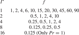
 $\varGamma$ to quantify the domain independence. A full list of all the simulated
 $\varGamma$ and
 $f$ is available in table 1.
Simulated values of  $f$ and
 $\varGamma$.

We will focus on one-dimensional stripes on the plates, as our previous exploration of chequerboard patterns showed that they do not produce significantly different physics (Bakhuis et al. Reference Bakhuis, Ostilla-Mónico, Van Der Poel, Verzicco and Lohse2018). However, stripes introduce an asymmetry between the two horizontal directions which can affect the flow enhancement. We have also simulated two cases with chequerboard inhomogeneities to better quantify the effects of boundary asymmetry against large, but isotropic, inhomogeneities.
The grid resolution used for this study conforms to the grid convergence study performed by Bakhuis et al. (Reference Bakhuis, Ostilla-Mónico, Van Der Poel, Verzicco and Lohse2018) for  $Pr=1$. For larger Prandtl numbers, we use the same resolution, and check its adequacy by monitoring the balance between viscous dissipation and heat transport outlined in Stevens, Verzicco & Lohse (Reference Stevens, Verzicco and Lohse2010). Finally, temporal convergence is assessed through measuring the non-dimensional heat transport, i.e. the Nusselt number
 $Nu=Q/(\kappa {\rm \Delta} H^{-1})$, with
 $Q$ the plate-to-plate heat transfer. While
 $Q$ can be measured in many ways (Shraiman & Siggia Reference Shraiman and Siggia1990), we use the volumetrically and temporally averaged value of
 $\langle u_z \theta \rangle$ to obtain the numerical value of
 $Q$. As this is a second-order correlation, which takes longer to converge, it provides some bounds on our temporal convergence errors. We have run the simulations for small domains with
 $\varGamma =1$ up to
 $1200$ large-eddy turnover times, and for larger domains with
 $\varGamma =8$ up to
 $120$ large-eddy turnover times. This gives us an error bound on temporal convergence of less than
 $1\,\%$.
3. Results
We start by showing a visualization of the instantaneous temperature field for two cases with different values of  $f$ in figure 2. From a cursory glance, we can confirm what was detailed in the introduction: two very different regimes exist, one where the stripes are small and the flow dynamics is not significantly affected as compared to the case of a fully conducting top plate (shown on the right), and one where the stripes are large and the flow dynamics is substantially changed due to the presence of a large adiabatic surface on only one side (shown on the left). The rest of this manuscript will involve teasing out the differences between the two flow regimes, when the transition between them happens, and how these differences affect the flow statistics.
3.1. Heat transfer
We first focus on the heat transfer, non-dimensionalized as a Nusselt number  $Nu$. The first step is to eliminate box-size dependence
 $\varGamma$, so that
 $Nu(\,f)$ can be properly elucidated. As mentioned previously, we have conducted simulations for different aspect ratios
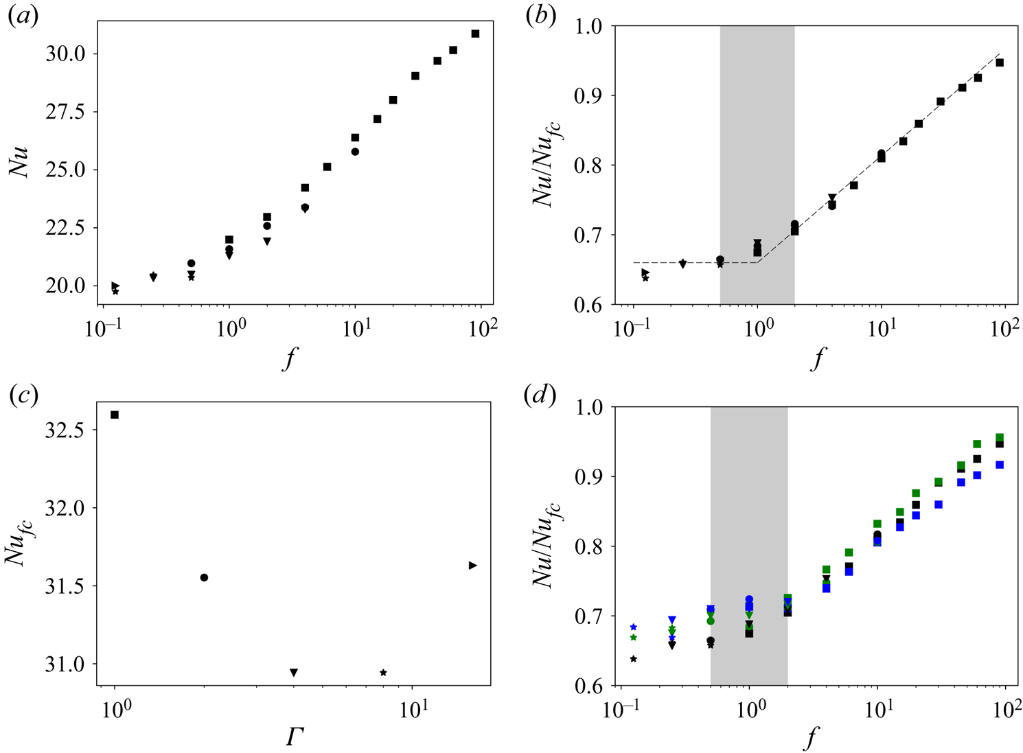
 $\varGamma$ with all other control parameters constant, to quantify as far as possible this dependence. Figure 3(a) shows the Nusselt number
 $Nu(\varGamma ,f)$ against stripe frequency for
 $Pr=1$. The box-size dependence of
 $Nu$ can be appreciated in the fact that the data points for the same values of
 $f$ do not fall onto each other when
 $\varGamma$ is changed. This is not surprising, because from RB simulations with homogeneous boundary conditions, it is known that for
 $Pr=1$, the Nusselt number shows some box-size dependence if
 $\varGamma \le 4$ (Stevens et al. Reference Stevens, Blass, Zhu, Verzicco and Lohse2018). This dependence is further quantified in panel (d), where the Nusselt number of the fully conducting (unmodified) system is shown as a function of
 $\varGamma$. While the variations are not very large, of the order of
 $6\,\%$, they are enough to introduce discrepancies into the measurements.
(a) Nusselt number against stripe number for  $Ra=10^8$ and
 $Pr=1$. A large variation between different values of
 $\varGamma$ can be seen. (c) Nusselt number variation as a function of box size for
 $Pr=1$. (b) Normalized Nusselt number for
 $Pr=1$. The box-size dependence is removed when normalizing by a
 $\varGamma$-dependent fully conducting
 $Nu_{fc}$. (d) Nusselt number normalized by the fully conducting value for each value of
 $\varGamma$. A large degree of collapse can be found across
 $Pr$. Symbols: colour denotes Prandtl number;
 $Pr=1$ is black,
 $Pr=10$ is green and
 $Pr=100$ is blue. Shape denotes
 $\varGamma$; squares are
 $\varGamma =1$, circles are
 $\varGamma =2$, V-triangles are
 $\varGamma =4$, stars are
 $\varGamma =8$ and
 $>$-triangles are
 $\varGamma =16$.

The  $\varGamma$ dependence can be removed by adequately compensating
 $Nu$. In figure 3(b), we plot the normalized Nusselt number
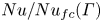 $Nu/Nu_{fc}(\varGamma )$, where
 $Nu_{fc}(\varGamma )$ is the Nusselt number for the homogeneous (fully conducting plates) case from the panel (c). With this operation, we get an excellent collapse across all box sizes, removing the
 $\varGamma$ dependence and elucidating the dependence on
 $f$. For values of
 $f$ less than
 $1$, the heat transport is almost constant, and independent of stripe wavelength. This is consistent with the observations by Cooper et al. (Reference Cooper, Moresi and Lenardic2013) and Wang et al. (Reference Wang, Huang and Xia2017). For values of
 $f$ greater than
 $1$, the heat transport begins to significantly increase, and tends towards the fully conducting value, which is consistent with Bakhuis et al. (Reference Bakhuis, Ostilla-Mónico, Van Der Poel, Verzicco and Lohse2018).
For our simulations we are not able to reach 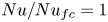 $Nu/Nu_{fc}=1$ because we are limited in the values of
 $f$ we can simulate. This asymptotic value for
 $Nu/Nu_{fc}$ was reached in Bakhuis et al. (Reference Bakhuis, Ostilla-Mónico, Van Der Poel, Verzicco and Lohse2018) at lower Rayleigh numbers. For this to happen, the pattern size has to be much smaller than the thermal boundary layer size, implying notably finer grid resolution. If we estimate the thermal boundary layer size as
 $\lambda _T/H=1/(2Nu)$, this gives us the requirement of
 $f\gg 2Nu$ for
 $Nu/Nu_{fc}\to 1$. With our current Rayleigh number
 $Ra=10^8$, this should happen for
 $f\gg 65$. The largest value of
 $f$ simulated,
 $f=90$, is insufficient to see this.
In figure 3(b), we also shade in a postulated transitional region  $0.5<f<2$ between the two regimes. None of the aforementioned studies examined values on both sides of
 $f=1$, i.e. they did not explore the transitional region between the two behaviours, so they unsurprisingly reached different conclusions on the behaviour of the heat transport.
We attempt to extend this result for all Prandtl numbers simulated in figure 3(d), which shows the normalized Nusselt number for three different Prandtl numbers. While the basic result remains, i.e. there is a sharp transition between two regimes of heat transport, the behaviour on both regimes appears slightly different. At first glance, the low-wavelength limit values of  $Nu/Nu_{fc}$ are higher with increasing
 $Pr$, but it remains to be seen if these values would continue dropping as
 $f$ decreases, or if this is a product of the increased box-size dependence seen for larger Prandtl numbers (Stevens et al. Reference Stevens, Blass, Zhu, Verzicco and Lohse2018). The slope of the
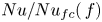 $Nu/Nu_{fc}(\,f)$ relationship also appears to be steeper for higher
 $Pr$. The mechanisms for this are unclear, and any speculation on these trends is out of the scope of this study. What appears to be a general conclusion is that the wide-stripe and thin-stripe regimes exist independently of
 $Pr$ in our range of
 $1\le Pr \le 100$, and we expect them to persist as the geophysically relevant regime
 $Pr\to \infty$ is entered.
3.2. Temperature profiles
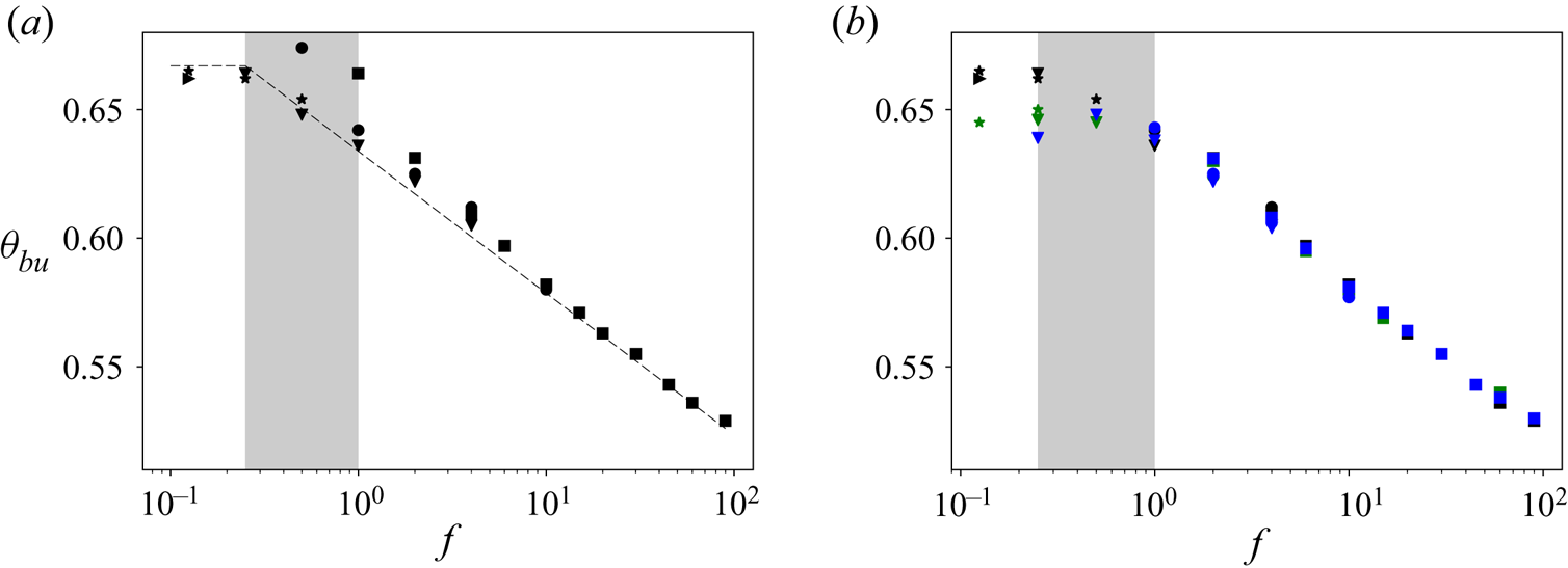
The next thing we study is the dependence of the mean temperature at the mid-plane on the value of  $f$. We do this by averaging the temperature in both horizontal directions, and in time (after the flow becomes statistically stationary). Bakhuis et al. (Reference Bakhuis, Ostilla-Mónico, Van Der Poel, Verzicco and Lohse2018) concluded that as
 $f\to \infty$, the temperature in the mid-plane region would tend towards the arithmetic mean of the temperatures of the two plates, i.e.
 $\theta =0.5$, and that as the stripes became larger
 $(\,f \to 0)$, the mean temperature would tend towards
 $2/3$. This was rationalized by taking an average of the temperatures at the two plates, weighted by the fraction of the plate which actually conducted heat. For
 $\ell _C=0.5$, this gives
 $\theta =2/3$.
Figure 4(a) shows the average mid-gap temperature as a function of  $f$ for
 $Pr=1$. In analysing the current simulations, it becomes clear that the simulations of Bakhuis et al. (Reference Bakhuis, Ostilla-Mónico, Van Der Poel, Verzicco and Lohse2018) have significant box-size dependence in their temperature measurements, due to the enforced periodicity constraining the flow and the development of large-scale structures. There is a strong box-size dependence in the transitional region. When running a small periodic box with only one or two stripes per simulation period, the temperature tends to increase due to the finite domain size. Only when
 $\varGamma =4$ or
 $\varGamma =8$ are these effects mitigated, and we can obtain box-size-independent results for
 $f\le 1$. As rationalized earlier, the mid-gap temperature can be seen to saturate to
 $\theta _{bu}=2/3$ for
 $f\le 0.25$, representing stripes of very large size. Consistent with Bakhuis et al. (Reference Bakhuis, Ostilla-Mónico, Van Der Poel, Verzicco and Lohse2018), we see a sharp temperature drop as
 $f$ increases beyond
 $f=1$. We have shaded in a transitional region, which now happens for other values of
 $f$:
 $0.25<f<1$. To adequately capture this region, simulations of
 $\varGamma \ge 4$ are needed, which were not performed in Bakhuis et al. (Reference Bakhuis, Ostilla-Mónico, Van Der Poel, Verzicco and Lohse2018).
(a) Mid-gap temperature as a function of  $f$ for
 $Pr=1$ and all box sizes simulated. The box-size dependence of some simulations is emphasized. (b) Mid-gap temperature as a function of
 $f$ for all
 $Pr$ simulated and selected box sizes. A clear transition between a constant-temperature region and a region of decreasing bulk-temperature can be seen. Shapes and colours of symbols are the same as in figure 3.

In figure 4(b) we show the bulk temperature as a function of  $f$ for all the Prandtl numbers explored. Simulations which have a single unit pattern per box size are taken out of the results. By doing this, we see how the curves collapse in the high-
 $f$ region. Again, there is a transitional region which happens for
 $0.25<f<1$. The values of
 $f$ at which this transition happens are independent of
 $Pr$, but are different from (smaller than) those from the transition we saw in
 $Nu/Nu_{fc}$. Because of this, the low-
 $f$ region appears decreased in size in the figure.
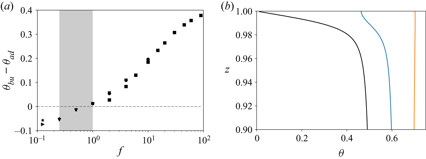
We can further explore the temperature statistics by analysing the behaviour of the average fluid temperature close to the adiabatic plates ( $\theta _{ad}$). Naively, we can expect the temperature of the adiabatic regions to tend towards the (cold) plate temperature
 $\theta =0$ as
 $f$ increases, and this is indeed what happens. What is more interesting is to look at the temperature difference between bulk and adiabatic region as a function of
 $\,f$, which we show in figure 5(a). For large
 $f$, the bulk is hotter than the adiabatic regions at the top, cold plate, as expected. However, for
 $f<1$, the fluid close to the adiabatic regions becomes slightly hotter than the bulk fluid (as well as the conducting parts of the same plate), which means that there is a slight temperature inversion. This provides another statistic that shows a change in behaviour during the transition.
(a) Difference between the mid-gap temperature  $\theta _{bu}$ and the average temperature of the fluid near the adiabatic plate as a function of
 $f$ for
 $Pr=1$ and all box sizes simulated. Shapes of symbols are the same as in figure 3. (b) Thermal boundary layer profiles close to the adiabatic plates for
 $\varGamma =4$,
 $Pr=1$ and
 $f=4$ (blue),
 $f=0.25$ (orange), and the reference (homogeneous) case (black).

To further understand what is happening, we show the thermal boundary layer close to the adiabatic regions for a small- $f$ and a large-
 $f$ case in figure 5(b). For large
 $f$, we can see that inside the boundary layer, there is a temperature increase, which means that there is horizontal transport of heat to the conducting regions. For small
 $f$, this gradient is not seen, which means that the horizontal transport of heat within the boundary layers is severely weakened. This has the potential to generate strong horizontal flows due to strong density gradients, which we analyse in the next section.
3.3. Velocity statistics and flow structure
Finally, we analyse the velocity statistics and the changes in flow structure. As mentioned in the introduction, from the experimental and numerical results we expect that the large-stripe cases show a strong effect on the wind, while the small-stripe cases should not be very different from the canonical set-up. We could also expect to see a strong asymmetry in the winds once the stripes pass a certain size, as excess heat must be redistributed horizontally from the zones close to adiabatic boundary conditions to the cooling parts of the plate.
To study the velocity statistics, we define the ‘wind’ Reynolds number in the  $i$th direction as
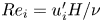 $Re_i=u^\prime _i H/\nu$, where
 $u^\prime$ is the volume-averaged root-mean-square velocity. We also define the horizontal wind Reynolds number as
 $Re_h=\sqrt {Re_x^2+Re_y^2}$. For the homogeneous case,
 $u_x^\prime$ should be equal to
 $u_y^\prime$, meaning
 $Re_x=Re_y$. This means that
 $Re_h$ should be equal to
 $\sqrt {2}Re_x$, which is also equal to
 $\sqrt {2}Re_y$. However, because of the restrictions present due to the finite domain (i.e. finite
 $\varGamma$),
 $Re_x$ and
 $Re_y$ often differ from each other. Of all the statistics presented in this manuscript,
 $Re$ has the largest box-size dependence. This is true even for the case of fully conducting plates, as was shown by Stevens et al. (Reference Stevens, Blass, Zhu, Verzicco and Lohse2018). For
 $Pr=1$,
 $Re_x$ and
 $Re_y$ differ from each other by about
 $5\,\%$, which gives us an estimate of the error made when measuring these quantities. For
 $Pr=10$ and
 $Pr=100$, the anisotropy is stronger, and causes deviations between
 $Re_x$ and
 $Re_y$ of over
 $100\,\%$. This means our error bars become too large to extract any meaningful information. Because of this, in this section we only show results for
 $Pr=1$.
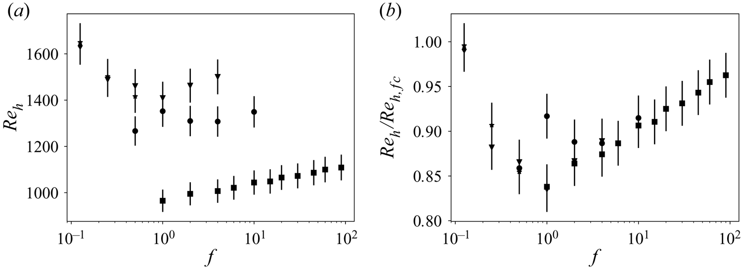
In figure 6(a), we show the horizontal Reynolds number  $Re_h$ as a function of
 $f$ for the different values of
 $\varGamma$. The dependence of
 $Re_h$ on
 $\varGamma$ is very strong: when comparing the values of
 $Re_h$ for the
 $f=10$ case at
 $\varGamma =1$ against the same
 $f$ at
 $\varGamma =2$,
 $Re_h$ can be seen to be as much as twice as large for
 $\varGamma =2$. When looking at both horizontal directions together, the underlying flow appears weaker than in the homogeneous case. This is further quantified in panel (b), where we show
 $Re_h$ normalized by the fully conducting value
 $Re_{h,fc}$, which is
 $\varGamma$-dependent. From the figure we can observe a local minimum for
 $Re_h$ around
 $f=1$. As
 $f\to \infty$, we recover the homogeneous
 $Re_h$, and as
 $f$ becomes smaller than unity, the wind is enhanced by strong horizontal temperature gradients. For no cases simulated does the total wind strength exceed that of the homogeneous flow even if the data hint that this will happen for
 $f<0.1$.
(a) Total horizontal flow strength quantified as a Reynolds number. (b) Total horizontal flow strength normalized by the homogeneous case. Symbol shapes are as in figure 3. Error bars of  $5\,\%$ are included on both plots.

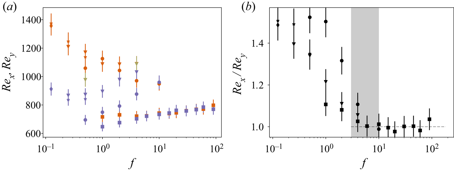
We now turn to the behaviour of the individual  $Re_i$ as a function of the stripe wavelength, which is illustrated in figure 7; here we expect to see differences between the
 $x$ and
 $y$ directions due to the asymmetry introduced by the stripes. In figure 7(a), we show the large variability between the different values of
 $Re_x$ and
 $Re_y$ for different box sizes and different values of
 $f$. We can highlight two trends. First, for large stripes (
 $f<1$), the wind in the direction normal to the stripes, i.e. the
 $x$ direction, is much larger than the wind in the direction parallel to the stripes, i.e. the
 $y$ direction. As the stripes become smaller, the winds tend to equalize. In the direction parallel to the stripes, the wind increases, while in the direction perpendicular to the stripes, the wind decreases. This is further quantified in figure 7(b), which shows the ratio between
 $Re_x$ and
 $Re_y$. Once the stripes are small enough, around
 $f=4$, the two Reynolds numbers become approximately equal, but they still are somewhat lower than the value for fully conducting plates, which is not reached until
 $f$ becomes much higher.
(a) Flow strength quantified as a Reynolds number in the stripe-normal ( $Re_x$, orange symbols) and stripe-parallel (
 $Re_y$, purple symbols) directions. Data for the average horizontal Reynolds number
 $([Re_x+Re_y]/2)$ for the chequerboard pattern simulations are included in khaki. (b) Ratio between the wind Reynolds numbers in the horizontal directions. Symbol shapes are as in figure 3. Error bars of
 $5\,\%$ are included on both plots. Only data for
 $Pr=1$ are presented here.

This asymmetric wind increase appears regardless of box size, even if there is some scatter on the magnitude of the asymmetry depending on  $\varGamma$. Again, we have highlighted the transitional region where the asymmetry disappears, which now occurs for higher values of
 $f$:
 $3<f<8$. We emphasize that the transitional ranges for the three statistics happen for different values of
 $f$, even if they are generally around
 $f=1$.
We have also simulated two cases with a chequerboard pattern. This pattern restores the  $x$–
 $y$ asymmetry, and serves to quantify how much of the wind enhancement comes from the necessity of transporting heat to the regions where it can be cooled by the plates instead of from the asymmetry of the system. The chequerboard cases were run for
 $\varGamma =4$ with
 $f=0.5$ and
 $f=4$. Unsurprisingly, we find that
 $Re_x\approx Re_y$ to within
 $5\,\%$, the previously reported error bound. What is more interesting is to compare the flow strength to the other case. This shows that the wind enhancement disappears with the flow asymmetry: for
 $f=0.5$ the value of the horizontal Reynolds number is lower than that for
 $f=16$, and this one is slightly below that of the homogeneous case. It is only when there is a strong asymmetry in the horizontal directions that intense large-scale flow patterns are generated in the direction perpendicular to the stripes, and the wind can exceed the value of the homogeneous case in a single direction.
As discussed in § 2 we only include results for  $Pr=1$. For
 $Pr=10$ and
 $Pr=100$, a similar enhancement of the flow strength and anisotropy could be seen when applying the stripe pattern, but we cannot confidently attribute it to physical reasons alone. For this reason we decided not to show these data. Further studies at increasing box size at high
 $Pr$ are required to adequately disentangle the box-size effects from those coming from inhomogeneous boundary conditions.
4. Conclusions
We have conducted numerical simulations of adiabatic–conducting stripe pairs of RB flow in an attempt to uncover the differences between the large-stripe regime of Cooper et al. (Reference Cooper, Moresi and Lenardic2013) and Wang et al. (Reference Wang, Huang and Xia2017) and the small-stripe regime of Ripesi et al. (Reference Ripesi, Biferale, Sbragaglia and Wirth2014) and Bakhuis et al. (Reference Bakhuis, Ostilla-Mónico, Van Der Poel, Verzicco and Lohse2018). We observed that for  $Ra=10^8$ and
 $Pr>1$, a transition between the two behaviours happens at around
 $f=1$, that is, with stripes the size of the plate distance. We note that the statistics show transitions at different values of
 $f$, and that these transitions can only be fully uncovered once the simulation ‘box size’ is large enough, but as a rule of thumb, they happen around
 $f\approx 1$. While this is not totally satisfactory, we point out that for rotating RB, we have previously seen that different statistics, such as fluctuations or mean temperature profiles, have different transition points (Kunnen et al. Reference Kunnen, Ostilla-Mónico, van der Poel, Verzicco and Lohse2016).
The small-stripe regime is characterized by a heat transport that is very dependent on stripe wavelength. With decreasing stripe wavelength, the bulk temperature and heat transport asymptotically tend to the fully conducting values, even when only half the plate is conducting. This regime was already explored in detail by Bakhuis et al. (Reference Bakhuis, Ostilla-Mónico, Van Der Poel, Verzicco and Lohse2018). Only when the stripes become very small, i.e.  $f\gg 2Nu$, do the statistics converge to those of fully conducting plates.
The large-stripe regime is characterized by a heat transport and a bulk temperature that is independent of stripe wavelength. To maintain the heat transport as the stripes become large, the underlying flow is heavily modified (as observed by Wang et al. Reference Wang, Huang and Xia2017) and the velocities in the stripe-normal direction increase substantially with increasing stripe length. The temperature stabilizes at values around  $2/3$, i.e. the weighted average of the plate temperatures, but this appears to depend on Prandtl number. There appears to be a local temperature inversion, where the temperature at the adiabatic plates is higher than the bulk temperature. This regime is geophysically interesting, as many variations on the RB problem, such as mantle convection, consist of very long wavelength inhomogeneities. We confirm here that these types of variations can lead to the enhancement of underlying ‘winds’ or circulations.
However, the conclusions here are limited in two main ways. The simulation of large- $Pr$ flows is complicated due to the resolution requirements and the computational box sizes. The effect of
 $Pr$ on enhancing winds has to be quantified in a more detailed manner. In the second place, the value of
 $l_C$, i.e. the ratio of conducting to adiabatic areas, has been fixed at one-half. Repeating this study for other values of
 $l_C$ is necessary to achieve more robust conclusions.
Acknowledgements
We thank A. Blass, D. Bakhuis and R. J. A. M. Stevens for providing their data. We thank the HPE Data Science Institute (HPE DSI) at the University of Houston for providing computing resources.
Declaration of interests
The authors report no conflict of interest.