2. Observational constraints on the evolution of massive stars: status quo

The simplest observational constraints on stellar evolution models are provided by counts of stars in different evolutionary phases, which can be performed in different galactic environments to trace the effects of initial chemical composition (metallicity) on the models. For the resolved stellar populations of the Local Group galaxies, one can determine, for example, the Wolf-Rayet (WR) to O-star ratio or the ratio of WC/WN subtypes of WR stars (see e.g. the discussion by Meynet & Maeder Reference Meynet and Maeder2005), or the blue supergiant (BSG) to red supergiant (RSG) ratio $B/R$ (Eggenberger et al. 2002), which is very sensitive to mass loss, convection, and mixing processes (Langer & Maeder Reference Langer and Maeder1995; He et al. Reference He, Song and Meynet2025). Alternatively, one can compare model predictions to observations of supernovae from different massive star progenitors, like the SN Ibc/SN II ratio (e.g. Georgy et al. Reference Georgy, Meynet, Walder, Folini and Maeder2009), covering a larger volume of the local cosmos. In all these cases, stellar evolution models for single stars that account for rotation provide improvements to explain the observations, but residual discrepancies remain.

Although the true rotational velocities of individual stars are difficult to determine (except for particular cases), the projected rotational velocity $v \sin i$ can be easily derived, independently of a full model atmosphere analysis. Recent examples are the rotational velocity distributions of hundreds of massive stars in the LMC from the VLT-FLAMES Tarantula Survey (Dufton et al. Reference Dufton, Langer and Dunstall2013) or from the IACOB survey of Galactic stars (de Burgos et al. Reference de Burgos, Simón-Díaz, Urbaneja and Puls2024). Overall, a bi-modal distribution is found, which does not necessarily reflect the spin-rate of the stars at birth. Instead, the fast-rotating tail appears to stem from spin-up of the mass gainers in binaries, or from mergers, whereas the slow rotators are the results of efficient spin-down in the course of stellar evolution (de Mink et al. Reference de Mink, Langer, Izzard, Sana and de Koter2013).

Once model atmosphere analyses are involved for deriving stellar parameters, additional features in the Hertzsprung-Russell diagram (HRD) become accessible for comparison with model predictions. Of particular importance is the extent of the main sequence (MS), specifically of the terminal-age main sequence (TAMS). Using a volume-limited sample ($\lt$2.5 kpc) of about 700 massive stars, de Burgos et al. (Reference de Burgos, Simón-Díaz and Urbaneja2025) have presented the so far most ambitious investigation, locating the TAMS at $\sim$22.5 kK throughout the investigated luminosity range, partially in agreement and in disagreement with common stellar evolution models.

The necessity for stellar evolution models accounting for rotation was motivated by the presence of nuclear-processed matter already on the MS, in the form of nitrogen-rich stars. Initially, only nitrogen abundances were quantitatively investigated (e.g. Hunter et al. Reference Hunter, Brott and Langer2009), finding both N-rich slow rotators and non-enriched rapid rotators, which apparently challenged stellar evolution models. Soon after it became clear that the consideration of all three elements involved in the CNO cycle has its benefits (Przybilla et al. Reference Przybilla, Firnstein and Nieva2010), with the observations following a tight path in the N/C vs. N/O diagram. This diagram shows little dependence on the initial stellar masses, rotation velocities, and nature of the mixing processes, thus this plot constitutes an ideal quality test for observational results (Maeder et al. Reference Maeder, Przybilla and Nieva2014). Abundances provide crucial observational constraints to chemical mixing and angular transport via meridional circulation and shear instabilities in rotating single star models, and via mass overflow in the course of binary evolution. Important in this context is also the treatment of the transport as a diffusive or (correctly) as an advecto-diffusive process. Nevertheless, relatively few investigations use the potential of complete CNO analyses (e.g. Nieva & Przybilla Reference Nieva and Przybilla2012; Martins et al. Reference Martins, Hervé and Bouret2015a; Martins et al. Reference Martins, Simón-Díaz and Palacios2015b; Martins et al. Reference Martins, Bouret and Hillier2024; Cazorla et al. Reference Cazorla, Morel and Nazé2017; Weß mayer et al. 2022; Pavlovski et al. Reference Pavlovski, Southworth and Tkachenko2023; Aschenbrenner et al. Reference Aschenbrenner, Przybilla and Butler2023). Boron abundances from analysis of the B <sc>iii</sc> UV resonance lines as constraints to rotational mixing in particular early in the evolution on the MS have come to the attention again recently (e.g. Proffitt et al. Reference Proffitt, Jin and Daflon2024; Jin et al. Reference Jin, Trager and Dalton2024, and references therein). Models apparently need to account for the magnetic Tayler instability in radiative zones in addition to meridional currents to explain the observations quantitatively, in agreement with additional constraints on angular-momentum transport from asteroseismology (Asatiani et al. Reference Asatiani, Eggenberger and Marchand2025).

3. Quantitative analyses: observational, data reduction and modelling bias

Quantitative analyses of massive stars pose many challenges. These may be observational; in particular, the reduction of Echelle spectra faces the issue of a reliable normalisation of the broad hydrogen lines – often the width of the wings is underestimated, leading to an underestimation of gravity. Comparison with lower-resolution long-slit spectra may be helpful. High-resolution spectroscopy at high-S/N can help to detect minuscule signatures of second light in a spectrum and therefore binarity, even in the absence of time-series spectroscopy. Correct consideration of a second continuum even for a light contribution of a few percent is necessary to minimise systematic errors (see e.g. Aschenbrenner & Przybilla Reference Aschenbrenner and Przybilla2024). A similar situation may arise for fast-rotating Be stars, where the decretion disc contributes the second light. Fast rotation poses in general complications, because of the geometric deformation of the star and the resulting gravity darkening (for a discussion of the effects on the quantitative analysis see e.g. Cazorla et al. Reference Cazorla, Morel and Nazé2017), and the necessity to include all spectral lines because of the strong line blending. A non-homogeneous surface due to non-radial pulsations or due to magnetic spots offers both opportunities to obtain further information (e.g. via time-series spectroscopy for asteroseismology) and complications for analysis (e.g. González et al. Reference González, Briquet and Przybilla2019). In particular, atomic diffusion in very stable atmospheres leads to chemical peculiarities, but with the exception of He-strong stars (e.g. Przybilla et al. Reference Przybilla, Fossati and Hubrig2016; Przybilla et al. Reference Przybilla, Fossati and Jeffery2021), these are fortunately restricted to later spectral types on the MS than to those covered by massive stars. Finally, modelling bias may also arise from the choice of atomic data employed in the model atoms for the non-LTE calculations. The main sources of errors are approximation formulae that are often employed for the calculation of collisional rates; more accurate and precise ab-initio data should be preferred, as they are typically available nowadays.

4. Hybrid non-LTE analyses

Massive star analyses rely currently for the most part on three hydrodynamic non-LTE line-blanketed model atmosphere codes accounting for spherical geometry, <sc>Cmfgen</sc> (Hillier & Miller Reference Hillier and Miller1998), <sc>PoWR</sc> (Gräfener et al. Reference Gräfener, Koesterke and Hamann2002; Hamann & Gräfener Reference Hamann and Gräfener2003) and <sc>Fastwind</sc> (Puls et al. Reference Puls, Urbaneja and Venero2005; Puls et al. Reference Puls, Najarro and Sundqvist2020), with many tests undertaken that show overall good consistency of the modelling results (they are complemented by their hydrostatic counterpart in plane-parallel geometry, <sc>Tlusty</sc>, Hubeny Reference Hubeny1988). While the codes are successfully employed for deriving stellar parameters, the determination of chemical abundances has in most studies been restricted to helium, silicon and nitrogen, and sometimes in addition included also carbon and oxygen. These restrictions originate in the long run-times per model (1+ CPU-days, with the exception of <sc>Fastwind</sc>) and the availability of detailed model atoms.

An alternative efficient ($\sim$2 CPU-hours) methodology for analysing the spectra of massive blue stars with weak winds is based on a hybrid non-LTE approach (e.g. Przybilla et al. Reference Przybilla, Butler, Becker, Kudritzki and K. A.2006; Nieva & Przybilla Reference Nieva and Przybilla2007; Weß mayer et al. 2022; Aschenbrenner et al. Reference Aschenbrenner, Przybilla and Butler2023), that is, non-LTE spectral synthesis is performed on LTE line-blanketed model atmospheres. Kurucz’s <sc>Atlas9</sc> and <sc>Atlas12</sc> codes (Kurucz Reference Kurucz1993; Kurucz Reference Kurucz2005) are used, which assume plane-parallel geometry, hydrostatic, radiative, and local thermodynamic equilibrium, stationarity, and chemical homogeneity. <sc>Atlas12</sc> allows for the effects of turbulent pressure on atmospheric stratification to be considered. Subsequently, non-LTE computations are performed with <sc>Detail</sc> (solving the coupled radiative transfer and rate equations) and <sc>Surface</sc> (calculating the formal solution based on non-LTE level populations and using refined line-broadening data) as introduced by Giddings (Reference Giddings1981) and Butler & Giddings (Reference Butler and Giddings1985). Both codes have been updated and extended in capability over the past 40 years, such as by introducing an accelerated lambda iteration scheme, level dissolution, and state-of-the-art Stark-broadening tables for H <sc>i</sc> and He <sc>i/ii</sc>.

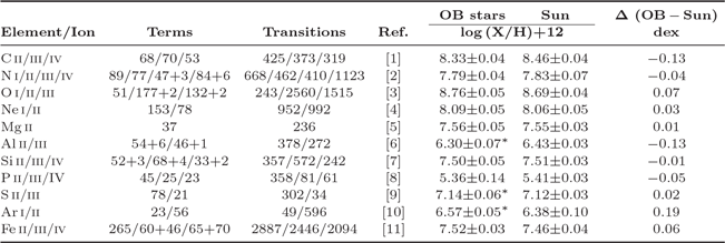
The number of superlevels is marked by a preceding ‘+’; photospheric abundances: Asplund et al. (Reference Asplund, Amarsi and Grevesse2021); $^*$ preliminary values. References: [1] Nieva & Przybilla (Reference Nieva and Przybilla2006); Nieva & Przybilla (Reference Nieva and Przybilla2008); [2] Przybilla & Butler (Reference Przybilla and Butler2001), Przybilla & Aschenbrenner (in prep.); [3] Przybilla et al. (2000), Aschenbrenner et al. (Reference Aschenbrenner, Przybilla and Butler2023); [4] Morel & Butler (Reference Morel and Butler2008); [5] Przybilla et al. (Reference Przybilla, Butler, Becker and Kudritzki2001a); [6] Przybilla (in prep.); [7] Przybilla & Butler (in prep.); [8] Aschenbrenner et al. (Reference Aschenbrenner, Butler and Przybilla2025); [9] Vrancken et al. (Reference Vrancken, Butler and Becker1996), updated; [10] Keiler et al. (in prep); [11] Becker (Reference Becker1998), Morel et al. (Reference Morel, Butler and Aerts2006).

A strength of the hybrid non-LTE approach is that highly detailed model atoms can be implemented, beyond hydrogen (Przybilla & Butler Reference Przybilla and Butler2004) and helium (Przybilla Reference Przybilla2005). An overview of the available model atoms for analysis of metals in OB stars in the hybrid approach is given in Table 1, where the element/ion combinations are listed, the number of energy terms and the number of radiative bound-bound transitions considered in the calculations. The model atoms typically also account for ab-initio data for photoionisation processes, and for a large number of electron-impact excitation data for a realistic description of also the local processes. Almost the entire optical spectra of OB stars can be reliably reproduced with these models.

Table 1.

Non-LTE model atoms and cosmic standard abundance data.

Table 1 Long description

A table comparing the abundance of various elements and ions in OB stars and the Sun. The table has 11 rows and 5 columns. The columns are labeled Element/Ion, Terms, Transitions, Ref., OB stars log (X/H)+12, Sun log (X/H)+12, and Δ (OB-Sun) dex. Each row lists an element or ion, the number of terms and transitions considered, a reference, and the logarithmic abundance values for OB stars and the Sun, along with the difference between them. For example, the first row lists C ii/iii/iv with 68/70/53 terms, 425/373/319 transitions, and a reference to [1]. The logarithmic abundance for OB stars is 8.33±0.04, for the Sun it is 8.46±0.04, and the difference is -0.13 dex.

Three codes are employed for spectral analyses, <sc>Spas</sc> (Hirsch Reference Hirsch2009), a more advanced semi-automated $\chi^2$-minimisation routine as described by Irrgang et al. (Reference Irrgang, Przybilla and Heber2014), and our most sophisticated code implemented so far, <sc>Saturn</sc> (Aschenbrenner & Przybilla, in prep.), which uses neural networks to emulate spectra of single and multi-star systems with arbitrary atmospheric parameters and chemical composition, and which offers a Markov-Chain Monte Carlo algorithm to derive stellar parameters and chemical abundances, and to constrain uncertainties. In all cases, synthetic spectra are used to fit multiple Stark-broadened hydrogen lines and multiple ionisation equilibria to derive the effective temperature $T_\mathrm{eff}$ and surface gravity $\log g$. Verification of $T_\mathrm{eff}$ can be achieved by fitting the spectral energy distribution (SED, which also provides information on interstellar reddening) and of gravity by a comparison of spectroscopic distances and those derived from parallaxes measured by the Gaia mission. The microturbulent velocity $\xi$ is constrained by requiring elemental abundances to be independent of strength of the spectral lines. Abundances are determined by line-profile fits to spectral lines, which requires the (projected) rotational velocity $v \sin i$ and (radial-tangential) macroturbulent velocity $\zeta$ to be constrained at the same time. Subsequently, fundamental stellar parameters, (evolutionary) mass M, radius R and luminosity L can also be determined, requiring stellar evolution models to be considered; see, e.g. Nieva & Przybilla (Reference Nieva and Przybilla2014). Alternatively, with the extinction constrained from the SED fit and the Gaia distance, one can derive the luminosity, and from this the radius (knowing $T_\mathrm{eff}$), and finally, using $\log g$, the (spectroscopic) mass.

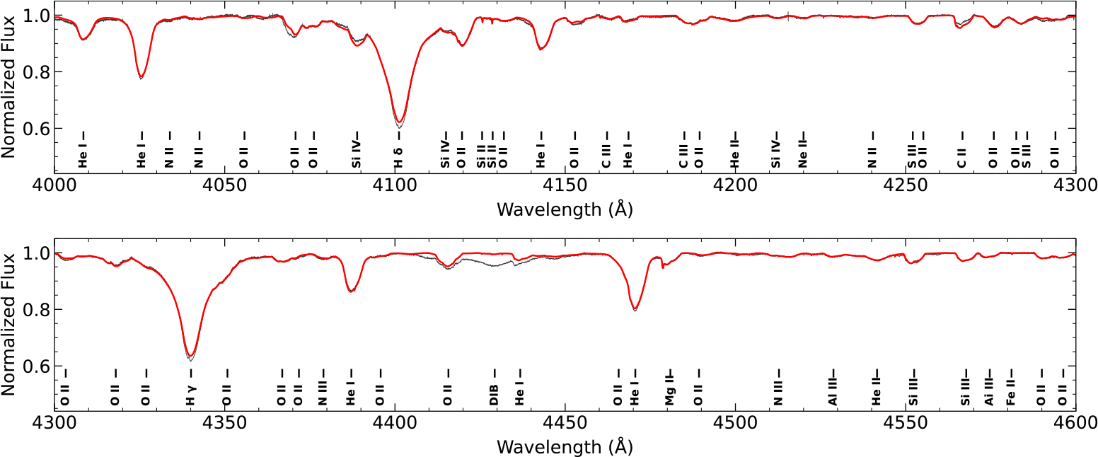
An example of the fit quality of a hybrid non-LTE model to an observed spectrum of a multiple star is shown in Fig. 1, the quadruple star system HD 37061, which excites the spherical H <sc>ii</sc> region Messier 43 close to the Orion nebula. The analysis (Aschenbrenner & Przybilla Reference Aschenbrenner and Przybilla2024) recovers abundances close to the cosmic standard abundances (see below). More examples, in particular of benchmark eclipsing binary systems, are discussed by Aschenbrenner & Przybilla (in prep.). The reliable reproduction of the observations is due to detailed model atoms and allows $T_\mathrm{eff}$, $\log g$ and elemental abundances to be determined with uncertainties of typically 1-2% and 0.05-0.10 dex (1$\sigma$ standard deviations) for the latter two, and absolute systematic uncertainties in abundances of $\sim$0.1 dex (e.g. Przybilla et al. 2000; Przybilla et al. Reference Przybilla, Butler, Becker and Kudritzki2001a; Przybilla et al. Reference Przybilla, Butler and Kudritzki2001b).

Figure 1.

Example of a model fit (red line) to an observed optical high-resolution spectrum (black) of a multiple star, the quadruple system HD 37061, exciting star of M 43 in Orion. Only the diffuse interstellar band at 4428 ${A}$ is unaccounted for by the model. Adopted from Aschenbrenner & Przybilla (Reference Aschenbrenner and Przybilla2024).

5. Observational constraints on massive star evolution from hybrid non-LTE analyses

Most of the stellar evolution tracks for Galactic massive stars employ a solar abundance mix of metallicity Z = 0.014 (Asplund et al. Reference Asplund, Grevesse, Sauval and Scott2009) as initial chemical composition input. This is because the most comprehensive information on chemical composition is available for the Sun (see Table 1 for photospheric abundances, the bulk abundances are about 0.04 dex higher), and it appears to reflect the elemental abundances in the solar neighbourhood rather well. On the other hand, it is not clear why a 4.6 Gyr old star should be chemically representative for the young massive star population – ever ongoing nucleosynthesis in the Milky Way should have increased the metallicity at the present Sun’s galactocentric radius over that time, depending on element, like 0.04 dex for oxygen to 0.14 dex for iron (Chiappini et al. Reference Chiappini, Romano and Matteucci2003).

Using hybrid non-LTE analyses, Przybilla et al. (Reference Przybilla, Nieva and Butler2008), Nieva & Simón-Díaz (Reference Nieva and Simón-Díaz2011) and in particular Nieva & Przybilla (Reference Nieva and Przybilla2012) studied a sample of slowly-rotating early B-type stars within a distance of $\sim$500 pc of the Sun and found chemical homogeneity. Data of the resulting cosmic abundance standard (CAS, plus results from later work on these and other OB stars) are summarised in Table 1. The comparison with solar photospheric abundances shows agreement for many elements but disagreement for some, in particular for carbon, aluminium, and argon. This is not in contradiction to Galactic chemical evolution. The data can be interpreted such that the Sun migrated radially in the Galactic disc from its birthplace about 2-3 kpc closer to the Galactic Centre to its current position (Wielen et al. Reference Wielen, Fuchs and Dettbarn1996; Nieva & Przybilla Reference Nieva and Przybilla2012).

Among the most recent applications of hybrid non-LTE models is the determination of the cosmic present-day abundance of phosphorus (Aschenbrenner et al. Reference Aschenbrenner, Butler and Przybilla2025). Its knowledge is important for reliable use of the typically unsaturated P <sc>v</sc> resonance lines as mass-loss indicators for hotter stars. The thus derived mass-loss rates are lower than those obtained from other indicators by about an order of magnitude, which was interpreted such that the radiatively-driven massive star winds are clumped (Fullerton et al. Reference Fullerton, Massa and Prinja2006). The revised mass-loss rates, in turn, have a great impact on stellar evolution models.

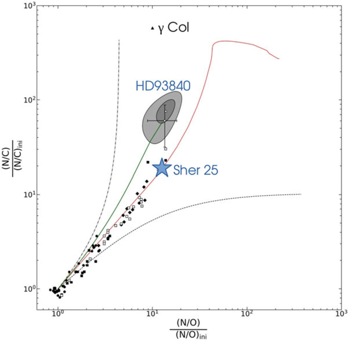
The small uncertainties in stellar parameters achievable via thorough hybrid non-LTE analyses enable a very accurate and precise positioning of the stars in the HRD, up to masses of $\sim$30 $M_\odot$ (because of the limitations of the hydrostatic model atmospheres); this applies also to the progeny of OB-type stars like BA-type supergiants (e.g. Przybilla et al. Reference Przybilla, Butler, Becker, Kudritzki and K. A.2006; Firnstein & Przybilla Reference Firnstein and Przybilla2012). Of particular interest are the thus obtainable observational constraints on rotational mixing in the course of stellar evolution, in the form of the abundances of carbon, nitrogen, and oxygen, indicators of the mixing of CNO-cycled matter from the core to the stellar surface. The analysed stars closely follow the path predicted by stellar evolution models in the N/C versus N/O diagram (Przybilla et al. Reference Przybilla, Firnstein and Nieva2010), see Fig. 2, implying also a high quality of the derived stellar parameters (Maeder et al. Reference Maeder, Przybilla and Nieva2014). The supergiants show overall a higher degree of mixing. Three recently analysed objects are highlighted in Fig. 2: the SN1987A progenitor-like Sher 25 with its hourglass-shaped surrounding nebula is one of the objects that shows the highest degree of mixing with nuclear-processed material, probably the result of a merger (for a further discussion see Weß mayer et al. 2023). HD93840, an extremely nitrogen-enhanced supergiant runaway star at intermediate galactic latitude with a previous binary mass-exchange history that also has a highly-processed bulk composition, indicating a very advanced stage in its evolution (Weß mayer et al. 2024); and $\gamma$ Col, which is a stripped and pulsating $\sim$4 to 5 $M_\odot$ core of an initially $\sim$12 ${M_\odot}$ star that just finished central hydrogen fusion (Irrgang et al. Reference Irrgang, Przybilla and Meynet2022). It mimics an ordinary early B-type subgiant spectrum, with the exception of near-equilibrium abundances of carbon and nitrogen from CN-cycle burning. The star is undergoing structural re-adjustment after the stripping event. Coming analyses of larger star samples with the hybrid non-LTE approach will provide detailed observational constraints on stellar evolution models, as they will also yield other fascinating outliers.

Figure 2.

N/C ratio vs. N/O ratios for a sample of OB stars (dots, filled boxes) and their progeny, BA-type supergiants (diamonds, open boxes), normalised to initial values. Three of the stars highlighted in the present work are marked. For comparison, the development of the surface CNO abundances is shown for two Geneva evolution tracks. The dashed and dash-dotted lines depict the analytical boundaries for the ON- and CN-cycle, respectively. Based on data described in detail by Weß mayer et al. (2024).

6. Pending issues

The imminent next challenges are indeed analyses of large spectroscopic datasets of thousands of massive stars, as will be provided by the William herschel telescope Enhanced Area Velocity Explorer (WEAVE, Jin et al. Reference Jin, Trager and Dalton2024) or the 4-metre Multi-Object Spectroscopic Telescope (4MOST, de Jong et al. Reference de Jong2019). Currently, several (semi)automated approaches exist for the analysis, such as, for example, genetic algorithms (Mokiem et al. Reference Mokiem, de Koter and Puls2005), grid-based $\chi^2$ minimisation algorithms (e.g. Araya et al. Reference Araya, Curé and Machuca2025), or codes such as <sc>Maui</sc> (Urbaneja Reference Urbaneja2026) that use a Markov chain Monte Carlo algorithm to constrain parameter sets and their uncertainties (for a first application see de Burgos et al. Reference de Burgos, Simón-Díaz, Urbaneja and Puls2024, on over 500 targets). First applications on hot stars were undertaken in the framework of the Gaia-ESO survey, on hundreds to thousands of stars (Blomme et al. Reference Blomme, Daflon and Gebran2022; Morel et al. Reference Morel, Blazère and Semaan2022). On a much larger scale, for about 330 000 OBA-type stars, the <sc>HotPayne</sc> code was employed for LTE modelling of the hot star content of the LAMOST survey (Xiang et al. Reference Xiang, Rix and Ting2022); a necessary extension is the consideration of non-LTE effects. Furthermore, an automated identification of binary and multiple stars with composite spectra also needs to be achieved in order to analyse these objects properly and in an automated fashion. In addition, outliers also need to be reliably identified automatically.

Further work is also required on tight empirical constraints on mass loss rates at all evolutionary stages of massive stars (including the RSG stage, where mass loss is supposed to be most efficient); this will have a noticeable effect on the reliability of stellar evolution models. Finally, – and this still requires a tremendous effort despite observational surveys such as BOB (Morel et al. Reference Morel, Castro and Fossati2015), BINAMICS (Alecian et al. Reference Alecian, Neiner and Wade2015) or MIMES (Wade et al. Reference Wade, Neiner and Alecian2016) that were targeted to spectropolarimetrically detect surface magnetic fields in massive stars –, additional input is required to derive observational constraints that will allow the generation and the impact of magnetic fields on massive star evolution to be quantified.