1 Introduction
1.1 A three-stage development
In recent years, we have witnessed increased interaction between agent-based computational economics (ACE) and econometricsFootnote 1. In this paper, we review the relationship between the two. While the link can be bi-directional, as we shall see in this survey, most of the work developed so far follows the direction from econometrics to ACE and has gradually consolidated ACE by shaping its econometric foundation. However, what is perhaps equally important and interesting is the reverse direction, that is, the potential influence of ACE on econometrics. One issue that has long concerned econometricians is the problem of aggregation over individuals, in particular when these individuals are heterogeneous and their composition is dynamically changing (Stoker, Reference Stoker1993; Gallegati et al., Reference Gallegati, Palestrini, Delli Gatti and Scalas2006). ACE, as a micro–macro model, serves as an ideal approach to studying this problem.
This survey article is, therefore, divided into three parts, which correspond to a three-stage development of the literature. The first two stages, namely, the econometric influence on ACE, examine the use of econometrics in ACE modeling. The first stage, entitled ‘presenting ACE with econometrics’, uses econometrics to analyze the data generated from the ACE models, and see whether they are able to display a number of frequently observed empirical features, that is, to replicate or grow ‘stylized facts’. At this stage, efforts are made to fine-tune the ACE model by matching the statistical properties of the real data with those of the artificial data to a qualitative precision. For example, if the real data exhibit the feature of volatility clustering, can a specific ACE model with a proper design generate data sharing the same feature? As we frequently experienced, there may be many designs, which are capable of featuring the same stylized fact; however, attempts to distinguish them were only made at the later (second) stage.
The concept of ‘optimizing’ ACE models with real data characterizes the development of the next stage, which is entitled ‘building ACE with econometrics’. In this stage, econometrics is used directly or indirectly, top-down or bottom-up, to estimate or calibrate ACE models. An attempt is made to construct ACE models that can replicate the stylized facts to a degree of quantitative precision, and, even more ambitiously, use ACE models to forecast the future.
The last part of the paper examines the above link in the reverse direction, that is, by looking at the influence of ACE on econometrics. In this third stage, entitled ‘emerging econometrics with ACE’, econometrics is still applied to the artificial data generated by ACE; however, instead of replicating the macroscopic structure, we examine whether the macroscopic structure described by the econometric results from the artificial data can be, in a sense, consistent with the micro-structure. This brings us to the elusive quest for a representative agent and the associated economic conditions for consistency in aggregation, an issue well discussed in both economic theory and econometrics (Kirman, Reference Kirman1992; Hartley, Reference Hartley1997; Casella et al., Reference Casella, Thoron and Trannoy2007).
However, the three-stage development sketched above is not generally shared by all economic research areas. The one, and probably the only one, which can demonstrate the three-stage development is finance or financial economics. This is because, over the last decade, the research area referred to as agent-based models of financial markets has grown very rapidly, and, in the meantime, financial econometrics has also experienced much prosperity. The two together happen to provide an excellent opportunity for us to examine the collaboration between ACE and econometrics. In this survey, we, therefore, review the three-stage development exclusively within this background. To make this focus sharp, we shall use the abbreviation ACF (agent-based computational finance), instead of ACE, when this specificity is clear.
1.2 Organization of the survey
Our survey mainly focuses on the concepts and the associated key questions appearing in each stage. For the first stage of the development, the question to address, given a set of stylized facts, concerns the elements that are needed to make an ACF model able to replicate those stylized features. By and large, we inquire how much of the causes of the stylized facts we can attribute to the heterogeneity and bounded rationality (learning) of agents, the two pillars of ACEFootnote 2. This naturally leads us to a taxonomy of ACF models based on the design of agents, also known as agent engineering Footnote 3.
In this paper, we consider two different designs of financial agents. The first design is referred to as the N-type design (Section 2.1), whereas the second design is referred to as the autonomous-agent (AA) design (Section 2.2). The most familiar example of the former is the fundamentalist-chartist model, and the most often cited example of the latter is the SFI (Santa Fe Institute) artificial stock market. The latter is more complex than the former in many ways, including the decision rules, the adaptive behavior, and the degree of heterogeneity among agents.
The two designs can be considered as two opposite positions in a spectrum as shown in Figure 1, which arranges the ACF models from simple to complex. This incremental process in design makes it easier for us to address the need for complex models. Specifically, Section 3 will address this issue: given the set of stylized facts that can be explained by the simple agent-based models, what is the additional explanatory power that can be gained by making more complex models? Can complex models grow or replicate more stylized facts? Section 3.1 provides a quick summary of those stylized facts based on the literature. Section 3.2 then analyzes how these stylized facts are successfully explained or replicated by various classes of ACF models.
A spectrum of agent-based computational finance models: heterogeneity

The same style of analysis is carried over in addressing the second stage of the development. At this stage, we ask what makes an ACE model econometrically tractable. Alternatively put, what are the necessary restrictions or assumptions that need to be imposed before an ACE model can be estimated? However, we will soon realize that the answer cannot be independent of the estimation method involved. This leads us to distinguish three main estimation methods, namely, maximum likelihood (MLE), least squares (LS), and the method of moments, as well as variations of the three. Generally speaking, the complexity of the objective function associated with the number of the parameters to be estimated will determine which of the estimation methods will be used. As a result, ACE models can also be categorized by the appropriate estimation method, which makes them econometrically tractable.
The questions addressed in the third stage are very different from those asked in the first two. The issue is not the empirical relevance or empirical validation of the built ACE models, but concerns using the ACE models as a tool to address the aggregation problem or the analogy principle, which has been extensively discussed in the literature (Blinder, Reference Blinder1983; Barker & Pesaran, Reference Barker and Pesaran1990; Forni & Lippi, Reference Forni and Lippi1997; Gallegati et al., Reference Gallegati, Palestrini, Delli Gatti and Scalas2006). In light of the Debreu-Mantel-Sonnenschein theorem, there are no grounds to expect macro behavior to be in any way similar or analogous to the behavior of individual agents. ACE models can help us to see how dissimilar the macro and micro behavior can be.
With the above description, the rest of the chapter is organized as follows. A taxonomy of ACE models is given in Section 2. The three-stage development of the literature is described in Section 3, Section 4, and Section 5. Concluding remarks are given in Section 6.
2 Taxonomy of agent-based computational economics models
In the middle and late 1990s, we began to see some of the attempts to use agent-based financial models to explain some empirical regularities observed from financial data. (Lux, Reference Lux1995, Reference Lux1997, Reference Lux1998; LeBaron et al., Reference LeBaron, Arthur and Palmer1999; Arifovic & Gencay, Reference Arifovic and Gencay2000). These attempts involve the use of very different agent-based models. To see how different they are, it is useful to categorize the ACF models by their density (simplicity or complexity) in terms of the three essential elements, namely, heterogeneity, learning, and interactions Footnote 4.
In terms of heterogeneity, we can distinguish simple heterogeneity from complex heterogeneity (LeBaron, Reference LeBaron2000). The former can be exemplified by the famous models of fundamentalists and chartistsFootnote 5, where there are only two different types of agents. The latter can be exemplified by the SFI artificial stock markets, where they are potentially infinite types of agents (Arthur et al., Reference Arthur, Holland, LeBaron, Palmer and Tayler1997). Regarding learning, there is also a spectrum from simple learning (algorithms) to complex learning (algorithms). Examples of the former are pure imitation and reinforcement learning, whereas examples of the latter are artificial neural networks (ANN), genetic algorithms (GAs), and genetic programming (GP)Footnote 6. Likewise, as for interactions, we can start from simple interactions, which either involve no network topologies or only simple networks, and progress to sophisticated interactions, which require complex network topologies.
With these three essential elements as the background, we shall start with the simplest possible class of ACF models, which is simple in each of the three elements, that is, simple heterogeneity, simple learning, and simple interaction. We then ask what are the stylized facts that can be accounted for by this simplest class of ACF models, and what are the stylized facts that are beyond their reachability. Using an incremental approach, we then ask how far we can move by gradually building more complex models, by being more complex in heterogeneity, learning, or interaction. From this gradual process, we can appreciate the contribution of each of the three elements to the emergence of the stylized facts. This way of organizing and presenting ACF models is similar to the inquiry into the necessary and sufficient conditions of the stylized facts.
2.1 N-type designs
In reality, financial agents can differ in many dimensions, ranging from expectations formation (beliefs), trading strategies, information exposure, risk attitudes, wealth (investment scale), and the need for liquidity, etc. Given this high-dimensional heterogeneity, the essential question for financial agent engineering is to decide how much heterogeneity is to be reflected in the artificial markets. How much more coarsely or finely do we want to differentiate these financial agents?
Before we examine the design of artificial financial agents, it is useful to recall what we have done for other artifacts. To name a few, the design of artificial ants (ant algorithms) was motivated by observing the behavior of real ants in a laboratory; the design of artificial bacteria (bacterial algorithms) was inspired by the microbial evolution phenomenon; the design of the artificial brain (neural networks, self-organizing maps) was motivated by the study of the real human brain; and the design of the evolutionary process (evolutionary algorithms) was inspired by real biological evolution. Generally speaking, the design of an artifact is, by and large, motivated and guided by the behavior of its counterpart in nature.
The design of artificial financial agents is no exception. It is highly motivated by observing how real financial agents behave. Empirical evidence accumulated since the late 1980s and early 1990s has shed new light on the forecasting behavior of financial agents. This empirical evidence was obtained through different kinds of surveys, such as questionnaires and telephone interviews, with financial specialists, bankers, currency traders, and dealers, etc. (Allen & Taylor, Reference Allen and Taylor1990; Frankel & Froot, Reference Frankel and Froot1990). The general findings from these abundantly established empirical data are twofold. First, the data indicate that, by and large, there are two kinds of expectations existing in the market. The expectation characterized as a stabilizing force of the market is associated with a type of financial agent, called the fundamentalist. The expectation characterized as a destabilizing force is associated with another type of financial agent, called the chartist, technical analyst or trend extrapolator. Second, the proportion (micro-structure) of fundamentalists and chartists, also called the market fraction, is changing over time, which indicates the adaptive aspects of financial agents. These empirical findings provide the initial direction for the early development of financial agent engineering. First, they suggest what rules to look at; second, they point out the significance of learning and adaptation.
Fundamentalists and chartists are concerned with two very different beliefs regarding stock price dynamics. In a simple setting, they differ in terms of the mean-reverting speed of the stock price when it is mispriced (undervalued or overvalued). Fundamentalists tend to believe that the mispriced situation will soon be corrected, whereas chartists tend to believe that in the short run it will continue.
2.1.1 Two-type and three-type designs
Among all classes of ACF models, obviously the two-type design is the simplest kind of heterogeneity which one can have. There is a precise behavioral rule for each type of agent. In each period of time, each agent has to choose one of these two types, and this choice will be reviewed and revised constantly. Hence, in the next period, agents may switch between the two types. Learning and interaction are both encapsulated in the switching mechanism, that is, the binary-choice model, the simplest discrete-choice model.
To make this design more precise, we denote the forecasting rule of a type-h agent in the general sense as follows:

where Eh,t refers to the expectations of the type-h agent at time t. Equation (1) indicates the one-step ahead forecast. At the beginning, we start with a very general forecasting function fh,t, which uses all the historical data on price up to the present. In addition, considering that agents are adaptive, we allow the function to change over time and hence denote it by the subscript t.
For the fundamentalists (h = f) and chartists (h = c), their forecasting rules, in a very simple setting, can be written as


Among all classes of ACF models, the simplest class that can serve as a starting point is that of the two-type models. These models have two types of agents, and they differ in their beliefs and the associated trading strategies. While one of these two types of agents is always called fundamentalists, the other may have different names, such as chartists, technical traders, trend-followers, or noisy traders.
The idea behind these two behavioral rules is that the fundamentalist has a mean-reverting belief, and his belief is characterized by a reverting coefficient (αf), whereas the chartist has the trend-continuing belief, and his belief is characterized by an extrapolating coefficient (αc). The magnitude of the reverting coefficient (αf) measures the speed with which the fundamentalists expect the price to return to the fundamental price ( ), whereas the magnitude of the extrapolating coefficient (αc) expresses the degree to which chartists extrapolate the past change into the future.
Three-type designs. There is little doubt that the behavior of financial agents can be more complex than the two-type design. One obvious way to scale-up this design is to add more types of agents to the model so as to take into account a finer degree of heterogeneity of financial agents. This type of expansion is called the N-type design. For example, in a three-type design, one can further distinguish two kinds of chartists, namely, momentum traders and contrarian traders, or simply, contrarians. Like momentum traders, contrarians extrapolate past movements of the price into the future, but they follow the opposite of the trend. More precisely, their forecasting rule is as follows:

Contrarians consider that the price trend will finish soon, and then start to reverse. However, unlike fundamentalists, contrarians do not base their forecasts on the fundamental price, which they either do not know, or do not care about.
The recent availability of more proprietary data has enhanced the transparency of the trading behavior of financial agents, including both individual and institutional investors. Empirical studies using such data have shown that individuals and institutions differ systematically in their reaction to past price performance and the degree to which they follow momentum and contrarian strategies. On average, individual investors are contrarian investors: they tend to buy stocks that have recently underperformed the market and sell stocks that have performed well in recent weeks (Barber & Odean, Reference Barber and Odean2000). With this empirical basis, financial agent engineering has already added the contrarians to the fundamentalist–chartist model, and popularized this three-type designFootnote 7.
Generalization of two- and three-type designs. Financial agent engineering can also be advanced by enriching the behavioral rules associated with each type of financial agent. This alteration may make financial agents more interdisciplinary. Considerations from different fields, including the neural sciences, cognitive psychology, and statistics, can be incorporated into designs. For example, in behavioral finance, there is a psychological bias known as the ‘law of small numbers’, which basically says that people underweight long-term averages, and tend to attach too much weight to recent experiences (the recency effect). When equity returns have been high for many years, financial agents with this bias may believe that high equity returns are ‘normal’. By design, we can take such bias into account. One way to do so is to add a memory parameter to the behavioral rules of our financial agents. This more general rule for contrarians is specified as follows:


The momentum traders and contrarians now compute a moving average of the past changes in the stock price and extrapolate these changes into the future of the stock price. However, we assume that there is an exponential decay in the weights given to the past changes in the stock price. The parameters βc and βco can be interpreted as reflecting the memory of momentum traders and contrarians. If βc = βco = 0, momentum traders and contrarians remember only the last period's price change and they extrapolate this into the future. When βc and βco increase, the weight given to the price changes farther in the past increases. In other words, the chartists’ memory becomes longer.
The psychological bias mentioned earlier, therefore, corresponds to a small value of this memory parameter, and this ‘hypothesis’ can actually be tested (Amilon, Reference Amilon2008)Footnote 8.
Adaptive behavior. In the original fundamentalist–chartist model, learning does not exist. Agents who initially happen to be fundamentalists will continue to be fundamentalists and will never change this role, and likewise for chartists. As a result, the proportion (market fraction) of fundamentalists and chartists remains fixed. Nonetheless, this simplification underestimates the uncertainty faced by each trader. In general, traders, whether they are fundamentalists or chartists, can never be certain about the duration of the biased trend, since the trend can finish in weeks, months, or years. This uncertainty causes the alerted traders to review and revise their beliefs constantly. In other words, traders are adaptive.
Therefore, a further development of financial agent engineering is to consider an evolving micro-structure of market participants. In this extension, the idea of adaptive agents or learning agents is introduced into the model. Hence, an agent who was a fundamentalist (chartist) may now switch to being a chartist (fundamentalist) if he considers this switching to be more promising. Since, in the two-type model, agents can only choose to be either a fundamentalist or a chartist, modeling their learning behavior becomes quite simple, and is typically done using a binary-choice model, specifically, the logit model or the Gibbs–Boltzmann distribution (Luce, Reference Luce1959; Blume, Reference Blume1993).
The logit model, also known as the Luce model, is the main model used in the psychological theory of choice. Consider two alternatives, f (fundamentalist) and c (chartist). Each will produce some gains to the agent. However, since the gain is random, the choice made by the agent is random as well. The logit model assumes that the probability of the agent choosing f is the probability that the profits or utilities gained from choosing f are greater than those gained from choosing c. Under a certain assumption for the random component of the utility, one can derive the following binary logit model:Footnote 9

where Vf,t and Vc,t are the deterministic components of the gains from the alternatives f and c at time t. The parameter λ is a parameter carried over from the assumed random component. The logit model says that the probability of choosing the alternative f depends on its absolute deterministic advantages, as we can see from the following reformulation:

When applied to agent-based financial models, these deterministic components are usually related to the temporal realized profits associated with different forecasting rules. So, in the two-type model, Vf,t is the temporal realized profits from being a fundamentalist, and Vc,t is the temporal realized profits from being a chartist. In addition, there is a new interpretation for the parameter λ, namely, the intensity of choice, because it basically measures the extent to which agents are sensitive to the additional profits gained from choosing f instead of c.
Market-maker equation. The distribution function above then determines the market fraction of each type of agent in the market. For example, if Prob(X = f) = 0.8, it means that 80% of the market participants are fundamentalists and the remaining 20% are chartists. The asset price will be determined by this market fraction via the market-maker equation:

where

Equation (9) is the market-maker equation, which assumes that the price is adjusted by the market maker, whose decision is in turn determined by the excess demand normalized by the number of market participants, Dt. Dt, in Equation (10), is a weighted average of the individual demand of each type of trader, weighted by the market fractions (7).
An alternative to determine the market price is through the familiar Walrasian equilibrium, which is also frequently used in ACF models.
Risk preference and portfolio. Demand for the assets of each type of trader is derived in a standard expected-utility maximization manner, and depends on the risk preference of the type-h agent. Risk preference is important because it is the main determinant of agents’ portfolios, that is, how agents’ wealth is distributed among different assets. The classical Markowitz mean–variance portfolio selection model offered the first systematic treatment of asset allocation. Harry Markowitz, who received the 1990 Nobel Prize in Economics for this contribution, assumes that investors are concerned only with the mean and variance of returns. This mean–variance preference has been extensively applied to modeling agents’ risk preferences since the variance of returns is normally accepted as a measure of risk.
In addition to the mean–variance preference, there are two other classes of risk preferences that are widely accepted in the standard theory of finance. These two correspond to two different attitudes toward risk aversion. One is called constant absolute risk aversion (CARA), and the other is called constant relative risk aversion (CRRA). When an agent's preference exhibits CARA, his demand for the risky asset (or stock) is independent of his changes in wealth. When an agent's preference exhibits CRRA, his demand for risky assets will increase with wealth in a linear way. Using a Taylor expansion, one can connect the mean–variance preference to CARA preferences and CRRA preferences. In fact, when the returns on the risky assets follow a normal distribution, the demand for risky assets under the mean–variance preference is the same as that under the CARA preference, and is determined by the subjective-risk-adjusted expected return.

where Δpt + 1 = pt + 1 − pt and ah,t is a risk aversion coefficient. The Eh,t(pt + 1) in the numerator of Equation (11) is given by Equations (2)–(4), and the σh,t in the denominator represents the perceived risk by the type-h agents. Further details of the formation of this subjective perceived risk can be found in the agent-based finance literature (De Grauwe & Grimaldi, Reference De Grauwe and Grimaldi2006; Hommes, Reference Hommes2006).
2.1.2 Many-type designs
Adaptive belief systems (ABS). Brock and Hommes (Reference Brock and Hommes1997, Reference Brock and Hommes1998) initiate an N-type design called the ABS. This system can be considered to be an extension of the two-type or three-type design, which we observed earlier. In this case, there are more than two or three kinds of beliefs in the market, and the number is denoted by N. Like the two- or three-type designs, each of these beliefs is known in advance and is fixed. Brock and Hommes (Reference Brock and Hommes1998) further assume that they are all linear forecasting rules, as follows:

In this simplification, each belief is characterized by a set of coefficients (αh ,0, αh ,1, …, αh ,L + 1), denoted by  . The adaptation part or the switching mechanism can be easily extended from the original logit model (Equation (7)) into the multinomial logit model:

The rest of the ABS is essentially the same as the few-type designs.
Large type limit (LTL) and continuous belief systems (CBS). One further extension of the N-type design is to consider not just a finite N but an infinite N, that is, N→∞. In this line, Brock et al. (Reference Brock, Hommes and Wagener2005) introduce the notion of a LTL, whereas Diks and van der Weide (Reference Diks and van der Weide2005) propose a CBS. They both rely on the idea of a distribution of beliefs. The distribution of beliefs is a distribution over a belief space, from which the observed beliefs are sampled. When the belief space is a space of real numbers, one will then have an infinite-type design. The earlier finite N-type design can be regarded as a sample with size N from this distribution. Once it is generated, the sample is fixed, and then later on the adaptation or switching mechanism is just operated within this fixed sample. However, the infinite N-type design works directly on the population of beliefs, instead of a sample of beliefs. Since the distribution of beliefs can be captured by a few parameters, one can effectively use a small number of parameters to represent a large number of different types of traders. The discrete-choice problem is now expanded into a continuous-choice problem, but still with the Gibbs–Boltzmann distribution.

‘Type’ in few-type and many-type designs. While the large-type design can be considered to be a natural mathematical extension of the few-type design, one should notice that it does have a dramatically different notion of type. The notion of type in the few-type designs is in fact a cluster, that is, a cluster of similar trading strategies or beliefs. Therefore, while there are a large number of traders in the world, their behavior is limited to just a few clusters or a few typesFootnote 10. The early literature on fundamentalists and chartists is developed in this fashion. In other words, they are two different types, not because they are different, but because they are fundamentally different. Two fundamentalists may still have different beliefs, but compared with those of chartists, their differences are negligible. The large-type designs no longer keep this notion of a cluster; instead, traders with even an arbitrarily small difference are considered to be different types by them.
2.1.3 Illustrations
In the literature, there are three major N-type ACF models; in chronological order, they are the Kirman model, the Lux model, and the Brock–Hommes model. The entire structure of Section 2.1.1 is written by largely following the Brock–Hommes ABS model. Section 2.1.2 also provides the extension of the ABS model. Therefore, only the Kirman and Lux models will be highlighted here.
Kirman's ANT model. Kirman's model was first proposed by (Kirman, Reference Kirman1991, Reference Kirman1993). It is a two-type model. The two types are fundamentalists and chartists. The model, however, differs from the previous description of the two-type model in its switching mechanism. The switching is not driven by the Gibbs–Boltzmann distribution (Equation (7)), but by a herding mechanism. Within this herding mechanism, the main determinant of the respective binary choice is not the financial success (the Vf,t and Vc,t appearing in Equation (7)) but the fraction of the majority. Therefore, the decision is more psychologically than economically driven.
The herding mechanism was inspired by an observation in entomology. ‘Ants, faced with two identical food sources, were observed to concentrate more on one of these, but after a period they would turn their attention to the other’ (Kirman (Reference Kirman1993), p. 137). Inspired by observing the behavior of ants, Kirman characterizes the switching potential of each individual by two parameters, namely, a probability of self-conversion and a probability of being converted. The self-conversion probability gives rise to the probability that an individual will switch to other types of agents without external influence, whereas the probability of being converted gives rise to the probability that the individual will be persuaded by the other individual with whom he is randomly matched. This switching process is discrete and can be studied in a general theoretical framework of a Polya urn process.
Lux's IAH (interactive agent hypothesis) model. The Lux model was initiated by Lux (Reference Lux1995, Reference Lux1997, Reference Lux1998). It is a hierarchical two-type model. It is hierarchical in the sense that there are fundamentalists and chartists, but the chartists are further divided into optimists and pessimists. Like the Kirman model, the Lux model also has the herding element. However, the original discrete-time discrete-choice behavior in the Kirman model is now replaced by a continuous-time discrete-choice model. This change has caused the Lux model to have a very different mathematical structure, which is a jump Markov process. In such continuous-time mathematics, the switching mechanism among the three groups of agents is captured by the transition rate function.
The transition rate specifies the change rate of the conditional probability of shifting to another state after an infinitesimal time interval that is conditional upon a specific current state. The state refers to each possible distribution (each set of fractions) over the types (clusters). For example, in a two-type model, the distribution at a point in time can be characterized by one parameter, that is, the fraction of type one, say, w 1(t), since subtracting it from unity gives the fraction of type two, that is, w 2(t) = 1 − w 1(t).
Lux considers two determinants in the transition rate function. One is the profit differential, that is, the difference in trading profits between the fundamentalists and chartists. The transition rate function is negative in the profit differentials between own profits and alternative profits. In this way, as expected, when fundamentalists earn a higher profit than chartists, it will become less likely for a fundamentalist to switch, but more likely for a chartist to switch. Hence, in this regard, it is very similar to the Gibbs–Boltzmann distribution used by Brock and Hommes’ ABS. The other determinant is herding. In this case, traders’ decisions to switch between different clusters are affected by the number of traders in each cluster. The majority cluster may find it easier to attract traders from the minority cluster, but this is less likely to happen the other way round. In the Lux model, herding is only applied to the switch between optimists and pessimists.
Minority games (MG). Since trend-chasers and contrarians in the financial market can be positioned as the majority and minority, a mixed minority and majority game, also known as an $-game, has been applied to agent-based financial markets (Challet & Zhang, Reference Challet and Zhang1997). There are some designs of agents that can be particularly suitable for the MG models. One example is the threshold model proposed by Ghoulmie et al. (Reference Ghoulmie, Cont and Nadal2005) and Cross et al. (Reference Cross, Grinfeld, Lamba and Seaman2007).
2.2 Autonomous-agent designs
In the N-type designs, all the types and rules of financial agents are given at the beginning of the design, and what financial agents can do is to choose among these different types or rules based on their past experiences. The N-type design has characterized a major class of agent-based financial markets. However, this way of doing things also severely restricts the degree of autonomy available to financial agents. First, they can only choose how to behave based on what has been offered; secondly, as a consequence, there will be no new rules available unless they are added exogenously by the designers. If we want our artificial financial agents to behave more like real financial agents, then we will certainly expect that they will learn and discover on their own. Therefore, as time goes by, new rules that have never been used before and have not been supplied by the designer may be discovered by these artificial agents inside the artificial world.
2.2.1 The sante fe institute artificial stock market
GAs. Designing artificial agents who are able to design on their own is an idea similar to John von Neumann's self-reproducing automata, that is, a machine that can reproduce itself. This theory had a deep impact on John Holland, the father of the GA. Under von Neumann's influence, Holland devoted himself to the study of a general-purpose computational device that could serve as the basis for a general theory of automata. In the 1970s, he introduced the GA, which was intended to replace those ad hoc learning modules in contemporary mainstream Artificial intelligence. Using GAs, Holland could make an adaptive agent that not only learned from experience but could also be spontaneous and creative. The latter property is crucial for the design of artificial financial agents. In 1991, Holland and John Miller, an economist, published a sketch of the artificial adaptive agent in the highly influential American Economic Review (Holland & Miller, Reference Holland and Miller1991). This blueprint was actually carried out in an artificial stock project in 1988 at the SFI (Palmer et al., Reference Palmer, Arthur, Holland, LeBaron and Tayler1994; Arthur et al., Reference Arthur, Holland, LeBaron, Palmer and Tayler1997).
Armed with GAs, the Santa Fe Artificial Stock Market (SFI-ASM) considers a novel design for financial agents. First, like many N-type designs, it mainly focuses on the forecasting behavior of financial agents. Their trading behavior, as depicted in Equation (11), will depend on their forecasts of the price in the next period. Second, however, unlike the N-type designs, these agents are not divided into a fixed number of different types. Instead, the forecasting behavior of each agent is ‘customized’ via a GA. We shall be more specific regarding its design because it provides us with a good opportunity to see how economists take advantage of the increasing computational power to endow artificial decision makers with a larger and larger degree of autonomy.
In the SFI-ASM, each financial agent h uses a linear forecasting rule as follows:

However, the coefficients αh,t and βh,t not only change over time (are time-dependent), but are also state-dependent. That is, the value of these two coefficients at time t will depend on the state of the economy (market) at time t. For example, the recent price dynamics can be an indicator, so, say, if the price has risen in the last three periods, the financial agent may consider lower values of both α and β than otherwise. The price dividend ratio can be another indicator. If the price dividend ratio is lower than 50%, then the financial agent may want to take a higher value of β than if it is not. This state-dependent idea is very similar to what is known as classification and regression trees or decision trees, a very dominant approach in machine learning.
Therefore, one simple way to think of the artificial agents in the SFI-ASM is that they each behave as machine-learning people who use regression trees to forecast the stock price. At each point in time, the agent has a set of indicators, which help him to decompose the state of the economy into m distinct classes  , and corresponding to each of the classes there is an associated linear forecasting model. Which model will be activated depends on the state of the market at time t, denoted by St. Altogether, the behavior of the financial agent can be summarized as follows:

A few remarks are added here. First, the forecasting rule summarized above is updated as time goes by, as we keep the subscript t there. So, agents, in this system, are learning over time with a regression tree, or they are using a time-variant regression tree, in which all the regression coefficients and classes may change accordingly with the agents’ learning. Second, agents are completely heterogeneous, as we also keep the subscript h above. Therefore, if there are N financial agents in the market at each point in time, we may observe N regression trees, each of which is owned and maintained by one individual agent. Third, however, the forecasting rules introduced in the SFI-ASM are not exactly regression trees. They are, in fact, classifier systems.
Classifier system. A classifier system is another of John Holland's inventions from the late 1970s (Holland, Reference Holland1975). It is similar to the Newell–Simon type of expert system, which is a population of if-then or condition-action rules (Newell & Simon, Reference Newell and Simon1972). Conventional expert systems are not able to learn by themselves. To introduce adaptation into the system, Holland applied the idea of market competition to a society of if-then rules. A formal algorithm, known as the bucket-brigade algorithm, credits rules generating good outcomes and debits rules generating bad outcomes. This accounting system is further used to resolve conflicts among rules. The shortcoming of the classifier system is that it cannot automatically generate or delete rules. Therefore, a GA is applied to evolve them and to discover new rules.
This AA design has been further adopted in many later studies. While most studies continuously carried out this task using GAsFootnote 11, a few studies also used other population-based learning models, such as evolutionary programming, GP, and particle swarm optimization.
2.2.2 Genetic programming and autonomous agents
The development from the few-type designs to the many-type designs and further to the AA designs can be considered to be part of a continuous effort to increase the collective search space of the forecasting function Eh,t, from finite to infinite space, and from parametric to semi-parametric functions. The contribution of GP to this development is to further extend the search space to an infinite space of non-parametric functions, whose size (e.g. the dimensionality, the cardinality, or the number of variables used) and shapes (e.g. linearity or nonlinearity, continuity or discontinuity) have to be determined, via search, simultaneously. This way of increasing the degree of autonomy may not contribute much to the price dynamics, but it can enrich other aggregate dynamics as well as the behavior at the individual level. As we shall see below, the endogenous determination of the size and shape of Eh,t provides us with great opportunities to see some aspects of market dynamics, which are not easily available in the N-type designs or other AA designs.
The first example is about the sophistication of agents in market dynamics. The definition and operation of GP (Koza, Reference Koza1993) rely on a specific language environment, known as LIST Programming (LISP). For each LISP program, there is a tree representation. The number of nodes (leaves) or the number of depths in the LISP trees provides one measure of complexity in the vein of the program length. This additional observation enables us to study not just the heterogeneity in Eh,t, but also the associated complexity of Eh,t. In other words, GP cannot only distinguish agents by their forecasts, as the N-type designs did, but can further delineate the differentiation based on the agents’ sophistication (complexity). Must the surviving agents be sophisticated or can the simple agents prosper as well?
One interesting hypothesis related to the question above is the monotone hypothesis: the degree of traders’ sophistication is an increasing function of time. In other words, traders will evolve to be more and more sophisticated as time goes on. However, this hypothesis is rejected in Chen and Yeh (Reference Chen and Yeh2001). They found that, based on the statistics on the node complexity or the depth complexity, traders can evolve toward a higher degree of sophistication; at some point in time, they can be simple as well.
The second example concerns the capability to distinguish the information from noise. As we mentioned earlier, the variables recruited in the agents’ forecasting function are also endogenously determined. This variable-selection function allows us to examine whether the smart pick of these variables is crucial for their survival. In particular, the hypothesis of the extinction of noisy traders says that traders who are unable to distinguish information from noise will become extinct. Chen et al. (Reference Chen, Liao and Chou2008) test this hypothesis. In an agent-based artificial market, they supplied traders with both the informative and noisy variables. The former includes prices, dividends, and trading volumes, whereas the latter are just series of pseudo-random numbers. Their simulation shows, as time goes on, that traders who are unable to distinguish information from noise do have a tendency to decline and even become extinct.
2.3 Heterogeneity in N-type designs and autonomous-agent designs
However, the AA design is not entirely the same as the N-type design built upon the discrete-choice or continuous-choice modelsFootnote 12. The main difference lies in learning. While both designs consider evolutionary selection as an essence of learning, their technical implementations are different, which also introduces some conceptual differences between the two.
The evolutionary selection mechanisms used in the discrete-choice or continuous-choice models simply assume that all agents are homogeneous in the sense that they are facing the same uncertainty when making their choices. It is the randomness of their choices (stochastic choices) that makes them behave differently. In other words, all agents are homogeneous ex ante, but heterogeneous ex post. However, this assumption or restriction may not generally apply to the SFI models.
Depending on the specific setting, the SFI models can allow agents to be truly heterogeneous in the sense that not only can they be heterogeneous ex post, but they can also be heterogeneous ex ante, that is, each agent's stochastic choice can come from his own idiosyncratic distribution. A typical example is the SFI model whose agents are modeled via multi-population GAs or multi-population GP (Yeh & Chen, Reference Yeh and Chen2001). In these examples, each agent learns from his own experiences rather than from a socially shared experience, as the one used in a multi-nominal logit model. This style of learning is known as individual learning in the literature, which is distinct from social learning (Vriend, Reference Vriend2000, Reference Vriend2002; Arifovic & Maschek, Reference Arifovic and Maschek2006).
Other variants of agent-based computational models go further to consider agents with varying degrees of learning capabilities. For example, Chan et al. Reference Chan, LeBaron, Lo and Poggio1999 consider three classes of forecasting agents in their artificial stock market, namely, empirical Bayesian traders, momentum traders, and nearest-neighbor traders. Yang (Reference Yang2002) also considers a mixture of a class of ANN agents and and a class of momentum agents. In each class, agents can be further distinguished by the specific parameters used to articulate their forecasting or trading behavior.
To sum up, the movement from the two-, many- to infinite-type models, and its further jump to the computational models can be characterized by a higher degree of heterogeneity and also a more complex learning behavior. The question is what benefit can we gain from this? Can we explain more stylized facts than the baseline models?
3 Presenting agent-based computational economics with econometrics
3.1 Stylized facts
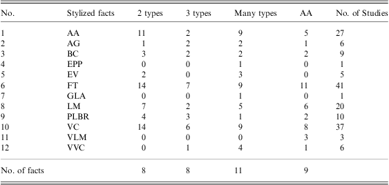
The first contact between ACE and econometrics was motivated by examining whether ACE models are able to provide explanations for some stylized features, which the existing economic theories have difficulties accounting for. The most notable examples can be found in the modern financial literature, with a list of stylized facts, which cannot be easily accounted for by the long-standing standard asset-pricing models built upon the device of representative agents. These stylized facts include statistical properties of various trading data, such as trading volume, and trading duration, but mostly concentrate on asset return. Table 1 provides a comprehensive coverage of these stylized facts.
Stylized facts

The stylized facts are separated into six blocks in the table. The first two refer to the stylized facts pertaining to return and trading volume, using low-frequency data. The next four refer to the stylized facts of return, trading duration, transaction size, and bid-ask spread, using high-frequency data.
There is a total of 30 stylized facts listed in this table, which are separated into six blocks. The first two blocks refer to the stylized facts of low-frequency financial time series, whereas the last four blocks refer to the stylized facts of high-frequency ones. The first two blocks give the stylized facts of returns and trading volume. The last four blocks refer to the stylized facts of returns, trading duration, transaction size, and bid-ask spreadFootnote 13.
3.2 Facts to be explained
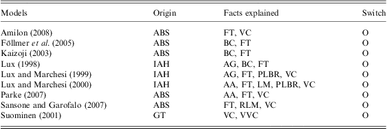
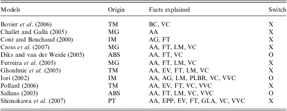
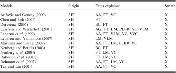
Can the above stylized facts be generated from a collection of interacting software agents? To see the bigger picture, a few tables are prepared to answer this question. We first categorize all ACF models based on the taxonomy given in Section 2. Some selected ACF models are separately listed in Tables 4–6 (see Appendix A), based on their designs being two-type, three-type or many-type, whereas another group of ACF models using the AA design is listed in Table 7 (also in Appendix A). The four tables together include 50 ACF models, among which there are 38 N-type models and 12 AA models; the ratio of the two is 3:1. The constituents of the N-type models are 18 (47%) two-type models, 9 (24%) three-type models, and 11 (29%) many-type models.
3.2.1 Demographic structure
These four tables are by no means exhaustive, but comprise just a sample of a large pile of existing studies. Nonetheless, we believe that they well represent some basic characteristics of the underlying large pile of literature. First, the largest class of ACF models is the few-type design. The sum of the two-type and three-type models account for about 50% of the entire sample. The few-type design models not only have support from empirical studies, but their simplicity also facilitates analytical work. This is probably the most important reason for seeing the dominance of this few-type design. Nonetheless, if a large degree of heterogeneity can be represented by a parametric distribution, then one can directly work with this distribution so as to extend the analytical work to the many-type designs. Using the continuous-choice model to replace the discrete-choice model is one case in point. This helps N-type design models gain an additional market share of 20–25%. The residual goes to the AA design models, which only take up one-fourth of the sample. This minority position may indicate that economists are not yet ready to accept the complex heterogeneous agents, which may easily defy analytical feasibility, but the more important question is: can more complex designs provide us with better explanatory power?
3.2.2 General performance
In Tables 4–7, the sides with each ACF model are shown to be the stylized facts that ‘can’ be replicated by the designated model. We have to be careful as to what we mean by ‘can’. First, we do not verify the model, and hence do not stand in a position to provide a second check as to whether the reported results are correct. In this regard, we assume that the verification of each model has been confirmed during the refereeing process. Second, we do, however, make a minimal effort to see whether proper statistics have been provided to support the claimed replication. A study that does not satisfy this criterion will not be taken seriously.
In addition, column 2 contains acronyms, which stand for the origin of the respective ACF models. Those origins have been briefly reviewed or mentioned in Section 2. In addition, the last column in each table serves to show whether the ACF model has a switching mechanism to allow agents to change their type. Switching or evolving fractions have been considered to be a fundamental cause of many stylized facts (Kirman, Reference Kirman1991, Reference Kirman1993; Lux & Marchesi, Reference Lux and Marchesi1999, Reference Lux and Marchesi2000; Hommes, Reference Hommes2002). Therefore, it is useful to have this information to examine whether the evolving fraction is a necessary condition for replicating stylized facts.
We shall start with the overview table (Table 2). A quick grasp begins with the last column of the table, which is a frequency count of the replications of the respective stylized facts shown in the first column. While there are 30 stylized facts shown in Table 1, only 12 (12 rows) appear in Table 2. The stylized facts that do not appear in this table are the facts that have not been replicated in any of the 50 papers in our survey. As a result, all stylized facts pertaining to the high-frequency data, or the so-called intraday data, are left unexplained by the ACF models, which include high-frequency returns (18–22; Table 1), trading duration (23–25), transaction size (26–27), and the bid-ask spread (28–30). In fact, even for those stylized facts appearing in the table, the counts associated with them are quite uneven.
Summary of stylized facts explained
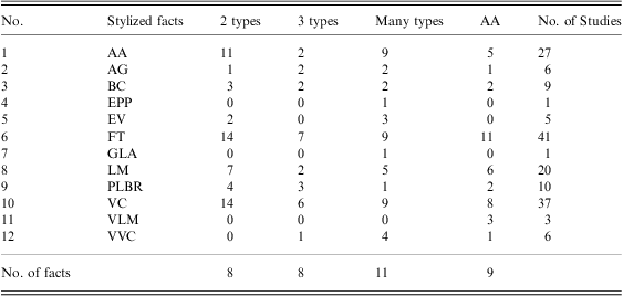
The last row ‘No. of facts’ is the total number of stylized facts that are replicated by the corresponding class of agent-based computational finance models. So, for example, the numbers 8, 8, 11, and 9, appearing in the last row, indicate that there are a total of eight stylized facts replicated by the two-type models, eight stylized facts replicated by the three-type models, and so on and so forth. It is not the total sum of the number appearing in the respective column.
First, there are four stylized facts, which clearly receive more intensive attention than the others. These four are fat tails (41 counts), volatility clustering (37), absence of autocorrelation (27), and long memory of returns (20). Fat tails and volatility clustering received the highest attention. This, in fact, is well anticipated, given the close connection between the two and the dominance of various GARCH (Generalized AutoRegressive Conditional Heteroskedasticity)-type models in financial econometricsFootnote 14. Long memory ranks fourth. This again is closely related to volatility clustering, since long memory reflects long-run dependencies between stock market returns, and volatility clustering describes the tendency of large changes in asset prices to follow large changes, and small changes to follow small changes.
Second, we also notice that all stylized facts explained exclusively pertain to asset prices; in particular, all these efforts are made to tackle the low-frequency financial time series. This sharp bias is also not difficult to understand. Although most ACF models have their own artificial clock, it is not clear what the interval [t,t + 1] can best mean in real time. Does it refer to a tick, a minute, an hour, a day or a week? There is no easy way in which we can tell the difference from the corresponding models. The difference can only be made via the empirical part of the models, which requires a consideration of which dataset is involved. Since the high-frequency dataset is rarely used as the empirical correspondence of these ACF models, it remains a challenge to extend these ACF models to the high-frequency domain. The other reason for the observed bias is that most ACF models use either the Walrasian tatonnement scheme or the market-maker scheme to determine the market price. The continuous-time double-auction mechanism or the order-driven mechanism is rarely used. Time, therefore, becomes less sensible with the simplified mechanism.
3.2.3 The role of heterogeneity and learning
Our taxonomy of the ACF models enables us to address two specific questions: first, would the degree of heterogeneity matter, and, second, would learning matter? Of course, these two aspects are not completely disentangled because complex learning models may also be the ones with complex heterogeneity. Therefore, our answer below may be very tentative or rough, and is best used to motivate further studies.
Do many-type models gain additional explanatory power compared with few-type models? The last row of Table 2 shows that few-type models (two-type and three-type) can together replicate nine stylized facts, whereas many-type models can add two more. These two are the equity premium puzzle and gain/loss asymmetry. Nevertheless, from Table 6, these two are the results of the same study (Shimokawa et al., Reference Shimokawa, Suzuki and Misawa2007), which focuses more on the prospect theory feature of financial agents. The loss-averse feature of financial agents is largely not shared by other ACF models; therefore, it is not clear whether the credit should go to the many-type design. If we conservatively remove this ‘outlier’, then the many-type models do not perform significantly better than the few-type models.
Would more complex learning behavior help? Table 2 shows that the only additional stylized fact captured by the AA design is the long memory of volume (VLM), and there are studies devoted to this replication (LeBaron et al., Reference LeBaron, Arthur and Palmer1999; Lawrenz & Westerhoff, Reference Lawrenz and Westerhoff2001; Lebaron & Yamamoto, Reference LeBaron and Yamamoto2007; see also Table 7). In all these three studies, autonomous agents are modeled using GAs, but GAs alone should not be the main cause of long memory in trading volume, and there is no particular reason why N-type models are unable to replicate VLM. Data on trading volume existed in many N-type ACF models, but they were not well exploited. Hence, this advantage of AA designs may not be that absolute, and it is likely that N-type models or even few-type models perform equally as well as AA models.
In sum, we do not find significant evidence in support of the complex design of ACF models, including many-type designs and AA designs. If our interests are restricted to the stylized facts listed in Table 2, then we can confine ourselves to just few-type designs. This can have very important implications for the next stage of the development of ACF models, namely, building the econometric models of agent-based financial markets. As we shall see in Section 4, few-type designs have another advantage when we want to treat the ACF model as an econometric model and estimate it.
4 Building agent-based computational econometrics with econometrics
The use of econometric techniques to validate or estimate the agent-based models surveyed in Section 3 starts from the late 1990s and early 2000s (Miller, Reference Miller1998; Winker & Gilli, Reference Winker and Gilli2001). As we see in Section 3, the stylized facts can be replicated qualitatively by many different classes of agent-based models, ranging from low-dimensional parametric models to high-dimensional parametric models. Moving one step further, the second stage of the development of agent-based models is not just satisfied with its capabilities to grow stylized facts in a qualitative sense, but is more concerned with the appropriate parameter values used in the model. This development is well anticipated. Supposing that we are given the significance of the intensity of choice (λ in Equation (7)) in generating some stylized facts, then the next legitimate question will be: can this intensity be empirically determined, and if so, how big or how small is it?
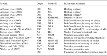
How to estimate? Nevertheless, given the very different dimensionality of the agent-based models, the econometric techniques involved also vary. Table 3 lists a number of studies related to calibration or estimation work. Estimation methods are given in the third column of the table. The three major estimation methods, namely, the method of moments, MLE, and LS, or their variants, are all involved. In addition to these standard methods, non-standard methods, such as GAs, are also used.
Estimation methods of ACF Models

ACF = agent-based computational finance.
The full meaning of the acronyms under ‘Origin’ are available in the Appendix. Here, we only provide the full name of those under ‘Methods’. ML stands for Maximum Likelihood, EMM for Efficient Method of Moments, NLS for Nonlinear Least Squares, OLS for Ordinal Least Squares, IEC for Interactive Evolutionary Computation, and MSM for Method of Simulated Moments.
What to estimate? To have an idea of the diversity shown in this table, it would be useful to first understand what we mean by estimating an agent-based financial model. The econometric construction of an agent-based financial model mainly contains two parts. The first part is directly related to the behavioral rules (parameters) of agents, for example, the reverting coefficient of fundamentalists, the extrapolating coefficient, the intensity of choice, the herding intensity, and the thresholds of rule switching. The second part is related to the external setting of the environment facing the agents, for example, the price adjustment speed (see the last column of Table 3).
4.1 How to estimate?
Direct estimation. The general idea of estimation is to derive the aggregation equation in which all these parameters are encapsulated. Then by applying appropriate statistical techniques to these equations one can derive the estimates of these parameters. Hence, if the aggregate equation happens to be a likelihood function, then the method involved is naturally the MLE method (Alfarano et al., Reference Alfarano, Lux and Wagner2005, Reference Alfarano, Lux and Wagner2006, Reference Alfarano, Lux and Wagner2007). If the aggregate equation happens to be a regression, then the employed method is LS (de Jong et al., Reference de Jong, Verschoor and Zwinkels2006; Boswijk et al., Reference Boswijk, Hommes and Manzan2007; Manzan & Westerhoff, Reference Manzan and Westerhoff2007).
Indirect estimation. However, for some classes of agent-based financial models, particularly those complex agent-based models reviewed in Section 2.2, it may not be easy to derive the aggregation equation in an analytical way, so that the direct application of econometric techniques is not feasible. Hence, an alternative approach is that, instead of deriving the aggregation analytically, the aggregation is derived via simulation, and the econometric steps are applied based on these simulated aggregations. Some estimation work shown in Table 3 belongs to this kind, which is also known as indirect estimation, to be distinguished, however, from the above-mentioned direct estimation. Examples of indirect estimation are Winker and Gilli (Reference Winker and Gilli2001), Gilli and Winker (Reference Gilli and Winker2003), Winker et al. (Reference Winker, Gilli and Jeleskovic2007), and Amilon (Reference Amilon2008). Since this approach is relatively new for agent-based economists, and can potentially be applied to a larger class of ACE models, we will give a brief review of this approach in Section 4.1.1.
4.1.1 Simulated-based estimation
Despite the progress observed in Section 4.1, agent-based models in general are very hard to estimate due to the lack of tractable criterion functions (likelihood functions, moments). Nevertheless, this problem is largely shared by many other economic or econometric modelsFootnote 15, and has received in-depth treatment during the last two decades, which has also inspired the development of entirely new procedures based on simulation, referred to as the simulation-based econometric methods Footnote 16. As we shall see later, these new proposed methods are very applicable and may dramatically open the empirical accessibility of agent-based models in the future.
Simulation-based econometric methods include the method of simulated moments (MSM), simulated maximum likelihood (SML), methods of simulated scores (MSS), efficient method of moments (EMM), and indirect inference. Some of these methods have already been applied to estimate agent-based models. For example, the MSM is used in Winker and Gilli (Reference Winker and Gilli2001), Gilli and Winker (Reference Gilli and Winker2003), and Winker et al. (Reference Winker, Gilli and Jeleskovic2007), whereas the EMM is used in Amilon (Reference Amilon2008).
4.1.2 Methods of simulated moments
The basic idea of simulated-based inference is to calibrate the parameter vector so that the properties of the simulated series resemble those of the observed data. Take MSM as an example. We first choose a vector of parameter values to generate the simulated time series by running the agent-based model with this chosen set of parameter values. We then compare some statistics (moments) of this simulated time series, the simulated moments, with those using real data, the sample moments. The difference between the two is used to form a distance function (the objective function). The MSM is purported to minimize the distance by searching over the entire parameter space.
Formally speaking, let X be a set of chosen statistics derived from the real data, X = (X 1, X 2, …, Xm), and Y be X's counterpart in the artificial data, Y = (Y 1, Y 2, …, Ym). In addition, let  be a distance function between X and Y. Then the indirect estimation of a set of parameters θ involves finding θ* such that

The indirect method, as claimed by Winker and Gilli (Reference Winker and Gilli2001), is general enough to be applied to other agent-based financial models, including SFI-like models. However, one of the main difficulties is solving Equation (17). Of course, an analytical solution in general is rarely available, and one has to rely on numerical approaches.
Example: Winker and Gilli (2001). Take Winker and Gilli (Reference Winker and Gilli2001) as an example. Winker and Gilli (Reference Winker and Gilli2001) attempted to estimate a version of the Kirman model (Kirman, Reference Kirman1991, Reference Kirman1993). There are two major parameters in this model, the self-conversion rate and the conviction rate, denoted by θ 1 and θ 2, respectively. To replicate the two characteristic features of financial time series, namely, fat tails and volatility clustering, their choice of X includes the following statistics: kurtosis and the first-order ARCH (AutoRegressive Conditional Heteroskedasticity) coefficient, which are denoted by X 1 and X 2. Then, given a specific choice of the distance function as shown below, the indirect estimator of θ is

Y 1 and Y 2 are the counterparts of X 1 and X 2 in the artificial data. They are not based on a single run of the Kirman model  , but on 10 000 runs. In other words, Y 1 and Y 2 are the averages taken over the 10 000 sample statistics derived from the corresponding 10 000 artificial time series. To solve the optimization problem posted in Equation (18), Winker and Gilli (Reference Winker and Gilli2001) and Gilli and Winker (Reference Gilli and Winker2003) suggested the use of the simplex method, combined with threshold accepting.
Practical issues of MSM. It can be seen from the previous illustration that the indirect estimation results,  , can depend on a number of choices, which include
1. the dimensionality of the target vector (X),
2. the statistics included in the target vector (X 1, X 2, …)
3. the parameters considered (θ)
4. the distance function (
 ),
5. the search algorithm used to solve global optimization,
6. the number of runs of the model
, or the sample size upon which Y is derived.
 ),
 , or the sample size upon which Y is derived.
This sensitivity may introduce a number of issues in the use of the indirect estimation approach. The first issue has to do with the selection of adequate statistics X. Winker et al. (Reference Winker, Gilli and Jeleskovic2007) proposed two criteria: robustness and powerfulness. The robustness criterion is involved because θ may be sensitive to the actual realization of X, say, x. If x is not stable over the entire sample, it would be less meaningful to anchor a specific  to the whole series. The powerfulness criterion requires the involved statistics to exhibit the potential to discriminate between alternative models and/or parameter constellations.
The second issue is the selection of the parameter vector (θ). While, in principle, all parameters involved in the agent-based model under study should be included, it is very difficult to do this in practice. This is mainly because the search space grows exponentially with the dimension of θ. Hence, this practical restriction allows us to estimate only a subset of θ = (θ 1,θ 2), say, θ 1, and the rest, θ 2, has to be fixed a priori.
4.1.3 Genetic algorithms
What seems to be interesting is that the estimation of agent-based models actually starts with the one involving the complex objective functions (Miller, Reference Miller1998; Ecemis et al., Reference Ecemis, Bonabeau and Ashburn2005; Midgley et al., Reference Midgley, Marks and Kunchamwar2007). A common feature shared by these papers is the use of GAs. Midgley et al. (Reference Midgley, Marks and Kunchamwar2007) provide a general framework for this approachFootnote 17. The idea is to use GAs to evolve the agent-based models so as to optimize the objective function.
Of all econometric agent-based models, Ecemis et al. (Reference Ecemis, Bonabeau and Ashburn2005) is probably the one with the most general objective function. They consider the possibility that the objective function for a model cannot be practically formulated mathematically, and is highly qualitative. In general, how well the model reproduces the data qualitatively can be no different from the appraisal of a performing art. A few statistics or moments may not be able to capture all we want. When it is hard to articulate the objective function, which reveals what we really want, then an automatic evaluation of a model becomes infeasible. An alternative solution is to allow financial experts to directly evaluate the models based on their expertise.
4.2 What to estimate?
The next issue concerns what is estimated. This issue is as important as the issue of how to estimate, because it is what was estimated that helps us to gain more insights from agent-based financial models. In particular, many agent-based financial models emphasize the contribution of learning or social interaction to the asset price dynamics. It would then be desirable to know whether these effects are empirically significant. In the last column of Table 3, we list the key parameters estimated by each model.
4.2.1 ANT model
We start with the ANT model, proposed by Kirman (Reference Kirman1991, Reference Kirman1993), since this is the first agent-based financial model being estimated. The ANT model is a two-type model consisting of fundamentalists and chartists. Let q 1 and q 2 be the fraction of fundamentalists and chartists, respectively, q 1 = 1 − q 2. There are two key parameters in the ANT model. Let θ 1 and θ 2 be the mutation rate (the self-conversion rate) and the conviction rateFootnote 18. It is found that when the following inequality, Equation (19), holds, the market fraction q 1,t spends little time around the value of one-half but a great deal of time at the extremes, that is, nearly zero or one.

where N is the number of agents. The ANT model has been estimated three times in the literature (Winker & Gilli, Reference Winker and Gilli2001; Gilli & Winker, Reference Gilli and Winker2003; Winker et al., Reference Winker, Gilli and Jeleskovic2007). Using the indirect estimation mentioned in Section 4.1.1, Winker and Gilli (Reference Winker and Gilli2001) found

Gilli and Winker (Reference Gilli and Winker2003) considered a three-parameter ANT model: in addition to the two parameters above, they also included a parameter related to noise distributionFootnote 19. Equation (20) is again sustained. Based on Kirman (Reference Kirman1991), this finding indicates that there is significant switching between fundamentalists and chartists; sometimes the market is dominated by fundamentalists, and sometimes by chartistsFootnote 20. Winker et al. (Reference Winker, Gilli and Jeleskovic2007) moved back to the two-parameter ANT model, but by using an objective function, which is closer in spirit to the simulated method of moments. This time they also gave a significance test of the model being estimated via a bootstrap methodFootnote 21. Whether the relation (20) holds was no longer discussed explicitly, even though the model with the parameter vectors considered was rejected.
4.2.2 Lux's interactive agent hypothesis model
As discussed in Section 2.1.3, there are two determinants that govern the switching behavior in Lux's IAH model, that is, herding and the profit differential. When it comes to the estimation of the Lux model, only the simple version with herding was estimated in Alfarano et al. (Reference Alfarano, Lux and Wagner2005, Reference Alfarano, Lux and Wagner2006, Reference Alfarano, Lux and Wagner2007), whereas the more general version with both determinants was estimated in Winker et al. (Reference Winker, Gilli and Jeleskovic2007). It should be noted that although herding is a common switching setting in the ANT model and the Lux model, the magnitudes of the parameters play different roles in these two models. In the ANT model, the switching parameters must satisfy Equation (19) in order to generate a bimodal distribution, which replicates the original observation in entomology and this is also an indication of significant switching behavior. In the Lux model, herding is presented only in the sense of following the majority (micro-level) but is not necessarily a strongly dominated group all the time (macro-level). In addition, the significance of switching behavior can be estimated and inferred directly (Alfarano et al., Reference Alfarano, Lux and Wagner2005, Reference Alfarano, Lux and Wagner2006, Reference Alfarano, Lux and Wagner2007) or indirectly (Winker et al., Reference Winker, Gilli and Jeleskovic2007).
Alfarano, Lux, and Wagner (2005, 2006, 2007). A two-type Lux model with only a herding mechanism in the transition rate function was estimated by Alfarano et al. (Reference Alfarano, Lux and Wagner2005, Reference Alfarano, Lux and Wagner2006, Reference Alfarano, Lux and Wagner2007)Footnote 22. Similarly to Kirman (Reference Kirman1991, Reference Kirman1993), they introduced the parameters of an idiosyncratic propensity a and herding tendency b, with the difference that the idiosyncratic propensity to switch to the other strategy is asymmetric, and is denoted as a 1 and a 2, which is different from the common probability of self-conversion that implies a 1 = a 2 in Kirman's setting. The major parameters to be estimated in this model are ε 1 and ε 2 where  . Let z be the fraction of noise traders. It can be shown that ε 1 and ε 2 determine the average percentage of noise traders in the market:

They can characterize the market by a dominance of fundamentalists’ or noise traders’ activity through estimating the magnitude of switching parameters. Although there is an exception in the Australian stock market (Alfarano et al., Reference Alfarano, Lux and Wagner2006), the noise traders’ dominance in stock markets, that is,  , seems a robust result over almost each individual stock in Japan and Germany (Alfarano et al., Reference Alfarano, Lux and Wagner2005, Reference Alfarano, Lux and Wagner2007). Furthermore, the model with an extreme switching tendency,
 , implying extreme dominance of noise traders, cannot be rejected for a large number of cases in Japan.
Winker, Gilli, and Jeleskovic (2007). Another empirical estimation of the Lux model was performed by Winker et al. (Reference Winker, Gilli and Jeleskovic2007), based on the indirect estimation mentioned in Section 4.1.1. They estimated a three-type Lux model, including fundamentalists and two types of chartists, that is, optimists and pessimists. Unlike Alfarano et al. (Reference Alfarano, Lux and Wagner2005, Reference Alfarano, Lux and Wagner2006, Reference Alfarano, Lux and Wagner2007), the complexity of this version of the Lux model makes the selection of the parameters being estimated no longer so trivial. They only choose three parameters: the general frequency of the revision of opinion between optimists and pessimists, the general frequency of the revision of opinion between fundamentalists and chartists, and the reaction strength of the fundamentalists’ excess demand. A significance test of the model being estimated is also performed via the bootstrap method. As it turns out, the Lux model was rejected, similar to the rejection of the ANT model, and the estimates of the parameters were not discussed in this work.
4.2.3 Adaptive belief systems model
Unlike Kirman (Reference Kirman1991), the ABS model (Brock & Hommes, Reference Brock and Hommes1998) leaves the forecasting rules, in parametric forms, that are employed by agents to be determined by the data. In some settings, the estimation of these coefficients can be interesting. For example, in the simple fundamentalist-and-chartist model, the expectations of fundamentalists and chartists can be described as in Equations (2) and (3). The parameters to estimate are the reverting coefficients (αf) and (αc). As discussed in Section 2.1.1, the magnitude of αf measures the speed with which the fundamentalists expect the price to return to the fundamental price, whereas the magnitude of αc expresses the degree to which chartists expect the past to change in the future. Together with the intensity of choice (λ) in the switching model (Equation (7)), there are at least three economically meaningful parameters to be estimated, namely,

There are at least two empirical estimations of the ABS model (Boswijk et al. Reference Boswijk, Hommes and Manzan2007; Amilon, Reference Amilon2008).
Boswijk, Hommes, and Manzan (2007). Boswijk et al. (Reference Boswijk, Hommes and Manzan2007) estimated a three-parameter ABS model using yearly S&P 500 data from 1871 to 2003. The three parameters are the ones described in (22)Footnote 23. Their estimated θ 1 and θ 2 are significantly different from zero, and are also correct in terms of their magnitude, which justifies the co-existence of the mean-reverting belief and the trend-following belief. Their estimation also provides us with a time series of the market fraction, which again shows that  (the fraction of fundamentalists) can swing from zero to one, with a mean of around 0.5. This result is similar to the empirical results from the ANT model (Winker & Gilli, Reference Winker and Gilli2001; Gilli & Winker, Reference Gilli and Winker2003), and lends support to the market fraction hypothesis or evolving fraction hypothesis. What may differ from the ANT model is the learning behavior of agents. In the ABS model, the learning behavior is mainly captured by the parameter, intensity of choice, which is, however, not found to be significant in Boswijk et al. (Reference Boswijk, Hommes and Manzan2007).
Market fraction hypothesis (MFH). The market fraction hypothesis basically says that the financial time series observed can be described in terms of switching between different types of agents, each with either different beliefs or different trading rules. In sum, the market dynamics is well explained by the evolving fractions of different types of financial agents. This is one of the most fundamental implications obtained from ACF models. Using yearly S&P 500 data from 1871 to 2003, Boswijk et al. (Reference Boswijk, Hommes and Manzan2007) found that the two types of investors, fundamentalists and chartists, coexist and their fractions exhibit considerable fluctuations over time. Before the 1990s, only occasionally did chartists (trend-chasers) dominate, and this dominance never persisted for more than 2 consecutive years. However, in the late 1990s the fraction of them increased to close to one and persisted for a number of years. The persistently high fraction of chartists in the market contributed to an explosive growth of the stock market, and resulted in annual returns of more than 20% for 4 consecutive years. Similar findings regarding the considerable fluctuations in the fractions are also obtained in other different agent-based financial markets, including foreign exchange markets.
Amilon (2008). Amilon (Reference Amilon2008) estimated both a two-type and a three-type ABS model. For the latter, in addition to the behavioral rules (2) and (3), he also introduced contrarians into the model with their behavioral rule described in Equation (4). Furthermore, both the behavorial rules (3) and (4) are extended to incorporate a memory parameter, βc and βco, respectively, as in Equations (5) and (6). Therefore, in addition to the mean-reverting and extrapolation coefficients, the memory of both chartists and contrarians becomes another parameter to estimate. This, with other extensions, actually leads to a 9-parameter two-type ABS model and a 14-parameter three-type ABS modelFootnote 24.
It is found that all major behavorial coefficients in the two-type model are insignificant, whereas they, including the intensity of choice, are all significant in the three-type modelFootnote 25. Nevertheless, most of the parameters are right in terms of magnitude. In particular, in the three-type model, all three heterogeneous beliefs are successfully identified. What, however, is interesting is that the swing between different types of agents is restricted only to the chartists (momentum traders) and contrarians. The fraction of fundamentalists is effectively zero. In other words, the inclusion of contrarians makes it hard for fundamentalists to survive. It, therefore, makes us wonder whether these three types of agents are redundant and whether either a fundamentalist–chartist model or a trend-chaser and contrarian model would suffice to do the job.
4.2.4 Santa Fe Institute-like models
AGEDASI TOF. AGEDASI TOF, standing for A GEnetic-algorithmic Double Auction SImulation in the TOkyo Foreign exchange market, was initially proposed by Izumi and Okatsu (Reference Izumi and Okatsu1996) and Izumi and Ueda (Reference Izumi and Ueda1999). It follows an AA design. Like the SF-ASM, agents (artificial dealers) make their investment decisions (buying or selling foreign currency) based on their forecasts of the investment return and risk. To forecast investment return, each artificial dealer will refer to a number of economic and political variables, such as gross domestic product (GDP), the consumer price index (CPI), interest rates, money supply, etc. However, the exact relationships between the foreign exchange rate and these variables are unknown, and have to be exploited.
Therefore, in the vein of the SF-ASM, AGEDASI TOF also used GAs to model agents’ learning behavior (forecasting). GA helps agents to decide the magnitudes and signs assigned to each variable. Up to this point, there is nothing significantly different from the SFI model. However, AGEDASI TOF allows its artificial dealers to get access to external data, that is, data from the real world, to forecast the exchange rate, which means the data, such as GDP, CPI, etc. are all real. This modeling strategy is essentially equivalent to a direct estimation of the behavioral rules (forecasting models) of agents, and then uses the estimated rules of each agent to generate the aggregate behavior (exchange rate).
The system has been shown to have a better forecasting performance than benchmarks, such as the random walk. In particular, it has a good performance in long-term forecasting; it can also be used to forecast the probability of a particular event, such as bubbles and crashes. For example, the model gives a probability of 42% of observing a bubble in the Tokyo foreign exchange market in the years 1989–1991.
From an estimation viewpoint, the econometric approach exemplified by AGEDASI TOF is not a real econometric approach but a computational intelligence approach in a bottom-up style. This direct bottom-up estimation approach is more intuitive and applicable to the SF-type models; nonetheless, whether it can satisfy econometrics standards requires further study.
4.3 Forecasts with agent-based financial models
It has been long asked, instead of just replicating or growing the stylized facts, whether the agent-based model can be a useful tool for forecasting. In other words, in addition to providing a bottom-up mechanism to explain the stylized fact as an emergent outcome, interest is further drawn to the prediction power of the same mechanism. The recent research trend seems to indicate that one can be cautiously optimistic about this possibility. This is particularly so given the recent contribution of de Jong et al. (Reference de Jong, Verschoor and Zwinkels2006) and Manzan and Westerhoff (Reference Manzan and Westerhoff2007)Footnote 26.
de Jong, Verschoor, and Zwinkels (2006). Following standard econometric forecasting procedures, first of all, de Jong et al., (Reference de Jong, Verschoor and Zwinkels2006) estimated two versions of a three-type ABS model, one with a switching mechanism and one without it. The first two types of agent are the usual fundamentalists and chartists (Equations (2) and (3), or, in general, Equation (5)), but, for the third type, they considered a different kind of chartist, called the MA-chartist, whose forecasting rule is based on the difference between a long-term moving average and a short-term moving average:

where  refers to the moving averages with a window length of L and
 refers to a window length of S (L > S). One can consider the MA-chartist as a kind of fundamentalist if the fundamental price
 in Equation (2) is replaced by the long-term moving average
 .
de Jong et al. (Reference de Jong, Verschoor and Zwinkels2006) estimated this three-type model using data from eight foreign exchange markets. They found evidence supporting heterogeneity in the behavior of agents, but not supporting a significant intensity of choice. The latter with a similar finding in Boswijk et al. (Reference Boswijk, Hommes and Manzan2007) and Amilon (Reference Amilon2008) (the three-type case) really casts doubt on the essence of the ABS, namely, the sensitivity to profit or performance differentials. The estimated model is then applied to forecast the future exchange rate with different horizons. Using the Diebold–Mariano test (Diebold and Mariano Reference Diebold and Mariano1995), they were able to demonstrate that the three-type model can outperform the random walk in most markets with various settings of different horizons or criteria. Nevertheless, this superiority in forecasting may not be taken seriously since the usual distinction between the training sample and test (unseen) sample is not made in their study.
Manzan and Westerhoff (2007). In a similar vein, Manzan and Westerhoff (Reference Manzan and Westerhoff2007) estimated the two-type models with and without switching using monthly exchange rate data. The adaptive behavior in this paper is not driven by the profit differential or herding, but it is an exogenous threshold value that governs the sentiment of the chartist. From the econometrics perspective, they actually incorporated a threshold autoregressive structure, and hence nonlinearity, into the model. On the other hand, since this kind of threshold mechanism itself implies an immediate switch once the state variable passes the threshold, it is equivalent to having an infinitely large intensity of choice in the binary-choice model (Equation (8)). The estimation results and nonlinearity tests are in favor of the model with a switch. They then dynamically estimated the proposed two-type model with a rolling window and made the one-step-ahead forecast accordingly. Using the Diebold–Mariano test, they showed that the two-type model can outperform the random walk model for two of six currencies.
In not only using the Diebold–Mariano test as a predictability test, Manzan and Westerhoff (Reference Manzan and Westerhoff2007) also raised a question about its test power. They treated their agent-based model as a real-data-generating process, which contains both a linear adjustment process (the fundamentalists) and a nonlinear switching mechanism (the chartists). These two components can be captured by the estimation methods proposed by Mark (Reference Mark1995) and Diebold and Nason (Reference Diebold and Nason1990). It should be expected that the nice in-sample estimation results could carry over into the out-of-sample forecasting for simulated time series and lead to better forecasting accuracy over the random walk. However, the Diebold–Mariano test cannot well endorse such an improvement, which means that its test power is quite low.
Prospectives. Even though the forecasting capability of the agent-based model has not been consolidated, there are reasons to be optimistic. First, the bottom-up mechanism in the agent-based model behaves as a pool of many agents’ forecasting, which is very similar to what is known as the prediction markets or information markets. Second, the emergent behavior (the aggregate behavior) also behaves as a combination of different forecasts, which is, therefore, a kind of combined forecast. In the literature, evidence of the superiority of the prediction markets over the poll and other forecasts and evidence of the superiority of the combined forecast over simple forecasts already exists, while not necessarily overwhelmingly. Therefore, it is anticipated that the agent-based model under a suitable construction process may lead to some desirable outcomes.
5 Emerging econometrics with agent-based computational econometrics
Most empirically based ACE models only consider how econometrics can help to build or validate the ACE models. Few have explored whether the other way around may be equally interesting. In this section, we shall present some thoughts on the reverse direction, that is, instead of an econometric foundation of ABE, an agent-based foundation of econometrics. In this regard, ACE can present challenges to econometrics.
5.1 Aggregation problems
Intuitively, ACE can help econometrics because it is a kind of the micro–macro approach. This micro–macro approach has been reviewed by Stoker (Reference Stoker1993) as an approach to address the aggregation problem. The ACE model, as a computational model, provides us with a greater flexibility to deal with various levels of aggregation over individuals. Unlike many other micro–macro models, it does not have to make very stringent assumptions regarding individual behavior in order to have a tractable aggregation. This advantage enables us to include more realistic behavioral aspects of individuals into the aggregation, such as learning and interactions. In the following, by using an agent-based consumption asset-pricing model (Chen et al., Reference Chen, Liao and Chou2008), we shall demonstrate how the ACE model can help solve the aggregation problem.
5.1.1 Estimation using the individual data
We start with an individual i's consumption Euler equation as follows:

where  is the consumption growth at time t,

In the consumption-based capital asset pricing model (CAPM),  , under suitable assumptions, is also known as the elasticity of intertemporal substitution (EIS).
 is the real return on the asset at t,
 is a constant, and
 is the residual variable. Notice that the heterogeneity of individuals in terms of
 makes Equation (24) also heterogeneous among agents. Furthermore, the heterogeneity in terms of investment behavior also makes the rates of return rt facing agents heterogeneous, which are denoted by
 in Equation (24).
The return facing each individual is determined by his or her chosen portfolio  , and can be calculated as follows:

where

and

pm,t is the price of the asset m at time t, and wm,t is the dividend paid for the asset m at time t.
To estimate the coefficients  , we may consider the set of l individual equations as one giant equation, and estimate the l
 s altogether. This is the familiar seemingly unrelated regression estimation (SURE). SURE can be useful when the error terms
 of each equation in (24) are related. In this case, the shock affecting the consumption of one agent may spill over and affect the consumption of the other agents. Hence, estimating these equations as a set, using a single large equation, should improve efficiency. To apply SURE, we rewrite the set of equations (24) into a single equation as (29):

where

5.1.2 Estimation using the aggregate data
The early econometric work on the estimation of the EIS mainly used only aggregate data (Hall, Reference Hall1988). In this section, we also estimate the ψ based on the aggregate data:

Equation (30) is the Euler consumption equation that is based on the assumption of treating the whole economy as a single representative agent. This version is the one frequently used in macroeconometrics. Δct and rt are the corresponding aggregate variables of consumption and returns.
5.1.3 Micro–macro relation
One way to formulate the aggregation problem has to do with the relationship between  (the individual estimates) based on Equation (29) and
 (the aggregate estimate) based on Equation (30). For example, if the
 are all identical, say ψ i = 1, ∀i, we can have
 . Furthermore, if we are informed of the distribution of the ψ i, what can we further say about
 ? This is the kind of aggregation problem which has been generally surveyed in Stoker (Reference Stoker1993). Stoker (Reference Stoker1993) detailed a solution called the micro-macro approach. This approach models the comparability of individual behavioral patterns and aggregate data patterns, removing any mystery induced by the one-sided focus of studying aggregate data alone or individual data alone. The approach has been further pursued recently by Gallegati et al. (Reference Gallegati, Palestrini, Delli Gatti and Scalas2006).
Chen et al. (Reference Chen, Huang and Wang2008) use an agent-based consumption-based CAPM model to simulate all artificial time series required by the individual Euler equation, and they estimate the individuals’ EIS coefficients through Equation (29). Then they also run the aggregate Euler equations (30) by using the aggregate data. What surprises them is that the two estimates can be quite distinct. Given the assumption that ψ i = 1 (∀i), none of the individual and aggregate Euler equations can recover this behavioral parameter in a reasonably close range. Most estimated individual ψ is are around 0.3, whereas the estimated aggregate ψ is close to zero.
Elasticity puzzle: real or spurious? If we further assume EIS to be the reciprocal of the coefficient of risk aversion, then this result implies an unreasonably high risk aversion. The latter conundrum is also known as the elasticity puzzle (Neely et al., Reference Neely, Roy and Whiteman2001). What, therefore, is shown in Chen et al. (Reference Chen, Huang and Wang2008) is that if we follow standard econometric practice with the representative agent framework, then we can easily obtain this purely spurious result simply because of the negligence of aggregation over interacting heterogeneous boundedly rational agents. This phenomenon has been also well noticed by Delli Gatti et al. (Reference Delli Gatti, Gaffeo, Gallegati, Giulioni, Kirman, Palestrini and Russo2007):
‘If agents are heterogeneous, some standard procedures (e.g. cointegration, Granger-causality, impulse-response functions of structural VARs) lose their significance. Moreover, neglecting heterogeneity in aggregate equations generates spurious evidence of dynamic structure’ (Delli Gatti et al., Reference Delli Gatti, Gaffeo, Gallegati, Giulioni, Kirman, Palestrini and Russo2007).
ACE as a data-generation mechanism (DGM). Hence, by using ACE in the model as a DGM, we can examine the behavior of various econometric tests, particularly, those macroeconometric tests, to see whether they actually behave well when the data are indeed the aggregation over interacting heterogeneous bounded rational individuals. Since the ACE model can easily accommodate different kinds of learning algorithms and interaction mechanisms, this prompts us to perform a sensitivity analysis to see whether the ideal behavior of the standard econometrics can be robust to different micro-underpinnings.
5.2 Imperfect data
ACE can help to test some hypotheses, which are very difficult to test on the real data. This can happen when the respective real data are not easily available. One example concerns agents’ expectations. In the literature on sunspot equilibria in macroeconomics, there is a concern among macroeconomists whether something that is totally extrinsic to a system can eventually have effects on the operation to the system, simply because agents ‘naively’ believe so. Nevertheless, it is widely shared among macroeconometricians that the direct empirical test of the existence of sunspot beliefs and sunspot equilibria can be rather difficult due to the lack of observed data. Some recent progress in this area has been made using the experimental approach (Duffy & Fisher, Reference Duffy and Fisher2005), but ACE can provide an alternative way out of the empirical difficulty (Chen et al., Reference Chen, Liao and Chou2008).
ACE models can directly control the interactions among agents as well as their learning processes, and indirectly define the transmission process of sunspots. Of course, it is hard to know whether the real counterpart is the same or similar to the one used in a specific ACE model, but at least we know what the setting is and we can change the setting. This specific setting is equivalent to the assumption of a theorem, and we can then use standard econometric tests to examine whether belief matters with respect to different assumptions.
6 Concluding remarks
This paper provides a first review of the ACE models from an econometric viewpoint. Given the fast growth of both financial econometrics and agent-based finance, this paper, in many ways, serves only as a beginning and is by no means exhaustive.
First, the list of stylized facts is not exhaustive. We believe that the exploration of various financial data that were hardly available before will soon contribute to the lengthening of the list of stylized facts. Actually one area that we do not cover well concerns the data on the order book and the recent empirical findings of the order book that have triggered another wave of the development of ACF models. This is definitely a space, which we should fill in a future study.
Second, the standpoints by which we examine and differentiate various ACF models are also limited. We focus mainly on the behavioral rules of financial agents. This very suggestive taxonomy of the literature enables us able to see the minimum condition required to replicate the stylized facts in terms of the heterogeneity and complexity of behavioral rules. Needless to say, there are other ingredients, which deserve our further distinctions. The design of a network of interactions is an example. While most ACF models do implicitly assume a network for interactions (Kirman, Reference Kirman1991; Cont & Bouchaud, Reference Cont and Bouchaud2000; Iori, Reference Iori2002), work on the explicit modeling of interactions (Zovko & Farmer, Reference Zovko and Farmer2007; Hein et al., Reference Hein, Schwind and Spiwoks2008) is one area neglected in this survey. Therefore, the extent to which social networks can contribute to the understanding of stylized facts is also a direction for the future. Other examples include risk preferences (Shimokawa et al., Reference Shimokawa, Suzuki and Misawa2007), asynchronous updating (Boswijk et al., Reference Boswijk, Hommes and Manzan2007), information asymmetry (Suominen, Reference Suominen2001), and, finally, institutional constraints (Farmer et al., Reference Farmer, Patelli and Zovko2005).
Despite this incompleteness, it is found that the models with simple heterogeneity and simple rules (few-type models), in particular the variations of the fundamentalist–chartist model, are sufficient to replicate a number of stylized facts. A complex extension of this model may gain additional explanatory power, but so far this power has not been well exploited. In addition, the simple model makes later econometric estimation much more feasible.
Econometric estimation of agent-based financial market models is an ambitious task. In principle one can identify various details of agents, such as their beliefs, memory, intensity of choice, risk perceptions, and risk aversions, etc. It may also help us to infer the underlying fitness function, for example, profits vs. risk-adjusted profits, from the data. For the few-type model, one can further discover the evolving market fractions so as to track the mood of the market. Nevertheless, before we reap the fruits of these models, there is still a long way to go. So far, we have not been assured that these agent-based financial market models are econometrically significant, and the estimates are stable. One of the difficulties in front of us is how to effectively tackle the numerical aspects of the estimation of a complex objective function involving a large number of parameters.
However, the value of agent-based models should not be restricted to just replication or validation. This is particularly so when the econometrics to support quality validation is still lacking. Section 5 suggests that treating agent-based models as theoretical models, which behave as many other stochastic simulation models can help us to examine the power of the established econometric tests. This function can be most valuable when the environment is filled with various degrees of tainted or missing data. The paper therefore ends up with the message that the agent-based foundation of econometrics is the next stage to move toward.
Acknowledgments
An early version of the paper was presented at the Econophysics Colloquium 2008, August 28–30, 2008, at the University of Kiel, and also at the International Workshop on Nonlinear Economic Dynamics and Financial Market Modelling, October 9–10, 2008, at Peking University. Comments from participants such as Thomas Lux, Carr Hommes, Carl Chiarella, Tony He, and Duo Wang are all gratefully acknowledged. This final version has further benefited from the painstaking review of an anonymous referee and the guest editors of this special issue, Robert Marks and Nick Vriend. The NSC grants 95-2415-H-004-002-MY3 and 98-2410-H-004-045-MY3 are also greatly acknowledged.
Appendix A: Taxonomy of agent-based computational finance models and stylized facts explained
The appendix gives summary tables (Tables 4–7) of each of 50 agent-based computational finance (ACF) models surveyed in this article, including the stylized facts replicated or explained by each of them. In the second column of each table, we also indicate the intellectual origin or ingredients of each model. The most often seen ones are those that have been surveyed in Section 2, but there are also a few that are new here. The names of the origin are given in an acronym. Here, we list these acronyms with their full names. Some of the names given here are very suggestive.
Two-type designs and the stylized facts explained

Three-type designs and the stylized facts explained
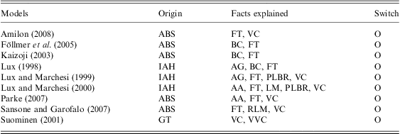
Many types models: stylized facts explained
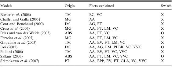
Autonomous-agent designs: stylized facts explained
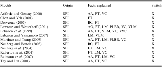
SFI = Santa Fe Institute.
1. ABS: Adaptive belief systems
2. ANT: Ant
3. IM: Ising model
4. IAH: Interactive agent hypothesis
5. GT: Game theory
6. MG: Minority games
7. MS: Microscopic simulation
8. PT: Prospect-theory-based model
9. TM: Threshold model
 . The third parameter considered by Gilli and Winker (
 is not available from this estimation. The estimation only gives us
 and
 , which allows us to simulate many equally likely series
 . Hence, we are not able to answer the question: between 1991 to 2000, when is the market dominated by fundamentalists and when is it dominated by chartists?