INTRODUCTION
Since laser is introduced in 1960, it has been applied extensively in such fields as weaponry, remote sensing, spectroscopy studies (Abdallah et al., Reference Abdallah, Batani, Desai, Lucchini, Faenov, Pikuz, Magunov and Narayanan2007), adaptive optics, and medical uses (Svanberg et al., Reference Svanberg, Andersson-Engels, Cubeddu, Förster, Grätz, Herrlin, Hölzer, Kiernan, Klinteberg, Persson, Pifferi, Sjögren and Wahlström2000), among others (Korobkin et al., Reference Korobkin and Romanovsky1998; Fleury et al., Reference Fleury, Bouquet, Stehlé, Koenig, Batani, Benuzzi-Mounaix, Chièze, Grandjouan, Grenier, Hall, Henry, Lafon, Leygnac, Malka, Marchet, Merdji, Michaut and Thais2002; Wolowski et al., Reference Wolowski, Badziak, Czarnecka, Parys, Pisarek, Rosinski, Turan and Yerci2007; Zvorykin et al., Reference Zvorykin, Berthe, Boustie, Levchenko and Ustinovskii2008). In recent years, laser has been used to extend radio-frequency atmospheric communication to the optical-frequency band again. Free space laser optics communication (FSO) has some potential advantages than conventional radio-frequency communications, including high data rate, the low probability of detection, low weight, and volume, etc. Modulation of the laser signal by optical turbulence is a major factor for communication links that traverse atmospheric paths. Optical turbulence is an important atmospheric phenomenon that adversely affects optical wave propagation. It is brought about by fluctuations in the atmosphere's refractive index due to inhomogeneities in temperature and pressure caused by solar heating and wind. When laser light, which is simply one form of optical wave, propagates through the atmosphere, optical turbulence distorts the optical path and further induces fluctuations in its amplitude and phase (Andrews & Phillips, Reference Andrews and Phillips1998; Tatarskii, Reference Tatarskii1961, Reference Tatarskii1971; Chiba, Reference Chiba1971; Stadnik et al., Reference Stadnik, Statsenko, Yanilkin and Zhmailo1997; Bashurin et al., Reference Bashurin, Bashurov, Bogunenko, Bondarenko, Pletenev and Starodubtsev1997; Kucherenko et al., Reference Kucherenko, Pylaev, Murzakov, Belomestnih, Popov and Tyaktev2003; Chiravalle, Reference Chiravalle2006). These effects can severely influence the performance of free-space laser optics communication systems (Majumdar & Ricklin, Reference Majumdar and Ricklin2004; Han Oh et al., Reference Han Oh, Ricklin, Oh, Doss-Hammel and Eaton2004; Kazaura et al., Reference Kazaura, Omae, Suzuki and Matsumoto2006; Andrews et al., Reference Andrews, Phillips and Yu1995).
In order to evaluate atmospheric turbulence-induced fluctuations in amplitude (intensity) and phase of laser beam and their effects on free-space laser optics communications, many experimental researches have been conducted. In early researches, intensity fluctuations attracted significant coverage from scientific community (Fried, Reference Fried1967; Fried et al., 1967; Parry, Reference Parry1981; Coles & Frehlich, Reference Coles and Frehlich1982; Churnside, Reference Churnside1991; Consortini et al., Reference Consortini, Cochetti, Churnside and Hill1993; Tunick, Reference Tunick2007a, Reference Tunick2007b) since it is much more difficult to measure phase fluctuations than intensity fluctuations in the optical-frequency band. However, recently, more and more experimental observations (Phillips et al., Reference Phillips, Andrews, Stryjewski, Griffis, Borbath, Galus, Burdge, Green, Kim, Stack, Harkrider, Wayne, Hand and Kiriazes2006; Rao et al., Reference Rao, Jiang and Ling1999; Silbaugh et al., Reference Silbaugh, Welsh and Roggemann1996; Ridley et al., Reference Ridley, Jakeman, Bryce and Walson2003; Giggenbach et al., Reference Giggenbach, David, Landrock, Pribil, Fischer, Buschner and Blaschke2002) concerning phase fluctuations were performed with the development of adaptive optics and high-resolution astronomic imaging technologies.
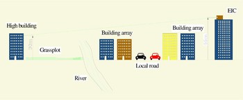
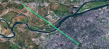
This paper presents an experiment that examines the angle-of-arrival (AOA) fluctuations of a laser beam propagating through a turbulent atmosphere over an 11.8 km urban path. The optical path is almost horizontal, which extends from the 9th floor (30 m above ground level) of a building in the Songbei district of Harbin to the rooftop of the electronic information center (55 m above ground level) at the National University Science Park of the Harbin Institute of Technology (see Figs. 1 and 2). The optical path traverses a complicated landscape, mainly including a piece of open grassplot, a river, several roads, and various building arrays. Non-uniform landscape leads to the complexity of the microclimate along the optical path and further produces an effect on the measured data. Besides, other factors, e.g., vibration of the buildings and temperature gradients, can also affect the experimental results.
(Color online) A schematic of the optical path.

(Color online) An aerial photograph of the optical path (data from maps. Google.com) (Jiang et al., Reference Jiang, Ma, Tan, Yu and Du2008).

Here, it should be noted that optical intensity data are also collected simultaneously to examine atmospheric turbulence-induced optical intensity fluctuations in this experiment, and the corresponding results have been reported in another paper (Jiang et al., Reference Jiang, Ma, Tan, Yu and Du2008).
EXPERIMENTAL SETUP
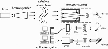
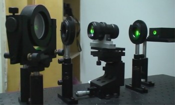
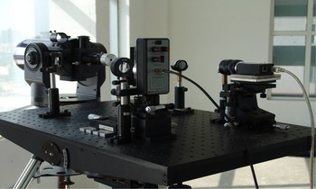
Figure 3 shows the schematic diagram of this experiment. The transmitter system, which is composed of a laser source, an expander, and a reflector, is mounted on a three-dimensional (700 mm × 450 mm) adjustable optical bench that is setup inside a room of a building (see Fig. 4). The laser source outputs a coherent optical beam with the wavelength of 0.532 µm and the adjustable output power from 20 mw to 100 mw, in order to assure that the experiment can still be carried out in some bad weather conditions. The expander is utilized to compress the initial beam divergence of 1.3 mrad to 0.25 mrad (4 mm input diameter and 24 mm output diameter). As a result, the laser beam spot has a diameter of about 3–4 m at the receiving plane. The reflector is used to adjust the transmitting direction of the laser beam conveniently.
A schematic diagram of this experiment.

(Color online) Photograph of the transmitting optics for this experiment.

The receiver system is situated on the rooftop of the electronic information center. The receiver antenna is a Cassegrain telescope. The diameter of the telescope is 127 mm and its magnification is 47.5. A splitter with the transmission and reflection ratio of 50/50 at 0.532 µm behind the telescope is utilized to split the output of the telescope into two beams: One is focused on a pin photo-detector (PIN) through a lens (f = 78.2 mm) to measure optical intensity fluctuations; the other is focused on a charge-coupled device (CCD) by its own lens (f = 50 mm) to obtain the experimental data used to calculate the AOA. Two 0.532 µm filters are placed in front of PIN and CCD, respectively, to eliminate the influence of background light. The attenuator is placed between the splitter and the filter (in front of CCD) to prevent CCD from power saturation. The telescope is installed on a tripod and other equipments are mounted on another three-dimensional adjustable optical bench (see Fig. 5).
(Color online) Photograph of the receiving optics and the three-dimensional adjustable bench for this experiment.

A computer connected to the CCD is used to calculate the centroid coordinate of CCD image, from which the AOA can be determined (Giggenbach et al., Reference Giggenbach, David, Landrock, Pribil, Fischer, Buschner and Blaschke2002). The image is sampled at the rate of 1000 Hz. During the measurement, the attenuator, and the exposal time of CCD are adjusted, respectively, to prevent the received optical intensity from overstepping the dynamic range of CCD. However, there are still occasional saturations due to urban turbulence complexity, and the smaller dynamic range of CCD, which can also influence the experimental results.
A temperature and humidity recorder is used to measure the air temperature and relative humidity every 3 min and a wind velocity recorder is also used to record the wind speed at the receiving end in order to obtain corresponding climate characteristics.
DATA ANALYSIS
The experiment is carried out from October 2006 to the end of the year of 2007, lasting more than one year. A typical experimental data set is chosen to analyze the characteristics of AOA fluctuations, which is mainly composed of four data trials collected during spring, summer, autumn, and winter, respectively. The data selection is mainly based on two criterions: One is whether there are more pixels on the CCD image; the other is whether there are no or less saturation pixels. The first criterion is chosen based on the consideration that more pixels can calculate more correctly the centroid coordinate of CCD image. The second criterion is chosen based on the consideration that less saturation pixels can result in less error induced by the saturation of the CCD. The variance of fluctuations, power spectrum, probability density function, and Fried coherence length were calculated for each chosen data trial, respectively.
Fluctuations Variance
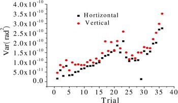
Table 1 summarizes the variances of AOA fluctuations, the date, and the microclimate condition for each trial. Note that besides the total variance, the variances in the vertical and horizontal directions are also calculated, respectively. As it is shown in Table 1, the variance in the vertical direction is larger than that in the horizontal direction for each trial. More data are also analyzed to further investigate this difference of AOA fluctuations in these two directions, totally including 36 trials, and the results are plotted in Figure 6. As it is shown in Figure 6, the results are similar to T1–T4. So it can be concluded that the variance of AOA fluctuations in the vertical direction is larger than that in the horizontal direction for near-horizontal laser beam propagation in the atmosphere. We consider that the result is introduced by the difference between the atmospheric turbulences in the vertical and horizontal directions due to gravity (Vernin, Reference Vernin, Tatarskii, Ishimaru and Zavorotny1992).
(Color online) The variances in the vertical and horizontal directions for 36 trials.

Variances, Fried coherence lengths, and microclimate characteristics for the experimental data set

Probability Density Function
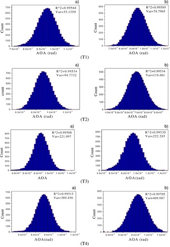
Usually, it is assumed that probability distribution of AOA should be normal (Giggenbach et al., Reference Giggenbach, David, Landrock, Pribil, Fischer, Buschner and Blaschke2002). Histograms for each trial in Table 1 and the fitting curves are shown in Figure 7. Note that histograms in the horizontal (1) and vertical (2) directions for each trial are also calculated, respectively. The variances and normal regression coefficients, R 2, are labeled on each graph. Here, the variance describes the fluctuations intensity of AOA, while R 2 (0 < R 2 < 1) stands for the related coefficient. The histograms match the fitting curves better if R 2 is more close to 1. The definition of R 2 may refer to Section 3.1 in Jiang et al. (Reference Jiang, Ma, Tan, Yu and Du2008).
(Color online) Histograms of AOA in the horizontal (a) and vertical (b) directions, and normal fitting curves (red lines) for trials T1, T2, T3, and T4.

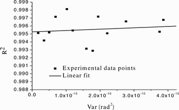
As it is shown in Figure 7, the histogram matches the normal fitting curve very well for each graph and R 2 are all above the level of 0.995. Other data trials are also analyzed and the results are similar to T1–T4. Their R 2 are plotted in Figure 8, the abscissa axes of which indicates the variances in the vertical direction. The fitting line in Figure 8 is almost horizontal, which means R 2 does not vary for different variances. So it can be concluded that the normal (distribution) approximation is equally effective to trials with different variances. The experimental data in the horizontal direction are also analyzed, and the same conclusion can also be obtained (not shown).
R 2versus variances for trials.

Power Spectrum
Figure 9 shows the power spectra calculated for each trial in Table 1. It is noted that the power spectra in the horizontal (black line) and vertical (red line—color online) directions for each trial are also computed, respectively. The power spectrum in the horizontal direction is similar to that in the vertical direction for each trail and they have the same exponential power law dependence, while the power exponents for different trials are different. The power exponents for trials T1, T2, T3, and T4 are −4.5/3, −4.6/3, −3.5/3 and −3.8/3, respectively. More data trials are analyzed to examine the characteristics of the power spectrum. The results show that the power exponents are not constant for different trials. The power exponent varies in a broad range from −2.1/3 to −7.8/3 for all of the analyzed data trials.
Power spectra for trials T1 (a), T2 (b), T3 (c), and T4 (d), and power laws are annotated on each graph.

However, the theoretical investigation has shown that the power spectrum of AOA fluctuations follows the −8/3 power law (Clifford, Reference Clifford1971). The experimental results are different from the theoretical result for the power law value. In addition, the power-law values for all of the analyzed data trials are larger than the theoretical result, −8/3. It is very difficult to tell what makes the experimental results so different from the theoretical result. The reasons induced such results probably include the error of the detector, the complexity of the urban turbulence (Wang et al., Reference Wang, Fan, Wu, Zhan and Gong2000); the validity of the Kolmogrov model (Stribling et al., Reference Stribling, Welsh and Roggemann1995), the turbulence scale and boundary (Rao et al., Reference Rao, Wang, Liu and Gong1999; Golbraikh & Kopeika, Reference Golbraikh and Kopeika2004), and the model of optical wave (Rao & Gong, Reference Rao and Gong2002). All of these factors can produce an effect on the experimental results.
Finally, it should be emphasized that the power spectrum of AOA fluctuations is different from that of the intensity fluctuations (Jiang et al., Reference Jiang, Ma, Tan, Yu and Du2008) in this experiment. The power spectrum of AOA fluctuations has the same power-law dependence in the whole frequency range, while the power spectrum of intensity fluctuations is divided into the high-frequency spectrum and the low-frequency one, which have different power-law dependence.
Daily Variations Characteristics of Path-Averaged Values of C n2
Usually, the intensity of optical turbulence is described by the structure parameter of refractive index C n2. In this experiment, the daily variations characteristics of path-averaged values of C n2 are investigated based on the analysis of the experimental data of AOA. Path-averaged C n2 can be calculated from the variance of AOA by the following formula (Jiang et al., Reference Jiang, Ma, Tan, Yu and Du2008)

where σ α2 is the variance of AOA fluctuations, L = 11.8 km is the path length, and D = 127 mm is the diameter of the receiving aperture.
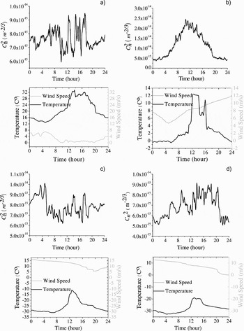
The trials are conducted on January 31, March 26, June 21, and December 15, 2007, respectively, and each trial lasts at least 24 hr. The 10 min average values of path-averaged C n2 are plotted in Figure 10 for these four trials.
Daily variation of optical turbulent intensity Cn 2 and meteorological data (a) at June 21; (b) at March 26; (c) at January 31, and (d) at December 15.

As it is shown in Figure 10, the daily variations characteristics of path-averaged optical turbulence intensity C n2 are more complicated than the results reported by Tunick (Reference Tunick2007a, Reference Tunick2007b). They do not appear a consistent regularity. We consider that this complexity is perhaps caused by worse inhomogeneity of the random field of refractive-index fluctuations over the long urban path.
Fried Coherence Length
For a Gaussian-beam wave, the wave structure function can be expressed as (Andrews & Phillips, Reference Andrews and Phillips1998)
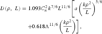
where L is the link distance, D is the diameter of the receiving aperture, and
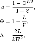
F (F ≈ L, if L is long enough) and W denote the receiver plane phase front radius of curvature and the beam radius, respectively. In our experiment, k and L are on the order of 107 and 104, respectively, the beam radius W is about 3–4 m, and D = 127 mm. Based on these parameters, the approximation of F ≈ L, a ≈ 1 and Λ ≈ 0 can be made, and Eq. (3) can be simplified to

According to the definition of Fried, coherence length given by Fried (Fried et al., Reference Fried, Mevers and Keister1967), the Fried coherence length for Gaussian-beam wave (used in this experiment) has the form:
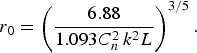
Using Eq. (1), the above formula can be expressed by the variance of AOA,
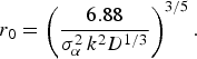
Since the variance of AOA has been calculated in this experiment, the Fried coherence length can be investigated by Eq. (6).
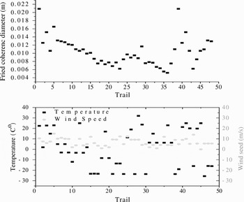
For the typical experimental data set in Table 1, the Fried coherence lengths are calculated, which also summarizes in Table 1. More data trials are also analyzed to further investigate the characteristics of Fried coherence lengths, totally including 48 trials, and the results are plotted in Figure 11. As it is shown in Figure 11, the Fried coherence length varies from 5 mm to 21 mm for all of the analyzed data trials.
The variances in the Fried coherence length and meteorological data for 48 trials.

Aperture Averaging
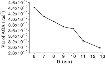
Usually, it is accepted that the fluctuations of AOA decreases with the increase of the receiving aperture, which is called the aperture averaging effect (Andrews & Phillips, Reference Andrews and Phillips1998). In this experiment, the variances of AOA are measured as the diameter of receiving aperture, taking all value ranging 60 mm to 127 mm with the step of 1 cm. As it is shown in Figure 12, the variances of AOA decrease with the increase of receiving aperture, which approves the aperture averaging effect.
Variance of AOA fluctuations versus the diameter of receiving aperture.

SUMMARY AND CONCLUSION
Experimental research is carried out to examine the characteristics behavior of AOA for a laser beam propagating through a turbulent atmosphere over an 11.8 km urban path. Data analysis is mainly based on a data set which is composed of four data trials collected during spring, summer, autumn, and winter, respectively. The results of the variance analysis show that the variance in the vertical direction is larger than that in the horizontal direction. Histogram of frequency count is also made for each trial. Normal distributions are proved to be nice approximations for different variance trials. Power spectra are plotted and the power law appears to vary in a broad range from −2.1/3 to −7.8/3. Fried coherence length is also calculated based on the variance of AOA and its value varies from 5 mm to 21 mm for all of the analyzed data trials. In addition, the daily variation of path-averaged optical turbulence intensity C n2 is investigated based on the experimental data of four days, and the results show that the daily variation of path-averaged C n2 is complicated and does not have a consistent law. Finally, the aperture averaging theory is confirmed based on the analysis of experimental data measured with different apertures. This work can benefit the research of laser atmospheric transmission and the free-space laser optics communication system design.
ACKNOWLEDGMENT
This work is supported by the program of excellent team in Harbin Institute of Technology.