Introduction
Spatial heterogeneity in resource availability leads to complex patterns of tree species composition in tropical forests. Most tropical tree species are spatially aggregated at the local scale resulting in strong patterns of compositional turnover (Baldeck et al. Reference Baldeck, Harms, Yavitt, John, Turner, Valencia, Navarrete, Davies, Chuyong, Kenfack, Thomas, Madawala, Gunatilleke, Gunatilleke, Bunyavejchewin, Kiratiprayoon, Yaacob, Supardi and Dalling2013, Condit et al. Reference Condit, Ashton, Baker, Bunyavejchewin, Gunatilleke, Gunatilleke, Hubbell, Foster, Itoh, LaFrankie, Lee, Losos, Manokaran, Sukumar and Yamakura2000). A large fraction of spatial variation in floristic composition is related to soil fertility (John et al. Reference John, Dalling, Harms, Yavitt, Stallard, Mirabello, Hubbell, Valencia, Navarrete, Vallejo and Foster2007), water availability (Allie et al. Reference Allie, Pelissier, Engel, Petronelli, Freycon, Deblauwe, Soucemarianadin, Weigel and Baraloto2015, Schietti et al. Reference Schietti, Emilio, Rennó, Drucker, Costa, Nogueira, Baccaro, Figueiredo, Castilho, Kinupp, Guillaumet, Garcia, Lima and Magnusson2013) and topography (Baldeck et al. Reference Baldeck, Harms, Yavitt, John, Turner, Valencia, Navarrete, Davies, Chuyong, Kenfack, Thomas, Madawala, Gunatilleke, Gunatilleke, Bunyavejchewin, Kiratiprayoon, Yaacob, Supardi and Dalling2013, Valencia et al. Reference Valencia, Foster, Villa, Condit, Svenning, Hernández, Romoleroux, Losos, Magård and Balslev2004). The effects of past natural and anthropogenic disturbance are often not considered in these studies, but may have lasting effects on species distribution patterns within apparently old-growth forests (Baker et al. Reference Baker, Bunyavejchewin, Oliver and Ashton2005, Chazdon Reference Chazdon2003, McMichael et al. Reference McMichael, Matthews-Bird, Farfan-Rios and Feeley2017, Yap et al. Reference Yap, Davies and Condit2016, Zimmerman et al. Reference Zimmerman, Everham, Waide, Lodge, Taylor and Brokaw1994).
Soils, topography and disturbance history also play key roles in regulating tropical forest dynamics. Forests on more fertile soils tend to have higher growth and mortality rates, and higher woody productivity (Malhi et al. Reference Malhi, Baker, Phillips, Almeida, Alvarez and Arroyo2004, Russo et al. Reference Russo, Davies, King and Tan2005, but see Turner et al. Reference Turner, Brenes-Arguedas and Condit2018). Natural disturbances, including hurricanes, fires and droughts, are a major cause of temporal fluctuations in species composition in many tropical forests (Baker et al. Reference Baker, Bunyavejchewin, Oliver and Ashton2005, Chisholm et al. Reference Chisholm, Condit, Rahman, Baker and Bunyavejchewin2014, Hogan et al. Reference Hogan, Zimmerman, Uriarte, Turner, Thompson and Nardoto2016). Tropical forests are also experiencing directional change in a range of structural characteristics, including above-ground biomass (AGB) and carbon stocks (Brienen et al. Reference Brienen, Phillips, Feldpausch, Gloor, Baker and Lloyd2015, Chave et al. Reference Chave, Condit, Muller-Landau, Thomas, Ashton and Bunyavejchewin2008, Lewis et al. Reference Lewis, Lopez-Gonzalez, Sonke, Affum-Baffoe, Baker and Ojo2009, Phillips et al. Reference Phillips, Malhi, Higuchi, Laurance, Nunez, Vasquez, Laurance, Ferreira, Stern, Brown and Grace1998, Qie et al. Reference Qie, Lewis, Sullivan, Lopez-Gonzalez, Pickavance and Sunderland2017), liana abundance (Schnitzer & Bongers Reference Schnitzer and Bongers2011) and stem size distributions (Harrison et al. Reference Harrison, Tan, Plotkin, Slik, Detto, Brenes, Itoh and Davies2013, Ickes et al. Reference Ickes, DeWalt and Appanah2001, Luskin et al. Reference Luskin, Brashares, Ickes, Sun, Fletcher, Wright and Potts2017). The extent to which these changes are the result of past natural disturbance or more recent anthropogenic effects remains uncertain (Chambers et al. Reference Chambers, Negron-Juarez, Marra, Vittorioa, Tewse, Roberts, Ribeiro, Trumbore and Higuchi2013, Feeley et al. Reference Feeley, Davies, Ashton, Bunyavejchewin, Nur Supardi, Kassim, Tan and Chave2007, Gloor et al. Reference Gloor, Phillips, Lloyd, Lewis, Malhi and Baker2009, Wright Reference Wright2013). In most tropical forests, there is a lack of information on past disturbance (McMichael et al. Reference McMichael, Matthews-Bird, Farfan-Rios and Feeley2017). This problem is exacerbated by the limited knowledge of species demography that could be used to characterize historical dynamics, and the fact that plots are often too small to enable the assessment of size distributions for most species that might be used to infer past disturbance (Katabuchi et al. Reference Katabuchi, Wright, Swenson, Feeley, Condit, Hubbell and Davies2017). Whether the rate of forest change varies among habitats, and the extent to which it is controlled by soil variation, remains unknown.
Peninsular Thailand includes some of the most diverse seasonal tropical forests in the world due to the juxtaposition of different biogeographic realms and climates (Baltzer & Davies Reference Baltzer and Davies2012, Baltzer et al. Reference Baltzer, Davies, Kassim, Noor and LaFrankie2007, Bunyavejchewin et al. Reference Bunyavejchewin, Baker, Davies, McShea, Davies and Bhumpakphan2011, Woodruff Reference Woodruff2003). The region is south of the main hurricane belt in South-East Asia, but is occasionally affected by severe tropical wind storms. Lowland forests on flat terrain in peninsular Thailand have been mostly converted to agriculture and development, so remaining forest is largely restricted to steep hillsides that experience occasional landslides. We established a 24-hectare plot in this heterogeneous landscape to investigate the interactive effects of soils, topography and natural disturbance on forest composition, structure and dynamics. Specifically, we predicted that species distributions at Khao Chong, like other tropical forests, would be strongly aggregated with respect to soil edaphic conditions leading to strong turnover in floristic composition across the plot. Because soil chemistry reflects both topographic position and disturbance history, we predicted that soil chemistry would more strongly affect species turnover than topography. We also predicted that forest structure and dynamics would be strongly affected by the combined effects of edaphic conditions and disturbance history, with higher AGB and slower forest dynamics in low fertility, stable habitats, and lower AGB and faster dynamics in more nutrient-rich, disturbed habitats. Finally, we predicted that disturbance history would strongly regulate changes in AGB, with rapid increases expected in recently disturbed habitats, but whether AGB is changing in more mature patches of the Khao Chong forest remains uncertain and is a key question addressed by this study.
Methods
Study site
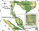
Peninsular Thailand is the most botanically and geographically diverse part of the country (van Steenis Reference van Steenis1950, Woodruff Reference Woodruff2003). In only 16% of the land area of Thailand, the Peninsula includes well over 50% of the vascular plant diversity of the country. The Khao Chong plot was established within Khao Banthad Wildlife Sanctuary, adjacent to Khao Chong Peninsular Botanical Garden, Trang Province, Thailand (7°32′31.67′′N, 99°47′41.22′′E; Figure 1). The plot is ~120 km north of the Kangar–Pattani line, where the climate shifts from aseasonal with no regular annual dry season in the south, to seasonal with a 2- to 3-mo annual dry season in the north. This leads to a shift in forest type from aseasonal mixed dipterocarp forests to seasonal evergreen forests (Ashton Reference Ashton and EO1995, Bunyavejchewin et al. Reference Bunyavejchewin, Baker, Davies, McShea, Davies and Bhumpakphan2011).
Map of Peninsular Thailand with the location of the 24-ha plot at Khao Chong.

The Khao Chong forest is lowland wet seasonal evergreen tropical forest (Bunyavejchewin et al., Reference Bunyavejchewin, Baker, Davies, McShea, Davies and Bhumpakphan2011; or southern seasonal evergreen forest, sensu Ashton Reference Ashton2015), with a 30–35-m-tall canopy and emergent trees reaching 40–45 m (Ogawa et al. Reference Ogawa, Yoda, Kira, Ogino, Shidei, Ratanawongse and Apasutaya1965). Despite a short dry season, the forest is evergreen and resembles lowland mixed dipterocarp forest (MDF) of aseasonal climates further south in total basal area, density of large stems, and relative above-ground biomass (AGB) of dipterocarps (Ashton & Hall Reference Ashton and Hall1992, Davies & Becker Reference Davies and Becker1996, Davies et al. Reference Davies, Nur Supardi, LaFrankie, Ashton, Okuda, Manokaran, Thomas and Ashton2003). The forest differs from MDF in having somewhat lower species richness, fewer individual dipterocarp species, a higher abundance of lianas, a larger fraction of species that are briefly dry-season deciduous, a lower density of small tree stems (Bunyavejchewin et al. Reference Bunyavejchewin, Baker, Davies, McShea, Davies and Bhumpakphan2011) and regular annual reproduction (Kurten et al. Reference Kurten, Bunyavejchewin and Davies2018). Woody climbers are abundant (Ashton Reference Ashton2015, Ogawa et al. Reference Ogawa, Yoda, Kira, Ogino, Shidei, Ratanawongse and Apasutaya1965), and large canopy gaps often result in thickets of climbers. Peak flowering occurs at the end of the dry season in April, and peak fruiting occurs early in the wet season in June–August (Kurten et al. Reference Kurten, Bunyavejchewin and Davies2018). Compared with other tropical seasonal forests, Khao Chong has exceptionally high tree species diversity (Bunyavejchewin et al. Reference Bunyavejchewin, Baker, Davies, McShea, Davies and Bhumpakphan2011, Pyke et al. Reference Pyke, Condit, Aguilar and Lao2001).
The plot sits on steep slopes on the western edge of the Nakhon Si Thammarat range in Peninsular Thailand. The soils are sandy loam, derived from Early Jurassic porphyritic granite of the Khao Kachong Batholith, a linear batholith that forms part of a chain of granites running through Peninsula Thailand, with scattered unweathered boulders both on and under the soil surface (Baillie et al. Reference Baillie, Bunyavejchewin, Kaewfoo, Baker and Hallett2018, Bunyavejchewin et al. Reference Bunyavejchewin, Baker, Davies, McShea, Davies and Bhumpakphan2011, Cobbing Reference Cobbing, Ridd, Barber and Crow2011, Ogawa et al. Reference Ogawa, Yoda, Kira, Ogino, Shidei, Ratanawongse and Apasutaya1965). Overall, the soils are relatively infertile, although spatially heterogeneous within the plot.
Climate
Khao Chong receives an average (± SE) of 2870 ± 115 mm y−1 of rain based on 2000–2015 measurements at the Khao Chong Peninsular Botanical Garden. A short dry season of 1–3 mo (mean = 2.0 mo) with <100 mm of rain occurs from January to March. While Khao Chong is too far south to be directly impacted by typhoon winds, strong tropical storms occasionally make landfall further north in Peninsular Thailand and may result in damaging winds in the Khao Chong area. For example, a particularly destructive tropical storm (Harriet) made landfall in the peninsula not far north of Khao Chong in 1962, and several strong storms were reported in 1966 and 1969 that likely affected Khao Chong (Thai Meteorological Department 2016).
Plot
In 2000, a 24-ha (600 × 400 m) long-term ecological research plot was established in the Khao Chong forest to monitor all woody plants ≥1 cm diameter at breast height (dbh) following methods of the Center for Tropical Forest Science – Forest Global Earth Observatory (Anderson-Teixeira et al. Reference Anderson-Teixeira, Davies, Bennett, Gonzalez-Akre, Muller-Landau and Wright2015, Condit Reference Condit1998, Manokaran et al. Reference Manokaran, LaFrankie, Kochummen, Quah, Klahn, Ashton and Hubbell1990). All free-standing trees ≥1 cm dbh were tagged, mapped to ±10 cm, their dbh measured to ±1 mm, and identified to species. The plot was recensused in 2005 and 2010 following the same protocols, providing information on tree growth, mortality and recruitment.
The 24-ha Khao Chong plot included a total of 119 259 individual trees with 151 945 stems across the three censuses. There were 610 recorded morphospecies, of which 578 morphospecies (118 265 trees; 99.2% of all trees) were single taxa, and 32 morphospecies codes (994 trees; 0.8%) were unresolved, including more than one taxon, or unidentified and may be part of existing morphospecies. Of the 578 distinct morphospecies (hereafter species), 506 (115 578 trees; 96.9%) were named to the species or subspecies level and 72 (2687 trees; 2.3%) remain to be confirmed (e.g. Chionanthus sp. 1 or Palaquium cf. impressionervium). Species were classified as pioneer or non-pioneer trees based on field observations of the species’ propensity to colonize light gaps within the forest, and to occupy open areas along forest edges and roadsides (Davies & Bunyavechewin, pers. obs.). These observations were supported by information derived from regional floristic treatments (including Flora of Thailand, Gardner et al. Reference Gardner, Sidisunthorn and Chayamarit2015, Reference Gardner, Sidisunthorn and Chayamarit2016).
Disturbance history
The plot is in primary or old-growth lowland tropical forest. There is no known history of logging among the large trees, however areas north of the plot were selectively logged in the 1950s and 1960s. In 1981, a landslide associated with extreme rainfall occurred in the south-east corner of the plot, affecting a swathe of forest along the eastern portion of the plot. The soil surface in this area is covered with boulders and exposed mineral soil, and a small seeping spring. The landslide was recorded by local researchers and park authorities (Bunyavejchewin, pers. obs.). Our field observations suggested that another, much older, disturbance affected the lower area in the north of the plot, although no human knowledge of the event exists. The presence of bent and twisted large stems and a stand of large individuals of the early successional species, Alstonia scholaris, suggested a strong wind disturbance may have affected about 3–4 ha near the northern edge of the plot. The date of this disturbance is unknown but we suspect it occurred in or near the 1960s. Analysis of aerial photos from 1972–1983 shows regrowth from a disturbance event in this part of the plot, however we cannot pinpoint the exact timing of the event. In neither disturbance do we know the exact spatial extent of the affected area within the plot. The area impacted was inferred from the distribution of early-successional species. It is likely the disturbances overlap in the north-east corner of the plot.
Soil analysis
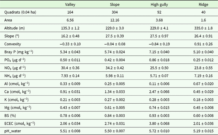
Soil cores were taken from 225 points distributed across the 24-ha plot. One sample was taken at the centre of each 40 × 40-m quadrat (n = 150) and an additional sample was taken 2, 8 or 20 m in a randomly chosen direction from half of the 40 × 40 samples. Soil samples were taken from the upper 10 cm of the soil, which contains the majority of the fine roots and integrates the nutrient cycle. Soil samples were analysed for pH, extractable (plant-available) phosphorus (P), nitrogen (N) mineralization rate, effective cation exchange capacity (ECEC), base saturation (BS), exchangeable cations (Al, Ca, Fe, K, Mg, Mn, Na), and total exchangeable bases (TEB) (Table 1). Exchangeable cations, pH and plant-available P were measured on soils that had been air-dried at ambient laboratory temperature and sieved at 2 mm. Nitrogen mineralization was determined using in-field ion-exchange resins at the same sites as soil collection. The bags contained 5-g of mixed-bed ion-exchange resin (Dowex Marathon Mr-3) enclosed in a 6 × 7.5-cm mesh envelope (polyester monofilament, 220-micron mesh opening) sewed with monofilament thread. Bags were inserted into the upper mineral soil horizon by making a 45° cut with a machete, inserting the bag, and gently pressing the soil surface to enclose the bag in the soil. Bags were retrieved after ~3 wk, rinsed thoroughly in deionized water, and then nutrients were extracted with 75 mL of 0.5 M HCl, with simultaneous determination of NH4, NO3 and PO4 in neutralized extracts by automated colorimetry on a Lachat QuikChem 8500 (Hach Ltd, Loveland, CO). NH4 and NO3 concentrations are a time-integrated measure of nitrogen mineralization during the study period, whereas we interpret PO4 concentrations as reflecting a dynamic equilibrium between the resin and the soil. Soil pH was measured in a 1:2 soil:solution ratio in both water and 10 mM CaCl2 using a glass electrode. Exchangeable cations were measured by extraction in 0.1 M BaCl2 (2 h, 1:30 soil to solution ratio), with detection by inductively coupled plasma optical-emission spectrometry on an Optima 7300 DV (Perkin-Elmer, Shelton, CT, USA) (Hendershot et al. Reference Hendershot, Lalande, Duquette, Carter and Gregorich2008). Plant-available P was extracted in Bray-1 solution, with detection by automated molybdate colorimetry on a Lachat Quikchem 8500 (Hach). Total exchangeable bases (TEB) were calculated as the sum of the charge equivalents of Ca, K, Mg and Na, effective cation exchange capacity (ECEC) was calculated as the sum of Al, Ca, Fe, K, Mg, Mn and Na, and base saturation was calculated as (TEB/ECEC). Soil variables were individually kriged to provide values for each 20 × 20-m quadrat (John et al. Reference John, Dalling, Harms, Yavitt, Stallard, Mirabello, Hubbell, Valencia, Navarrete, Vallejo and Foster2007).
Soil chemical and physical properties (mean ± 1 SE) of four habitats in the 24-ha plot in Khao Chong, Thailand. Altitude, slope and convexity are the mean values per habitat based on 0.04-ha quadrat values. Soil variables are mean values based on kriged estimates at the 0.04-ha quadrat scale: extractable (plant-available) phosphorus (Bray P), resin-bag derived phosphate (PO4), nitrate (NO3) and ammonium (NH4), exchangeable cations aluminium (Al), calcium (Ca), potassium (K) and magnesium (Mg), base saturation (BS), effective cation exchange capacity (ECEC), and soil pH measured in water.

Habitat characterization based on soil chemistry and topography
The plot spans 250 m altitude from 110 to 360 m asl. Three topographic variables for each 20 × 20-m quadrat were derived from the field topographic survey: mean elevation (mean elevation of the four plot corners), slope (the average angle of the quadrat from the horizontal) and convexity (mean elevation of the focal quadrat minus the mean elevation of the eight neighbouring quadrats, with convexity of edge quadrats defined internally as the elevation of the centre point minus the mean elevation of the four corners) using the CTFS R package (http://ctfs.si.edu/Public/CTFSRPackage/).
Topographic variables and soil variables kriged to the quadrat scale were combined and analysed with a range of agglomerative hierarchical clustering techniques to define distinct physico-chemical (edaphic) habitats within the plot. Results based on clustering with Ward’s minimum variance method are presented, but different methods consistently identified similar habitats. Cluster analyses were conducted using JMP version 12.1.0 (SAS Institute).
Species and community composition in relation to habitat variation
Several methods were used to investigate the relationships between species and community composition and edaphic variation in the plot. Torus-translation tests were used to test for individual species habitat associations (Harms et al. Reference Harms, Condit, Hubbell and Foster2001; https://forestgeo.github.io/fgeo/). Mantel and Partial Mantel analyses tested for significant relationships between soil chemistry and topographic, and floristic variation. The floristic similarity matrix of species by quadrat for this analysis was created with Bray–Curtis similarity values. Topography (slope, elevation and convexity) and soil chemistry (soil chemical traits described above) matrices were based on Euclidean distance. Analyses were conducted using Vegan R package version 2.5-3 (https://CRAN.R-project.org/package=vegan).
To investigate the relationships between floristic composition and edaphic variation among quadrats, we first conducted a cluster analysis of the floristic composition to identify groups of similar floristic areas within the plot. We then used discriminant analysis to assess whether the environmental variables supported the groupings derived from the floristic analysis and to determine which environmental variables were most strongly associated with the floristic groups (Legendre & Legendre Reference Legendre and Legendre1998). Cluster analysis of floristic composition used Ward’s minimum variance method.
Stand structure and demographic analyses
Above-ground biomass (AGB) for individual trees was estimated using the moist forest regression model without tree height (Chave et al. Reference Chave, Andalo, Brown, Cairns, Chambers, Eamus, Folster, Fromard, Higuchi, Kira, Lescure, Nelson, Ogawa, Puig, Riera and Yamakura2005). Species’ wood density values were derived from Chave et al. (Reference Chave, Coomes, Jansen, Lewis, Swenson and Zanne2009). For 207 species, Chave et al. (Reference Chave, Coomes, Jansen, Lewis, Swenson and Zanne2009) included a species-level value. In the absence of a species-level value, we used the genus-level mean (326 species), the family-level mean (72 species), or the plot-wide mean (5 species). We quantified AGB fluxes due to growth, recruitment and mortality for the whole plot and for each habitat separately using the 2000 and 2010 censuses. Confidence intervals were estimated from 1000 bootstraps using individual quadrats.
Instantaneous mortality was calculated as (log N1−log S2)/T and instantaneous recruitment was calculated as (log N2−log S2)/T, where N1 and N2 are the number of individuals alive in census 1 and census 2 respectively, S2 is the number of individuals surviving to census 2, and T is the interval between censuses in years (Condit et al. Reference Condit, Ashton, Manokaran, LaFrankie, Hubbell and Foster1999). Annual growth was the diameter increment (dbh2−dbh1)/T, for the main stem of each individual tree, discarding outliers following Condit et al. (Reference Condit, Aguilar, Hernandez, Perez, Lao, Angehr, Hubbell and Foster2004). Analyses were conducted using RStudio 1.1.456 (https://CRAN.R-project.org).
Results
Forest composition
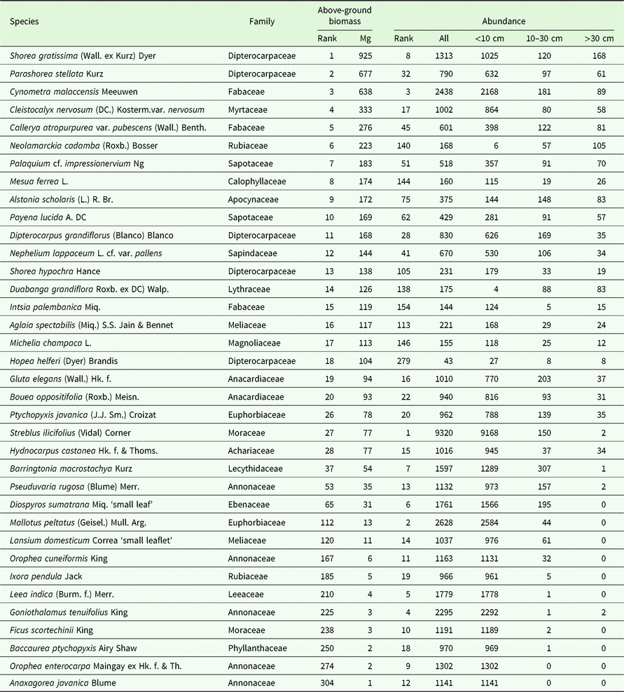
Total tree species diversity in 2000 was 575 species, with a Fisher’s alpha of 80.6. The subcanopy tree, Streblus ilicifolius, was the most common species with 8.8% of all individuals (Table 2). Shorea gratissima, Parashorea stellata and Cynometra malaccensis had the most biomass, together accounting for 24.4% of overall biomass in 2000 (Table 2). Trees in the Annonaceae and Moraceae had the most stems, and the Dipterocarpaceae and Fabaceae had most above-ground biomass (Appendix 1). The commonest genera were Streblus, Diospyros and Ficus. Shorea, Parashorea and Cynometra had the most biomass (Appendix 2). Fifty-seven species of pioneer trees, comprising 5268 individuals (5.2%), were recorded in the plot in 2000.
Species composition of the 24-ha plot in Khao Chong, Thailand. List includes the top 20 species in AGB contribution and individual abundance in 2000. AGB in Mg for the whole plot. Abundances for all stems and in dbh size classes in cm. For Diospyros sumatrana and Lansium domesticum two subspecific morphospecies were recognized within the plot. Since these morphotypes are not named, we refer to them by an easily recognized morphological feature.

Habitat variation
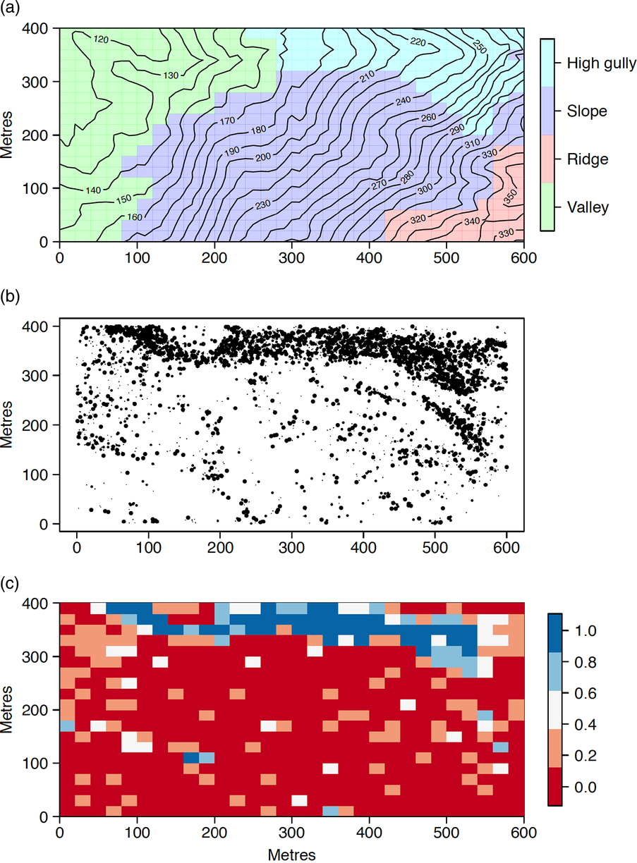
Cluster analysis of soil chemistry and topographic variables identified four main edaphic habitats within the 24-ha plot: valley, slope, high gully and ridge (Figure 2). The valley, in the lowest part of the plot, is on flatter terrain with shallow concave slopes, moderate NO3 mineralization, relatively low base status and includes a semi-permanent stream (Table 1). The slope on steep ground had relatively high N concentrations and otherwise intermediate fertility. The high gully on very steep concave surfaces had the highest pH, available P and base cation concentrations, but lower N concentrations. The ridge at the highest point in the plot on convex, steep topography is the most acidic and infertile habitat (Table 1).
Maps of topography and edaphic habitats, and pioneer trees in the 24-ha plot in Khao Chong, Thailand. Habitats, defined as: valley (green), slope (purple), high gully (light blue) and ridge (red) (a). Distribution of pioneer trees with point size scaled to dbh (b). Relative contribution of pioneer species to AGB per quadrat (0.04 ha) (c). For all maps the x-axis is from north (left) to south (right).

The two disturbance events, defined by the presence of pioneer trees, were concentrated in the valley and high gully habitats (Figure 2). The 1981 landslide extended from the high gully habitat down to the valley habitat in a long strip along the east of the plot. The older putative 1960s wind disturbance affected an area in the north and north-east section of the valley habitat (Figure 2).
Habitat effects on species composition
Individual species were strongly spatially aggregated within the plot. For species with more than 50 individuals in 2000, 208 of 268 species (78%) had spatial distributions significantly aggregated or repelled from at least one of the four habitats. Consequently, each of the four habitats had characteristic common species (Appendix 3). Many of the species with strong affinities for the high gully are early successional, including species of Ficus and Macaranga. The slope habitat was dominated by shade-tolerant mid-canopy species, with high abundances of Streblus ilicifolius.
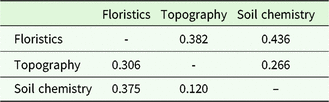
At the 0.04-ha scale, there were strong relationships among floristic composition, soil chemistry and topography within the plot (Table 3). Despite the large variation in topography (Figure 2), floristic composition was more strongly associated with soil chemistry than with topography (P ≤ 0.001). The Partial Mantel statistic was greater for floristics versus chemistry (holding topography constant) than floristics versus topography (holding chemistry constant).
Summary of Mantel tests for relationships among floristic composition, topography and soil chemistry in the 24-ha plot in Khao Chong, Thailand. Values above the diagonal are pairwise standardized Mantel statistics. Values below the diagonal are Partial Mantel statistics. All analyses were significant at P ≤ 0.001.

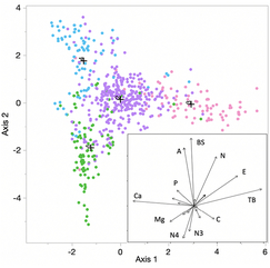
Discriminant analysis of soil chemistry and topography supported the cluster analysis of species composition across the plot (Figure 3). Total exchangeable bases (TEB) and mean elevation were positively correlated, and Ca negatively correlated with the first axis of the canonical ordination. Al, base saturation (BS) and total N were strongly positively correlated with the second axis. Misclassifications in the discriminant analysis (18% of 600 quadrats) mostly involved quadrats on the margins of the habitats, particularly on the margins of the slope habitat. The ridge, high gully and valley habitats had very distinct species compositions. The slope habitat in the central part of the plot was intermediate between the other habitats in both species composition and soil chemistry (Table 1).
Canonical ordination plot from discriminant analysis of soil chemistry and topography constrained by four floristic subcommunities defined by cluster analysis. Points in the canonical plot are edaphic data for 600 0.04-ha subquadrats (Figure 2). Colours indicate floristic subcommunities, valley (green), slope (purple), high gully (light blue) and ridge (red), based on Ward’s minimum variance cluster analysis of species composition for the 2000 census. Crosses indicate multivariate mean values for the four subcommunities. The first two axes explained 78% of the variance. Per cent misclassification = 18%. Inset shows contributions of the biophysical variables to the first two canonical axes, including Ca, calcium, P, phosphate, Mg, magnesium, N4, ammonium, N3, nitrate, C, effective cation exchange capacity, TB, total bases, E, mean elevation, N, total nitrogen, BS, base status, and A, aluminium.

Habitat and pioneer trees
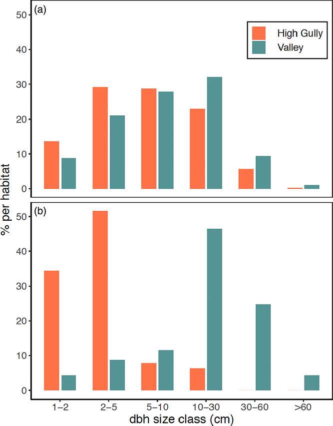
The distribution of the pioneer trees was strongly spatially aggregated (Figure 2) and their abundance and structure varied significantly among habitats. The high gully (22% of stems) and the valley (7%) had much higher numbers of pioneer trees than the other two habitats (range 1–2%). The valley and high gully habitats differed significantly in the size distribution of the pioneers (KS, P < 0.01; Figure 4). The valley had fewer small and more large pioneer trees. This was particularly evident for the large-statured pioneer, Alstonia scholaris where 70% of the stems in the valley were ≥30 cm dbh, and only 11% of the stems were ≥30 cm in the high gully (Figure 4).
Size distribution of pioneer trees in disturbed habitats (valley and high gully) in the 24-ha plot in Khao Chong, Thailand. All trees of 57 pioneer species (a). Trees of Alstonia scholaris (b).

Forest structure and dynamics
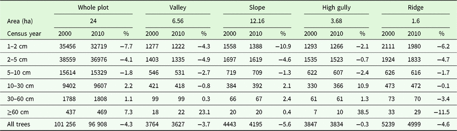
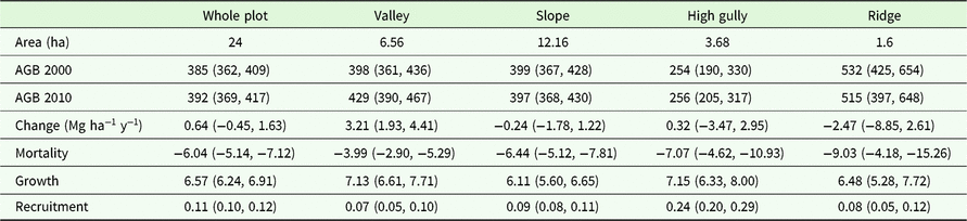
In 2000, the 24-ha plot included 101 256 individual trees ≥1 cm dbh (mean: 4218 ha−1) and 11 574 trees ≥10 cm dbh (mean: 482 ha−1). Tree number declined to 96 908 by 2010 (Table 4). Over 10 y, there was a decline in the number of trees ≤10 cm dbh, and an increase in the number of trees ≥10 cm dbh (KS test, P < 0.01). Mean plot AGB was 385 Mg ha−1 in 2000 (Table 5). The increase in the number of larger stems meant that AGB gain due to growth exceeded AGB loss due to mortality, leading to a small but not significant increase in AGB of 0.64 Mg ha−1 y−1 to 392 Mg ha−1 from 2000 to 2010 for the plot as a whole (Table 5).
Stem size distributions for trees in the 24-ha plot and for four edaphic habitats for the 2000 and 2010 censuses in the 24-ha plot in Khao Chong, Thailand. % indicates the per cent change over 10 y for each size class.

Total above-ground biomass (AGB, Mg ha−1), AGB dynamics, and AGB change partitioning among mortality, growth and recruitment in the 24-ha plot in Khao Chong, Thailand, and four edaphic habitats in 2000 and 2010. AGB confidence intervals estimated at the 0.04-ha scale using bootstrapping.

Habitat effects on forest structure and dynamics
Stand structure and dynamics varied significantly within the plot. The high gully was the most structurally distinct habitat with just 254 Mg AGB ha−1 in 2000. The ridge had over 530 Mg AGB ha−1, and the slope and valley habitats were intermediate with ~398 Mg AGB ha−1 (Table 4). Tree size distributions also differed significantly among habitats (KS test, P <0.001). The ridge had more very large trees (≥60 cm dbh), the valley had fewer small stems (<5 cm dbh), and the high gully had many fewer large stems (>30 cm dbh, Table 4).
AGB increased in the valley and high gully, and decreased in the slope and ridge, but only in the valley did AGB change significantly (+3.21 Mg ha−1 y−1; Table 5). The number of stems ≥1 cm dbh declined in all habitats (Table 4). The number of large stems increased in the valley and high gully. The significant AGB increase in the valley was the result of high AGB gain from growth coupled with much lower AGB loss to mortality compared with the other habitats (Table 5).
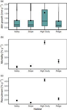
At the individual level, the high gully was by far the most dynamic habitat with about double the average dbh growth, mortality and recruitment rates as the other habitats (Figure 5). The ridge had the lowest growth rates, but relatively high mortality and recruitment rates. The valley and slope had relatively low individual growth, mortality and recruitment rates.
Demographic rates in four edaphic habitats in the 24-ha plot in Khao Chong, Thailand. Growth (a), mortality (b) and recruitment (c) rates for the entire census period from 2000 to 2010. Points in growth boxplots indicate mean annual growth rates. For mortality and recruitment 95% confidence intervals were estimated from 1000 bootstraps using individual quadrats in each habitat.

Discussion
Disturbance and habitat variation in Khao Chong
The location for the Khao Chong plot was selected to represent primary forest. However, we found evidence for two major natural disturbances within the 24-ha plot that had dramatic effects on soil conditions, floristic composition, stand structure and forest dynamics. A landslide associated with extreme rainfall in 1981 led to a multi-hectare canopy opening, the downhill redistribution of soil and rocks, and the exposure of mineral subsoil (high gully). This disturbance was easily recognized by the elevated soil nutrient conditions, relatively low AGB, and abundance of pioneer trees. An earlier disturbance in the lower section of the plot occurred some 50–70 y ago and while the cause of that disturbance remains unknown, we suspect it may have been the result of a rare local windstorm that knocked down a swathe of forest within and outside the plot (valley). This disturbance was evident through analysis of stand structure and species composition. Such large windstorms are rare this close to the equator in Asia.
Despite uniform geology across the plot, edaphic conditions at the local scale were heterogeneous due to both the recent disturbance and the considerable topographic relief. The 1981 landslide had a strong effect on soil nutrient concentrations. Local scale tree-falls and landslides may result in short-term increases in soil fertility, followed by declines in nutrient status as the forest regrows (Roberts & Gilliam Reference Roberts and Gilliam1995, Shiels & Walker Reference Shiels and Walker2013, Walker et al. Reference Walker, Shiels, Bellingham, Sparrow, Fetcher, Landau, Lodge and Kitzberger2013). Comparing our recent and older disturbed habitats, and assuming soil fertility is fairly uniform away from the ridge in the plot, this pattern appears to hold at Khao Chong. We anticipate that soil nutrient availability in the high gully habitat will decline as the forest regenerates.
Topography was also an important driver of spatial variation in soil fertility within the plot. The ridge habitat had the lowest nutrient status among the four habitats. Topographic effects on soil nutrient status have been widely observed in tropical forests (Chadwick & Asner Reference Chadwick and Asner2016, Weintraub et al. Reference Weintraub, Taylor, Porder, Cleveland, Asner and Townsend2015). In most ridge-valley catena systems, ridge habitats have reduced fertility compared with adjacent valleys through movement of fine material and nutrients downslope. In addition, strongly convex slopes and sandy soils likely lead to increased drainage and periodic water stress in the ridge habitat (Russo et al. Reference Russo, Cannon, Elowsky, Tan and Davies2010).
Disturbance and habitat effects on species composition
The combined effects of disturbance history and topography led to strongly aggregated species distributions at Khao Chong. More than 75% of species had spatial distributions significantly associated with edaphic conditions. While high levels of species’ habitat association are widespread in tropical forests (Allie et al. Reference Allie, Pelissier, Engel, Petronelli, Freycon, Deblauwe, Soucemarianadin, Weigel and Baraloto2015, Harms et al. Reference Harms, Condit, Hubbell and Foster2001, John et al. Reference John, Dalling, Harms, Yavitt, Stallard, Mirabello, Hubbell, Valencia, Navarrete, Vallejo and Foster2007), Khao Chong is at the very high end of habitat specialization recorded (Davies et al. Reference Davies, Tan, LaFrankie, Potts, Roubik, Sakai and Karim2005, Gunatilleke et al. Reference Gunatilleke, Gunatilleke, Esufali, Harms, Ashton, Burslem and Ashton2006). All four edaphic habitats had a unique set of specialists, resulting in strong compositional turnover across the plot. Strong species compositional turnover at a local scale has been associated with gradients in topography (Baldeck et al. Reference Baldeck, Harms, Yavitt, John, Turner, Valencia, Navarrete, Davies, Chuyong, Kenfack, Thomas, Madawala, Gunatilleke, Gunatilleke, Bunyavejchewin, Kiratiprayoon, Yaacob, Supardi and Dalling2013, Valencia et al. Reference Valencia, Foster, Villa, Condit, Svenning, Hernández, Romoleroux, Losos, Magård and Balslev2004), soil nutrients (John et al. Reference John, Dalling, Harms, Yavitt, Stallard, Mirabello, Hubbell, Valencia, Navarrete, Vallejo and Foster2007, Tuomisto et al. Reference Tuomisto, Ruokolainen and Yli-Halla2003) and hydrological conditions (Schietti et al. Reference Schietti, Emilio, Rennó, Drucker, Costa, Nogueira, Baccaro, Figueiredo, Castilho, Kinupp, Guillaumet, Garcia, Lima and Magnusson2013). We showed that both soil chemistry and topography had significant and independent effects on turnover across the plot, with soil chemistry more strongly affecting species turnover than topography (see also Davies et al. Reference Davies, Tan, LaFrankie, Potts, Roubik, Sakai and Karim2005). A more mechanistic understanding of how these patterns are established and maintained will require experimental studies of species’ responses to resource gradients.
While soils and topography explained a large fraction of the variation in species composition at Khao Chong, significant spatial variation in floristic composition remained unexplained (Baldeck et al. Reference Baldeck, Harms, Yavitt, John, Turner, Valencia, Navarrete, Davies, Chuyong, Kenfack, Thomas, Madawala, Gunatilleke, Gunatilleke, Bunyavejchewin, Kiratiprayoon, Yaacob, Supardi and Dalling2013). The discriminant analyses revealed 18% mismatch between the floristic classification and that derived from soil chemistry and topography. The four habitats were defined based solely on soils and topography, and did not include disturbance history since we did not have precise knowledge of their areas of impact. Disturbance history appears to have had additional independent effects on species’ distributions at Khao Chong. The disturbances did not map directly onto the edaphic habitats. The older disturbance affected part of the valley, and the landslide affected parts of the valley and high gully. Many of the mismatched quadrats were on the margins of other habitats but were dominated by pioneer species. In these cases, it seems likely that canopy light availability overrode soils and topography in driving species’ spatial distributions. It is also possible that the plot coverage for the soil analysis lacked resolution in some areas. For example, the soil map does not detect slope habitats along the south-eastern edge of the plot.
Disturbance and habitat effects on stand structure and dynamics
Stand structure varied among habitats as predicted from local edaphic conditions and disturbance history. The ridge was structurally unique with very high AGB, stem densities and abundance of smaller stems. High biomass and big-tree density are common on well-drained, lower fertility ridges in dipterocarp forests and more generally in tropical forests (Lee et al. Reference Lee, Davies, LaFrankie, Tan, Itoh, Yamakura, Ohkubo and Ashton2002, Valencia et al. Reference Valencia, Condit, Muller-Landau, Hernandez and Navarrete2009). High stem densities in small size classes are also a common feature of ridges (Lee et al. Reference Lee, Davies, LaFrankie, Tan, Itoh, Yamakura, Ohkubo and Ashton2002), possibly linked to the higher understorey light levels (Russo et al. Reference Russo, Cannon, Elowsky, Tan and Davies2010). The high gully had many small stems, few large stems, low standing AGB and abundant fast-growing pioneers, reflecting the impacts of the recent landslide. The valley had a stand of large individuals of the successional species, Alstonia scholaris, a remnant from a large disturbance. This species was associated with a dense patch of medium to large individuals of Shorea gratissima, an emergent dipterocarp. We suspect that larger S. gratissima individuals were released following the earlier disturbance, and with Alstonia are continuing to grow fast, resulting in positive AGB accumulation in the valley.
Overall, the Khao Chong forest showed a non-significant trend of increasing AGB of 0.64 Mg ha−1 y−1 over 10 y. Increasing AGB trends have been reported from forests in the Amazon (Brienen et al. Reference Brienen, Phillips, Feldpausch, Gloor, Baker and Lloyd2015, Phillips et al. Reference Phillips, Malhi, Higuchi, Laurance, Nunez, Vasquez, Laurance, Ferreira, Stern, Brown and Grace1998), Africa (Lewis et al. Reference Lewis, Lopez-Gonzalez, Sonke, Affum-Baffoe, Baker and Ojo2009) and Borneo (Qie et al. Reference Qie, Lewis, Sullivan, Lopez-Gonzalez, Pickavance and Sunderland2017). The magnitude of the change at Khao Chong is similar to levels reported in these studies. Given that the Khao Chong plot is in old-growth forest, and without knowledge of the local natural disturbance history, it is tempting to infer that the Khao Chong forest is accumulating AGB for reasons of increased resource availability (e.g. increased atmospheric CO2). However, the AGB increase was entirely due to the two habitats that were recovering after natural disturbance. The slope and ridge habitats, covering over 50% of the plot area, had no significant change in AGB.
As the large Alstonia trees in the valley begin to senesce, we expect total AGB to decline over the coming decades. The remaining large trees of S. gratissima will continue to grow quickly as light conditions improve with reduced competition, but their AGB uptake through growth is unlikely to balance the AGB lost through mortality of the big pioneers. In the absence of further perturbation, we predict a reversal of the AGB balance over the coming decades. Forest composition and stand structure provide detailed insights into likely drivers of AGB change in forests. In many field studies of AGB change in tropical forests, there is little or no assessment of underlying forest compositional or stand structural variation with which to interpret AGB changes (but see Chave et al. Reference Chave, Condit, Muller-Landau, Thomas, Ashton and Bunyavejchewin2008, Feeley et al. Reference Feeley, Davies, Ashton, Bunyavejchewin, Nur Supardi, Kassim, Tan and Chave2007). While it is unsurprising that the disturbed habitats increased AGB over the course of our study (Poorter et al. Reference Poorter, Bongers, Aid, Almeyda Zambran, Balvanera and Becknell2016), further work is required to determine whether external anthropogenic drivers, such as elevated CO2 or temperature, are shifting the rate of recovery in the disturbed sections of the Khao Chong forest.
Acknowledgements
The Khao Chong Forest Dynamics Plot involves collaboration between the Royal Forest Department, Thailand; the Department of National Parks, Wildlife and Plant Conservation; Kasetsart University Faculty of Forestry; and the Center for Tropical Forest Science – Forest Global Earth Observatory of the Smithsonian Tropical Research Institute. Funding for this work has come from The Conservation, Food and Health Foundation; the Asia program of the Arnold Arboretum at Harvard University; CTFS–ForestGEO; and NSF awards DEB-1046113 and DEB-1545761 to S.J.D. We thank Nantachai Pongpattananurak for help with locating aerial photos of Khao Chong; Daniel Zuleta for analytical advice; Jim Dalling for advice on the soil sampling design; Dayana Agudo and Aleksandra Bielnicka for laboratory support; and Preecha Puttarak and the entire Khao Chong field team for their long-term commitment to the plot. We also thank the staff of the Khao Chong Peninsular Botanical Garden for their support throughout the project. Peter Ashton, Patrick Baker, Gabriel Arellano and Egbert Leigh provided comments on the manuscript.
Financial support
Center for Tropical Forest Science–Forest Global Earth Observatory, Smithsonian Institution; The Conservation, Food and Health Foundation; Asia program of the Arnold Arboretum at Harvard University; NSF awards DEB-1046113 and DEB-1545761.
Appendix 1
Structure and diversity of the 20 most important tree families in the 24-ha plot in Khao Chong, Thailand.

Appendix 2
Structure and diversity of the 20 most important tree genera in the 24-ha plot in Khao Chong, Thailand. Three additional genera have five species in the plot: Mallotus, Nephelium and Xanthophyllum.

Appendix 3
Common species distribution patterns with respect to edaphic habitats in the 24-ha plot in Khao Chong, Thailand. Habitat specialists arranged in rows, first row ridge (a), (b), second valley (c), (d), third slope (e), (f) and fourth high-gully (g), (h) specialists. For Diospyros sumatrana ‘small’ is the small-leaved, sub-specific morphospecies recognized within the plot.