2.1 Governing equations

Figure 1.

Sketch of the computational model for shear-driven shallow-water turbulence with LCs.

Figure 1 shows the computational domain and coordinates used in the present simulations. As shown, $x$ , $y$ and $z$ represent the streamwise, vertical and spanwise directions, respectively. The water depth is $H$ . Wall-resolved LES based on the C–L equations is performed to study the neutrally stratified shallow-water Langmuir turbulence. Following McWilliams et al. (Reference McWilliams, Sullivan and Moeng1997), a low-pass spatial filter is applied to obtain the wave-phase-averaged motions. The C–L equations read

(2.1) $$\begin{eqnarray}\displaystyle & \displaystyle \unicode[STIX]{x1D735}\boldsymbol{\cdot }\overline{\boldsymbol{u}}=0, & \displaystyle\end{eqnarray}$$

(2.2) $$\begin{eqnarray}\displaystyle & \displaystyle \frac{\unicode[STIX]{x2202}\overline{\boldsymbol{u}}}{\unicode[STIX]{x2202}t}+\overline{\boldsymbol{u}}\boldsymbol{\cdot }\unicode[STIX]{x1D735}\overline{\boldsymbol{u}}=-\unicode[STIX]{x1D735}\overline{\unicode[STIX]{x1D6F1}}+\unicode[STIX]{x1D708}\unicode[STIX]{x1D6FB}^{2}\overline{\boldsymbol{u}}+\unicode[STIX]{x1D735}\boldsymbol{\cdot }\unicode[STIX]{x1D749}^{sgs}+\boldsymbol{u}_{s}\times \overline{\unicode[STIX]{x1D74E}}. & \displaystyle\end{eqnarray}$$

Here, $\overline{\boldsymbol{u}}=(\overline{u},\overline{v},\overline{w})$ is the resolved velocity with $\overline{u}$ , $\overline{v}$ and $\overline{w}$ denoting the velocity in the $x$ -, $y$ - and $z$ -directions, respectively. The overline represents the implicit grid-level filter. The effective pressure $\overline{\unicode[STIX]{x1D6F1}}=\overline{p}/\unicode[STIX]{x1D70C}+\overline{\unicode[STIX]{x1D6E4}}$ includes the resolved pressure $\overline{p}/\unicode[STIX]{x1D70C}$ and the additional term (McWilliams et al. Reference McWilliams, Sullivan and Moeng1997)

(2.3) $$\begin{eqnarray}\overline{\unicode[STIX]{x1D6E4}}={\textstyle \frac{1}{2}}\boldsymbol{u}_{s}\boldsymbol{\cdot }\boldsymbol{u}_{s}+\boldsymbol{u}_{s}\boldsymbol{\cdot }\overline{\boldsymbol{u}}.\end{eqnarray}$$

In (2.2) and (2.3), $\boldsymbol{u}_{s}$ is the Stokes drift velocity induced by water waves. According to Longuet-Higgins (Reference Longuet-Higgins1953) and Phillips (Reference Phillips1967), $\boldsymbol{u}_{s}$ induced by shallow-water potential waves is given as

(2.4) $$\begin{eqnarray}\boldsymbol{u}_{s}(y)=u_{s}^{\ast }\left(\frac{\cosh (2ky)}{2\sinh ^{2}(2kh)},0,0\right)=\frac{u_{\unicode[STIX]{x1D70F}}}{La_{t}^{2}}\left(\frac{\cosh (2ky)}{2\sinh ^{2}(2kh)},0,0\right).\end{eqnarray}$$

Here, $u_{s}^{\ast }=\unicode[STIX]{x1D70E}ka^{2}$ is the characteristic value of $u_{s}$  (Tejada-Martínez & Grosch Reference Tejada-Martínez and Grosch2007), with $\unicode[STIX]{x1D70E}$ , $k$ and $a$ being the frequency, wavenumber and wave amplitude, respectively. In (2.2), $\unicode[STIX]{x1D708}$ is the kinematic viscosity, and the subgrid-scale (SGS) stress tensor $\unicode[STIX]{x1D749}^{sgs}$ is included due to the use of the low-pass spatial filter. The last term on the right-hand side of (2.2) is the C–L vortex force, with $\overline{\unicode[STIX]{x1D74E}}=\unicode[STIX]{x1D735}\times \overline{\boldsymbol{u}}$ being the vorticity. The value of $La_{t}^{2}$ characterizes the relative magnitude of the wind-shear forcing with respect to wave forcing. According to the definitions of the C–L vortex force (2.2) and Stokes drift (2.4), the increase of either $La_{t}$ or $kh$ leads to the magnitude decrease of the C–L vortex force. Particularly, as the value of $La_{t}$ approaches infinity, the flow reduces to a shear-driven turbulence without LCs.

In the C–L equations derived by Craik & Leibovich (Reference Craik and Leibovich1976) and Leibovich (Reference Leibovich1977), the Stokes drift $u_{s}$ is obtained using the leading-order solution of potential waves with respect to the wave steepness $\unicode[STIX]{x1D716}$ . Near the wave surface and water bottom, the magnitude of Stokes drift in the context of viscous flow is different from that obtained from the potential theory due to the viscous boundary condition. For example, at the water bottom, the Stokes drift $u_{s}$ is zero due to the no-slip boundary condition, but the value given by (2.4) is non-zero. Nevertheless, the magnitude of the latter is very small. Among all the cases studied in this paper, the maximal value of $u_{s}$ is $2.26u_{\unicode[STIX]{x1D70F}}$ . Near the water surface, the viscous effect can also influence the Stokes drift. However, the influence of the viscous effect on the Stokes drift is confined in a thin layer. Longuet-Higgins (Reference Longuet-Higgins1953) showed that the leading-order approximation of shallow-water waves satisfies the potential solution in most of the water column, and only deviates from the potential solution in a thin viscous layer with a thickness comparable to that of the Stokes layer. The thickness of the Stokes layer $\unicode[STIX]{x1D6FF}_{s}$ is $\sqrt{2\unicode[STIX]{x1D708}/\unicode[STIX]{x1D70E}}$ , which is small for water waves. For example, in the case of finite-depth waves, if $\unicode[STIX]{x1D70E}=2\unicode[STIX]{x03C0}~\text{rad}~\text{s}^{-1}$ , the thickness of its Stokes layer is only $0.56$  mm (Longuet-Higgins Reference Longuet-Higgins1953). The thickness of the Stokes layer can also be estimated from other studies of turbulent boundary layer subjected to an oscillatory pressure gradient. Based on the results of Ramaprian & Tu (Reference Ramaprian and Tu1983), Scotti & Piomelli (Reference Scotti and Piomelli2001) and Manna, Vacca & Verzicco (Reference Manna, Vacca and Verzicco2012), we can estimate that $\unicode[STIX]{x1D6FF}_{s}$ is smaller than five wall units under the wave condition that Langmuir circulations are observed in the field by Gargett & Wells (Reference Gargett and Wells2007). This above discussions indicate that the viscous effects are confined in the viscous sublayer. According to the original theory of Craik & Leibovich (Reference Craik and Leibovich1976), the viscous effects may lead to a correction to the C–L equation. However, the correction is only subtle and is in a thin layer near the wave surface and water bottom. In Langmuir turbulence, due to the wind shear, the viscous effects near the wave surface and water bottom are much less important than the wind-induced shear. As a result of the above factors, it is believed that the viscous effects at the boundaries only have higher-order influence on the dynamics of the Langmuir turbulence. It was shown in previous LES studies of shallow-water Langmuir turbulence that the LES results based on the C–L equations with $u_{s}$ given by (2.4) (Tejada-Martínez & Grosch Reference Tejada-Martínez and Grosch2007) agree well with the field measurement data (Gargett & Wells Reference Gargett and Wells2007). At last, we remark that when more computer power becomes available, one might conduct wave-phase-resolved simulations with full viscous boundary conditions to quantify the viscous effects at the boundaries, which requires a simulation framework different from the present one based on the C–L equations and is beyond the scope of this work.

The surface boundary for the wave-phase-averaged motions described in the C–L equations is a rigid lid, which is obtained by keeping the leading-order term in the expansion of the boundary condition with respect to the wave steepness (Craik & Leibovich Reference Craik and Leibovich1976; Leibovich Reference Leibovich1977). According to Kemp & Simons (Reference Kemp and Simons1982) and McWilliams, Restrepo & Lane (Reference McWilliams, Restrepo and Lane2004), the difference in wave amplitude induced by wave–current interactions is a higher-order effect with respect to the wave steepness, which is omitted in the C–L theory. Therefore, it is believed that the C–L equation with a rigid-lid boundary condition at wave surface can still be used under the influence of wave–current interaction. In fact, the rigid-lid surface boundary condition has been widely used in LES of Langmuir turbulence (Skyllingstad & Denbo Reference Skyllingstad and Denbo1995; McWilliams et al. Reference McWilliams, Sullivan and Moeng1997; Tejada-Martínez & Grosch Reference Tejada-Martínez and Grosch2007). The flow is driven by a constant wind-shear stress $\unicode[STIX]{x1D70F}_{w}=\unicode[STIX]{x1D70C}u_{\unicode[STIX]{x1D70F}}^{2}$ at the water surface $y=2h$ , with $\unicode[STIX]{x1D70C}$ being the density of water. The no-slip boundary condition is applied at the bottom $y=0$ . Periodic boundary conditions are imposed in the $x$ - and $z$ -directions.

Table 1.

Key parameters of simulation cases.

2.2 Computational parameters

Table 1 summarizes the key parameters of the present simulations. In the table, $L_{x}$ and $L_{z}$ denote the computation domain size in the $x$ - and $z$ -directions, respectively; $N_{x}$ , $N_{y}$ and $N_{z}$ are the number of the grid points in the $x$ -, $y$ - and $z$ -directions, respectively, with $\unicode[STIX]{x0394}x^{+}$ , $\unicode[STIX]{x0394}y_{min}^{+}$ and $\unicode[STIX]{x0394}z^{+}$ being the grid resolution in the corresponding directions. The superscript ‘ $+$ ’ denotes flow quantities normalized using the viscous length scale $\unicode[STIX]{x1D708}/u_{\unicode[STIX]{x1D70F}}$ and surface friction velocity $u_{\unicode[STIX]{x1D70F}}$ . Note that due to the use of a conservative finite difference scheme for the discretization in the $y$ -direction (Kim & Moin Reference Kim and Moin1985), the shear stress $\unicode[STIX]{x1D70F}_{w}$ prescribed at the top is balanced by the time-averaged shear stress at the bottom when the flow is fully developed to a statistically stationary state. Correspondingly, the value of $u_{\unicode[STIX]{x1D70F}}$ at the water bottom obtained from the simulation is also identical to that at the water surface. As a result, the values of $\unicode[STIX]{x0394}x^{+}$ , $\unicode[STIX]{x0394}y_{min}^{+}$ and $\unicode[STIX]{x0394}z^{+}$ are all constants in different cases with the same $Re_{\unicode[STIX]{x1D70F}}$ . The details of the numerical scheme are given in § 2.3.

Simulation cases 1–3 are conducted to study the effect of the Reynolds number $Re_{\unicode[STIX]{x1D70F}}=u_{\unicode[STIX]{x1D70F}}h/\unicode[STIX]{x1D708}$ . The value of $Re_{\unicode[STIX]{x1D70F}}$ is $1000$ , $700$ and $395$ in cases 1, 2 and 3, respectively. The dimensionless parameters $La_{t}=0.7$ and $kh=0.5$ are chosen to match the typical field condition in the observation of Gargett & Wells (Reference Gargett and Wells2007). Cases 3S and 3L are performed to examine the influence of the computational domain size on the simulation results. The values of $Re_{\unicode[STIX]{x1D70F}}$ , $La_{t}$ and $kh$ in cases 3S and 3L are the same as those in case 3. The computational domain sizes of cases 3S and 3L are respectively one-half and four times that of case 3 in both the $x$ - and $z$ -directions. It is shown in § 2.4 that the computation domain size of case  $3$ , $L_{x}\times L_{z}=8\unicode[STIX]{x03C0}h\times 16\unicode[STIX]{x03C0}h/3$ , is sufficiently large to obtain accurate simulation results. As a result, the computational domain size of the other cases is set to that of case 3. Cases 1 and 4–6 are performed to investigate the effect of $kh$ . In these cases, the value of $kh$ varies from $0.5$ to $2.0$ with the corresponding wavelength-to-depth ratio $\unicode[STIX]{x1D706}/H$ varying from $2\unicode[STIX]{x03C0}$ to $\unicode[STIX]{x03C0}/2$ , while $Re_{\unicode[STIX]{x1D70F}}$ and $La_{t}$ are fixed at $1000$ and $0.7$ , respectively. The effect of $La_{t}$ is studied through cases 1, 7 and 8. The value of $La_{t}$ is $0.4$ , $0.7$ and $0.9$ in cases 7, 1 and 8, respectively. Case 9 is the pure shear-driven turbulence case, which is used as a reference case to reveal the influence of LCs on turbulence statistics.

The grid is evenly distributed in the $x$ - and $z$ -directions. In the $y$ -direction, the grid lines are located at $y_{j}/h=b^{-1}\tanh [(-1+2j/N_{y})\tanh ^{-1}(b)]+1$ for $j=0,1,\ldots ,N_{y}$ with $b=0.973$ , such that the grid is clustered near the water surface and water bottom. As shown in table 1, the minimum vertical grid resolution $\unicode[STIX]{x0394}y_{min}^{+}$ near the top and bottom is smaller than $1.0$ , satisfying the grid resolution of wall-resolved LES. The grid resolution in the $x$ - and $z$ -directions also satisfies the standard of wall-resolved LES, i.e. $\unicode[STIX]{x0394}x^{+}\simeq 50$ and $\unicode[STIX]{x0394}z^{+}\simeq 30$  (Chapman Reference Chapman1979; Choi & Moin Reference Choi and Moin2012). We have re-run case 1 by doubling the number of grid points in the $x$ - and $z$ -directions to examine the effect of grid resolution on the simulation results. It is found that the mean velocity and Reynolds stresses change by less than $2\,\%$ and $4\,\%$ , respectively.

2.3 Numerical method

In our simulations, the fractional-step projection method (Kim & Moin Reference Kim and Moin1985) is employed to solve (2.1) and (2.2). The second-order explicit Adams–Bashforth scheme and second-order implicit Crank–Nicolson scheme are used for the time integrations of the convective and viscous terms in the C–L equations, respectively. In the $x$ - and $z$ -directions, the Fourier–Galerkin method is utilized for the spatial discretization. The $3/2$ rule is employed to remove the aliasing error. In the vertical direction, the second-order finite-difference method is used to discretize the flow field. The vertical velocity component $\overline{v}$ is defined at grid points, while horizontal velocity components $\overline{u}$ , $\overline{w}$ , and pressure $\overline{\unicode[STIX]{x1D6F1}}$ are defined at the centres of grid lines.

The SGS stress $\unicode[STIX]{x1D70F}_{ij}^{sgs}$ is calculated using the dynamic Smagorinsky model (Germano et al. Reference Germano, Piomelli, Moin and Cabot1991; Lilly Reference Lilly1992). Hereinafter, the subscript $i$ (or $j$ ) $=$ 1, 2 and 3 represents the component in the streamwise, vertical and spanwise directions, respectively. The SGS stress $\unicode[STIX]{x1D70F}_{ij}^{sgs}$ is calculated as

(2.5) $$\begin{eqnarray}\unicode[STIX]{x1D70F}_{ij}^{sgs}={\textstyle \frac{1}{3}}\unicode[STIX]{x1D70F}_{kk}^{sgs}\unicode[STIX]{x1D6FF}_{ij}+2C_{s}\overline{\unicode[STIX]{x1D6E5}}^{2}|\overline{S}|\overline{\unicode[STIX]{x1D61A}}_{ij},\end{eqnarray}$$

where the dilatational part of the SGS stress $\unicode[STIX]{x1D70F}_{kk}^{sgs}\unicode[STIX]{x1D6FF}_{ij}/3$ is absorbed into the modified pressure $\bar{\unicode[STIX]{x1D6F1}}$ , $C_{s}$ is the model coefficient, $\overline{\unicode[STIX]{x1D6E5}}=(\unicode[STIX]{x0394}x\unicode[STIX]{x0394}y\unicode[STIX]{x0394}z)^{1/3}$ is the width of the grid-level filter, $\overline{\unicode[STIX]{x1D61A}}_{ij}=(\unicode[STIX]{x2202}\overline{u}_{i}/\unicode[STIX]{x2202}x_{j}+\unicode[STIX]{x2202}\overline{u}_{j}/\unicode[STIX]{x2202}x_{i})/2$ is the resolved strain-rate tensor and $|\overline{S}|=(2\overline{\unicode[STIX]{x1D61A}}_{ij}\overline{\unicode[STIX]{x1D61A}}_{ij})^{1/2}$ is the norm of $\bar{\unicode[STIX]{x1D61A}}_{ij}$ . The model coefficient $C_{s}$ is determined using a dynamic procedure as

(2.6) $$\begin{eqnarray}C_{s}=\frac{1}{2}\frac{\langle \unicode[STIX]{x1D613}_{ij}\unicode[STIX]{x1D614}_{ij}\rangle _{xz}}{\langle \unicode[STIX]{x1D614}_{ij}\unicode[STIX]{x1D614}_{ij}\rangle _{xz}},\end{eqnarray}$$

where

(2.7) $$\begin{eqnarray}\unicode[STIX]{x1D613}_{ij}=\widetilde{\bar{u}}_{i}\widetilde{\bar{u}}_{j}-\widetilde{\bar{u}_{i}\bar{u}_{j}},\end{eqnarray}$$

and

(2.8) $$\begin{eqnarray}\unicode[STIX]{x1D614}_{ij}=\widetilde{\unicode[STIX]{x1D6E5}}^{2}|\widetilde{\bar{S}}|\widetilde{\bar{\unicode[STIX]{x1D61A}}}_{ij}-\widetilde{\bar{\unicode[STIX]{x1D6E5}}^{2}|\bar{S}|\bar{\unicode[STIX]{x1D61A}}_{ij}}.\end{eqnarray}$$

Here, $\langle \rangle _{xz}$ denotes the averaging in the $x$ - and $z$ -directions, the tilde stands for a test-grid-level filter, and $\widetilde{\unicode[STIX]{x1D6E5}}$ is the size of the test-grid-level filter.

Figure 2.

Profiles of (a) the mean streamwise velocity $\langle u\rangle ^{+}$ and (b) Reynolds normal stresses in case 3S and comparison with the result of Tejada-Martínez & Grosch (Reference Tejada-Martínez and Grosch2007).

To validate the code, we compare the results in case 3S with those in Tejada-Martínez & Grosch (Reference Tejada-Martínez and Grosch2007). The computational domain size, $La_{t}$ , and $Re_{\unicode[STIX]{x1D70F}}$ in case 3S are the same as those in Tejada-Martínez & Grosch (Reference Tejada-Martínez and Grosch2007), while the value of $kh$ in case 3S (0.5) is close to that (0.52) in Tejada-Martínez & Grosch (Reference Tejada-Martínez and Grosch2007). Figure 2 compares the profiles of the mean streamwise velocity $\langle u\rangle ^{+}$ and Reynolds normal stresses $\langle u^{\prime }u^{\prime }\rangle ^{+}$ , $\langle v^{\prime }v^{\prime }\rangle ^{+}$ and $\langle w^{\prime }w^{\prime }\rangle ^{+}$ in case 3S with those in Tejada-Martínez & Grosch (Reference Tejada-Martínez and Grosch2007) to validate the numerical algorithms. Here, the angular brackets $\langle ~\rangle$ represent the temporal and spatial averaging over a time duration of $t=120h/u_{\unicode[STIX]{x1D70F}}$ in $x$ – $z$ planes. The prime denotes fluctuations. For the convenience of presenting the results, the overline is omitted hereinafter. Figures 2(a) and 2(b) show that the results of case 3S are close to those of Tejada-Martínez & Grosch (Reference Tejada-Martínez and Grosch2007). In the equilibrium shallow-water Langmuir turbulence, the viscous shear stress $\text{d}\langle u\rangle ^{+}/\text{d}y^{+}$ , resolved Reynolds shear stress $-\langle u^{\prime }v^{\prime }\rangle ^{+}$ and the SGS shear stress $\langle \unicode[STIX]{x1D70F}_{12}^{sgs}\rangle ^{+}$ satisfy (Tejada-Martínez & Grosch Reference Tejada-Martínez and Grosch2007)

(2.9) $$\begin{eqnarray}\text{d}\langle u\rangle ^{+}/\text{d}y^{+}-\langle u^{\prime }v^{\prime }\rangle ^{+}+\langle \unicode[STIX]{x1D70F}_{12}^{sgs}\rangle ^{+}=1.\end{eqnarray}$$

Figure 3 shows different terms in (2.9) in Langmuir turbulence (case 3S) and shear-driven turbulence (case 1). As shown, the viscous stress is important near the water bottom, while the resolved Reynolds shear stress is dominant away from the bottom of the water. The SGS shear stress is significantly smaller than the resolved Reynolds shear stress. The value of the total shear stress obtained from our LES is $1.0$ throughout the water column, indicating that the simulation reaches a statistically equilibrium state and the time duration used for performing time averaging is sufficiently long.

2.4 Effect of computational domain size

Figure 4 compares the profiles of $\langle u^{\prime }u^{\prime }\rangle ^{+}$ , $\langle v^{\prime }v^{\prime }\rangle ^{+}$ , $\langle w^{\prime }w^{\prime }\rangle ^{+}$ and $\langle u^{\prime }v^{\prime }\rangle ^{+}$ among cases 3S, 3 and 3L to examine the effect of computational domain size on the Reynolds stresses. As shown, the profiles of $\langle u^{\prime }u^{\prime }\rangle ^{+}$ , $\langle v^{\prime }v^{\prime }\rangle ^{+}$ , $\langle w^{\prime }w^{\prime }\rangle ^{+}$ and $\langle u^{\prime }v^{\prime }\rangle ^{+}$ in case 3 collapse with those in case 3L, indicating that the computational domain size of case 3 is adequate to obtain domain-size-independent results of Reynolds stresses. The domain size of case 3S, on the other hand, is inadequate as evident by the difference in the profiles of $\langle u^{\prime }u^{\prime }\rangle ^{+}$ , $\langle v^{\prime }v^{\prime }\rangle ^{+}$ and $\langle w^{\prime }w^{\prime }\rangle ^{+}$ of case 3S from those of cases 3 and 3L (figure 4 a–c).

Figure 3.

Profiles of shear stresses in (a) case 3S and (b) case $1$ .

Figure 4.

Profiles of (a) $\langle u^{\prime }u^{\prime }\rangle ^{+}$ , (b) $\langle v^{\prime }v^{\prime }\rangle ^{+}$ , (c) $\langle w^{\prime }w^{\prime }\rangle ^{+}$ and (d) $\langle u^{\prime }v^{\prime }\rangle ^{+}$ in cases 3S, 3 and 3L with different domain sizes.

Figure 5.

Contours of $\langle u^{L}\rangle _{t}^{+}$ and vectors consisting of $(\langle w^{L}\rangle _{t}^{+},\langle v^{L}\rangle _{t}^{+})$ in (a) case $3$ and (b) case $3$ L with different domain sizes.

We have also examined the effect of computational domain size on the scales and intensities of LCs. The LC quantities are extracted using a triple decomposition, viz.

(2.10) $$\begin{eqnarray}\boldsymbol{u}=\langle \boldsymbol{u}\rangle +\boldsymbol{u}^{\prime }=\langle \boldsymbol{u}\rangle +\boldsymbol{u}^{L}+\boldsymbol{u}^{T}.\end{eqnarray}$$

Because the LCs are elongated along the wind direction (Gargett et al. Reference Gargett, Wells, Tejada-Martínez and Grosch2004; Gargett & Wells Reference Gargett and Wells2007), the LC-coherent velocity $\boldsymbol{u}^{L}$ is defined as the streamwise averaging of $\boldsymbol{u}^{\prime }$ . The residual turbulence fluctuations are denoted as $\boldsymbol{u}^{T}$ . The summation of $\boldsymbol{u}^{L}$ and $\boldsymbol{u}^{T}$ gives the total fluctuation $\boldsymbol{u}^{\prime }$ . The same triple decomposition method was used by Tejada-Martínez & Grosch (Reference Tejada-Martínez and Grosch2007), Kukulka et al. (Reference Kukulka, Plueddemann and Sullivan2012) and Tejada-Martínez et al. (Reference Tejada-Martínez, Akan, Sinha, Grosch and Martinat2013) in shallow-water Langmuir turbulence.

Figure 5 compares the LCs obtained from cases $3$ and $3$ L. The LCs are visualized using the vectors consisting of $(\langle w^{L}\rangle _{t}^{+},\langle v^{L}\rangle _{t}^{+})$ and the contours of $\langle u^{L}\rangle _{t}^{+}$ in an $z$ – $y$ plane, where $\langle ~\rangle _{t}$ represents the time averaging over $120h/u_{\unicode[STIX]{x1D70F}}$ . As highlighted by the red dashed boxes in figure 5(a,b), the positive $u^{L}$ forms a mushroom-shaped region (Tejada-Martínez & Grosch Reference Tejada-Martínez and Grosch2007), and each mushroom is accompanied by a pair of counter-rotating streamwise vortices, consistent with the observation of Tejada-Martínez & Grosch (Reference Tejada-Martínez and Grosch2007). As pointed out by Tejada-Martínez et al. (Reference Tejada-Martínez, Grosch, Sinha, Akan and Martinat2012) and Sinha et al. (Reference Sinha, Tejada-Martínez, Akan and Grosch2015), the magnitude of the time- and streamwise-averaged velocity is larger in the downwelling limbs than in the upwelling limbs, because $u^{L}$ is positive and negative in the downwelling and upwelling limbs, respectively (figure 5). Furthermore, in the region away from the bottom, the decrease in the amplitude of $u^{L}$ with $y/h$ (figure 5) results in a negative and positive vertical gradient of $u^{L}$ in the downwelling and upwelling limbs, such that the velocity gradient in the upwelling limbs is relatively small in comparison with that in the downwelling limbs. Two and eight pairs of counter-rotating vortices are observed in cases $3$ and $3$ L, respectively. The spanwise length scale of LCs obtained from the present LES is $8\unicode[STIX]{x03C0}h/3$ , agreeing with that in Tejada-Martínez & Grosch (Reference Tejada-Martínez and Grosch2007). The spanwise domain size in the present study follows Tejada-Martínez & Grosch (Reference Tejada-Martínez and Grosch2007), who set the spanwise domain size to $8\unicode[STIX]{x03C0}h/3$ , which approximates the spanwise length scale of LCs in the field measurements by Gargett et al. (Reference Gargett, Wells, Tejada-Martínez and Grosch2004) and Gargett & Wells (Reference Gargett and Wells2007). According to Tejada-Martínez et al. (Reference Tejada-Martínez, Grosch, Sinha, Akan and Martinat2012), no Langmuir circulation is observed if the spanwise domain size is set to $12\unicode[STIX]{x03C0}h/3$ .

Figure 6.

Profiles of (a) $\langle u^{L}u^{L}\rangle ^{+}$ , (b) $\langle v^{L}v^{L}\rangle ^{+}$ , (c) $\langle w^{L}w^{L}\rangle ^{+}$ and (d) $\langle u^{L}v^{L}\rangle ^{+}$ in cases $3$ and $3$ L with different domain sizes.

The Reynolds stress can be further decomposed into the LC-coherent part and residual turbulence part as

(2.11) $$\begin{eqnarray}\langle u_{i}^{\prime }u_{j}^{\prime }\rangle =\langle u_{i}^{L}u_{j}^{L}\rangle +\langle u_{i}^{T}u_{j}^{T}\rangle .\end{eqnarray}$$

The cross-term $\langle u_{i}^{L}u_{j}^{T}\rangle$ is zero (Akan et al. Reference Akan, Tejada-Martínez, Grosch and Martinat2013; Martinat et al. Reference Martinat, Grosch and Gatski2014), because $u_{i}^{L}$ are streamwise averaged and the streamwise-averaged value of $u_{j}^{T}$ is zero. To further examine the domain-size effect on the intensity of LCs, we compare the profiles of LC-induced Reynolds stresses $\langle u^{L}u^{L}\rangle ^{+}$ , $\langle v^{L}v^{L}\rangle ^{+}$ , $\langle w^{L}w^{L}\rangle ^{+}$ and $\langle u^{L}v^{L}\rangle ^{+}$ between cases $3$ and $3$ L in figure 6. As shown, the profiles in case $3$ agree with those in case $3$ L. The results shown in figures 4–6 indicate that the computational domain size of $L_{x}\times L_{z}=8\unicode[STIX]{x03C0}h\times 16\unicode[STIX]{x03C0}h/3$ is sufficiently large for capturing LCs.

4.1 Instantaneous velocity fluctuations

Figure 10.

Instantaneous velocity fluctuations of (a1) (b1) $u^{\prime }$ , (a2) (b2) $v^{\prime }$ and (a3) (c3) $w^{\prime }$ in a $x$ – $z$ plane at $y/h=0.12$ . (a1), (a2) and (a3) are results for case $1$ (Langmuir turbulence), while (b1), (b2) and (b3) are for case $9$ (shear-driven turbulence).

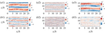
Figure 10 compares the instantaneous velocity fluctuations in an $x$ – $z$ plane at $y/h=0.12$ in the Langmuir turbulence (case $1$ ) with those in the shear-driven turbulence (case $9$ ). The contours of $u^{\prime }$ in the shear-driven turbulence show large-scale streaks with spanwise length scale $5.6h$ , accompanied by smaller-scale streaks (figure 10 b1). The contours of $u^{\prime }$ in the Langmuir turbulence are more coherent and mainly dominated by large-scale streaks with spanwise length scale $8\unicode[STIX]{x03C0}h/3$ agreeing with those of LCs (figure 10 a1), indicating the important contribution of LCs to the streamwise velocity fluctuations. This observation is similar to that of Tejada-Martínez & Grosch (Reference Tejada-Martínez and Grosch2007) at the centre of the water column at $Re_{\unicode[STIX]{x1D70F}}=395$ . Similarly, the comparison between figures 10(a3) and 10(b3) indicates that the spanwise velocity fluctuation $w^{\prime }$ is more coherent in the Langmuir turbulence than in the shear-driven turbulence. For the vertical velocity fluctuations, two negative streamwise-elongated streaks with spanwise separation of $8\unicode[STIX]{x03C0}h/3$ appear in the Langmuir turbulence (figure 10 a2), which are the footprints of the strong downwelling motions of LCs near the bottom. In contrast, the large-scale motion in the shear-driven turbulence is not sufficiently strong to leave footprints in $v^{\prime }$ near the water bottom.

4.2 Reynolds shear stress

According to (2.9), the mean velocity $\langle u\rangle$ and Reynolds shear stress $-\langle u^{\prime }v^{\prime }\rangle$ in the shallow-water Langmuir turbulence are related by the following balance equation of the mean streamwise shear stress

(4.1) $$\begin{eqnarray}\frac{\text{d}\langle u\rangle ^{+}}{\text{d}y^{+}}-\langle u^{\prime }v^{\prime }\rangle ^{+}=1.\end{eqnarray}$$

Here, the mean SGS shear stress $\langle \unicode[STIX]{x1D70F}_{12}^{sgs}\rangle$ in (2.9) is neglected, because its magnitude is negligibly small in comparison with $-\langle u^{\prime }v^{\prime }\rangle$ (figure 3). In this section, the reappearance of the logarithmic layer at $Re_{\unicode[STIX]{x1D70F}}=1000$ and the effects of $kh$ and $La_{t}$ on the thickness of the logarithmic layer are further studied through the analysis of the Reynolds shear stress.

Figure 11.

Profiles of $-\langle u^{\prime }v^{\prime }\rangle ^{+}$ in cases $1$ , $3$ and $9$ and comparison with $1-1/(\unicode[STIX]{x1D705}y^{+})$ . LCs are present in cases $1$ and $3$ with $Re_{\unicode[STIX]{x1D70F}}=1000$ and $395$ , respectively, while LCs are absent in case $9$ with $Re_{\unicode[STIX]{x1D70F}}=1000$ .

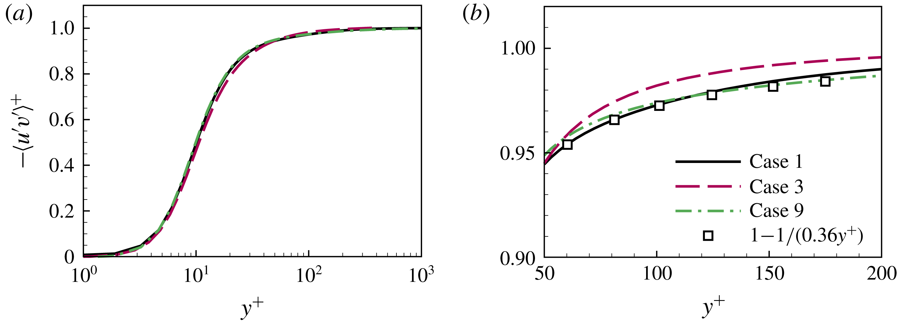
Figure 11(a) compares the profiles of $-\langle u^{\prime }v^{\prime }\rangle ^{+}$ in cases 1 and 3 for Langmuir turbulence at $Re_{\unicode[STIX]{x1D70F}}=1000$ and 395, respectively, with the result of case 9 for shear-driven turbulence superimposed. Figure 11(b) provides a zoom-in view of their distributions in the logarithmic layer. In all of these three cases, the value of $-\langle u^{\prime }v^{\prime }\rangle ^{+}$ increases monotonically as $y^{+}$ increases in the near-bottom region below $y^{+}=100$ , and approaches $1.0$ in the outer layer above $y^{+}=100$ . Substituting equation (4.1) into the definition of $F$ (3.2) gives the relationship between $F$ and $-\langle u^{\prime }v^{\prime }\rangle ^{+}$ as

(4.2) $$\begin{eqnarray}F=y^{+}+y^{+}\langle u^{\prime }v^{\prime }\rangle ^{+}.\end{eqnarray}$$

According to this equation, although the difference in the profile of $-\langle u^{\prime }v^{\prime }\rangle ^{+}$ seems to be small between cases 1 and 3, it is amplified by the multiplication with $y^{+}$ to result in a more significant difference in the profile of $F$ .

To further study the effect of the Reynolds shear stress on the logarithmic layer, we depict in figure 11(b) the profile of $-\langle u^{\prime }v^{\prime }\rangle ^{+}$ in cases 1, 3 and 9 in the logarithmic layer of the shear-driven turbulence between $y^{+}=50$ and 200. According to (4.1), the identity $-\langle u^{\prime }v^{\prime }\rangle ^{+}=1-1/(ky^{+})$ holds in the logarithmic layer. Figure 11(b) shows that in case 3 for Langmuir turbulence at $Re_{\unicode[STIX]{x1D70F}}=395$ , the value of $-\langle u^{\prime }v^{\prime }\rangle ^{+}$ is larger than $1-1/(ky^{+})$ , indicating that the mean velocity deviates from the logarithmic law. In contrast, in case 1 for Langmuir turbulence at $Re_{\unicode[STIX]{x1D70F}}=1000$ , the profile of $-\langle u^{\prime }v^{\prime }\rangle ^{+}$ is close to that of $1-1/(ky^{+})$ , meaning that the logarithmic layer reappears.

Figure 12.

Profiles of $-\langle u^{T}v^{T}\rangle ^{+}$ and $-\langle u^{L}v^{L}\rangle ^{+}$ in cases 1–3 with $Re_{\unicode[STIX]{x1D70F}}=1000$ , $700$ and $395$ , respectively. (a) Profiles of $-\langle u^{T}v^{T}\rangle ^{+}$ in near-bottom coordinate $y^{+}$ , and (b), (c) profiles of $-\langle u^{L}v^{L}\rangle ^{+}$ in near-bottom coordinate $y^{+}$ and water-column coordinate $y/h$ , respectively.

The effect of LCs on the Reynolds shear stress can be further assessed through the decomposition of $-\langle u^{\prime }v^{\prime }\rangle ^{+}$ into the LC-coherent part $-\langle u^{L}v^{L}\rangle ^{+}$ and the residual part $-\langle u^{T}v^{T}\rangle ^{+}$ (2.11). Figures 12(a) and 12(b) compare respectively the profiles of $-\langle u^{T}v^{T}\rangle ^{+}$ and $-\langle u^{L}v^{L}\rangle ^{+}$ in cases 1–3 in the near-bottom coordinate $y^{+}$ , while figure 12(c) compares the profile of $-\langle u^{L}v^{L}\rangle ^{+}$ in these cases in the water-column coordinate $y/h$ to further study the effect of the Reynolds number on the Reynolds shear stress. From the comparison between figures 12(a) and 12(b), it can be observed that the residual part $-\langle u^{T}v^{T}\rangle ^{+}$ is dominant below $y^{+}=100$ , while the LC-coherent part $-\langle u^{L}v^{L}\rangle ^{+}$ is more important above $y^{+}=100$ , consistent with the observations of Tejada-Martínez & Grosch (Reference Tejada-Martínez and Grosch2007) and Sinha et al. (Reference Sinha, Tejada-Martínez, Akan and Grosch2015). Figure 12(a) shows that, as the Reynolds number increases, the peak location of $-\langle u^{T}v^{T}\rangle ^{+}$ remains almost unchanged in the near-bottom coordinate. Different from $-\langle u^{T}v^{T}\rangle ^{+}$ , the peaks of $-\langle u^{L}v^{L}\rangle ^{+}$ are collocated in the water-column coordinate at $y/h=0.5$ (figure 12 c). Note that the near-bottom and water-column coordinates are related by the Reynolds number as $y^{+}=Re_{\unicode[STIX]{x1D70F}}y/h$ . As a result, the peaks of $-\langle u^{L}v^{L}\rangle ^{+}$ collocated at the same value of $y/h$ correspond to an increasing value of $y^{+}$ as the Reynolds number increases (figure 12 b). This indicates a weaker influence of LCs on the momentum transfer near the water bottom at higher Reynolds number, characterized by the smaller magnitude of $-\langle u^{L}v^{L}\rangle ^{+}$ below $y^{+}=200$ (figure 12 b). This effect of Reynolds number leads to the reappearance of the logarithmic layer in the near-bottom region at $Re_{\unicode[STIX]{x1D70F}}=1000$ (figure 7).

Figure 13 shows the effects of $kh$ and $La_{t}$ on the LC-coherent Reynolds shear stress $-\langle u^{L}v^{L}\rangle ^{+}$ . As depicted in figure 13(a), as the value of $kh$ increases, the peak of $-\langle u^{L}v^{L}\rangle ^{+}$ shifts to larger $y^{+}$ , and the magnitude of $-\langle u^{L}v^{L}\rangle ^{+}$ decreases below $y^{+}=200$ . This indicates a weaker effect of LCs on the momentum transfer in the near-bottom region at larger value of $kh$ . As a result, the logarithmic layer expands as the value of $kh$ increases (figure 8).

Figure 13.

Profiles of $-\langle u^{L}v^{L}\rangle ^{+}$ in (a) cases 1 and 4–6 with $kh=0.5$ , $1$ , $1.5$ and $2$ , respectively, and (b) cases 1, 7 and 8 with $La_{t}=0.7$ , $0.4$ and $0.9$ , respectively.

The magnitude of $-\langle u^{L}v^{L}\rangle ^{+}$ is non-monotonic with the increase of $La_{t}$ . As shown in figure 13(b), the magnitude of $-\langle u^{L}v^{L}\rangle ^{+}$ at $La_{t}=0.7$ is larger than those at $La_{t}=0.4$ and 0.9 between $y^{+}=20$ and $1000$ . The larger magnitude of $-\langle u^{L}v^{L}\rangle ^{+}$ at $La_{t}=0.7$ than at $La_{t}=0.9$ can be attributed to the stronger intensity of LCs due to the larger magnitude of vortex force at smaller value of $La_{t}$ (2.2). The magnitude of $-\langle u^{L}v^{L}\rangle ^{+}$ is smaller at $La_{t}=0.4$ than at $La_{t}=0.7$ , indicating a less important contribution of LCs to the momentum transfer at $La_{t}=0.4$ , which is consistent with the observation of Sinha et al. (Reference Sinha, Tejada-Martínez, Akan and Grosch2015) at $Re_{\unicode[STIX]{x1D70F}}=395$ . As explained by Sinha et al. (Reference Sinha, Tejada-Martínez, Akan and Grosch2015), the intensities of the upwelling motion induced by LCs become stronger at a smaller value of $La_{t}$ due to the larger magnitude of C–L vortex forcing. The strong upwelling motion at $La_{t}=0.4$ shifts LCs towards the water surface. As a result, the magnitude of the LC-coherent Reynolds stress is smaller at $La_{t}=0.4$ than at $La_{t}=0.7$ in the lower half of the water column. The residual turbulence motions become important in the momentum transfer at $La_{t}=0.4$ , which is indicated by $-\langle u^{T}v^{T}\rangle ^{+}$ . To further study the effects of $La_{t}$ on the residual turbulence motions, we compare $-\langle u^{T}v^{T}\rangle ^{+}$ among cases 1, 7 and 8 in figure 14(a), and the pre-multiplied spanwise co-spectrum $\unicode[STIX]{x1D719}_{uv}^{T}(y,k_{z})=k_{z}E_{uv}^{T}(y,k_{z})$ at a near-bottom plane $y^{+}=120$ and a water-column central plane $y/h=1.0$ in figures 14(b) and 14(c), respectively. Here, $k_{z}=2\unicode[STIX]{x03C0}/\unicode[STIX]{x1D706}_{z}$ is the spanwise wavenumber corresponding to the spanwise length scale $\unicode[STIX]{x1D706}_{z}$ , and $E_{uv}^{T}(y,k_{z})$ is the spanwise co-spectrum between $u^{T}$ and $v^{T}$ , which satisfies the normalization property

(4.3) $$\begin{eqnarray}\langle u^{T}v^{T}\rangle (y)=\int _{0}^{\infty }E_{uv}^{T}(y,k_{z})\,\text{d}k_{z}=\int _{-\infty }^{+\infty }k_{z}E_{uv}^{T}(y,k_{z})\,\text{d}\log (k_{z}).\end{eqnarray}$$

Figure 14.

Residual part of Reynolds shear stress $-\langle u^{T}v^{T}\rangle ^{+}$ and pre-multiplied co-spectrum $-\unicode[STIX]{x1D719}_{uv}^{T}$ in cases 1, 7 and 8 with $La_{t}=0.7$ , $0.4$ and $0.9$ , respectively. (a) Profiles of $-\langle u^{T}v^{T}\rangle ^{+}$ , (b) pre-multiplied co-spectra $-\unicode[STIX]{x1D719}_{uv}^{T}$ at $y^{+}=120$ and (c) pre-multiplied co-spectra $-\unicode[STIX]{x1D719}_{uv}^{T}$ at $y/h=1$ .

As shown in figure 14(a), the magnitude of the residual turbulence part of Reynolds shear stress $-\langle u^{T}v^{T}\rangle ^{+}$ is larger at $La_{t}=0.4$ than at $La_{t}=0.7$ above $y^{+}=20$ and $La_{t}=0.9$ above $y^{+}=100$ , which results from the intensification of residual turbulence motions. The effect of turbulence motions on $-\langle u^{T}v^{T}\rangle ^{+}$ can be observed from the pre-multiplied spanwise co-spectrum $-\unicode[STIX]{x1D719}_{uv}^{T}$ shown in figure 14(b,c). At the near-bottom plane $y^{+}=120$ (figure 14 b), the magnitude of $-\unicode[STIX]{x1D719}_{uv}^{T}$ at $La_{t}=0.4$ is larger than that at $La_{t}=0.7$ for $\unicode[STIX]{x1D706}_{z}^{+}>200$ , indicating that the larger magnitude of $-\langle u^{T}v^{T}\rangle ^{+}$ at $La_{t}=0.4$ results from the enhancement of the large-scale turbulence motions ( $\unicode[STIX]{x1D706}_{z}^{+}>200$ ). Akan et al. (Reference Akan, Tejada-Martínez, Grosch and Martinat2013) and Sinha et al. (Reference Sinha, Tejada-Martínez, Akan and Grosch2015) pointed out that the strong shear of Stokes drift at $La_{t}=0.4$ significantly enhances the large-scale turbulent motion in the vertical direction in the upper half of the water column. It is evident from figure 14(c) that the large-scale turbulent motions also lead to the magnitude increase of $-\unicode[STIX]{x1D719}_{uv}^{T}$ at spanwise scales larger than $\unicode[STIX]{x1D706}_{z}^{+}=200$ at the centre of the water column $y/h=1$ . By comparing figure 14(b) with figure 14(c), it is observed that as the value of $La_{t}$ decreases from $0.7$ to $0.4$ , the magnitude of $-\unicode[STIX]{x1D719}_{uv}^{T}$ increases at the same spanwise scales ( $\unicode[STIX]{x1D706}_{z}^{+}>200$ ). This indicates that the large-scale turbulent motions are sufficiently strong to reach the near-bottom region. As a result, the magnitude of $-\langle u^{T}v^{T}\rangle$ also becomes stronger at $La_{t}=0.4$ than at $La_{t}=0.7$ near the water bottom. This effect of large-scale turbulence motion on the near-bottom momentum flux is absent at larger value of $La_{t}$ , because of the smaller Stokes shear. As shown in figure 14(b), the magnitude of $-\unicode[STIX]{x1D719}_{uv}^{T}$ is larger at $La_{t}=0.9$ than at $La_{t}=0.7$ at all spanwise scales $\unicode[STIX]{x1D706}_{z}^{+}$ . In contrast, as shown in figure 14(c), at $y/h=1$ , the magnitudes of $-\unicode[STIX]{x1D719}_{uv}^{T}$ at $La_{t}=0.9$ and 0.7 are comparable at most spanwise scales except for $\unicode[STIX]{x1D706}_{z}^{+}\geqslant 7000$ . This indicates that the suppression of $-\langle u^{T}v^{T}\rangle ^{+}$ near the water bottom in response to the decrease of $La_{t}$ from 0.9 to 0.7 cannot be attributed to large-scale turbulence motions at $y/h=1$ . Martinat et al. (Reference Martinat, Grosch and Gatski2014) and Sinha et al. (Reference Sinha, Tejada-Martínez, Akan and Grosch2015) pointed out that LCs tend to suppress the momentum flux induced by turbulent motions. Because the impact of LCs on the momentum flux near the bottom is weaker at $La_{t}=0.9$ than at $La_{t}=0.7$ (figure 13 b), the magnitude of $-\langle u^{T}v^{T}\rangle ^{+}$ becomes larger as $La_{t}$ increases from $0.7$ to $0.9$ .

4.3 Reynolds normal stresses

Figure 15.

Profiles of $\langle u^{\prime }u^{\prime }\rangle ^{+}$ in the coordinate of (a) $y^{+}$ and (b) $y/h$ in cases 1–3 with $Re_{\unicode[STIX]{x1D70F}}=1000$ , $700$ and $395$ , respectively. In (a), the line with open circles represents the result in case $9$ (the shear-driven turbulence at $Re_{\unicode[STIX]{x1D70F}}=1000$ ) as a reference.

We start our analyses of Reynolds normal stresses with the effect of the Reynolds number. Figure 15 compares the profiles of $\langle u^{\prime }u^{\prime }\rangle ^{+}$ among cases 1–3 with different Reynolds numbers. The result of case 9 for shear-driven turbulence is superimposed for comparison. As shown in figure 15(a), at $Re_{\unicode[STIX]{x1D70F}}=395$ , there is a single peak in the profile of $\langle u^{\prime }u^{\prime }\rangle ^{+}$ . This peak is located at $y^{+}=32$ , different from the peak location of $\langle u^{\prime }u^{\prime }\rangle ^{+}$ at $y^{+}=11$ in the shear-driven turbulence. As the Reynolds number increases to 700 and 1000, the profile of $\langle u^{\prime }u^{\prime }\rangle ^{+}$ shows a bimodal shape. As shown in figure 15(a), the inner peak at $y^{+}=12$ is close to that in the shear-driven turbulence. Although an outer peak of $\langle u^{\prime }u^{\prime }\rangle ^{+}$ also occurs in canonical wall-bounded turbulence for $Re_{\unicode[STIX]{x1D70F}}>15\,000$  (Alfredsson, Segalini & Örlü Reference Alfredsson, Segalini and Örlü2011), the one in Langmuir turbulence is different in three aspects. First, the outer peak of $\langle u^{\prime }u^{\prime }\rangle ^{+}$ in the Langmuir turbulence occurs at a much smaller Reynolds number of 700. Second, in the shallow-water Langmuir turbulence, the outer peak location is scaled by $h$ for various Reynolds numbers. As shown in figure 15(b), at $Re_{\unicode[STIX]{x1D70F}}=700$ and $1000$ , the outer peak of $\langle u^{\prime }u^{\prime }\rangle ^{+}$ is collocated at $y/h=0.11$ . However, the outer peak in the canonical wall-bounded turbulence for $Re_{\unicode[STIX]{x1D70F}}>15\,000$ is located at $y^{+}\sim Re_{\unicode[STIX]{x1D70F}}^{1/2}$  (Alfredsson et al. Reference Alfredsson, Segalini and Örlü2011). Third, as shown in figure 15(b), in the water-column coordinate $y/h$ , the profiles of $\langle u^{\prime }u^{\prime }\rangle ^{+}$ in the outer layer of the Langmuir turbulence at various Reynolds numbers are close to each other. In contrast, in the canonical wall-bounded turbulence, the profiles of $\langle u^{\prime }u^{\prime }\rangle ^{+}$ at various Reynolds numbers deviate from each other in the outer coordinate $y/h$  (Hoyas & Jiménez Reference Hoyas and Jiménez2006; Avsarkisov et al. Reference Avsarkisov, Hoyas, Oberlack and Garcia-Galache2014; Bernardini et al. Reference Bernardini, Pirozzoli and Orlandi2014; Lee & Moser Reference Lee and Moser2015). It is evident from the above three points that the occurrence of LCs significantly alters the profile of $\langle u^{\prime }u^{\prime }\rangle ^{+}$ .

Figure 16.

Profiles of $\langle v^{\prime }v^{\prime }\rangle ^{+}$ in the coordinate of (a) $y^{+}$ and (b) $y/h$ in cases 1–3 with $Re_{\unicode[STIX]{x1D70F}}=1000$ , $700$ and $395$ , respectively. In (a), the line with open circles represents the result in case $9$ (the shear-driven turbulence at $Re_{\unicode[STIX]{x1D70F}}=1000$ ) as a reference.

Figure 16 shows the Reynolds number effect on the profiles of $\langle v^{\prime }v^{\prime }\rangle ^{+}$ . As shown in figure 16(a), the value of $\langle v^{\prime }v^{\prime }\rangle ^{+}$ increases monotonically with $y^{+}$ at $Re_{\unicode[STIX]{x1D70F}}=395$ . In contrast, at $Re_{\unicode[STIX]{x1D70F}}=700$ and $1000$ , a local peak located at $y^{+}=50$ occurs in the profile of $\langle v^{\prime }v^{\prime }\rangle ^{+}$ . As the distance from the bottom further increases, the profiles of $\langle v^{\prime }v^{\prime }\rangle ^{+}$ at $Re_{\unicode[STIX]{x1D70F}}=700$ and $1000$ first reach their local minimal values at $y/h\approx 0.17$ , and then increases again with $y/h$ (figure 16 b). The shape of the $\langle v^{\prime }v^{\prime }\rangle ^{+}$ profile in shallow-water Langmuir turbulence is drastically different from that in the shear-driven turbulence and canonical wall-bounded turbulence (Kim, Moin & Moser Reference Kim, Moin and Moser1987; Hoyas & Jiménez Reference Hoyas and Jiménez2006; Avsarkisov et al. Reference Avsarkisov, Hoyas, Oberlack and Garcia-Galache2014; Bernardini et al. Reference Bernardini, Pirozzoli and Orlandi2014; Lee & Moser Reference Lee and Moser2015). For example, the value of $\langle v^{\prime }v^{\prime }\rangle ^{+}$ in the turbulent Couette flow (Avsarkisov et al. Reference Avsarkisov, Hoyas, Oberlack and Garcia-Galache2014) and the shear-driven turbulence is close to a constant in the outer layer, while in the pressure-driven turbulent channel flow the magnitude of $\langle v^{\prime }v^{\prime }\rangle ^{+}$ decreases with $y^{+}$ in the outer layer (Kim et al. Reference Kim, Moin and Moser1987; Hoyas & Jiménez Reference Hoyas and Jiménez2006; Lee & Moser Reference Lee and Moser2015).

Figure 17.

Profiles of $\langle w^{\prime }w^{\prime }\rangle ^{+}$ in the coordinate of (a) $y^{+}$ and (b) $y/h$ in cases 1–3 with $Re_{\unicode[STIX]{x1D70F}}=1000$ , $700$ and $395$ , respectively. In (a), the line with open circles represents the result in case $9$ (the shear-driven turbulence at $Re_{\unicode[STIX]{x1D70F}}=1000$ ) as a reference.

Figure 17 compares the profiles of $\langle w^{\prime }w^{\prime }\rangle ^{+}$ in shallow-water Langmuir turbulence at various Reynolds numbers. Figure 17(a) shows that in the wall coordinate $y^{+}$ , the magnitude of $\langle w^{\prime }w^{\prime }\rangle ^{+}$ increases as the Reynolds number increases. In Langmuir turbulence at $Re_{\unicode[STIX]{x1D70F}}=395$ , 700 and 1000, the peak value of $\langle w^{\prime }w^{\prime }\rangle ^{+}$ is respectively $5.7$ , $6.6$ and $7.2$ , significantly larger than those in the shear-driven turbulence (figure 17 a) and canonical wall-bounded turbulence at $Re_{\unicode[STIX]{x1D70F}}\leqslant 1000$  (approximately 2.0–3.0, see e.g. Kim et al. Reference Kim, Moin and Moser1987; Hoyas & Jiménez Reference Hoyas and Jiménez2006; Avsarkisov et al. Reference Avsarkisov, Hoyas, Oberlack and Garcia-Galache2014; Bernardini et al. Reference Bernardini, Pirozzoli and Orlandi2014). The peak location of $\langle w^{\prime }w^{\prime }\rangle ^{+}$ in Langmuir turbulence is also different from that in shear-driven turbulence and canonical wall-bounded turbulence. In Langmuir turbulence, the peak location of $\langle w^{\prime }w^{\prime }\rangle ^{+}$ is scaled by $h$ . As shown in figure 17(b), the peaks of $\langle w^{\prime }w^{\prime }\rangle ^{+}$ at various Reynolds numbers collocate at $y/h=0.15$ . In canonical wall-bounded turbulence, the peak of $\langle w^{\prime }w^{\prime }\rangle ^{+}$ is located at $y^{+}=30{-}40$  (Kim et al. Reference Kim, Moin and Moser1987; Hoyas & Jiménez Reference Hoyas and Jiménez2006; Avsarkisov et al. Reference Avsarkisov, Hoyas, Oberlack and Garcia-Galache2014; Bernardini et al. Reference Bernardini, Pirozzoli and Orlandi2014), closer to the wall than in Langmuir turbulence. Similarly, in the shear-driven turbulence the peak is located at $y^{+}=30$ (figure 17 a). From the comparison of the peak magnitude and location of $\langle u^{\prime }u^{\prime }\rangle ^{+}$ , $\langle v^{\prime }v^{\prime }\rangle ^{+}$ and $\langle w^{\prime }w^{\prime }\rangle ^{+}$ between the shallow-water Langmuir turbulence and canonical wall turbulence without LCs, it is evident that LCs make a substantial contribution to the Reynolds normal stresses in Langmuir turbulence.

Figure 18.

Profiles of (a) $\langle u^{L}u^{L}\rangle ^{+}$ in the coordinate of $y/h$ , (b) $\langle u^{L}u^{L}\rangle ^{+}$ and (c) $\langle u^{T}u^{T}\rangle ^{+}$ in the coordinate of $y^{+}$ in cases  $1$ – $3$ with $Re_{\unicode[STIX]{x1D70F}}=1000$ , $700$ and $395$ , respectively.

Similar to the analyses of Reynolds shear stress in § 4.2, we employ the decomposition of the Reynolds stress (2.11) to study the effect of LCs on the Reynolds normal stresses in Langmuir turbulence at various Reynolds numbers. Figure 18 shows the profiles of $\langle u^{L}u^{L}\rangle ^{+}$ and $\langle u^{T}u^{T}\rangle ^{+}$ , while figures 19 and 20 show respectively those of $\langle v^{L}v^{L}\rangle ^{+}$ and $\langle v^{T}v^{T}\rangle ^{+}$ and those of $\langle w^{L}w^{L}\rangle ^{+}$ and $\langle w^{T}w^{T}\rangle ^{+}$ at various Reynolds numbers. In each of these three figures, the left column compares the profiles of LC-coherent part in the water-column coordinate, while the middle and right columns compare respectively the profiles of LC-coherent and residual parts in the near-bottom coordinate.

From the comparison among figures 15–20, it can be observed that in the outer layer, all of the three LC-coherent Reynolds normal stresses make important contributions to the total Reynolds normal stresses, which is consistent with the observations of Tejada-Martínez & Grosch (Reference Tejada-Martínez and Grosch2007) and Sinha et al. (Reference Sinha, Tejada-Martínez, Akan and Grosch2015) at $Re_{\unicode[STIX]{x1D70F}}=395$ . Figure 18(a) shows that the location of the $\langle u^{L}u^{L}\rangle ^{+}$ peak is scaled by $h$ . The peaks of $\langle u^{L}u^{L}\rangle ^{+}$ at various Reynolds numbers collocate at $y/h=0.11$ , which is consistent with the outer peak of $\langle u^{\prime }u^{\prime }\rangle ^{+}$ at $Re_{\unicode[STIX]{x1D70F}}=700$ and $1000$ (figure 15 b). From the comparison between figures 18(b) and 18(c), it can be observed that the magnitude of $\langle u^{L}u^{L}\rangle ^{+}$ is much larger than that of $\langle u^{T}u^{T}\rangle ^{+}$ above $y^{+}=100$ , indicating that the outer peaks of $\langle u^{\prime }u^{\prime }\rangle ^{+}$ at $Re_{\unicode[STIX]{x1D70F}}=700$ and 1000 are induced by the LCs. Figure 19(b) shows that the value of $\langle v^{L}v^{L}\rangle ^{+}$ increases with $y^{+}$ in the outer layer. In contrast, as depicted in figure 19(c), the profile of $\langle v^{T}v^{T}\rangle ^{+}$ is relatively flat above $y^{+}=100$ . This indicates that the increase of $\langle v^{\prime }v^{\prime }\rangle ^{+}$ with $y^{+}$ above $y^{+}=100$ (figure 16 b) is caused by the LCs. Similar to $\langle u^{L}u^{L}\rangle ^{+}$ , the peak location of $\langle w^{L}w^{L}\rangle ^{+}$ is scaled by $h$ at various Reynolds numbers. As shown in figure 20(a), the peaks of $\langle w^{L}w^{L}\rangle ^{+}$ at various Reynolds numbers collocate at $y/h=0.16$ , which are close to those of $\langle w^{\prime }w^{\prime }\rangle ^{+}$ at $y/h=0.15$ (figure 17 b). In contrast, as shown in figure 20(c), the magnitude of the $\langle w^{T}w^{T}\rangle ^{+}$ profile changes little with $y^{+}$ . Therefore, the peak of $\langle w^{\prime }w^{\prime }\rangle ^{+}$ in the shallow-water Langmuir turbulence results from the contribution of LCs.

Figure 19.

Profiles of (a) $\langle v^{L}v^{L}\rangle ^{+}$ in the coordinate of $y/h$ , (b) $\langle v^{L}v^{L}\rangle ^{+}$ and (c) $\langle v^{T}v^{T}\rangle ^{+}$ in the coordinate of $y^{+}$ in cases  $1$ – $3$ with $Re_{\unicode[STIX]{x1D70F}}=1000$ , $700$ and $395$ , respectively.

Figure 20.

Profiles of (a) $\langle w^{L}w^{L}\rangle ^{+}$ in the coordinate of $y/h$ , (b) $\langle w^{L}w^{L}\rangle ^{+}$ and (c) $\langle w^{T}w^{T}\rangle ^{+}$ in the coordinate of $y^{+}$ in cases  $1$ – $3$ with $Re_{\unicode[STIX]{x1D70F}}=1000$ , $700$ and $395$ , respectively.

In the near-bottom region below $y^{+}=100$ , it can be observed from the comparisons between figures 18(b) and 18(c), and between figures 20(b) and 20(c) that the magnitudes of $\langle u^{L}u^{L}\rangle ^{+}$ and $\langle w^{L}w^{L}\rangle ^{+}$ are comparable to those of $\langle u^{T}u^{T}\rangle ^{+}$ and $\langle w^{T}w^{T}\rangle ^{+}$ , respectively. This indicates that both the LC-coherent and residual parts are important to the total Reynolds normal stresses $\langle u^{\prime }u^{\prime }\rangle$ and $\langle w^{\prime }w^{\prime }\rangle$ near the bottom. As shown in figure 18(c), the peaks of $\langle u^{T}u^{T}\rangle ^{+}$ at various Reynolds numbers collocate at $y^{+}=12$ . At $Re_{\unicode[STIX]{x1D70F}}=395$ , because the peak of $\langle u^{T}u^{T}\rangle ^{+}$ is close to that of $\langle u^{L}u^{L}\rangle ^{+}$ , neither of them alone is shown in the profile of the total Reynolds normal stress $\langle u^{\prime }u^{\prime }\rangle$ (figure 15 a). As the Reynolds number increases, the peak of $\langle u^{T}u^{T}\rangle ^{+}$ is located at the same $y^{+}$ , but that of $\langle u^{L}u^{L}\rangle ^{+}$ moves to larger $y^{+}$ . As a result, the peaks of both $\langle u^{T}u^{T}\rangle ^{+}$ and $\langle u^{L}u^{L}\rangle$ are shown in the profile of $\langle u^{\prime }u^{\prime }\rangle$ , forming a bimodal shape (figure 15 a). The peak of $\langle w^{T}w^{T}\rangle ^{+}$ for various Reynolds numbers collocates at $y^{+}=30$ , where its magnitude is smaller than that of $\langle w^{L}w^{L}\rangle ^{+}$ . As a result, the peak of $\langle w^{T}w^{T}\rangle ^{+}$ is not shown in the profile of $\langle w^{\prime }w^{\prime }\rangle$ (figure 17 a). From the comparison between figure 17(a) and figure 20(b), it can be deduced that the single peak of $\langle w^{\prime }w^{\prime }\rangle$ is induced by the LC-coherent part $\langle w^{L}w^{L}\rangle ^{+}$ . The peak locations of $\langle w^{\prime }w^{\prime }\rangle$ and $\langle w^{L}w^{L}\rangle ^{+}$ are close to each other. As the Reynolds number increases, they both shift away from the bottom, with their magnitude increasing.

Different from $\langle u^{L}u^{L}\rangle ^{+}$ and $\langle w^{L}w^{L}\rangle ^{+}$ , the magnitude of $\langle v^{L}v^{L}\rangle ^{+}$ is much smaller than that of $\langle v^{T}v^{T}\rangle ^{+}$ near the water bottom (figure 19 b,c). In wall-bounded turbulent flows, the vertical mixing is responsible for the generation of Reynolds shear stresses (Blackwelder & Eckelmann Reference Blackwelder and Eckelmann1979; Robinson Reference Robinson1991; Jeong et al. Reference Jeong, Hussain, Schoppa and Kim1997; Jiménez & Pinelli Reference Jiménez and Pinelli1999; Panton Reference Panton2001). As a result, the magnitude of $-\langle u^{L}v^{L}\rangle ^{+}$ is also small in the near-bottom region (figure 12 b). As the Reynolds number increases, the profile of $\langle v^{L}v^{L}\rangle ^{+}$ shifts to larger $y^{+}$ , leading to the thickness increase of the near-bottom region with a small magnitude of $\langle v^{L}v^{L}\rangle ^{+}$ . In response, the near-bottom region with a small magnitude of $-\langle u^{L}v^{L}\rangle ^{+}$ also becomes thicker at higher Reynolds number, which in turn leads to the reappearance of the logarithmic layer at $Re_{\unicode[STIX]{x1D70F}}=1000$ .

Figure 21.

Profiles of (a1) $\langle u^{\prime }u^{\prime }\rangle ^{+}$ , (a2) $\langle u^{L}u^{L}\rangle ^{+}$ , (a3) $\langle u^{T}u^{T}\rangle ^{+}$ , (b1) $\langle v^{\prime }v^{\prime }\rangle ^{+}$ , (b2) $\langle v^{L}v^{L}\rangle ^{+}$ , (b3) $\langle v^{T}v^{T}\rangle ^{+}$ , (c1) $\langle w^{\prime }w^{\prime }\rangle ^{+}$ , (c2) $\langle w^{L}w^{L}\rangle ^{+}$ and (c3) $\langle w^{T}w^{T}\rangle ^{+}$ in cases $1$ and $4-6$ with $kh=0.5$ , $1$ , $1.5$ and $2$ , respectively.

Figure 21 shows the effects of $kh$ on the Reynolds normal stresses, together with their LC-coherent parts and the residual turbulence parts. As the value of $kh$ increases, the profile of Stokes drift velocity in (2.4) shifts towards the water surface, and the magnitude of vortex force term in the C–L equations (2.2) is suppressed in the bottom half of the water column, which weakens the intensity of LCs. In response, the profiles of the LC-coherent Reynolds normal stresses shift towards the water surface (figure 21 a2,b2,c2), with the magnitude of the $\langle u^{L}u^{L}\rangle ^{+}$ peak decreasing slightly (figure 21 a2) and those of $\langle v^{L}v^{L}\rangle ^{+}$ and $\langle w^{L}w^{L}\rangle ^{+}$ decreasing throughout the bottom half of the water column (figure 21 b2,c2). The present observation of the effects of $kh$ on the intensity of LCs is consistent with that of Tejada-Martínez et al. (Reference Tejada-Martínez, Grosch, Sinha, Akan and Martinat2012) and Sinha et al. (Reference Sinha, Tejada-Martínez, Akan and Grosch2015) at $Re_{\unicode[STIX]{x1D70F}}=395$ . The smaller magnitude of $\langle v^{L}v^{L}\rangle ^{+}$ indicates weaker vertical turbulence mixing coherent to the motion of LCs, such that the magnitude of $-\langle u^{L}v^{L}\rangle ^{+}$ decreases as the value of $kh$ increases (figure 13 a), resulting in the wider logarithmic layer at larger value of $kh$ (figure 8).

In the outer layer, because the turbulence is dominated by the LCs, the effects of $kh$ on the Reynolds normal stresses are dominated by those on their LC-coherent parts. This is evident by comparing figures 21(a1), 21(b1), 21(c1) with figures 21(a2), 21(b2) and 21(c2), respectively. From the comparison, it can be observed that above $y^{+}=200$ , the effects of $kh$ on the total Reynolds normal stresses are consistent with those on their LC-coherent part.

In the near-bottom region with $y^{+}<20$ , the profiles of $\langle u^{T}u^{T}\rangle$ , $\langle v^{T}v^{T}\rangle$ and $\langle w^{T}w^{T}\rangle$ are barely influenced by $kh$ (figure 21 a3,b3,c3), indicating that the interaction between LCs and residual turbulence is week and the residual turbulence is not significantly influenced by the reduction in LC intensity. However, because the LC-coherent motion makes a considerable contribution to $\langle u^{\prime }u^{\prime }\rangle$ and $\langle w^{\prime }w^{\prime }\rangle$ in the inner layer (figure 21 a2,c2), the magnitudes of $\langle u^{\prime }u^{\prime }\rangle$ and $\langle w^{\prime }w^{\prime }\rangle$ decrease in the inner layer as the value of $kh$ increases. As shown in figures 21(a1) and 21(c1), the LC-coherent motion influences the profiles of $\langle u^{\prime }u^{\prime }\rangle$ and $\langle w^{\prime }w^{\prime }\rangle$ down to $y^{+}=10$ and $y^{+}=4$ , respectively. Different from $\langle u^{L}u^{L}\rangle$ and $\langle w^{L}w^{L}\rangle$ , the magnitude of $\langle v^{L}v^{L}\rangle$ is negligibly small in the inner layer below $y^{+}=100$ (figure 21 b2), such that the effect of $kh$ on $\langle v^{\prime }v^{\prime }\rangle$ is consistent with that on $\langle v^{T}v^{T}\rangle$ . As shown in figure 21(b1,b3), between $y^{+}=40$ and $100$ , the magnitudes of $\langle v^{\prime }v^{\prime }\rangle$ and $\langle v^{T}v^{T}\rangle$ both increase slightly as the value of $kh$ increases.

Figure 22.

Profiles of (a1) $\langle u^{\prime }u^{\prime }\rangle ^{+}$ , (a2) $\langle u^{L}u^{L}\rangle ^{+}$ , (a3) $\langle u^{T}u^{T}\rangle ^{+}$ , (b1) $\langle v^{\prime }v^{\prime }\rangle ^{+}$ , (b2) $\langle v^{L}v^{L}\rangle ^{+}$ , (b3) $\langle v^{T}v^{T}\rangle ^{+}$ , (c1) $\langle w^{\prime }w^{\prime }\rangle ^{+}$ , (c2) $\langle w^{L}w^{L}\rangle ^{+}$ and (c3) $\langle w^{T}w^{T}\rangle ^{+}$ in cases 1, 7 and 8 with $La_{t}=0.7$ , $0.4$ and $0.9$ , respectively.

Figure 22 shows the effect of $La_{t}$ on the profiles of the Reynolds normal stresses, their LC-coherent parts, and residual parts. Similar to the LC-coherent Reynolds shear stress discussed in § 4.2, the magnitudes of the LC-coherent Reynolds normal stresses are not monotonic with the increase of $La_{t}$ . As shown in figure 22(a2,b2,c2), the magnitudes of $\langle u^{L}u^{L}\rangle ^{+}$ , $\langle v^{L}v^{L}\rangle ^{+}$ and $\langle w^{L}w^{L}\rangle ^{+}$ are all larger at $La_{t}=0.7$ than at 0.4 and 0.9, indicating that the intensity of the LCs reverses at $La_{t}=0.7$ . Further because the residual parts of the Reynolds normal stresses $\langle u^{T}u^{T}\rangle ^{+}$ and $\langle w^{T}w^{T}\rangle ^{+}$ are not significantly influenced by the value of $La_{t}$ (figure 22 a3,c3), the magnitudes of $\langle u^{\prime }u^{\prime }\rangle ^{+}$ and $\langle w^{\prime }w^{\prime }\rangle ^{+}$ also reverse at $La_{t}=0.7$ (figure 22 a1,c1). In contrast, the magnitude of $\langle v^{\prime }v^{\prime }\rangle ^{+}$ is monotonic to the value increase of $La_{t}$ (figure 22 b1), due to the magnitude increase of $\langle v^{T}v^{T}\rangle ^{+}$ as the value of $La_{t}$ decreases from 0.7 to 0.4, which is also observed by Sinha et al. (Reference Sinha, Tejada-Martínez, Akan and Grosch2015) at $Re_{\unicode[STIX]{x1D70F}}=395$ .