2. The game

In Mexico, the number of children out of school is large enough to feed back into poverty as the trend of potential students out of the classroom is one of sustained increase. This applies to both out-of-school adolescents (the percentage of adolescents of lower secondary school age who are not enrolled in school) and out-of-school children (the percentage of primary school-age children who are not enrolled in primary or secondary school).Footnote ⁸

The Obligatory Schooling Standard of the Mexican State (NEOEM) establishes that the population with deprivation due to educational backwardness meets any of the following criteria: (i) he or she is between 3 and 15 years old, does not have compulsory basic education, and does not attend a formal education center; (ii) he or she was born before 1982 and does not have the level of compulsory education in force at the time he or should have completed it (complete primary school); and (iii) he or she was born in 1982 and does not have the level of compulsory education (complete secondary school). At the national level, it was observed that between 2018 and 2020, the educational gap increased by 0.3 percentage points (although this change was not statistically significant), from 19.0% to 19.2%.Footnote ⁹ The main problems of the Mexican educational system are coverage, quality, social inequity, and desertion driven by household income [Angulo-Cázares (Reference Angulo-Cázares2018)]. In this socioeconomic environment, Mexicans face the dilemma of completing their studies or not. These are the choices that a Mexican should make.

How the process of preference formation takes place in a society, for example, within the educational system, becomes an important focal point in development economics, stimulating a critical reflection on what preferences are cultivated in it. Generally, preferences can be activated, but they are stable in the short term. However, in the long term, they can change and are specific to socialization (peer effects) and culture and strongly interrelated with the educational levels of a society [Bowles (Reference Bowles1998, Reference Bowles2008)].Footnote ¹⁰ Particularly, in the following one-shot game, the strategies are those in which people or individuals choose to complete or not their levels of education (studies, training, accumulation of human capital). This is strategic simply because this action can be costly when the state of the economy makes studying or going to school unprofitable for individuals [see, e.g., Bloom et al. (Reference Bloom, Khoury, Kufenko and Prettner2021); Ceroni (Reference Ceroni2001); Sanchez Carrera (Reference Sanchez Carrera2019)].

In other words, to simplify the game, in what follows, our economy is made up of two population players consisting of individuals, agents, and/or citizens of a representative economy. These agents can be interpreted as potential employees/workers with high or low skill levels depending on their levels of education, for example. That is, the two populations can be interpreted as types of potential employees/workers who have to choose between acquiring or not skills/education levels. The general case must consider n-populations, but these two populations can be generalized. What distinguishes these two populations is simply the asymmetry in neighborhoods, or municipalities, and their compositions. Although the general case is for n-neighborhoods or n-municipalities, it is worth noting the citizens within their populations if they interact with their own kind and then through the dynamic system of the replicator to define the evolution of the entire economy. That is, there are two population agents who face each other (at random), citizen 1 against citizen 2, and have to choose between two strategies: to complete (E) or not complete (N) their educational levels. In other words, the two populations simply represent the interactions between person-populations of a certain type and person-populations of the same or another type. The types are people with complete educational levels and people with incomplete educational levels. In addition, when applying the replicator dynamics, we consider that there are pairing effects in the economy within each population and between the two populations. That is, the more agents of a certain type (i.e., with or without full education) there are within and between the two populations, the more the dynamic evolution of the economy toward one stationary state or another is affected.

We postulate matching effects in the economy: the more agents of a certain type there are, the more the corresponding payoffs to the strategies of the types of agents are impacted. There are also education costs, which can measure labor-market conditions for skilled/unskilled workers. We assume that the Mexican economy is primarily an unskilled labor market, so educational costs are present only for those agents who opt for the complete education strategy.Footnote ¹¹ The normal-form representation of this one-shot game is given by the payoff matrix:

That is, this economy is characterized by payoffs defined as follows:

• Player $i=1,2$ , who opts for the full education strategy $E_{i}$ , receives when facing a player $j\neq i=1,2$ , who instead opts for the incomplete-education strategy $N_{j}$ , player $i=1,2,$ a payoff given by:

  \begin{equation*} \pi _{i}\left(E_{i},N_{j}\right)=\alpha +bW_{i}-C_{i}\left(\cdot \right) \end{equation*}
  where $\alpha \geq 0$ is a constant value of the innate abilities (e.g., minimum or subsistence wages), the earnings (or income) from attaining education are given by $bW_{i}\gt 0$ , with $b\in [0,1]$ as the marginal effect that provides the option of a complete education (i.e., a skill premium, human capital wages, etc.).

  The costs of education for player $i$ are given by $C_{i}(\cdot )=\sigma +\beta N_{j}$ , where $N_{j}$ is the number of individuals with an incomplete education when player $i$ is different from $j$ and faces them. That is, due to neighborhood effects, education costs $C_{i}(\cdot )$ increase directly and proportionally when facing players $j$ with incomplete education, $\beta N_{j}\gt 0$ , since education costs also consider matching effects $\beta \in (0,1)$ as a weighting element.Footnote ¹² In other words, these costs increase in such a way by the assumption of either the segregation or segmentation of citizens/players/agents. This is included in the mathematical model through the measures provided by the shares of citizens/agents that are of one profile or another. In addition, by $\sigma \gt 0$ measuring baseline educational costs driven by, for example, labor-market demand conditions for unskilled labor.

• Player $i=1,2$ , who opts for the full education strategy $E_{i}$ , obtains when facing player $j\neq i=1,2$ , who also opts for strategy $E_{j}$ , a payoff:

  \begin{equation*} \pi _{i}\left(E_{i},E_{j}\right)=\alpha +bW_{i}-C_{i}\left(\cdot \right) \end{equation*}
  In this case, the costs of education, $C_{i}(\cdot )$ , are assumed to take the form:
  \begin{equation*} C_{i}\left(\cdot \right)=\sigma +\frac{\beta }{E_{j}} \end{equation*}
  where $\sigma \gt 0$ measures the baseline educational costs. Education costs also consider matching effects, which we define as inversely proportional, $\frac{\beta }{E_{j}}\gt 0,$ to the number of agents that one faces with complete education levels $E_{j}$ . This involves neighborhood effects because the greater the number of people one faces with a complete education, the less costly it will be to take the strategy/action of complete education (Barrios-Fernández Reference Barrios-Fernández2022).Footnote ¹³ Hence, synergies are considered in this case, in which one person with a complete education faces another with a complete education: the positive synergies decrease the costs of education as there are always more people with a complete education.

• Player $i=1,2$ , who opts for the incomplete-education strategy $N_{i}$ , receives when facing a player $j\neq i=1,2$ , who instead opts for the complete-education strategy $E_{j}$ , a payoff:

  \begin{equation*} \pi _{i}\left(N_{i}, E_{j}\right)=\alpha +\beta E_{j} \end{equation*}
  That is, when player $i$ opts for the incomplete education strategy, she/he will not obtain the income $W_{i}=0$ but does not face the costs of education either, $C_{i}(\cdot )=0$ . The only reward is derived from innate abilities $\alpha \geq 0$ and positive synergies (matching effects) when facing others with a complete education, that is, $\beta E_{j}\gt 0$ . This case is also related to the neighborhood effects or membership theory: if an uneducated person faces an educated person, then by imitation or with a certain probability, she/he could opt for the complete-education strategy implying an increase in their payoffs. Otherwise facing a person with an incomplete education.

• We assume that when both players $i,j=1,2$ , opt for the incomplete-education strategy, there are no rewards from education and no positive or negative synergies from playing against each other. Therefore, profits simply come from innate abilities (i.e., subsistence minimum wages):

  \begin{equation*} \pi _{i}\left(N_{i}, N_{j}\right)=\alpha \end{equation*}

Given the relationship between the payoffs, $\pi _{i}(\cdot )$ , this game can be categorized as a prisoner’s dilemma game or a coordination game (such as the Assurance or Stag Hunt game, the Hawk/Dove or Chicken game, and the Battle of the Sexes game). This game will have a multiplicity of Nash equilibria or some Pareto-dominant equilibrium.

In any case, to simplify and work with the game in an evolutionarily dynamic way, we consider that for both player-populations $i,j=1,2$ , the number of agents who play the complete education, $E_{i,j}$ , or incomplete education, $N_{i,j}$ , are defined, respectively, by the fractions of agents in population 1 denoted by $x$ and the fractions of agents in population 2 denoted by $y$ . The population sizes are normalized, which means that according to the given strategy, in population 1, there is a fraction $x_{E}$ of agents with a complete education, while the rest have incomplete education, $(1-x_{E})$ . In population 2, there is a fraction $y_{E}$ of agents with a complete education, and the rest are incompletely educated, $(1-y_{E})$ . With this simplification, we can compute the expected payoffs for agents following one strategy or another.

Hence, the expected payoff of the full education strategy for player-population 1 is given by:

\begin{equation*} \overline{\pi }_{1}\left(E\right)=y_{E}\left[\pi _{1}\left(E,E\right)\right]+\left(1-y_{E}\right)\left[\pi _{1}\left(E,N\right)\right] \end{equation*}

Or, in full:

\begin{equation*} \overline{\pi }_{1}\left(E\right)=y_{E}\left[\alpha +bW_{1}-\left(\sigma +\frac{\beta }{y_{E}}\right)\right]+\left(1-y_{E}\right)\left[\alpha +bW_{1}-\left(\sigma +\beta \left(1-y_{E}\right)\right)\right] \end{equation*}

The expected payoff of the incomplete-education strategy for player-population 1 is

\begin{equation*} \overline{\pi }_{1}\left(N\right)=y_{E}\left[\pi _{1}\left(N,E\right)\right]+\left(1-y_{E}\right)\left[\pi _{1}\left(N,N\right)\right] \end{equation*}

Or, in full:

\begin{equation*} \overline{\pi }_{1}\left(N\right)=y_{E}\left[\alpha +\beta y_{E}\right]+\left(1-y_{E}\right)\alpha \end{equation*}

Therefore, players from population 1 opt for the full education strategy if their expected payoffs are large enough, $\overline{\pi }_{1}(E)\gt \overline{\pi }_{1}(N)$ , which occurs when a certain threshold value is exceeded, namely,

\begin{equation*} y_{E}^{*}\gt \hat{y}_{E}=\frac{\beta -\sqrt{\beta \left(2bW_{1}-3\beta -2\sigma \right)}}{2\beta }. \end{equation*}

This threshold value tells us that the higher the level of wages and the marginal effect (the skill premium), $bW_{1}$ , of a complete education, the easier it will be to exceed the threshold $\hat{y}_{E}$ . Thus, agents will opt for the complete-education strategy. The threshold value is 0 when $bW_{1}=2\beta +\sigma$ because wages cover education costs governed by the characteristics of the unskilled labor market and the negative synergies of the socioeconomic system when there are agents with an incomplete education. Therefore, in this case, the agents of population 1 choose to study.

Analogously, the expected payoff of the full education strategy for player-population 2 is

\begin{equation*} \overline{\pi }_{2}\left(E\right)=x_{E}\left[\pi _{2}\left(E,E\right)\right]+\left(1-x_{E}\right)\left[\pi _{2}\left(E,N\right)\right] \end{equation*}

Or, in full:

\begin{equation*} \overline{\pi }_{2}\left(E\right)=x_{E}\left[\alpha +bW_{2}-\left(\sigma +\frac{\beta }{x_{E}}\right)\right]+\left(1-x_{E}\right)\left[\alpha +bW_{2}-\left(\sigma +\beta \left(1-x_{E}\right)\right)\right] \end{equation*}

The expected payoffs of the incomplete-education strategy for player-population 2 are

\begin{equation*} \overline{\pi }_{2}\left(N\right)=x_{E}\left[\pi _{2}\left(N,E\right)\right]+\left(1-x_{E}\right)\left[\pi _{2}\left(N,N\right)\right] \end{equation*}

Or, in full:

\begin{equation*} \overline{\pi }_{2}\left(N\right)=x_{E}\left[\alpha +\beta y_{E}\right]+\left(1-x_{E}\right)\alpha \end{equation*}

Thus, players from population 2 opt for the full education strategy if their expected payoffs are large enough, $\overline{\pi }_{2}(E)\gt \overline{\pi }_{2}(N)$ , and this holds when a threshold value is overcome, that is:

\begin{equation*} x_{E}^{*}\gt \hat{x}_{E}=\frac{\beta -\sqrt{\beta \left(2bW_{2}-3\beta -2\sigma \right)}}{2\beta } \end{equation*}

As in the case of player-population 1, the option to complete education is chosen if the wages or earnings for the complete-education strategy for player-population 2 are large enough to cover the costs of education and the negative synergies $bW_{2}=2\beta +\sigma$ .

We can also compute the average expected payoffs as the sum of the weighted expected payoffs for each of these two populations. That is, the average expected payoff for population 1 is given by:

\begin{equation*} \hat{\pi }_{1}\left(E, N\right)=x_{E}\left(\overline{\pi }_{1}\left(E\right)\right)+\left(1-x_{E}\right)\left(\overline{\pi }_{1}\left(N\right)\right)=\alpha +\beta y_{E}^{2}+x_{E}\left(bW_{1}-2\beta \left(1-\left(1-y_{E}\right)y_{E}\right)-\sigma \right). \end{equation*}

And the average expected payoff for population 2 is

\begin{equation*} \hat{\pi }_{2}\left(E, N\right)=y_{E}\left(\overline{\pi }_{2}\left(E\right)\right)+\left(1-y_{E}\right)\left(\overline{\pi }_{2}\left(N\right)\right)=\alpha +\beta x_{E}^{2}+y_{E}\left(bW_{2}-2\beta \left(1-\left(1-x_{E}\right)x_{E}\right)-\sigma \right). \end{equation*}

We now consider the n-population replicator dynamics [Taylor and Jonker (Reference Taylor and Jonker1978); Taylor (Reference Taylor1979); Weibull (Reference Weibull1995); Hofbauer and Sigmund (Reference Hofbauer and Sigmund1998)], which is a system of differential equations that reflects the idea that strategies that perform relatively better become more widespread in the population.Footnote ¹⁴ Hence, considering the higher-than-expected payoffs, we can express the replicator dynamics as the following system:

(1) \begin{align} \dot{x}_{E}&=x_{E}\left(1-x_{E}\right)\left[b W_{1}-2\beta \left(1-\left(1-y_{E}\right)y_{E}\right)-\sigma \right]\nonumber\\ \dot{y}_{E}&=y\left(1-y_{E}\right)\left[b W_{2}-2\beta \left(1-\left(1-x_{E}\right)x_{E}\right)-\sigma \right]\end{align}

This system $(\dot{x}_{E}, \dot{y}_{E})$ is defined by the phase diagram within the unit square $\complement =[0,1]\times [0,1]$ and admits four corner stationary states or dynamic equilibria, $(0,0), (0,1), (1,0),(1,1)$ and four interior equilibria $(\hat{x}_{E}, \hat{y}_{E})\in [0,1]$ given by (see Appendix A):

\begin{equation*} \hat{x}_{E}^{1}=\frac{\beta -\sqrt{\beta \left(2bW_{2}-3\beta -2\sigma \right)}}{2\beta }, \hat{y}_{E}^{1}=\frac{\beta -\sqrt{\beta \left(2bW_{1}-3\beta -2\sigma \right)}}{2\beta } \end{equation*}

\begin{equation*} \hat{x}_{E}^{2}=\frac{\beta -\sqrt{\beta \left(2bW_{2}-3\beta -2\sigma \right)}}{2\beta }, \hat{y}_{E}^{2}=\frac{\beta +\sqrt{\beta \left(2bW_{1}-3\beta -2\sigma \right)}}{2\beta } \end{equation*}

\begin{equation*} \hat{x}_{E}^{3}=\frac{\beta +\sqrt{\beta \left(2bW_{2}-3\beta -2\sigma \right)}}{2\beta }, \hat{y}_{E}^{3}=\frac{\beta -\sqrt{\beta \left(2bW_{1}-3\beta -2\sigma \right)}}{2\beta } \end{equation*}

\begin{equation*} \hat{x}_{E}^{4}=\frac{\beta +\sqrt{\beta \left(2bW_{2}-3\beta -2\sigma \right)}}{2\beta }, \hat{y}_{E}^{4}=\frac{\beta +\sqrt{\beta \left(2bW_{1}-3\beta -2\sigma \right)}}{2\beta } \end{equation*}

As emphasized by Angeletos et al. (Reference Angeletos, Hellwig and Pavan2007), Boehm and Punzo (Reference Boehm, Punzo, Boehm and Punzo1994, Reference Boehm, Punzo, Boehm and Punzo2001), and Edmond (Reference Edmond2013), an economic regime is a given set of rules and/or institutions that define the game. They are said to govern the economy as a system and its qualitative behavior (i.e., dynamic equilibria), where moving from one equilibrium to another simply constitutes a regime change. The interpretation of these equilibria as regimes is as follows:

1. 1. The regime in which all agents are high profile, that is, the agents’ pure strategic profile of complete education is $\{(E_{1}, E_{2})\}=(1,1)$ .

2. 2. The low-level equilibrium is a regime where player-population 1 and player-population 2 are all low-profile economic agents, meaning that their pure strategic profile is characterized by incomplete education $\{(N_{1}, N_{2})\}=(0,0)$ .

3. 3. The interior equilibria ( $\hat{x}_{E}^{1}$ , $\hat{y}_{E}^{1} ;\, \hat{x}_{E}^{2}$ , $\hat{y}_{E}^{2} ;\, \hat{x}_{E}^{3}$ , $\hat{y}_{E}^{3};\, \hat{x}_{E}^{4}$ , $\hat{y}_{E}^{4}$ ) are regimes composed of marriages among low- or high-profile economic agents.

4. 4. The two remaining corner equilibria $(0,1)$ and $(1,0)$ show a mismatch between strategies.

Therefore, if an economic system evolves toward a poverty-trap regime, then a small disturbance in the initial conditions is not enough to take the system out of the basin of attraction of the distribution that defines the poverty trap. This means that the poverty trap is an attractor of trajectories defined by probability distributions that are evolutionarily stable strategic profiles. The following proposition summarizes our main results from this evolutionarily dynamic game (see Appendix A for the general proof).

Proposition 1. The evolutionary dynamics of the system $(\dot{\mathrm{x}}_{\mathrm{E}}, \dot{\mathrm{y}}_{\mathrm{E}})$ , its orbits in the state space $\complement =[0,1]\times [0,1]$ , and the phase portrait composed of these orbits are as follows (see Figure 2):

Figure 2.

Phase portrait of the replicator dynamic system $(\dot{x}_{E}, \dot{y}_{E})$ for conditions $\frac{3\beta +2\sigma }{2b}\lt W_{1}, W_{2}\lt \frac{2\beta +\sigma }{b}$ , where the horizontal red lines indicate the nullcline $x_{E}(1-x_{E})[1.1-1.4(1-(1-y_{E})y_{E})]=0$ , and the vertical dashed red lines indicate the nullcline $y_{E}(1-y_{E})[1.1-1.4(1-(1-x_{E})x_{E})]=0$ .

Figure 3.

Phase portraits of the replicator dynamic system $(\dot{x}_{E}, \dot{y}_{E})$ . From the figure on the left to the one on the right, the bifurcation is shown as the interior equilibrium points merge with the corner equilibrium points (figure on the right). In each figure, the horizontal red lines indicate the nullclines $\dot{x}_{E}=0$ , and the vertical dashed red lines indicate the nullcline $\dot{y}_{E}=0$ . The parameters change in such a way that the numerical values of $W_{1}$ and $W_{2}$ grow more than the ratio $\frac{2\beta +\sigma }{b}$ , which implies that the interior equilibria collapse with the corner equilibria, so that the only stable equilibrium is the fixed point (1, 1).

1. i. The equilibrium regime $(0,0)$ is an asymptotically stable point and defines the strategic profiles of incomplete education $\{\mathrm{N},\mathrm{N}\}$ . This equilibrium becomes unstable through bifurcations. In contrast, the $(1,1)$ equilibrium regime is unstable but reaches asymptotic stability through the bifurcations, thus defining the steady state of complete education $\{\mathrm{E},\mathrm{E}\}$ for the economy.

2. ii. The corner equilibria $(0,1)$ and $(1,0)$ are characterized as nodal sources and unstable fixed points; in particular, these are saddle-point states.

3. iii. The interior equilibria are regimes $((\hat{\mathrm{x}}_{\mathrm{E}}^{1},\hat{\mathrm{y}}_{\mathrm{E}}^{1}), (\hat{\mathrm{x}}_{\mathrm{E}}^{2},\hat{\mathrm{y}}_{\mathrm{E}}^{2}), (\hat{\mathrm{x}}_{\mathrm{E}}^{3},\hat{\mathrm{y}}_{\mathrm{E}}^{3}), (\hat{\mathrm{x}}_{\mathrm{E}}^{4},\hat{\mathrm{y}}_{\mathrm{E}}^{4}))$ that serve as separatrices between the high equilibrium $(1,1)$ and the low equilibrium $(0,0)$ , and these equilibria may be center points ( $(\hat{\mathrm{x}}_{\mathrm{E}}^{2},\hat{\mathrm{y}}_{\mathrm{E}}^{2}), (\hat{\mathrm{x}}_{\mathrm{E}}^{3},\hat{\mathrm{y}}_{\mathrm{E}}^{3})$ ) around which one gravitates, or saddle points ( $(\hat{\mathrm{x}}_{\mathrm{E}}^{1},\hat{\mathrm{y}}_{\mathrm{E}}^{1}), (\hat{\mathrm{x}}_{\mathrm{E}}^{4},\hat{\mathrm{y}}_{\mathrm{E}}^{4})$ ). However, they never represent a stable situation, but they portray the distributions of both profiles (agents with a complete education and agents with an incomplete education), defining the poverty-trap regimes.

The appearance of a topologically nonequivalent phase portrait under a variation of parameters is called a bifurcation. A bifurcation is a change in the topological type of the system as its parameters pass through a bifurcation-critical value [Kuznetsov (Reference Kuznetsov2004)]. Fold or saddle-node bifurcation occurs when $W_{1}=W_{2}=\frac{3\beta +2\sigma }{2b}$ , in which two equilibria collide and annihilate each other (see Appendix A for the general proof).

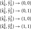
Specifically, transcritical bifurcations can occur (i.e., one equilibrium overlaps with another, and they exchange their stability), when the interior equilibria collapse with the corner equilibria, that is, when $W_{1}=W_{2}=\frac{2\beta +\sigma }{b},$ in which the trivial and nontrivial equilibria collide. For example, poverty-trap regimes must disappear when a bifurcation occurs (see Figure 3), which implies that the four interior equilibria collapse with the four nearest corner equilibria. Thus, each of the interior equilibria, $((\hat{\mathrm{x}}_{\mathrm{E}}^{1},\hat{\mathrm{y}}_{\mathrm{E}}^{1}), (\hat{\mathrm{x}}_{\mathrm{E}}^{2},\hat{\mathrm{y}}_{\mathrm{E}}^{2}), (\hat{\mathrm{x}}_{\mathrm{E}}^{3},\hat{\mathrm{y}}_{\mathrm{E}}^{3}),\text{ and }(\hat{\mathrm{x}}_{\mathrm{E}}^{4},\hat{\mathrm{y}}_{\mathrm{E}}^{4}))$ , collides (shifting and wrapping) at the nearest corner equilibrium $((0,0), (0,1), (1,0), (1,1))$ , namely:

\begin{align*}& (\hat{\mathrm{x}}_{\mathrm{E}}^{1},\hat{\mathrm{y}}_{\mathrm{E}}^{1})\rightarrow (0,0)\\& (\hat{\mathrm{x}}_{\mathrm{E}}^{2},\hat{\mathrm{y}}_{\mathrm{E}}^{2})\rightarrow (0,1)\\& (\hat{\mathrm{x}}_{\mathrm{E}}^{3},\hat{\mathrm{y}}_{\mathrm{E}}^{3})\rightarrow (1,0)\\& (\hat{\mathrm{x}}_{\mathrm{E}}^{4},\hat{\mathrm{y}}_{\mathrm{E}}^{4})\rightarrow (1,1)\end{align*}

This happens when $W_{1}=W_{2}\geq \frac{2\beta +\sigma }{b}$ , which means that the per-capita income must be greater than the cost of education determined by the conditions of the labor market and peer effects, and this declines as skill premiums rise. Therefore, to obtain the high-level equilibrium, per-capita income must grow and, thus, incomplete education must decrease.

Considering this evolutionary game, we get the cases of a multiplicity of equilibria or poverty-trap regimes. Poverty-trap regimes exist with different levels of poverty characterized by various levels of complete and incomplete education and per-capita income. We now analyze empirically, with inferential statistics, the poverty of agents in Mexican municipalities as players in the game of poverty in Mexico. We do not estimate the strategies that agents choose but rather the effects of incomplete education and per-capita income. In doing so, we analyze the dynamics and formation of poverty-level regimes in Mexico. To this end, we apply symbolic dynamic techniques that result in equilibria/stable poverty regimes (e.g., moderate poverty or high poverty).

3. Dataset and methodology

The first goal of this section is to describe the dataset that will be used for the statistical inference analysis; the data include the poverty rate, incomplete education, and per-capita income for Mexican municipalities. The second goal is to describe and apply the statistical methodology approach to study the regimes that give the relationship between education and poverty.

The dataset includes three main variables for N = 2430 municipalities in 2000, 2005, 2010, 2015, and 2020 (T = 5). Thus, we are working with 5-year data and a subset of the 2469 municipalities for which information is available for the entire period. Particularly:

• The poverty rate ( P ) of a municipalityFootnote ¹⁵ is obtained from the multidimensional poverty rate starting in 2010 and is properly combined with a variation of the income poverty (heritage) to obtain P for 2000 and 2005.

• The percentage of the population aged 15 years or older with basic incomplete education ( IE ) is also obtained from CONEVAL, and the variable is part of the Social Gap Index (IRS).Footnote ¹⁶

• The per-capita income ( YL ) is a control variable proxied by the corresponding Mexican state’s per-capita GDP at 2013 constant values, which is obtained by dividing the state’s GDP by the state’s population. It is taken from the National Institute of Geography and Statistics (INEGI).Footnote ¹⁷

Then to study the Mexican poverty regime dynamics, we applied two complementary methodologies: symbolic regimes with symbolic time series and econometric panel data.

3.1. Data symbolization and regimes

Municipality poverty in Mexico is studied by identifying different regimes of poverty. To identify these and their dynamics, symbolic analysis is applied. The concept of symbolization has its roots in dynamical systems theory, particularly in the study of nonlinear systems, which can exhibit bifurcation and chaos. Williams (Reference Williams2004) asserts that symbolic dynamics is a method for studying nonlinear discrete-time systems by taking a previously codified trajectory using strings of symbols from a finite set, also called an alphabet. According to Piccardi (Reference Piccardi2004), symbolic dynamics and symbolic analysis are connected but different concepts. The former is the practice of modeling a dynamical system using a discrete space. However, the latter is an empirical approach to characterizing highly noisy data by considering a partition, discretizing the data, and obtaining a string representing the very dynamic of the process. For a discussion of symbolization and symbolic time series, see Risso (Reference Risso2018), Piccardi (Reference Piccardi2004), Hirata et al. (Reference Hirata, Judd and Kilminster2004), Daw et al. (Reference Daw, Finney and Tracy2003), Kurths et al. (Reference Kurths, Schwarz, Witt, Krampe and Abel1996), and Bollt et al. (Reference Bollt, Stanford, Lai and Życzkowski2001).

In practice, symbolization is applied by defining equally probable regimes in time series. With our three variables (poverty rate, incomplete education, and per-capita GDP), the following four regimes are defined:

1. 1. = { x : x $\leq$ μ_x25%} (low regime)

2. 2. = { x : x $\leq$ μ_x50% and x $\gt$ μ_x25% } (medium regime)

3. 3. = { x : x $\leq$ μ_x75% and x $\gt$ μ_x50%} (high regime)

4. 4. = { x : x $\gt$ μ_x75%} (very high regime)

where μ_x25%, μ_x50%, and μ_x75% are the corresponding percentiles of x at 25%, 50%, and 75%, respectively. Considering the 25th, 50th, and 75th percentiles as limits, four poverty regions are defined in Mexico, given by the following four symbols (1,2,3,4):

1. 1. Low poverty (p $\leq$ 52%),

2. 2. Medium poverty (52% $\lt$ p $\leq$ 69%),

3. 3. Medium-high poverty (69% $\lt$ p $\leq$ 84%),

4. 4. High poverty (p $\gt$ 84%),

where p is the municipal poverty rate.

Four regimes were chosen for two reasons. First, it is a manageable number of regimes to study the dynamic: two symbols would be a simple binary variable (low, high), and more than four would complicate the sequential analysis (e.g., analyzing patterns of three periods implies eight possible cases, four implies 64 cases, and five implies 125 cases) and reduce robustness in a sample of 2430 municipalities and five different years. Second, there are four equilibria in the theoretical model, and we want to allow the possibility of obtaining the four equilibria in the different regimes.

This symbolization will enable us to study the temporal transition from one regime to another or permanence in one regime, that is, the multiple-equilibria transition. For example, in a given municipality, temporal sequences of three periods of poverty could be (1,1,1), (4,4,4), (1,2,3), and so on. If the dynamics are independent, all the sequences should have the same probability. We test independence using the symbolic independence test proposed by Risso (Reference Risso2014) and Monte Carlo simulations. In addition, we can study a type of symbolic dependence of poverty (p) on per-capita GDP (YL) and incomplete education (IE) by analyzing symbolic sequences such as (IE(t−1), YL(t−1), p(t)) using the symbolic causality test proposed by Risso (Reference Risso2015), where previous determinant variables (IE and YL) affect the present poverty rate.

3.1.1. Symbolic dynamics for Mexican municipalities

Considering the model described in Section 2 and the symbolic methodology, we empirically analyze the distribution of the players’ profiles (i.e., the Mexican municipalities). The map in Figure 4 shows the distribution of poverty regimes in Mexican municipalities in 2020. As can be seen, the low- (or lower-) poverty regimes are concentrated in the north of the country and on the northwest coast, whereas higher-poverty regimes are found in the south.

Figure 4.

Municipal poverty in 2020. Source: own elaboration.

Figure 5 shows the percentage of municipalities that are in temporal sequences of three 5-year periods between 2000 and 2020. Being 3 symbols the combinations of 3, we find 64 different dynamics of (p(t−2), p(t−1), p(t)). One of the first observations is the high persistence of municipalities in regions: 51.1% of the municipalities have remained in the same region for three 5-year periods between 2000 and 2020. More precisely, 16.6% have remained in the low-poverty region (1, 1, 1) = (111), 9.5% in the medium-poverty region (2, 2, 2) = (222), 8.6% in the medium-high-poverty region (3, 3, 3) = (333), and 16.4% in the high-poverty region (4, 4, 4) = (444). This empirical evidence indicates that a stable low-level equilibrium may be verified in the Mexican case, that is, a steady state of stable poverty in Mexico.

Figure 5.

Poverty sequence frequencies {p(t−2), p(t−1), p(t)}. Source: own elaboration.

Conversely, some municipalities have gone from high levels of poverty to lower levels, namely (211), (221), (231), (241), (311), (312), (321), (322), (331), (332), (341), (342), (411), (412), (413), (421), (422), (423), (431 ), (432), (433), (441), (442), and (443), representing 25.8% together. This gives rise to multiple steady-state equilibria for the Mexican case. Moreover, emphasizing the multiple equilibria and, in particular, the stability toward the low-level equilibrium (the poverty trap), Figure 5 also shows that 11.1% of the municipalities have moved from low to higher levels of poverty: 112, 113, 114, 122, 123, 124, 132, 133, 134, 142, 143, 144, 213, 214, 223, 224, 233, 234, 243, 244, 314, 324, and 334. The remaining 12.2% represent oscillating sequences since they started and ended in the same region. This multiplicity of equilibria as a distribution of sequences is not random; we run 10,000 Monte Carlo simulations of the same sample size, and the distribution would be like the red dotted line if it were random.

In addition, an independence test for symbolic series is performed as in Risso (Reference Risso2014). The test considers a finite time series generated by an independent or random process sized T. We define a partition in the series in “a” equiprobable regions, obtaining the symbolized time series {s_t }. Each symbolized variable s_t takes a symbol value from the alphabet A = {A ₁, A ₂, … A_a}. We can define a rolling window w over the symbolized time series T, and we obtain n = a^w possible events. S_i being the sum of each possible event for i = 1, 2, …, n, since the series is random, each S_i should have the same probability or S_i /T = 1/n. For simplicity, we imagine a time series from a dice A = {1,2,3,4,5,6} and a rolling window of 3 should define n = 6³ = 216 possible events (where 1,5,3 is a possible event), and, due to randomness, each S_i /T should have a probability of 1/6. Because the time series is finite and sized T, a statistic is needed. Each error ((S_i/T) − (1/n)) in a finite random process should be near 0 and is multivariate normal distributed for each i. Finally, considering the distribution of quadratic normal variables explained by Mathai and Provost (Reference Mathai and Provost1992), we can consider the statistic $Tn\{\sum((S_i/T)-(1/n))^2\}$ asymptotically distributed as a Chi-squared with n−1 degree of freedom.

Applying the independence test for symbolic series, we obtain a statistic of 9119.86 which, compared with a Chi-squared of 63 degrees of freedom at 95%, 82.53 rejects the hypothesis that the sequence is random. In addition, the mean of the simulations gives a statistic of 0.01, well below the critical value, indicating a random sequence.

The map in Figure 6 shows that between 2010 and 2020, most municipalities remained in the same poverty regime (gray). However, a large number of municipalities concentrated in the center of the country descended toward lower poverty regimes. Among those that increased, for example, the Felipe Carrillo Puerto municipality in Quintana Roo stands out: despite having reduced the levels of incomplete education (as a proxy for illiteracy) and being characterized by high average income levels, it has not been able to overcome the issue of poverty, which has instead worsened.

Figure 6.

Variation of poverty in municipalities (2010–2020). Source: own elaboration.

With the above, we have shown the multiplicity of equilibria and the diversity of poverty (high, medium, and low) existing in Mexico. We now consider what was shown by the evolutionary game model described above, which revealed the primary role of the cost of education (educational backwardness) and per-capita income (wages, prices, and bonuses). Hence, we analyze the role of incomplete education and income.

3.1.2. The role of incomplete education and income (GDP per capita)

Other deficiencies that increased, albeit to a lesser extent, are the educational gap (0.25 percentage points) and the lack of access to nutritious and quality food (0.31 percentage points). Figure 7 shows the municipal histogram of the percentage of the population aged 15 years or older with incomplete basic education in 2000, 2010, and 2020. The movement to the left from 2000 to 2020 is clearer than in the case of the poverty rate, indicating a general reduction of this indicator. The average rate of incomplete education was 72.3% in 2000 and 45.7% in 2020, and the percentage of municipalities with a rate of incomplete education of 70% or above decreased from 63% in 2000 to 4% in 2020. At the same time, the percentage of municipalities with 30% of incomplete education or less increased from 0% to 15% in the same period. Low levels of incomplete education are concentrated in the north of the country and part of the Yucatan peninsula.

Figure 7.

Distribution of incomplete education in the municipalities. Source: own elaboration.

In the following, we characterize once again the multiple equilibria (steady states) for the Mexican municipalities. We consider data for the following variables: (i) incomplete education rate (E), (ii) GDP per capita of the federal state in which the municipality is located (Y), and (iii) poverty rate of the municipality (P). Four regions were defined for each variable:

1. 1. Low (below the 25% percentile)

2. 2. Medium (between 25% and 50%)

3. 3. Medium-high (between 50% and 75%)

4. 4. High (above the 75% percentile).

We thus obtain the following characterizations:

• E1 (low incomplete-education rate), E2 (medium incomplete-education rate), E3 (medium-high incomplete-education rate), E4 (high incomplete-education rate).

• Y1 (low income), Y2 (middle income), Y3 (upper middle income), Y4 (high income).

• P1 (low-poverty rate), P2 (medium-poverty rate), P3 (medium-high poverty rate), P4 (high-poverty rate).

With this symbolization of the variables, the causality sequence of predetermination (E(t−1), Y(t−1), P(t)) is analyzed. It shows how a municipality is affected by being in a region of poverty at time t when it was in a region with a given incomplete-education rate and per-capita income at time t−1.

Table 2 shows that some frequencies are much higher than the frequency that would be found if the sequences were random (i.e., 1.56%). For example, the sequence (414) has a 10.4% appearance. That is, if one was in a region of very high incomplete education (E4) and low income (Y1) in period t−1, one will be at a very high-poverty level (P4). Likewise, the sequence (141) has a probability of 6.9%, which means that if one is in a region with low incomplete education (E1) and a very high-income level (Y4), at time t, one is at a low-poverty level (P1). We perform 10,000 Monte Carlo simulations for this process and find that this sequence is far from independent and, therefore, significant. The causality test for symbolic series [Risso (Reference Risso2015)] indicates that it is significant with a statistic of 9119.86 and a Chi-squared (63) at 95% of 82.53, so the hypothesis of no causality. The statistic for the mean of the simulations is 0.01, well below the critical value mentioned above.

Table 2.

Sequences of E(t−1), Y(t−1), P(t), and the frequency in municipalities

Source: Own elaboration.

From Table 2, the figures below are obtained, which show the evolution of the probability of being at low levels of poverty at time t for increasing regimes of incomplete education (Figure 8a) and the same probability given increasing regimes of per-capita GDP (Figure 8b). We observe that if at t−1, a municipality was in a low incomplete-education level (E1) and high-income region (Y4), the probability of being in the low-poverty region P1(t) at t is 90%. Conversely, if a municipality is at higher levels of incomplete education at t−1, even if it is at a high-income level (Y4), the probability that it will be in the low-poverty region decreases to 64% if the municipality is in incomplete education E2, to 45% if it is in the E3 region, and to 36% if it is in the E4 region. Hence, this shows the importance of reducing the values of incomplete education (illiteracy or educational backwardness) since even being in regions of higher average income at time t−1, there is only a 36% probability of being in the low-poverty region P1.

Figure 8.

(a) Probability of low poverty (P1) given increasing level of incomplete education (E). (b) Probability of low poverty (P1) given increasing level of per capita GDP (Y). Source: own elaboration.

Figure 8b reveals a growing probability of low poverty as the per-capita GDP increases. However, for a low level of incomplete education E1, given Y1, the probability of P1 is 62%, and for a low incomplete education E1, given Y2, the probability of P1 is 57%. With a low level of incomplete education E1, we have to reach the very high regime of income (Y4) to observe a probability of 90% of being in a low-poverty regime P1.

Maps (Figure 9a and b) show that between 2010 and 2020, the geographical areas with the lowest rate of incomplete education shrunk. In particular, more green areas are seen in the north of the country and part of the Yucatan peninsula.

Figure 9.

(a) Mexico: incomplete education in 2010. (b) Mexico: incomplete education in 2020. Source: own elaboration.

Regarding income (Figure 10a and b), it can be noticed that the highest is also found in the north of the country and that in 2020, the places with the highest income expanded, together with the Yucatan peninsula.

3.2. Econometric results

To complement the results obtained by the symbolic analysis, we first perform a panel data causality test. Then, we use random effect (RE) panel data as shown in equation (2), as suggested by Bell and Jones (Reference Bell and Jones2015), who remarked that RE can provide everything that fixed effects promises and more. As a second model, we consider the Arellano–Bover/Blundell–Bond method proposed by Arellano and Bover (Reference Arellano and Bover1995) and Blundell and Bond (Reference Blundell and Bond1998), as expressed in equation (3).

(2) \begin{equation}\text{Ln}(p)_{i,t} = \alpha_{1}+\alpha_{2}\text{Ln(EI)}_{i,t}+\alpha_{3}\text{Ln(YL)}_{i,t}+\upsilon_{I} \end{equation}

(3) \begin{equation}\Delta(\text{Ln}(p))_{i,t}=\beta_1\Delta(\text{Ln}(p))_{i,t-1}+\beta_{2}\Delta(\text{Ln(EI)})_{i,t}+\beta_3\Delta(\text{Ln(YL)})_{i,t}+\Delta\epsilon_{i,t} \end{equation}

where Ln(p) _{i , t} , Ln(IE) _{i , t} , and Ln(YL) _{i , t,} respectively, define the logarithm of poverty, incomplete education, and per capita GDP with municipality I = 1, 2, …, n and year t = 2000, 2005, 2010, 2015, 2020, and the variables in the second model are in differences, that is, D(Ln(p)) _{i , t− 1} = Ln(p) _{i , t} − Ln(p) _{i , t− 1}.

In the present analysis, the determinants of the poverty rate of the municipalities of Mexico are evaluated using panel data (N = 2430 and T = 5, with 12,150 observations). The variables are the poverty rate of the municipalities of Mexico, the rate of incomplete education (educational backwardness, illiteracy) in the municipalities of Mexico, and the GDP per capita (income) of the federal states to which the municipalities belong.

Table 3 shows the results of the Granger causality test for panels. We observe that both the share of the population with incomplete education and the GDP per capita of the federal state to which the municipality belongs cause the poverty rate in the sense of Granger (i.e., they currently predict it).

Table 3.

Panel VAR-Granger causality Wald test

Source: Own elaboration. *rejection of the null hypothesis at 0.01.

Figure 10.

(a) Mexico: per-capita income in 2010. (b) Mexico: per capita income in 2020. Source: own elaboration.

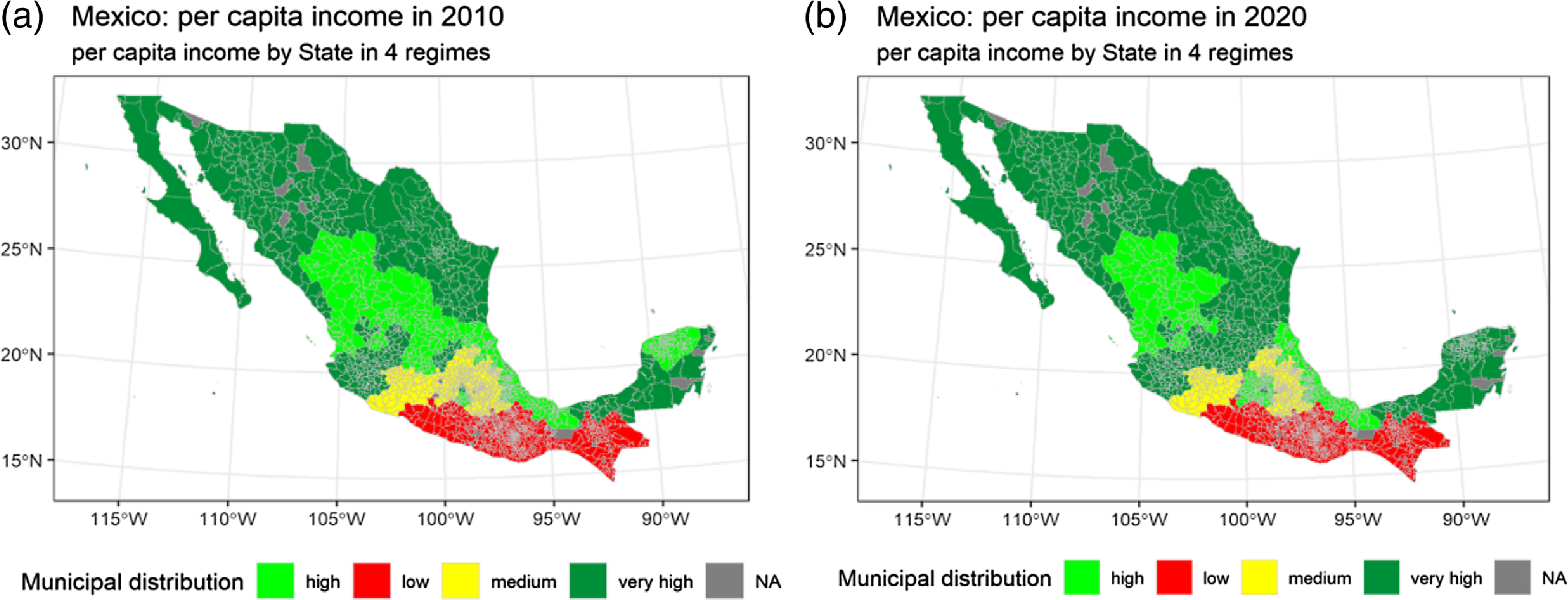
Table 4 presents the results of the RE and Arrellano–Bover/Blundell–Bond models. The coefficients are statistically significant, with the expected signs. That is, the incomplete education rate has an elasticity between 0.23 and 0.34, which means that an increase of 100% in the rate of incomplete education results in a 23% increase in the poverty rate. The long-run elasticity is 0.28.

Table 4.

Econometric model results

Source: Own elaboration. *significance at 0.1, **significance at 0.05, and ^***significance at 0.01.

The GDP per capita of the state also harms the poverty rate. As can be seen, in the Arellano Bond model, the short-term elasticity is −0.44, and the long-term elasticity is 0.55. Thus, an increase of 100% in the GDP per capita reduces the poverty rate by 55%. In addition, the COVID-19 pandemic worsened poverty, with a long-run elasticity of 0.03.

3.2.1. Time elasticities

To study the evolutionary dynamics of the elasticities of incomplete education and income over the poverty rate, a cross-section model is applied for each year, and the changes over the years are examined.

Table 5 shows that the elasticity of incomplete education fell from 1.02 in 2000 to 0.56 in 2020, indicating a decrease in the impact of this variable on poverty reduction. This means that reducing incomplete education still reduces poverty but less strongly, and increasing incomplete education increases poverty but less strongly.

Table 5.

Elasticity of incomplete education and per capita GDP on poverty

Source: Own elaboration. *significance at 0.01.

In the case of state GDP per capita, there is an increase (in absolute value) in its impact on poverty from −0.38 in 2000 to −0.46 in 2015. That is, increasing per-capita income is constantly positive in the magnitude of its impact on the reduction of poverty. Nevertheless, it can also be seen that between 2015 and 2020, the elasticity of income remained constant. In short, the goals of improving the levels of education and increasing the income of Mexicans have not been ambitious enough to escape the Mexican poverty traps. It is time to act more harshly, steadily, and lastingly to increase the levels of quality education together with income for all Mexicans, with a view to overcoming the poverty traps.

We also performed Arellano–Bover/Blundell–Bond modeling in a 4-year window to check for the evolution of the elasticities. The results are summarized in the following table, which reveals that, according to the model, the impact of incomplete education has increased from 0.10 to 0.18 between 2000–2015 and 2005–2020. Likewise, the impact of GDP per capita rose from 0.19 to 0.33 in the same period.

The implication of the growing impact of incomplete education in the last 15 years is that education levels in Mexico have not risen at all, quite the opposite; therefore, poverty continues to be present as a stable and stationary state. Thus, in the last 15 years, increases in income have been key but insufficient to get out of the poverty traps. In other words, as previously stated, better levels of education and higher levels of income are sustained and lasting and are the key to overcoming poverty traps.

4. The “big push” policy

Considering the estimated econometric model, we project scenarios to analyze the evolution of poverty regimes, which are overcome according to possible variations in per-capita income and the rate of incomplete education.

Per-capita income increased on average by 9% in 2010–2015 and decreased by 9% in 2015–2020, while incomplete education fell on average by 12% in 2010–2015 and by 14% in 2015–2020. Therefore, the first scenario assumes that the per-capita income remains the same (0%) in 2020–2025 and 2025–2030, with a decrease of 15% in incomplete education in each quinquennial (2020–2025 and 2025–2030). Table 7 presents the results of this scenario and others. In scenario 1, the percentage of municipalities in regime P4 (very high poverty) would be 0.9% in 2025 and 0.2% in 2030, and most of the municipalities fall under regime 1 (low poverty), going from 33.5% in 2020 to a projected 51.8% in 2030. This is an important result; however, it should be noted that the Mexican low-poverty regime corresponds to a poverty rate of 51.43% or lower, which remains high in the international context.

Table 6.

Elasticities of incomplete education and per capita GDP considering two temporal windows and the Arellano–Bover/Blundell–Bond

Source: Own elaboration. **significance at 0.05 and ^***significance at 0.01.

Table 7.

Distribution of municipalities by poverty regimes for different scenarios

Source: Own elaboration.

The results of the scenarios indicate that for 0% of the municipalities to be in poverty regime 4 (high poverty, in which more than 84% of the citizens are poor) in 2030, a 10% decrease is necessary during the two 5-year periods 2020–2025 and 2025–2030 as well as a 10% increase in per-capita income in the same periods. This means that between 2020 and 2025, each municipality should lower its rate of incomplete education by 10% and increase its per-capita income by 10%, and then again between 2025 and 2030.

Therefore, as shown by the evolutionary game of poverty traps developed above, the income/wages (or marginal income) obtained when the levels of education are completed, bW_i, are so high that they cover the costs of education and any negative effects or synergies between peers facing citizens with an incomplete education. Therefore, completing education is economically profitable, which makes the economy fully converge toward complete-education status for its high per-capita income citizens. Thus, poverty-trap regimes are repulsive, with the high equilibrium being the unique asymptotically stable equilibrium.