1. Introduction
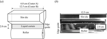
Curtain coating is a technique used for depositing a liquid curtain on a moving solid surface (substrate) (see Kistler Reference Kistler1985; Miyamoto & Katagiri Reference Miyamoto and Katagiri1997; Weinstein & Ruschak Reference Weinstein and Ruschak2004). The liquid curtain in curtain coating is produced by flowing the liquid discharged from the gap of the slot die to the edge guides on the left and right ends, the substrate, moving at a constant speed, is placed at the lower end of the liquid curtain and the liquid curtain is deposited on the substrate (see figure 1, where the substrate has been removed from the roller). When the speed of the moving substrate increases, air gets entrained to the liquid film on the substrate or the liquid-curtain break-up occurs from the edge guide. Hence, the prediction method of the liquid-curtain behaviour is a subject of research (for instance, Blake & Ruschak Reference Blake and Ruschak1979; Liu et al. Reference Liu, Vandre, Carvalho and Kumar2016; Liu, Carvalho & & Kumar Reference Liu, Carvalho and Kumar2019). In this study, we report the propagation of the rim of the liquid curtain due to the liquid-curtain breakup.
Liquid curtain formed in the area surrounded by slot die, edge guide and roller. (a) Schematic view of experimental device. (b) Front view of slot die, liquid curtain and roller. Coater A: 6.0 cm wide slot and 0.3 mm wide slit. Coater B: 12.5 cm wide slot and 0.1 mm wide slit. (b) shows the photograph of Coater B.

The liquid-curtain volume flow rated from the slot die can be bridged to the edge guides, and the liquid is transferred to the roller surface as shown in figure 1 (for instance, Takagi Reference Takagi2010; Kyotoh et al. Reference Kyotoh, Fujita, Nakano and Tsuda2014; Liu, Itoh & Kyotoh Reference Liu, Itoh and Kyotoh2017). However, in the vicinity of the contact between the edge guide and roller, the liquid curtain becomes thinner and the mechanical vibrations of the roller influence the stability; hence, the liquid curtain may become unstable and break up at the contact. The small hole at the beginning of the breakup grows in the direction of the liquid curtain, a rim develops by absorbing the liquid and, finally, the liquid curtain disappears between the edge guides. In this study, the propagation speed, shape and stability of the rim are observed experimentally and evaluated using a theory to understand how to prevent the rupture of the liquid curtain by investigating the factors governing the rim propagation.
The breakup of the liquid curtain was studied by Taylor and Culick, who expressed its propagation speed as  $c_s\equiv \sqrt {2\sigma /(\rho \, H)}$, where
 $\rho$: liquid density,
 $H$: liquid-curtain thickness,
 $\sigma$: surface tension (see Taylor Reference Taylor1959; Culick Reference Culick1960). The liquid pool at the breakup boundary is referred to as the rim, and its mass increases by absorbing the liquid in the curtain as it propagates; however, its propagation speed is nearly constant. The effect of the liquid viscosity on the rim shape and propagation speed has been discussed (see Brenner & Gueyffier Reference Brenner and Gueyffier1999; Sunderhauf, Raszillier & Durst Reference Sunderhauf, Raszillier and Durst2002; Savva & Bush Reference Savva and Bush2009); capillary waves appear behind the rim for small Ohnesorge numbers, the rim disappears for large Ohnesorge numbers and the viscosity has no influence on the propagation speed.
Entov & Yarin (Reference Entov and Yarin1984) derived the equation of motion of the liquid-curtain rim considering viscosity and surface tension (see also Yarin Reference Yarin1993). This equation describes the motion of the fluid particles at the centreline of the rim in the Lagrangian coordinate system and can be applied to the rim with an arbitrary shape in space; however, the cross-section of the rim is circular and the flow velocity inside it is assumed to be uniform. The condition in which the rim has a circular cross-section is valid for the liquid curtain with an Ohnesorge number roughly less than 1 (see Sunderhauf et al. Reference Sunderhauf, Raszillier and Durst2002). Moreover, based on this equation, the stability of the line rim, whose radius and flow velocity are a function of time, is expressed through a variable coefficient ordinary differential equation (Roisman Reference Roisman2010; Agbaglah, Josserand & Zaleski Reference Agbaglah, Josserand and Zaleski2013). They show that the instability can be studied by determining the eigenvalues obtained under the assumption that the variable coefficients of the disturbance equation are constant, i.e. frozen rim or frozen parameter, and discussed the effects of liquid viscosity and surface tension on rim stability. Roisman (Reference Roisman2010) specifically calculated the moment of moment equation and showed that the shear force in the rim cross-section has a small effect on the stability of the rim. In contrast, curtain coating requires analysis that takes gravity into consideration because liquid in a curtain coating is transferred to the substrate by utilising the inertial force of gravity.
In curtain coating, when the Weber number defined by  $We\equiv (U/c_s)^{2}$ (
 $U$ being the flow velocity in the liquid curtain) was greater than 1, the equation of motion of the rim associated with the breakup of the liquid curtain was derived, and the rim shape for the steady state case was obtained (Roche & Le Grand Reference Roche and Le Grand2006). When the Weber number is smaller than 1, the propagation speed of the rim exceeds the flow velocity in the liquid curtain, causing the liquid curtain to disappear between the edge guides. However, it has been experimentally shown that the viscosity of the liquid and the inertia of the rim enlarge the coatable area in the coating window, and that the liquid curtain is stable even when the Weber number is less than 1 (see Roche & Le Grand Reference Roche and Le Grand2006; Marston et al. Reference Marston, Thoroddsen, Thompson, Blyth, Henry and Uddin2014; Karim, Suszynshi & Francis Reference Karim, Suszynshi and Francis2018). Furthermore, in curtain coating, the liquid curtain is surrounded by slot die, edge guides and a roller, which also affect stability of the liquid curtain, for example, the viscous boundary layer on the edge guides causes instability (Karim et al. Reference Karim, Suszynshi and Francis2018), and the high viscous liquid curtain bridged between parallel needles suppresses the rim growth (Chepushtanova & Kliakhandler Igor Reference Chepushtanova and Kliakhandler Igor2007).
In this study, the liquid-curtain breakup and rim propagation are studied experimentally and theoretically. Here, the shear force considered by Entov & Yarin (Reference Entov and Yarin1984) and Roisman (Reference Roisman2010) is ignored, but the gravitational force is considered because it is crucial for curtain coating. In § 2, experiments are performed to observe the breakup of the liquid curtain bridged by the rotating roller, and the shape and propagation speed of the rim are measured. In § 3, the equation of motion of the rim is analysed, and the shape and propagation speed of the rim of the liquid curtain are obtained and compared with the experimental values. In § 4, the stability of the rim is theoretically evaluated and the separation of the droplets from the rim is discussed from the linear stability analysis. Finally, in § 5, we discuss the shape, propagation speed, the stability of the rim and show the importance of the gravitational force on the liquid-curtain rim.
2. Breakup of liquid curtain bridged to rotating roller
To examine the possibility of curtain coating at a low flow rate, that is, at a low Weber number, a liquid curtain is disrupted by a stainless rod to cause the liquid curtain breakup at the contact of the edge guide and roller, and this is photographed using a high-speed video camera. The image is then analysed to measure the rim shape and propagation speed. The experiment was performed using two types of slot dies (Coater A: slit width 0.3 mm, slot width 6.0 cm, Coater B: slit width 0.1 mm, slot width 12.5 cm). In both cases, the drop height of the liquid curtain is 2.0 cm.
In the experiment with Coater A, a high-viscosity liquid was used as the working fluid, and the droplets did not break away from the rim. In the experiment with Coater B, a low-viscosity liquid was used, the Ohnesorge number was small and the droplets broke away from the rim.
2.1. Experimental set-up and method
In the experimental set-up shown in figure 1, a liquid curtain is generated by discharging liquid from a slot die, bridging between the left and right edge guides and transferring the liquid to a rotating roller. In the experiment, two different coating dies are installed, i.e. Coater A with a width of  $6.0\ {\rm {cm}}$ and a slit width of
 $300\ \mathrm {\mu }{\rm m}$ and Coater B with a width of
 $12.5\ {\rm {cm}}$ and a slit width of
 $100\ \mathrm {\mu }{\rm m}$, but the falling height of the liquid curtain is fixed at 2.0 cm. The working liquid is circulated by a diaphragm pump (Tacmina TPL2M-028). A high-speed video camera (Photron Fastcam SA4) is installed to photograph the liquid curtain from the front, and the video image is analysed during the curtain breakup to measure the rim propagation speed and shape.
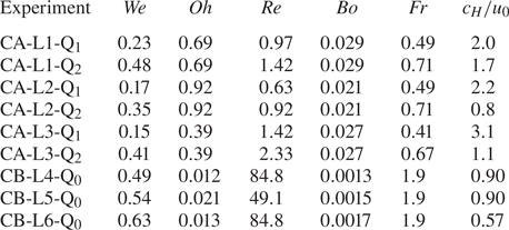
The working liquid used in this experiment is a mixture of water, glycerin and ethanol. The viscosity of the liquid  $\mu$ and the surface tension
 $\sigma$, vary according to the mixing ratio of the liquids (see table 1). This liquid is a Newtonian fluid, and the dimensionless dominant parameters describing the physical properties are the Weber number, Ohnesorge number, Reynolds number, Bond number and Froude number defined by
 \begin{align} We=\frac{\rho H_0 {u_0}^{2}}{2\sigma}, \quad Oh=\frac{\mu}{\sqrt{\rho\sigma H_0}}, \quad Re=\frac{\rho u_0 H_0}{\mu}, \quad Bo=\frac{\rho g {H_0}^{2}}{\sigma}, \quad Fr=\frac{u_0}{\sqrt{g h}}, \end{align}
where  $\rho$ is the density, g is the gravitational acceleration,
 $H_0$ and
 $u_0$ are the liquid-curtain thickness and flow velocity at the slot die exit,
 $h$ is the distance from the slot die exit to the top of the roller and
 ${We}$ is the value at the slot die exit. It should be noted that we use half the liquid-curtain thickness as the length scale of the Weber number. We conducted experiments on the six cases for Coater A and three cases for Coater B as presented in table 2.
Liquid properties. W: water, G: glycerin, E: ethanol.

Experimental conditions.

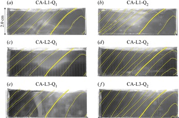
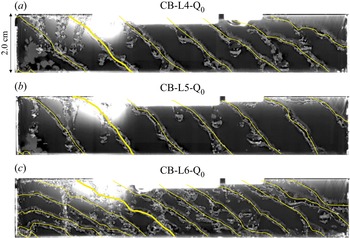
The rightmost column in the table is the horizontal propagation speed  $c_H$ of the rim described by the bold yellow curve shown in figures 2 and 3. Also, CA and CB show the experiment by Coater A and Coater B, respectively, and
 ${\rm L1}\unicode{x2013} {\rm L6}$ denotes Liquid
 $1\unicode{x2013} {\rm Liquid}\ 6$ in table 1, respectively.
Front image of the rim propagation (supplementary Movie A available at https://doi.org/10.1017/jfm.2022.547). An image from the high-speed video camera depicting the liquid curtain in the area surrounded by the left and right edge guides, slot die exit and roller is shown superimposed every 12/500 s. The breakup occurs from the contact point between the right edge guide and the roller. The yellow line in the figure depicts the centreline of the rim, and the CA in the title indicates that the experiment was performed using Coater A. Additionally, L and Q in the title indicate the working liquid and flow rate, respectively (see table 1).

Front image of the rim propagation (supplementary Movie B). An image of the high-speed video camera depicting the liquid curtain in the area surrounded by the left and right edge guides, slot die exit and roller is shown, superimposed every 12/500 s. The breakup occurs from the contact point between the left edge guide and the roller. The yellow line in the figure depicts the centreline of the rim, and CB in the title indicates that the experiment was performed using Coater B. In addition, L and Q in the title indicate the working liquid and flow rate, respectively (see table 1).

CA and CB in table 2 represent Coater A and Coater B,  ${\rm L1}\unicode{x2013} {\rm L6}$ are the liquids listed in the table 1 and
 ${\rm Q}_{0}$,
 ${\rm Q}_{1}$,
 ${\rm Q}_{2}$ are volume flow rate listed in the table 1, for example CA-
 ${\rm L1}$-
 ${\rm Q}_{1}$ is the experiment with Coater A, liquid
 ${\rm L1}$, and volume flow rate
 ${\rm Q}_{1}$. From table 2, the viscous stress of the liquid curtain is of the same order as the surface tension in experiment CA, and the surface tension is dominant over the viscous stress in experiment CB. In experiment CA, the liquid curtain coming out of the die accelerates, the thickness decreases to approximately 0.5 times the slit width at the lower end of the liquid curtain and the Weber number becomes close to 1.
The rotation speed of the roller is adjusted so that the liquid flow velocity reaching the roller surface is almost the same as the roller peripheral speed. The Weber number in table 2 is the value at the slot die exit, which then increases downstream. Conversely, the Reynolds number does not change on the liquid curtain.
2.2. Experimental results
In experiment CA, the breakup of the liquid curtain is caused by disrupting the lower right end of the curtain using a stainless steel rod. In experiment CB, the liquid curtain broke from the contact point between the left edge guide and roller. Because the Weber number used in this paper is smaller than 1, the breakup propagates throughout the liquid curtain. In the Coater A experiment, there was no detachment of droplets from the rim. Conversely, in the Coater B experiment, the droplets detached from the rim during the propagation. The results of these experiments are presented separately below.
2.2.1. Coater A experiment: detachment of droplets from the rim
A rim was generated from the lower right corner in figure 2. The liquid curtain was photographed from the front at 500 f.p.s. by the high-speed video camera, and the shape and surface of the rim were visualised by superimposing the rim images every 12/500 s. The yellow line in figure 2 traces the centreline of the rim, and the diameter of the rim can be observed when the electronic images of figure 2 are enlarged.
The rim acquires the liquid in the curtain and propagates vertically upward while growing. Subsequently, the upper end of the rim reaches the slot die exit and propagates toward the leftmost edge guide. Further, after the top of the rim reaches the slot die exit, the liquid in the rim flows vertically downward along the rim (see supplementary Movie A). Similar experiments were performed four times for each experimental case, but no significant difference was observed in the rim shape.
The Weber numbers in the right and left columns in figure 2 are approximately 0.2 and 0.4, respectively. The propagation speed of the rim, represented by the bold yellow line, is depicted in the last column of table 2. This value is roughly the same as that calculated from (3.21a,b), derived later in § 3.2.2. In figure 2(a,c,e), the rim centreline is convex downward and the centreline spacing is narrow, because the liquid lump on the rim flows down and the horizontal propagation speed of the rim decreases.
2.2.2. Coater B experiment: detachment of droplets from the rim
The slit width of Coater B is 0.1 mm and the pressure loss is high. Therefore, a low-viscosity liquid was used as the working fluid. Consequently,  $Re$ is approximately 80 and
 $Oh$ is approximately 0.01, that is, the influence of viscosity on the flow is much smaller than that of the surface tension.
The liquid curtain was photographed from the front at 5000 f.p.s. by a high-speed video camera, and the shape and surface of the rim were visualised by superimposing the images every 12/500 s. The yellow line in figure 3 traces the centre of the rim, and the diameter of the rim can be determined from these images. Compared with the experimental results of Coater A, the surface of the rim is not smooth in this experiment; a liquid lump is formed on the rim, and the droplets are separated from the rim. In figure 3, three types of liquid motions have been visualised. The first is the trajectory of the liquid making up the rim, the second is the trajectory of the droplet detached from the rim and the third is the trajectory of the droplet that has fallen vertically downward from the slit of the slot die. Because the droplet that is part of the second motion has the same momentum as the liquid making up the rim, its trajectory branches off to connect with the rim trajectory. However, the droplet that is part of the third motion exhibits a vertical trajectory.
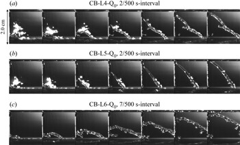
The image shown in figure 4 depicts the initial breakup process and rim surface instability. The breakup starts from the contact point between the left edge guide and roller, and propagates to the right through the edge guide and then the slit of the slot die. During the breakup, the rim acceleration is large because the rim mass is small, but as the rim grows, the acceleration decreases and it moves at an almost constant speed over time (see figure 3). Additionally, the dimensionless horizontal propagation speed of the rim calculated for CB- ${\rm L4}$,
 ${\rm L5}$, and
 ${\rm L6}$ from (3.21a,b) is 1.0, 0.96 and 0.78, respectively, which is consistent with the propagation speed of the rim presented in table 2. However, from figure 3, the liquid separates from the rim in the form of droplets as the rim propagates, and consequently, the rim radius remains constant on average.
Front image when the breakup occurs. Time lapse from the left to right, and the images in experiment CB- ${\rm L4}$,
 ${\rm L5}$ and
 ${\rm L6}$ are depicted at 2/500, 2/500 and 7/500-time intervals, respectively. The breakup occurs at the lower part of the leftmost edge guide.

2.3. Discussion on rim shape and stability
The rim shape and flow velocity inside the rim are discussed separately when the upper end of the rim is located on the edge guide and after it reaches the slot die. When the upper end of the rim is located on the edge guide, the radius of the rim increases as the rim propagates, and the liquid inside the rim moves vertically upward. In contrast, after the upper end of the rim reaches the slot die exit, the liquid flowing out of the slot die flows vertically downward along the rim due to the influence of gravity. Additionally, the rim shape is significantly affected by the thickness of the liquid curtain near the edge guide. Generally, the breakup speed near the edge guide is high (figure 4) because the liquid curtain is extremely thin near the edge guide, and the rim shape becomes linear as it propagates, as shown in figures 2 and 3. In experiment CB- ${\rm L6}$, ethanol was mixed in the working fluid, so it was considered that the edge guide had high wettability and hence the breakup from the edge guide was suppressed, and therefore the rim slope from the horizontal axis became small.
Regarding the stability of the rim, in experiment CA, no detachment of droplets from the rim was observed (figure 2), and in experiment CB, unevenness appeared on the rim surface and droplets separated from the rim (figure 2). If the occurrence of unevenness on the rim is due to Plateau–Rayleigh instability, the wavelength of the unevenness is approximately  $4.5 D$ for inviscid liquid (for e.g. Drazin & Reid Reference Drazin and Reid1982), where
 $D$ is the diameter of the rim. However, in the experiment, according to figure 4, the wavelength of the unevenness is approximately
 $1.5 D$ at the initial stage of rim generation, and after the rim reaches the slot die, the wavelength of the unevenness becomes longer and is approximately
 $4D$ according to figure 3.
Gravity also has the influence of reducing the horizontal propagation speed of the rim as the rim mass increases, causing the liquid in the rim to flow down. Additionally, the generation of the liquid lump on the rim in experiment CA and the detachment of the droplets from the rim in experiment CB, may have occurred from the influence of gravity, that is, Rayleigh–Taylor instability (for e.g. Drazin & Reid Reference Drazin and Reid1982). Because this instability causes the mass of the rim to reduce, it might be possible to evaluate the propagation speed of the rim from the force balance equation when the rim radius is constant and gravity is ignored.
3. Liquid-curtain rim shape
In this section, we analyse the governing equation of the rim of the liquid curtain based on the equation proposed by Entov & Yarin (Reference Entov and Yarin1984), but the shear force in the rim cross-section is ignored, as indicated by Roisman (Reference Roisman2010), and the gravitational force is included because gravity becomes dominant as the rim mass increases as it propagates. Here, we also assume that the cross-section of the rim is circular and its radius changes slowly spatially along the centreline of the rim.
This equation, however, is the equation with the Lagrangian variable as the independent one; hence, when analysing a flow with a fixed boundary, it is necessary to convert it to the Eulerian coordinate, and consequently, the equation becomes too complicated. Therefore, the objective of the analysis is selected step by step as follows:
(i) Find the rim shape, propagation speed and radius when a circular breakup occurs in the liquid curtain in the infinite region without gravity.
(ii) Find the rim shape, propagation speed and radius when a circular or elliptical breakup occurs in the liquid curtain in the infinite region with gravity.
(iii) Find the rim shape, propagation speed and radius of the liquid curtain in the strip-shaped region with fixed boundaries with gravity.
3.1. Governing equation for liquid-curtain rims
The basic equation in the present study was derived by Entov & Yarin (Reference Entov and Yarin1984) and Entov et al. (Reference Entov, Rozhkov, Feizkhanov and Yarin1986), and studied by Agbaglah et al. (Reference Agbaglah, Josserand and Zaleski2013) and Roisman (Reference Roisman2010), where the rim cross-section is circular and the flow within the rim cross-section is uniform. We consider only the rim associated with the breakup of the liquid curtain constrained in a vertical  $x$–
 $y$ plane, as shown in figure 5.


Let the position of the fluid particle in the centre of the rim take  $\boldsymbol {x} = \boldsymbol {X} \equiv (X (t, \zeta ), Y (t, \zeta ))$, where
 $t$ is time,
 $\zeta$ is a Lagrangian variable and
 $\boldsymbol {\tau }$ and
 $\boldsymbol {n}$ are the unit tangent and normal vectors, respectively, at the rim centreline in the following:
 \begin{equation} \boldsymbol{V}=\frac{\partial \boldsymbol{X}}{\partial t},\quad \boldsymbol{\tau}=\lambda^{{-}1}\frac{\partial \boldsymbol{X}}{\partial\zeta}, \quad \boldsymbol{n}=\lambda^{{-}1}\left(-\frac{\partial Y}{\partial\zeta},\frac{\partial X}{\partial\zeta}\right), \quad \lambda \equiv\left|\frac{\partial \boldsymbol{X}}{\partial\zeta}\right|, \end{equation}
where  $\boldsymbol {V}$ is the velocity of the fluid particle, and
 $\lambda$ is the scale factor of the transformation from the Lagrangian coordinate to the physical one. The connecting position between the rim and the curtain is
 $\boldsymbol {x}=\boldsymbol {X}_S=\boldsymbol {X}+R\,\boldsymbol {n}$, where
 $R$ is the radius of the rim. The continuity equation and Newton's second law with the fluid particle position as the unknown variable and the Lagrangian variable as the independent variable, are given by the following equations:
 \begin{gather} \frac{\partial\lambda A}{\partial t} +H_{S} \lambda_S(u_{Sn}-V_{Sn})=0,\end{gather}
 \begin{gather} \rho A\left\{\frac{\partial \boldsymbol{V}}{\partial t}+ \frac{\partial^{2} \boldsymbol{r}_G}{\partial t^{2}} -g (0,1) \right\}-\left( 2\sigma \boldsymbol{n}_S+h_{S}\boldsymbol{\varPi}_{S}\cdot\boldsymbol{n}_S \right) (1-\kappa R)\nonumber\\ +\,\rho h_{S}(u_{Sn}-V_{Sn})(\boldsymbol{u}_{S}-\boldsymbol{V}_S)(1-\kappa R)-\lambda^{{-}1} \frac{\partial \boldsymbol{F}}{\partial \zeta}=0, \end{gather}
where the gravitational force is included but the shear force in the rim cross-section is ignored, compared with the work of Roisman (Reference Roisman2010). Here,  $H$ and
 $\boldsymbol {u}$ are respectively the curtain thickness and velocity inside the curtain, the subscript ‘
 $S$’ denotes the value at the connecting position between the rim and the curtain,
 $\boldsymbol {V}_S=\partial \boldsymbol {X}_S/\partial t$,
 $V_{Sn}=\boldsymbol {V}_S\boldsymbol {\cdot } \boldsymbol {n}_S$,
 $u_{Sn}=\boldsymbol {u}_S\boldsymbol {\cdot } \boldsymbol {n}_S$,
 $A={\rm \pi} R^{2}$ and
 $\kappa$ is the curvature of the rim centreline given by
 \begin{equation} \kappa=\lambda^{{-}3}\left( \frac{\partial X}{\partial\zeta}\frac{\partial^{2} Y}{\partial\zeta^{2}} -\frac{\partial Y}{\partial\zeta}\frac{\partial^{2} X}{\partial\zeta^{2}} \right). \end{equation}
Here,  $\boldsymbol {r}_G$ denotes the position of the centre of gravity of the rim originating from the rim centre, given by
 \begin{equation} \boldsymbol{r}_G={-}\kappa \frac{I_b}{A}\boldsymbol{n},\quad I_b={\rm \pi}\frac{R^{4}}{4}, \end{equation}
where  $\boldsymbol {\varPi }$ denotes the internal stresses of the liquid curtain
 \begin{equation} \boldsymbol{\varPi}(x,y,t)=\left[\begin{array}{cc} \dfrac{\sigma}{2} \Delta H+2\mu \boldsymbol{\nabla}\boldsymbol{\cdot } \boldsymbol{u} + 2\mu \dfrac{\partial u_x}{\partial x} & \mu \left(\dfrac{\partial u_y}{\partial x}+ \dfrac{\partial u_x}{\partial y}\right) \\ \mu \left(\dfrac{\partial u_y}{\partial x}+ \dfrac{\partial u_x}{\partial y}\right) & \dfrac{\sigma}{2} \Delta H+2 \mu \boldsymbol{\nabla}\boldsymbol{\cdot } \boldsymbol{u} + 2\mu \dfrac{\partial u_y}{\partial y} \end{array}\right], \end{equation}
where  $\boldsymbol {u}=(u_x,u_y)$,
 $\varDelta$ and
 $\boldsymbol {\nabla }$ are respectively the two-dimensional Laplacian and nabla, and
 $\boldsymbol {\varPi }_S=\boldsymbol {\varPi }(X_S,Y_S,t)$. Finally,
 $\boldsymbol {F}$ is the tension force along the centreline of the rim which is given by
 \begin{equation} \boldsymbol{F}=P\boldsymbol{\tau}, \end{equation}
 \begin{align} P&=\sigma A \left[ R^{{-}1}\left\{1+\left(\frac{\partial R}{\lambda\partial\zeta}\right)^{2}\right\}^{{-}1/2}+\frac{\partial}{\lambda\partial\zeta}\left(\frac{\partial R}{\lambda\partial\zeta}\right) \left\{1+\left(\frac{\partial R}{\lambda\partial\zeta}\right)^{2}\right\}^{{-}3/2}\right]\nonumber\\ &\quad -6\mu A\delta -\mu W, \end{align}
 \begin{equation} \delta={-}\frac{1}{2}\left(\frac{\partial V_\tau}{\lambda\partial\zeta}-\kappa V_n\right), \quad W=h_S(V_{Sn} -u_{Sn})(1-\kappa R), \end{equation}
where  $V_\tau$ is the
 $\boldsymbol {\tau }$-component of
 $\boldsymbol {V}$, and
 $\mu \delta$ and
 $\mu W$ are respectively the viscous stresses due to the extension of the rim and expansion of the rim cross-section caused by the increase of the liquid volume supplied from the curtain.
To analyse the phenomena with fixed boundaries, the basic equations (3.2) and (3.3) with the Lagrangian variable  $\zeta$, need to be transformed to the equations with the Eulerian variable
 $x$. This variable transformation from
 $\zeta$ to
 $x$ is given by
 \begin{equation} x=X(t, \zeta(t, x)), \quad y=\eta(t,x)=Y(t, \zeta(t, x)), \end{equation}
where  $\zeta$ is the Lagrangian variable satisfying
 \begin{equation} \frac{\partial\zeta}{\partial t}+U(t,x)\frac{\partial\zeta}{\partial x}=0. \end{equation}
Differentiating the second expression in (3.10a,b) with respect to  $t$ and considering (3.11) leads to the kinematic boundary condition as follows:
 \begin{equation} \frac{\partial\eta}{\partial t}=V(t,x)-U(t,x)\frac{\partial\eta}{\partial x}, \end{equation}
where  $U=\partial X/\partial t$,
 $V=\partial Y/\partial t$.
The variable transformation of (3.2) and (3.3) from  $(t,\zeta )$ to
 $(t,x)$ can be achieved by the relations obtained from differentiating (3.10a,b) with respect to
 $t$ and
 $x$, where
 $(U,V, R,\eta )$ are the unknown functions. The equations after the change of variables, however, are complicated and it is difficult to find well-posed boundary conditions, because the basic equations include the second derivative of
 $t$ and the third derivative of
 $\zeta$. Therefore, in the next section, we first analyse the propagation of the rim of the liquid curtain with uniform flow in the infinite region. Next, in § 3.3, the equations with the Eulerian coordinate are approximated and the propagation of the rim is analysed for the flowing band-shaped liquid curtain.
In this paper, the length, velocity and time scales are non-dimensionalised by the curtain thickness  $H_0$, the flow velocity
 $u_0$ and
 $H_0/u_0$, respectively. Unless otherwise specified, physical quantities such as
 $t$,
 $x$,
 $X$,
 $Y$,
 $R$,
 $u_x$,
 $u_y$ and
 $\eta$ have been non-dimensionalised in the following sections.
3.2. The shape of the rim generated from the breakup of the liquid curtain in the infinite region
In this section, we analyse the rim propagation when the liquid curtain in the infinite region breaks without considering the existence of the edge guides, roller and slot die, but consider the region where the liquid curtain exists as shown in figure 5(b). First, a solution without gravity is obtained, then the line rim with gravity is discussed, and finally the rim propagation from the point source under gravity is numerically analysed.
3.2.1. Rim expanding from a point source without gravity
The solution of the circular rim without gravity is discussed in this section. This solution can be applied for the initial stage of the curtain breakup because the mass of the rim is small at the beginning of the breakup.
Let the axisymmetric solution of (3.2) and (3.3) be
 \begin{equation} X=h+X_0(t)-r(t)\cos\zeta_\theta,\quad Y=r(t)\sin\zeta_\theta,\quad R=R_0(t), \end{equation}
where  $\zeta _\theta$,
 $0\leqslant \zeta _\theta \leqslant 2{\rm \pi}$, is the Lagrangian variable,
 $h$ is the curtain height,
 $x=h+X_0(t)$ denotes the centre of the circular rim and
 ${\rm d}X_0/{\rm d}t=1$ for uniform flow. Here,
 $\zeta _\theta$ is positive in the clockwise direction. The elimination of
 $\zeta _\theta$ from (3.13a–c) leads to
 \begin{equation} y=\sqrt{r(t)^{2}-(x-h-X_0(t))^{2}}, \end{equation}
which describes a circle. The substitution of (3.13a–c) into (3.2) and (3.3) results in the equations for  $r(t)$ and
 $R_0(t)$. However, if the liquid curtain breaks from the point source and the rim becomes a torus, the relationship between
 $r(t)$ and
 $R_0(t)$ holds as follows:
 \begin{equation} {\rm \pi}\left\{R_0(t)+r(t)\right\}^{2} =2{\rm \pi}^{2} r(t) R_0(t)^{2}, \end{equation}
which is shown to satisfy the mass conservation law (3.2), and hence
 \begin{equation} R_0(t)=\frac{r(t)\left\{ 1+\sqrt{2{\rm \pi}\, r(t)} \right\}}{2{\rm \pi} r(t)-1}. \end{equation}
Equation (3.16) is applicable when  $r(t)>R_0(t)$, that is,
 $R_0(t)\geqslant 2/{\rm \pi}$ noting that the hole diameter of the cavity is zero when
 $R_0(t)={\rm \pi} /2$ and
 $r(t)={\rm \pi} /2$. Lastly, the dynamic equation (3.3) for the axisymmetric flow is
 \begin{align} & [ {\rm \pi}{R_0(t)}^{2}
r(t)\{4 r(t)^{2}- {R_0(t)}^{2}\}r''(t) +2{\rm \pi}
r(t)^{2} {R_0(t)}^{3} {R_0}''(t)\nonumber\\ &\quad
+\{ 4r(t)^{3} +4r(t)^{2} R_0(t) +2{\rm \pi} {R_0(t)}^{4}
\}{r'(t)}^{2} +2r(t)^{2}\{ 2r(t)+R_0(t)(2+{\rm \pi}
R_0(t))\}{{R_0}'(t)}^{2}\nonumber\\ &\quad
+4r(t)\{2r(t)^{2}+2 r(t) R_0(t)- {\rm \pi}
{R_0(t)}^{3}\}r'(t) {R_0}'(t)] \nonumber\\
&\quad -\frac{2\sqrt{2}Oh}{\sqrt{We}}r(t)
[\{r(t)+R_0(t)-3{\rm \pi} R_0(t)^{2}\}r'(t)
+\{r(t)+R_0(t)\}{R_0}'(t)]\nonumber\\ &\quad
-\frac{2}{We}r(t)^{2}[2r(t)-({\rm \pi}-2)R_0(t)]=0,
\end{align}
which shows the equilibrium condition of the inertial force, viscous force and surface tension.
To find an asymptotic solution after the breakup has progressed sufficiently, the substitution of (3.16) into (3.17), the variable transformation  $r'(t)=V_r(r(t))$ and the change of the variables from
 $(t, r(t))$ to
 $(r, V_r(r))$ lead to
 \begin{align} rV_r(r)\frac{{\rm d}V_r(r)}{{\rm d}t} +2V_r(r)^{2}-\frac{2}{We}=0,\quad V_r(r)=\sqrt{ \frac{1}{We} \left\{1-\left(\frac{r_I}{r}\right)^{4}\left(1-We\, {V_I}^{2}\right) \right\}}, \end{align}
which is satisfied for  $r\gg 1$, and the initial value is given as
 $V_r(r_I)=V_I$. Equation (3.18a,b) shows that
 $V_r(r)=1/\sqrt {We}$ and
 $r(t)=t/\sqrt {We}$ for
 $r\to \infty$, and hence, no viscous force influences the final propagation of the rim (see Savva & Bush Reference Savva and Bush2009)
3.2.2. Rim in rectangular region without gravity
For the solution of the rim obtained in the previous section, the value in the rectangular region  $0 \leqslant x \leqslant h$ is discussed in the following.
The approximation of (3.14) for  $X_0(t)\gg h$ and
 $r(t)\geqslant X_0(t)$ leads to
 \begin{equation} y=\sqrt{r(t)^{2}-X_0(t)^{2}} + \frac{X_0(t)}{\sqrt{r(t)^{2}-X_0(t)^{2}}}(x-h), \end{equation}
which means that the rim from the point source is linear in the rectangular region:  $0 \leqslant x \leqslant h$,
 $y \gg h$ and the horizontal propagation speed
 $c_H$ and angle
 $\psi$ between the line rim and
 $x$-axis are given as follows:
 \begin{equation} c_H=\frac{{\rm d}}{{\rm d}t}\sqrt{r(t)^{2}-X_0(t)^{2}},\quad \psi=\tan^{{-}1}\left(\frac{X_0(t)}{\sqrt{r(t)^{2}-X_0(t)^{2}}}\right). \end{equation}
Here, the limit  $t\to \infty$ leads to the following equations:
 \begin{equation} c_H=\sqrt{(1-We)/We}, \quad \psi=\tan^{{-}1}[\sqrt{We/(1-We)}]. \end{equation}
However, the propagation speed in the  $y$ direction at the initial stage of breakup, where the rim cannot be linearly approximated, is
 $\partial y/\partial t$, which can be obtained by differentiating (3.14) with respect to
 $t$. Additionally, the Lagrangian and Eulerian flow velocities in the rim are respectively given by
 \begin{gather} \frac{\partial X}{\partial t}=\frac{{\rm d}X_0(t)}{{\rm d}t}-\frac{{\rm d}r(t)}{{\rm d}t}\cos\zeta_\theta, \quad \frac{\partial Y}{\partial t}=\frac{{\rm d}r(t)}{{\rm d}t}\sin\zeta_\theta, \end{gather}
 \begin{gather} U=\frac{{\rm d}X_0(t)}{{\rm d}t}-\frac{{\rm d}r(t)}{{\rm d}t}\frac{x-h-X_0(t)}{-r(t)}, \quad V=\frac{{\rm d}r(t)}{{\rm d}t}\frac{y}{r(t)}. \end{gather}
Equation (3.23a,b) leads to  $U\to 0$ as
 $t\to \infty$ because
 $r(t)\to \infty$ in the region
 $0\leqslant x\leqslant h$.
Summing up the above results, the horizontal propagation speed of the rim is given by (3.21a,b) when gravity is ignored or the mass of the rim is small, even though the boundary conditions at the slot die, edge guides and rollers have been ignored in the present discussion.
3.2.3. Line rim solution with gravity
According to the experiment, the breakup that occurred from the contact point between the edge guide and roller propagates in the horizontal direction while maintaining an almost linear shape after reaching the slot die exit. Therefore, the solution of the rim with the following linear shape is given in the present section:
 \begin{equation} R=R_0(t), \quad X=\zeta_\ell +X_c(t), \quad Y=k X+Y_c(t), \end{equation}
where  $\zeta _\ell$,
 $-\infty <\zeta _\ell <\infty$ is the Lagrangian variable, and
 $k\equiv \tan \psi$ is a constant. Substituting (3.24a–c) into (3.2) and (3.3) and considering
 $S_0\gg 1$ for the developed rim, we obtain the approximated equations for the unknowns
 $R_0(t),\,X_c(t)$ and
 $Y_c(t)$ as follows:
 \begin{equation} \left.\begin{gathered} \frac{{\rm d}S_0(t)}{{\rm d}t}=\frac{k+{Y_c}'(t)}{\sqrt{1+k^{2}}},\\ \frac{{\rm d}{X_c}'(t)}{{\rm d}t}=\frac{Bo}{2 We}+\frac{-k+k We-k We {X_c}'(t)+We {Y_c}'(t)-We {X_c}'(t) {Y_c}'(t)}{We \sqrt{1+k^{2}}\, S_0(t)},\\ \frac{{\rm d}{Y_c}'(t)}{{\rm d}t}={-}\frac{Bo\, k}{2 We}+ \frac{1+k^{2}-k^{2} We-2k We {Y_c}'(t)-We {Y_c}'(t)^{2}}{We \sqrt{1+k^{2}}\, S_0(t)}, \end{gathered}\right\}\end{equation}
where  $S_0(t)$ is the area of the rim cross-section defined by
 $S_0(t)={\rm \pi} {R_0(t)}^{2}$ and ‘
 $'$’ denotes the time derivative. In the present section,
 $k$ is determined from the condition
 $U=\textrm {d}X_c/\textrm {d}t=0$ for
 $Bo=0$ as discussed in § 3.2.2, which leads to
 \begin{equation} k=\tan\psi=\sqrt{\frac{We}{1-We}}, \end{equation}
where  $\psi$ is the angle between the rim centreline and the
 $x$-axis. For instance, (3.26) leads to
 $\psi =29 ^{\circ }$ for
 $We=0.23$ in experiment CA-L1-
 $\textrm {Q}_{1}$, and
 $\psi =44 ^{\circ }$ for
 $We=0.49$ in experiment CB-L4-
 $\textrm {Q}_{0}$. In this case, the exact solution of (3.25) is given as follows:
 \begin{align} S_0(t)=\frac{t(12-Bo\, t)}{12 \sqrt{We}}, \quad {X_c}'(t)=\frac{Bo\, t\{6(3-We)-Bo\, t\}}{6We(12-Bo\, t)}, \quad {Y_c}'(t)=\frac{6(1-We)-Bo\, t}{6\sqrt{We(1-We)}}. \end{align}
It should be noted that (3.27a–c) is applicable for  $0 < t < 12/Bo$ because of
 $S_0(t) > 0$, and satisfies
 ${Y_c}' > 0$ for
 $t < t_{cr} \equiv 6(1-We)/Bo$. In this study, we consider the rim propagating to the positive
 $y$-direction, i.e.
 ${Y_c}' > 0$, then
 $t< t_{cr}$ and
 $R_0(t)< R_0(t_{cr})\equiv R_{cr}$. Here, we confirm that the exact solution (3.27a–c) of the approximate equation (3.25) takes a close enough value to the numerical solution of (3.16) and (3.17) when
 $t\gg 1$. Moreover, the effect of viscosity does not appear in the line rim because the governing equation of the line rim does not involve the Ohnesorge number.
3.2.4. Numerical solution of the rim generated from circular or elliptical breakup with gravity
The solution of the rim of the liquid curtain in the infinite region with gravity is numerically obtained in this section, and the propagation of the rim in the region of the curtain  $0 \leqslant x \leqslant h$ is discussed.
The derivatives with respect to  $\zeta _\theta$ in the governing equations (3.2) and (3.3) are discretised by a central finite difference scheme with quadratic accuracy, and the time-evolution equations for the unknown functions at the nodes are numerically solved. Here, the rim is spatially periodic in the circumferential direction, i.e.
 $0\leqslant \zeta _\theta \leqslant 2{\rm \pi}$. The initial value for the circular breakup is given by (3.13a–c), where
 $t$ is put to
 $t_I$ satisfying
 $R_0(t_I)=1$. For the elliptical breakup, the semi-major and semi-minor radii of the ellipse are set to the liquid-curtain height
 $h$ and
 $h/5$, respectively, and the initial radius of the rim is given by
 $R_0$ when the radius
 $r$ of the circular breakup becomes
 $h/5$.
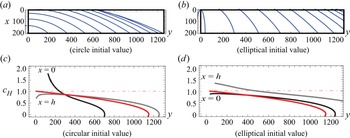
Figures 6(a) and 6(b) show the numerical results of the propagation of the circular and elliptical rims centred on  $x=h$ and
 $y=0$ in the rectangular region
 $0 \leqslant x \leqslant h, y \geqslant 0$ for the parameters in experiment CB-
 $\textrm {L}4$-
 $\textrm {Q}_{0}$. Compared with figure 4, the deceleration due to gravity of the rim is remarkable in this simulation, and the initial shape of the rim significantly affects the rim propagation. It should be noted that the calculation is performed for the liquid curtain in the infinite region, and the existence of the edge guide, slot die and roller have not been considered.
Rim shape and horizontal propagation speed ( $We=0.49, Oh=0.012,Bo=0.0013$). Panels (a,b) show the rim shape every 12/500 s. Panels (c,d) are the horizontal propagation velocities shown in (a,b), the black solid line:
 $c_H$ at the slot die exit (
 $x=0$), the grey solid line:
 $c_H$ at the roller surface (
 $x=h$), the red solid line:
 $c_H$ of (3.27a–c), the red dot-dashed line:
 $c_H$ of (3.21a,b).

Figures 6(c) and 6(d) show the horizontal velocities as a function of  $y$ at
 $x=0$ and
 $h$ depicted from figures 6(a) and 6(b). The red line in the figure is the analytical solution
 ${Y_c}'(t)$ of (3.27a–c), and the red chain line is the solution of (3.21a,b) where gravity is ignored. The rim propagation speed at the slot die exit (
 $x = 0$) is larger at the initial time because the rim touches the slot die exit. However, for the breakup starting from the elliptical shape, the propagation speed on the roller surface becomes larger.
From these results, the propagation speed of the rim is significantly affected by the initial shape of the rim, and the analytical solution of the approximate equation (3.27a–c) can roughly estimate the propagation speed of the rim in the presence of gravity. We also confirmed that the rim shape slightly changed even if the viscosity was varied from  $\mu = 0.01\ \textrm {cP}$ to
 $1\ \textrm {cP}$.
The same calculation is performed for the parameters in experiment CA- $\textrm {L1}$-
 $\textrm {Q}_{1}$, where the rim with the circular initial value moves vertically downward before reaching the slot die because the influence of gravity on the rim is more pronounced owing to the large liquid-curtain thickness.
As mentioned above, the long-term propagation of the rim in the present experiments cannot be explained from the rim in the liquid curtain in the infinite region. In the next section, we analyse the breakup of the liquid curtain in the band-shaped region  $0 \leqslant x \leqslant h$.
3.3. Shape of the rim due to the breakup of the liquid curtain in the band-shaped region
The problem with predicting the experimental results from the solution of the liquid curtain in the infinite region is that the infinite liquid curtain above the rim causes the mass of the rim to increase, and hence gravity slows down the propagation speed of the rim, which begins to fall vertically downward (see § 3.2.4). However, in the experiment, the volume flow rate flowing from the slot die to the rim is specified, hence the horizontal propagation speed is almost constant. Therefore, in this section, we perform an analysis in which the volume flow rate constraint is given as the boundary condition at the slot die exit.
To obtain conditions on fixed boundaries, it is necessary to convert the basic equations (3.2) and (3.3) to the Eulerian coordinate. As mentioned in § 3.1, the variable transformation makes the equation too long and complicated, and the method of obtaining the boundary conditions of the equation, including the third-order derivative for the spatial variable, is undecided. Therefore, in this section, assuming that the derivatives higher than the second order of the variables  $\psi (t,x)$, i.e.
 $\tan \psi =\partial \eta /\partial x$,
 $R(t,x)$,
 $U(t,x)$ and
 $V(t,x)$ with respect to
 $x$ are negligible, the following quasi-linear time evolution equations for
 $\psi$,
 $R$,
 $U$ and
 $V$, are used as the basic equations in this section:
 \begin{equation} \frac{\partial}{\partial t}\boldsymbol{X}+\boldsymbol{M}\frac{\partial}{\partial x}\boldsymbol{X}=\boldsymbol{f}, \quad \boldsymbol{X}={{}^{t}(\psi, R, U, V)}. \end{equation}
Here,  $\boldsymbol {M}$ is the coefficient matrix and f is the external force. Consequently,
 $\boldsymbol {M}$ and
 $\boldsymbol {f}$ become functions of
 $\psi$,
 $R$,
 $U$ and
 $V$ (see Appendix A). The first component in (3.28a,b) is the
 $x$-derivative of (3.12), and the other components are (3.2) and (3.3). Moreover, to avoid the complexity of the equation, the spatial differentiation of the flow velocity in the liquid curtain
 $\boldsymbol {u}$ is ignored, and the approximate expressions
 $\boldsymbol {u}_S\approx \boldsymbol {u}$ and
 $H_S\approx H\ \textrm {for}\ h\gg R$ are used; however, the dependence of the spatial variable
 $x$ on
 $\boldsymbol {u}$ and
 $H$ is retained. Although (3.28a,b) does not include
 $\eta (t,x)$ explicitly,
 $\eta (t,x)$ is determined from the kinematic condition equation (3.12) and
 $\partial \eta /\partial x = \tan \psi$ by
 \begin{equation} \eta(t,x)=\eta_{I0}+\int_0^{x} \tan\psi(t,x_I)\,{\rm d}\kern0.7pt x_I + \int_0^{t}(V(t_I,x)-U(t_I,x)\tan\psi(t_I,x)\,{\rm d}t_I, \end{equation}
where  $\eta _{I0}=\eta (0,0)$.
Next, the numerical calculations, along with the boundary and initial conditions, are discussed. After the upper end of the rim reaches the slot die exit, the flow in the rim is assumed to be determined from up- to downstream because  $U(t,0) >0$. The numerical method is to discretise the
 $x$-derivative of
 $\boldsymbol {X}$ in (3.28a,b) by the upwind finite difference scheme, and to solve the resultant ordinary differential equations numerically, where the value of
 $\boldsymbol {X}$ at each node is the unknown variable. The boundary condition at the upstream end is the volume flow rate of the liquid flowing into the rim from the slot die exit which is assumed to be proportional to the rim diameter, and is given as follows:
 \begin{equation} RU=\chi\frac{2}{\rm \pi} \quad {\rm or}\quad \frac{\partial}{\partial t}(RU)=0, \quad {\rm at}\ x=0 , \end{equation}
where  $\chi$ is a non-dimensional fitting parameter with order unity. The time evolution of
 $R$ at
 $x=0$ is determined by the second equation of (3.30), and that of
 $\psi$,
 $U$,
 $V$ at
 $x=0$ is given by (3.28a,b). Additionally, the values at the calculation points outside the boundary are extrapolated in this study.
The rim drawn in the bold yellow line in figures 2 and 3 is used as the initial rim for the present numerical simulation. Here,  $\psi =\psi _0+(\psi _h-\psi _0)x/h$,
 $R=R_M$,
 $\partial \eta /\partial t=\eta _{t0}$ and
 $U=2\chi /({\rm \pi} R_M)$, where
 $\psi _0$,
 $\psi _h$,
 $R_M$ and
 $\eta _{t0}$ are estimated from the high-speed camera images, and
 $V$ is determined to satisfy (3.12).
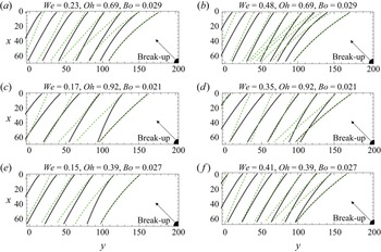
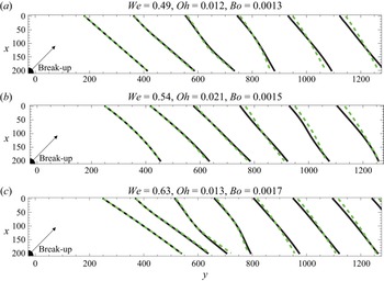
Figures 7 and 8 show the simulation results for the experiments by Coater A and Coater B by setting  $\chi = 2$. In these figures, the solid black and green dotted line show the cases for free fall:
 $u_x = \sqrt {1 + Bo \, x/We}, u_y = 0$ and uniform flow:
 $u_x = 1, u_y = 0$, respectively. The average propagation speed explains the experimental results, the rim radius does not increase monotonically with propagation (see figure 9), and the rim propagates until the liquid curtain disappears from the region sandwiched by the edge guides. Additionally, the propagation speed of the rim is not constant, for example, it accelerates after decelerating (for instance, Oron et al. (Reference Oron, Davis and Bankoff1997) and Balestra et al. (Reference Balestra, Brun and Gallaire2016)). This is because the Rayleigh–Taylor instability causes a large mass to flow vertically downward (see figure 9). This Rayleigh–Taylor instability is observed in CA-
 $\textrm {L1}$-
 $\textrm {Q}_{2}$, CA-
 $\textrm {L2}$-
 $\textrm {Q}_{2}$, and CA-
 $\textrm {L3}$-
 $\textrm {Q}_{2}$ in figure 2.
Time evolution of rim shape (calculation results for experiment CA). Equation (3.28a,b) was solved under the boundary condition (3.30) and the rim shape was plotted every 12/500 s. The initial value of the rim shape is given by the yellow thick line of figure 2. In the figure, the black line shows the value when the liquid curtain accelerates due to gravity and the curtain becomes thinner in the fall direction. The green dotted line shows the value when the curtain does not accelerate and the thickness is constant.

Time evolution of the rim shape (calculation results for experiment CB). Equation (3.28a,b) was solved under the boundary condition (3.30) and the rim shape was plotted every 12/500 s. The initial value of the rim shape is given by the thick yellow line of figure 3. In the figure, the black line shows the value when the liquid curtain accelerates because of gravity and the curtain becomes thinner in the fall direction. The green dotted line shows the value when the curtain does not accelerate and the thickness is constant.

Time evolution of the rim radius shown in figures 7 and 8. From the left, the results of the numerical simulation for CA- $\textrm {L1}$-
 $\textrm {Q}_1$, CA-
 $\textrm {L1}$-
 $\textrm {Q}_2$ and CB-
 $\textrm {L4}$-
 $\textrm {Q}_{0}$ are shown, respectively. The initial condition was
 $R = \textrm {const.}$, and the rim shape is plotted every 12/500 s. In the figure, time elapses in the order of black, blue, red, orange, green and purple solid lines.

In the experiment, the rim slope increases as the rim propagates; in other words, the horizontal propagation speed on the roller surface is greater than that on the slot die exit. Conversely, it decreases in the present simulations. However, for the rim of the liquid curtain in the infinite region, the slope increases as the rim propagates, exhibiting the same tendency as in the experiment (see figure 6).
Comparing the initial rim shape in the uniform flow and the free fall, the slope from the vertical line in the uniform flow becomes larger than that in the free fall, as shown in figure 7; hence, the value in the uniform flow approaches the experimental one at the initial time. Although the slope of the rim in the uniform flow decreases at the later time, this means that the initial condition is influential in the rim propagation. In experiment CB,  $Fr$ is large, the influence of the gravitational acceleration of the liquid curtain is small and there is no big difference in the rim shape between the black solid line and the green dotted line in figure 8. However, the rim in the experiment is considered to accelerate faster than the results of this simulation because the liquid is separated from the rim as droplets.
Next, the undecided parameter  $\chi$ included in the boundary condition of (3.30) is explained. In this simulation,
 $\chi$ has been set to 2, but in case of
 $\chi \lessapprox 2$, the upwind difference scheme becomes unstable and the solution cannot be found. In case of
 $\chi \gtrapprox 2$, the propagation speed of the rim becomes smaller and the average propagation speed deviates from the experimental value. As described above, there are unclear points in the initial and boundary conditions, and future studies are required.
Figure 9 shows the time evolution of the rim radius in the simulation of CA- $\textrm {L1}$-
 $\textrm {Q}_1$, CA-
 $\textrm {L1}$-
 $\textrm {Q}_2$ and CB-
 $\textrm {L4}$-
 $\textrm {Q}_0$. If the initial value of the rim radius is given uniformly in space, then it changes rapidly. In this simulation, the initial value of the calculation is obtained from the experimental value of the rim in the propagated state. Hence, the initial value should be determined so that the time change rate of the rim radius at the initial stage becomes small. However, it was difficult to improve the accuracy of the initial value because it was estimated from the image.
Finally, the instability of Plateau–Rayleigh observed in the experiment (figure 3) is not expressed by (3.28a,b) because the basic equation (3.28a,b) involves only the first-order derivative with respect to  $x$. The formation of droplets from the rim is discussed in the next section.
4. Stability of the circular and line rims
Figures 3 and 4 show that the rim surface becomes uneven after the breakup and the droplets separate from the rim. The wavelength of this unevenness is approximately the rim diameter at the beginning of the breakup, and becomes several times the rim diameter as the rim propagates. Conversely, in experiment CA, as shown in figure 2, the rim is smooth and no unevenness is observed. In this section, we explain the occurrence of unevenness on the rim surface by analysing the stability of the rim of the liquid curtain in the infinite region.
The target range of flow in the stability analysis is shown in figure 10(a), which is divided into two parts, i.e. the initial and developed stages. The former and latter main streams are respectively given by the solutions of the rim developed from the circular breakup (§ 3.2.4) and the line rim (§ 3.2.3). In this section, we discuss the stability for the flow with the values of  $We$,
 $Oh$ and
 $Bo$ shown in figure 10, and explain the physical phenomena observed in experiments CA-
 $\textrm {L1}$-
 $\textrm {Q}_1$ and CB-
 $\textrm {L4}$-
 $\textrm {Q}_0$.
Time evolution of the shape and radius of the rim. (a) Schematic diagram of a circular rim in the initial stage and a line rim in the developed stage. (b) Time evolution of the rim radius in the initial stage of a uniform liquid curtain in the infinite region. Each curve corresponds to the rim shape shown in (a). Here,  $\zeta _\theta =0$ and
 ${\rm \pi}$ are respectively the upper and lower ends of the rim.

Figure 10(b) shows the radius  $R$ of the rim at the initial stage of the breakup discussed in § 3.2. The minimum value of the rim radius is
 $R_0(t)={\rm \pi} /2$, the radius of the rim centreline is
 $r_0(t)={\rm \pi} /2$ and the hole diameter of the breakup is zero at this time. Subsequently, when the rim radius is, for example,
 $R = 2$, the curvature of the rim centreline becomes
 $1/r\approx 1/20$ according to (3.16), which can be ignored compared with the curvature of the rim cross-section. From the above discussions, the stability analysis is divided into the following three steps:
(i) Linear stability analysis of a circular rim at the time of the breakup of a liquid curtain in the infinite region without gravity (
 $R \geqslant {\rm \pi}/2$).
(ii) Numerical analysis of the disturbance on the circular rim when a circular breakup occurs in the liquid curtain in the infinite region with gravity.
(iii) Numerical analysis of the disturbance on the line rim when a straight breakup occurs in a liquid curtain in an infinite region with gravity.

4.1. Disturbance in the Lagrangian coordinate
In the linear stability analysis, the perturbation equation is derived from the basic equation and is analysed to obtain the time evolution of the disturbance. Here, the present basic equations (3.2) and (3.3) are described by the Lagrangian variable as an independent variable; therefore, we discuss the relationship between the stability analysis of the equations in the Eulerian and Lagrangian notations. Setting the flow velocity in the Eulerian fixed coordinate as  $U(t,x)$, the Euler–Lagrange relation and solution including the disturbance are respectively expressed as
 \begin{equation} \frac{\partial X}{\partial t}=U(t,X), \quad X=X_0(t,\zeta_\ell)+\epsilon X_f(t,\,\zeta_\ell), \quad U=U_0(t,x)+\epsilon U_f(t,x). \end{equation}
The first-order equation of  $\epsilon$ in the Euler–Lagrange relation leads to the following relation between
 $U_f(t,X_0)$ and
 $X_f(t, \zeta _\ell )$:
 \begin{equation} \frac{\partial X_f}{\partial t}=\frac{\partial U_0}{\partial x}(t,X_0)X_f + U_f(t,X_0). \end{equation}
Substitution of the line rim solution  $X_0=\zeta _\ell +X_c(t)$ into the zeroth order the Euler–Lagrange relation leads to
 $U_0(t,x)={X_c}'(t)$, and putting the solution in Lagrangian coordinate by
 $X_f=\textrm {Re}[A_X(t)\exp ({\textrm {i}\alpha _\ell \zeta _\ell })]$, then (4.2) leads to the solution of the disturbance equation in the Eulerian coordinate as follows:
 \begin{equation} U_f(t,x)={\rm Re}\left[{A_X}'(t)\exp({{\rm i}\alpha_\ell(x-X_c(t))})\right], \end{equation}
where  $\alpha _\ell$ is the wavenumber in the rim length direction and we use the relation
 $x=\zeta _\ell +X_c(t)$. Equation (4.3) shows that the instability of the Lagrangian mainflow leads to that of the Eulerian one for the line rim noting that
 $X_c(t)$ is a real function. This argument holds true for the circular rim with a uniform rim radius. However, in the case that the main stream
 $U_0$ depends on
 $x$, these instabilities do not match.
4.2. Linear stability of the rim generated by the breakup of a point source
In this section, we discuss the stability of the rim generated from the breakup of a point source in the uniform liquid curtain in the infinite region. Here, for the sake of simplicity, the initial disturbance is given only to the rim radius  $R$, not to the rim centreline
 $(X,Y)$.
4.2.1. Linear stability of the circular rim without gravity
The linear stability of the circular rim without gravity is considered, and the change in instability with the increase of the rim radius as a function of time, is discussed. When gravity is ignored, the main stream is given by (3.16) and (3.17), and the solutions, including the disturbance, are set to the following equations:
 \begin{equation} \left.\begin{gathered} R=R_0(t)+ \epsilon R_f(t, \zeta_\theta),\\ X=h+X_0(t)- r(t) \cos\zeta_\theta + \epsilon X_f(t, \zeta_\theta), \quad Y= r(t) \sin\zeta_\theta + \epsilon Y_f(t, \zeta_\theta). \end{gathered}\right\} \end{equation}
Substituting the above equations into the governing equations (3.2) and (3.3) and taking the first-order term of  $\epsilon$, the linear disturbance equations are obtained and its solutions are given as follows:
 \begin{equation} \left.\begin{gathered} R_f=A_R(t)\cos(\alpha_\theta\zeta_\theta),\\ X_f=A_n(t)\cos((\alpha_\theta-1)\zeta_\theta)+A_p(t)\cos((\alpha_\theta+1)\zeta_\theta),\\ Y_f=A_n(t)\sin((\alpha_\theta-1)\zeta_\theta)-A_p(t)\sin((\alpha_\theta+1)\zeta_\theta), \end{gathered}\right\} \end{equation}
where  $\alpha _\theta$ is the circumferential wavenumber of the circular rim and a symmetrical disturbance with respect to the
 $x$-axis is considered. The reason why
 $X_f$ and
 $Y_f$ are given by the linear sum of the wavenumber components
 $\alpha _\theta -1$ and
 $\alpha _\theta +1$ in the above equations is that the disturbances in the
 $x$ and
 $y$-directions are respectively given by
 $X_f\propto r_f \cos \zeta _\theta$ and
 $Y_f\propto r_f \sin \zeta _\theta$, according to the coordinate transformation, where the radial disturbance of the rim centreline
 $r_f$ is proportional to
 $\cos (\alpha _\theta \zeta _\theta )$.
The initial value of the main stream is the value at the moment when the breakup occurs:  $R_0(0)=2/{\rm \pi}$,
 ${R_0}'(0)=0$, and the initial conditions of the linear disturbance equations are given by
 $A_R(0)=1$,
 $A_n(0)=A_p(0)=0$ and
 ${A_n}'(0)={A_p}'(0)=0$.
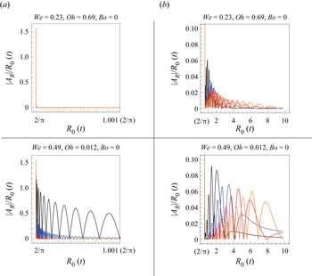
Figure 11(a,b) shows the solution of the linear disturbance equation for a given circumferential wavenumber  $\alpha _\theta$. Here, the horizontal axis is the rim radius
 $R_0(t)$ instead of the time
 $t$, and the vertical axis is
 $|A_R|/R_0(t)$, i.e. the absolute value of the disturbance amplitude normalised by the rim radius. Figure 11(a) depicts an enlarged waveform of the spike around
 $R(0)=2/{\rm \pi}$ in figure 11(b).
Time evolution of the disturbance on the circular rim without gravity. The amplitude of the disturbance with wavenumber  $\alpha _\theta$ is shown as a function of
 $R_0(t)$. The upper and lower panels show the results respectively for
 $We=0.23$ and
 $Oh=0.69$, in experiment LA-
 $\textrm {L1}$-
 $\textrm {Q}_{1}$ and
 $We=0.49$ and
 $Oh=0.012$ in experiment LB-
 $\textrm {L4}$-
 $\textrm {Q}_0$. Here, the vertical axis is the disturbance amplitude normalised by the rim radius
 $R_0 (t)$, the horizontal axis is the rim radius
 $R_0(t)$ and disturbances of
 $\alpha _\theta =10$, 20, 30 and
 $40$ are respectively indicated by black, blue, red and orange lines. (a) Rapid attenuation from the initial value. (b) Amplification of each wavenumber component.

The upper and lower panels of figure 11 describe the amplitude of the disturbance in  $We=0.23,\,Oh=0.69$ and
 $Bo=0$ for experiment LA-
 $\textrm {L1}$-
 $\textrm {Q}_1$ and in
 $We=0.49$,
 $Oh=0.012$ and
 $Bo=0$ for experiment LB-
 $\textrm {L4}$-
 $\textrm {Q}_0$. For the top panels, the disturbance is rapidly attenuated at the moment of breaking and then amplified, but it decays again after passing
 $R_0(t)\approx 2$. However, for the bottom panels, the high-frequency vibration appears at the moment of breaking and it is rapidly attenuated and then amplified. The value of
 $R_0 (t)$, giving the maximum amplitude of the disturbance, increases with
 $\alpha _\theta$; these values are given by
 $(\alpha _\theta,R_0(t))=(10, 1.5),(20, 3.5),(30, 4.5)$ and
 $(40, 6.0)$, which lead to the wavelength of the most unstable mode of
 $0.6, 2.1,2.5$ and
 $3.1\, \textrm {mm}$, respectively, and which is calculated from
 $\alpha _\ell =\alpha _\theta /r(t)$ and (3.16). This low wavenumber shift accompanying the propagation of the rim qualitatively explains the rim unevenness shown in figure 4. Because
 $Bo=0$ in this section, the disturbance amplification that appears here is due to the Plateau–Rayleigh instability (Rayleigh Reference Rayleigh1882).
Summing up the above results, the disturbance is attenuated while vibrating at a high frequency at the initial stage of the occurrence of the breakup, and then amplified and attenuated again as the rim radius increases. Additionally, the rim diameter at which the maximum disturbance occurs differs depending on the wavenumber in the circumferential direction.
4.2.2. Frozen flow stability analysis without gravity for $R\geqslant {\rm \pi}/2$

To observe the behaviour of the small disturbance near  $R_0(t)=2/{\rm \pi}$ and the amplification of the wavenumber mode in
 $1\leqslant R(t) \leqslant 10$, we assume the exponential solution,
 $\exp (st)$, for the solution of the linear disturbance equation discussed in § 4.2.1, by considering the coefficient of the unknown functions in this equation to be a constant (frozen flow stability analysis). Consequently, the eigenvalue
 $s$ becomes a solution of a fifth-order algebraic equation, and it depends parametrically on
 $t$ and
 $\alpha _\theta$. Here, we discuss the case where
 $We=0.49$,
 $Oh=0.012$ and
 $Bo=0$. Solving this algebraic equation numerically yields one real eigenvalue (
 $s \geqslant 0$) and two sets of complex conjugate eigenvalues. One conjugate eigenvalue whose real part is negative (see figure 12a) explains the numerical results in figure 11(a), where high-frequency vibration occurs at the initial time and decays rapidly. The real part of the other conjugate eigenvalue, which is designated by
 $s_r$, is positive and depends parametrically on
 $\alpha _\theta$ and
 $t$. Hence, the disturbance amplitude is evaluated by the following Wentzel–Kramers–Brillouin (WKB) approximation:
 \begin{equation} A_R(t)\propto\exp\left[\int_{t_I}^{t} s_r(\alpha_\theta, {t_I})\,{\rm d}t_I\right]\equiv A_{WKB}(t). \end{equation}
Figure 12(b) shows the normalised amplitude  $A_{W\!K\!B}(t)/R_0(t)$ for
 $\alpha _\theta =10$, 20, 30 and
 $40$ as a function of
 $R_0(t)$ in the case of
 $We=0.49$,
 $Oh=0.012$ and
 $Bo=0$. The amplitudes of the modes with
 $\alpha _\theta = 20$ and
 $30$ attain the maximum at
 $R_0(t)\simeq 6$ and
 $9$, respectively. Comparing these rim radii with the numerical results shown in figure 11(b), they have similar tendencies, although the values here are greater.
Eigenvalue  $s$ calculated from the frozen stability analysis of the circular rim for
 $We=0.19$,
 $Oh=0.013$ and
 $Bo=0$. The solution of the eigenvalue equation leads to one real and two sets of complex conjugate eigenvalues. (a) The real and imaginary parts of the eigenvalue where the real part is negative at
 $t = 0$, as a function of the circumferential wavenumber
 $\alpha _\theta$. (b) Amplitude calculated by substituting the eigenvalues whose real part is positive into (4.6).

4.2.3. Numerical calculation of the disturbance propagation on the circular rim with gravity
In the absence of gravity, the disturbance on the rim oscillates over time, the rim remains circular and expands in the radial direction, where eventually, the disturbance disappears as the rim radius increases. In this section, when gravity is considered, the propagation of the disturbance on the rim is evaluated by numerical calculation, where the rim radius increases non-uniformly along the circumferential direction.
We give the initial values of the rim centreline, radius and velocities by the following equations using the rim solution from (3.13a–c):
 \begin{equation} \left.\begin{gathered} X|_{t=0}=h-r_I(R_I)\cos\zeta_\theta,\quad Y|_{t=0}=r_I(R_I)\sin\zeta_\theta,\quad R=R_I\left(1+\eta(\zeta_\theta)\right),\\ \left.\frac{{\rm d}X}{{\rm d}t}\right|_{t=0}=1-\frac{1}{\sqrt{We}}\cos\zeta_\theta,\quad \left.\frac{{\rm d}Y}{{\rm d}t}\right|_{t=0}=\frac{1}{\sqrt{We}}\sin\zeta_\theta, \end{gathered}\right\} \end{equation}
where  $R_I$ and
 $r_I$ are the initial values of
 $R$ and
 $r$, respectively, and
 $\eta (\zeta _\theta )$ is the disturbance of the rim radius. The radial velocity of the breakup is given by the asymptotic solution of (3.18a,b), and the rim radius
 $r_I$ is determined from the conservation of mass equation (3.16) given by
 \begin{equation} r_I(R_I)={-}R_I+{\rm \pi} {R_I}^{2}+R_I\sqrt{{\rm \pi} R_I({\rm \pi} R_I-2)}. \end{equation}
The initial value of the disturbance amplitude of the rim radius is given by a small quantity as follows:
 \begin{equation} \eta(\zeta_\theta)=0.0001\cos\zeta_\theta, \end{equation}
and the numerical calculation is performed for  $\zeta _\theta =10$, 20,
 $30$ and
 $40$.
Figure 13 shows the absolute value of the disturbance amplitude for each wavenumber component as a function of the rim mean radius  $\bar {R}(t)$ defined by
 $(R_{max}(t)+R_{min}(t))/2$. The basic equation in this section is nonlinear, but it is confirmed that the disturbance amplitude is extremely small and the given disturbance wavenumber is predominant. The calculation result shows the amplification in the linear stage. At the initial time, the disturbance oscillates with high frequency and attenuates for all wavenumbers. Subsequently, low-frequency oscillations appear, and the disturbance amplitude increases monotonically. However, the disturbance amplitude for
 $We=0.23$,
 $Oh=0.69$ and
 $Bo=0.029$ is approximately 0.2 times that of
 $We=0.49$,
 $Oh=0.012$ and
 $Bo=0.013$, but the process of the initial attenuation, amplification and monotonic increase of the disturbance is similar. The former oscillations and the latter monotonic increase of the disturbance amplitude in figure 13 are respectively caused by the breakup of the circular rim and the Rayleigh–Taylor instabilities. This is because these oscillations do not appear for the instability of the line rim, as indicated later in figure 15(a), and comparison between figures 11(b) and 13 shows that the latter monotonic increase of the disturbance amplitude is from the effect of gravity, which is the Rayleigh–Taylor instability.
Time evolution of disturbances on the rim generated by the breakup of a point source with gravity for various initial wavenumbers  $\alpha _\theta$. The left and right-hand figures show the results for
 $We=0.23$,
 $Oh=0.69$ and
 $Bo=0.029$ and
 $We=0.49$,
 $Oh=0.012$ and
 $Bo=0.013$, respectively. The vertical axis shows
 $|A_R|/\bar {R}(t)$, and the horizontal axis shows the rim mean radius
 $\bar {R}(t)$.

As the breakup radius increases, the rim length direction wavenumber of the initial given circumferential wavenumber decreases in inverse proportion to the breakup radius, the method of decomposing the disturbance into the circumferential wavenumber component and obtaining the time evolution of the amplitude has a limit in its application when the breakup radius becomes large. However, as the breakup radius increases, the instability depending on the curvature of the rim centreline decreases, so the instability of the rim after the breakup progresses and is discussed by considering if the rim as a local straight line is possible.
4.3. Stability of the line rim
We evaluate the stability of the line rim introduced in § 3.2.3. The main stream of this solution is put to  $(R_0(t),X_0(t,\zeta _\ell ),Y_0(t,\zeta _\ell ))$ and the solution with the disturbance is given as follows:
 \begin{equation} \left.\begin{gathered} R=R_0(t)+\epsilon A_R(t) \exp({{\rm i}\alpha_\ell\zeta_\ell}),\\ X=X_0(t,\zeta_\ell)+\epsilon A_X(t) \exp({{\rm i}\alpha_\ell\zeta_\ell}), \quad Y=Y_0(t,\zeta_\ell)+\epsilon A_Y(t) \exp({{\rm i}\alpha_\ell\zeta_\ell}). \end{gathered}\right\} \end{equation}
Substituting the above equations into (3.2) and (3.3), and taking the first-order terms of  $\epsilon$, we obtain the linear disturbance equations. In this section, we first analyse the stability of the rim for a small disturbance with the frozen stability analysis, and then find the numerical solution of the linear disturbance equations with variable coefficients. Finally, the direct numerical calculation of (3.2) and (3.3) is performed for the line rim with initial disturbances.
The variable  $\zeta _\ell$ is briefly explained in the following. Considering two fluid particles denoted by
 $\zeta _\ell$ and
 $\zeta _\ell +\textrm {d}\zeta _\ell$ in the Lagrangian coordinate, then the distance between these two fluid particles in the Eulerian coordinate is calculated from (3.24a–c) and is given by
 $\textrm {d}\zeta _\ell \sqrt {1+k^{2}}$. Therefore, the wavelength in the Eulerian coordinate is equal to
 $\sqrt {1+k^{2}}$
 $\times$ (the wavelength in the Lagrangian coordinate).
4.3.1. Frozen flow stability analysis
Substituting (4.10) into the rim governing equations (3.2) and (3.3), and taking the first-order term for  $\epsilon$, the linear disturbance equations are obtained. Because the linear disturbance equations are ordinary differential equations with variable coefficients for
 $t$, it is difficult to solve them analytically. Therefore, we assume the exponential solution
 $\exp (st)$ and discuss the stability by determining the eigenvalue
 $s$ as in § 4.2. The eigenvalue equation is a fifth-order algebraic equation of
 $s$, and the eigenvalue with the maximum amplification exponent among the five eigenvalues is put to
 $s_M$. Here,
 $s_M$ depends parametrically on
 $t$, but, as in the previous section, we will discuss the stability by considering
 $s_M$ to be a function of
 $R_0(t)$ instead of
 $t$. For spatially periodic disturbances, the wavenumber and amplification exponent giving the maximum amplification of the disturbance for real
 $\alpha _\ell$ and
 $R_0(t)$ are obtained and the linear stability is discussed. However, in the amplification of the localised disturbance, the wavenumber and rim radius are analytically connected to the complex region, and the value at the saddle point of
 $s_M$ in the complex plane
 $(\alpha _\ell, R_0(t))$, determines the absolute instability (for e.g. Chomaz Reference Chomaz2005).
Figure 14 shows the most unstable wavenumber, amplification exponent and wave celerity for fixed values of  $R_0(t)$ and
 $Bo=0.0013$,
 $We=0.49$ and
 $Oh=0.012$. The black dots in the figure denote the real value
 $\alpha _\ell$ that maximises
 $s_{M\,r} = Re [s_M]$ and the corresponding value of
 $s_{M\,r}$ at that time
 $t$, i.e.
 $R=R_0(t)$. The open circles in the figure show the real part of
 $\alpha _\ell$, which satisfies
 $\partial s_M/\partial \alpha _\ell =0$, to decide the absolute or convective instability and the corresponding value of
 $s_{M\,r}$. Figure 14(b) shows that disturbances on the line rim are absolutely unstable in the Lagrangian coordinate because
 $s_{M\,r}> 0$ for
 $R_0(t)\geqslant 5$ at the saddle point on the complex plane. In the same analysis, the saddle point satisfying
 $\partial s_M/\partial \alpha _\ell =\partial s_M/\partial R_0=0$ is obtained as
 $R_0(t)=R_{ab}=9.4+0.64\,\textrm {i}$,
 $\alpha _\ell =\alpha _{ab}=0.071-0.013\,\textrm {i}$,
 $s_M=s_{ab}=0.0042-0.0017\,\textrm {i}$. Here, the subscript ‘
 $ab$’ represents the absolute instability. As described above, according to the linear global stability analysis, the instability is excited at
 $R_0\approx 8.9$, and the wavenumber and angular frequency at which the growth rate is the maximum, are
 $\alpha _\ell \approx 0.071$ and
 $s_{M\,i}=\textrm {Im}[s_M]\approx -0.017$.
Eigenvalue of the most unstable mode calculated from the frozen stability analysis of the line rim for  $We=0.49$,
 $Oh=0.012$,
 $Bo=0.0013$ and
 $R_{cr}=27.7$. (a) Wavenumber, (b) amplification exponent and (c) celerity. The black dots are values when
 $\alpha _\ell$ is real, whereas the open circles are the real part of the absolutely unstable wavenumber, the amplification factor
 $s_ {M \, r}$ and wave celerity
 $c_M$ evaluated by
 $\alpha _{\ell \,r}$ and
 $s_{M\,i}$.

4.3.2. Numerical solution of the linear disturbance equation
The asymptotic analysis in § 4.3.1 can be applied under the condition where the variable coefficient of the linear disturbance equation changes slower than the time change of the solution. To verify the validity of this condition and to evaluate the physical factors of the rim instability, we solve the linear disturbance equation numerically for  $\alpha _\ell =0.02$, 0.04, 0.06,
 $0.08$ and
 $0.10$ referring to figure 14(a). Here, the initial value of the numerical solution is given by
 $A_R(0)=1,A_X(0)=A_Y(0)=0$ and
 ${A_X}'(0)={A_Y}'(0)=0$.
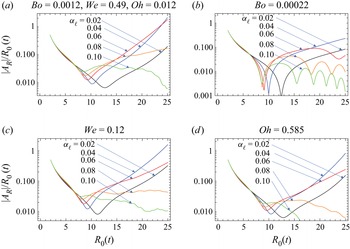
Figure 15(a) shows the absolute value of the normalised disturbance amplitude  $|A_R|/R_0(t)$ as a function of
 $R_0(t)$ for
 $Bo=0.0013$,
 $We=0.49$ and
 $Oh=0.012$, and for
 $\alpha _\ell = 0.02 \sim 0.10$. Figure 15(b–d) shows the results of the sensitivity analysis by changing one of the parameters in (a) to
 $Bo \to Bo/6$ (
 $g \to g/6$) in (b),
 $We \to We/2$ (
 $Q_0 \to Q_0/2$) in (c) and
 $Oh \to 50 Oh$ (
 $\mu \to 50 \mu$) in (d). From these figures, the disturbance amplitude is clearly smaller in figure 15(b), and therefore the instabilities shown in figures 14 and 15 are considered to be due to the Rayleigh–Taylor instability. Additionally, the effects of viscosity and surface tension are prominent on the high wavenumber side, i.e. for
 $\alpha _\ell \gtrapprox 0.06$.
Numerical solutions of the linear disturbance equation for the line rim. The perturbation equation based on (4.10) is solved numerically. (a) The absolute value of the normalised disturbance amplitude  $|A_R|/R_0(t)$ as a function of
 $R_0(t)$ for
 $Bo=0.0013$,
 $We=0.49$ and
 $Oh=0.012$; (b–d)
 $R_0(t)$ vs
 $|A_R|/R_0(t)$. Sensitivity analysis by changing one of the parameters in (a), i.e. (b)
 $Bo \to Bo/6$, (c)
 $We \to We/2$, (d)
 $Oh \to 50 Oh$.

Next, we compare the results of figures 14 and 15(a). Figure 15(a) shows that the disturbance amplitude changes from a decrease to an increase at  $R_0(t)\approx 10$, and the wavenumber at which the amplification exponent, i.e. the slope of the curve, takes the maximum near
 $R_0(t)=10$ at
 $\alpha _\ell =0.04\sim 0.06$, and near
 $R_0(t)\sim 25$ at
 $\alpha _\ell =0.04$. Figure 14 shows that the disturbance decays for
 $R_0(t)<5$, the absolute instability occurs at
 $R_0(t)=9.4$, the corresponding wavenumber is given by
 $\alpha _\ell \sim 0.07$ and the maximum amplification at
 $R_0(t)\sim 25$ occurs at
 $\alpha _\ell =0.4$. From the above, the results from the frozen stability analysis are consistent with the numerical solution.
The actual wavelength is estimated from the wavenumber  $\alpha _\ell =0.04$, which gives the maximum amplification exponent as equal to
 $2{\rm \pi} /(0.04\sqrt {1-We})\times H_0 \approx 2.2\ \textrm {cm}$. This prediction is valid because approximately two lumps have been observed on one rim in figure 3.
4.3.3. Numerical calculation of the disturbance propagation on the line rim
In the linear stability analysis, the interaction between wavenumbers does not occur, and even if the rim radius  $R$ changes, the wavenumber of disturbance
 $\alpha _\ell$ does not change. However, the wavenumber that maximises the linear amplification factor depends on the rim radius, and it is considered that the interaction among wavenumbers affects the development of the disturbance during the propagation process. Therefore, we perform numerical calculations of the nonlinear basic equations (3.2) and (3.3) to evaluate the time evolution of disturbances consisting of a large number of wavenumber modes at the initial time. The initial value of the numerical calculation is given by adding the disturbance to the solution of the line rim equations (3.24a–c) and (3.27a–c) as follows:
 \begin{align} \left.\begin{gathered} R|_{t=0}=R_0(t_I) + R_f(\zeta_\ell), \quad X|_{t=0}=\zeta_\ell+X_c(t_I),\quad Y|_{t=0}=k\left(\zeta_\ell+X_c(t_I)\right) +Y_c(t_I),\\ X'|_{t=0}={X_c}'(t_I), \quad Y'|_{t=0}=k{X_c}'(t_I) +{Y_c}'(t_I). \end{gathered}\right\} \end{align}
The disturbance  $R_f(\zeta _\ell )$ is given by the following equation so as to include many wavenumber components:
 \begin{equation} \frac{R_f(\zeta_\ell)}{R_I}=\frac{\epsilon_R }{n_L}\sum_{m=1}^{n_L}\cos\left(\frac{m\alpha_{\ell I}}{n_L}\zeta_\ell+\phi_m\right). \end{equation}
Here,  $\epsilon _R$ and
 $n_L$ denote the amplitude and the number of spatial modes of the disturbance, respectively, and the parameter
 $t_I$ included in the initial condition (4.11) is given so that
 $R_0(t_I) = R_I$ is satisfied, where
 $R_I$ is the rim radius at
 $t = 0$, and
 $\alpha _{\ell I}$ is given to include the most unstable wavenumber. Additionally, the calculation area is
 $0 \leqslant \zeta _\ell < L$,
 $L$ is
 $n_L$ times the disturbance wavelength
 $2{\rm \pi} /\alpha _{\ell I}$ (
 $0\leqslant \zeta _\ell \leqslant L$). The phase
 $\phi _m\in [0, 2{\rm \pi} )$ is a random variable that follows a Gaussian distribution. The reason why
 $\epsilon _R$ is divided by the number of modes
 $n_L$ in (4.12) is to avoid an increase in the amplitude of
 $R_f(\zeta _\ell )/R_I$ when the stochastically generated phases are close to each other.
Figure 16 shows the time evolution of the wavenumber spectrum for  $n_L=20$,
 $\epsilon _R=0.01$. From (4.12), the minimum and maximum values of the wavenumber included at
 $t=0$ are
 $\alpha _{\ell I}/n_L$ and
 $\alpha _{\ell I}$, respectively. Hence, the waveform with the maximum wavenumber was divided into 32 in this numerical calculation. The panels (a) and (b) of figure 16 are the solutions for
 $We=0.23$,
 $Oh=0.69$,
 $Bo=0.029$,
 $\alpha _I=0.2$ and
 $R_I=2$ and
 $We=0.49$,
 $Oh=0.012$,
 $Bo=0.0013$,
 $\alpha _I=0.1$ and
 $R_I=5$, respectively. The value of
 $\epsilon _R$ is the same in both cases, and the initial spectrum shown by the black line is flat regardless of the wavenumber.
Time evolution of the wavenumber spectrum of the disturbance on the line rim. In the figure, black, blue, red, orange, green and purple lines are the values at  $t=0$,
 $0.2 t_f$,
 $0.4 t_f$,
 $0.6 t_f$,
 $0.8 t_f$ and
 $t_f$, respectively. The left and right figures show the spectrum for
 $We=0.23$,
 $Oh=0.69$,
 $Bo=0.029$ and
 $R_0(0)=2$ and
 $R_0(t_f)=7$ and
 $We=0.49$,
 $Oh=0.012$,
 $Bo=0.0013$,
 $R_0(0)=5$ and
 $R_0(t_f)=25$, respectively, where
 $t_f$ is the time when
 $R_0(t_f)=7$ or
 $R_0(t_f)=25$ is satisfied.

The wavenumber  $\alpha _{\ell M}$ that gives the maximum amplitude decreases as the rim radius
 $R_0(t)$ increases, and
 $\alpha _{\ell M}=0.12$ for
 $We=0.23$,
 $Oh=0.69$ and
 $Bo=0.029$, whereas
 $\alpha _{\ell M}=0.05$ for
 $We=0.49$,
 $Oh=0.012$ and
 $Bo=0.0013$ at
 $R_0(t) \approx R_{cr}$. Hence, the actual wavelength that gives the maximum growth rate is evaluated from
 $2{\rm \pi} /(\alpha _\ell \sqrt {1-We})\times H_0$ by approximately
 $1.8\ \textrm {cm}$ for both experiments CA-
 $\textrm {L1}$-
 $\textrm {Q}_{1}$ and CB-
 $\textrm {L4}$-
 $\textrm {Q}_{0}$.
Comparing the maximum amplitude of the spectrum, the amplification rate in the parameters of experiment CA- $\textrm {L1}$-
 $\textrm {Q}_{1}$ is smaller than that of experiment CB-
 $\textrm {L4}$-
 $\textrm {Q}_{0}$, and the former value remains small even if the rim radius reaches the critical value
 $R_{cr}$, whereas in the latter case, the nonlinearity appears and the slope of the rim surface also increases.
5. Discussion and conclusions
We conducted experiments and theoretical analysis in curtain coating with regard to the propagation of the rim which was generated by the breakup of the liquid curtain occurring at the contact between the edge guide and roller, and discussed the shape, propagation speed and stability of the rim in the low-Weber-number range. The governing equation in the present study is based on Entov's equation (Entov & Yarin Reference Entov and Yarin1984), and ignores the shear force in the rim cross-section, but considers the gravitational force.
First, we solved the governing equation in the infinite region, and predicted the shape and propagation speed of the rim observed in this experiment. Consequently, it was found that the rim did not propagate horizontally when gravity was considered, and the experimental results could not be predicted from the rim of the liquid curtain in the infinite region (see figure 6). Therefore, by converting the governing equation in the Lagrangian coordinate to that in the Eulerian one, deriving a quasi-linear differential equation involving only the first-order derivatives from the converted equation and finding a solution that satisfies the volume flow rate boundary condition at the slot die exit, the propagation speed of the rim could be roughly explained (see figures 7, 8).
For the stability of the rim, the experiments were performed when the Ohnesorge number was much smaller than 1 and of the order of unity. When the Ohnesorge number was much smaller than 1, unevenness appeared on the rim surface and the droplets separated from the rim (see figure 3), whereas when it was of the order of unity the centreline of the rim became convex downward vertically and the liquid lump flowed down through the rim although it did not generate droplets (see figure 2).
To explain the experimental results, the stability of the circular and line rims was examined by the numerical solution of the linear disturbance equation and eigenvalues based on the frozen stability analysis. From the stability analysis of the circular rim without gravity, the unevenness on the rim that appears in the initial stage of the breakup in experiment CB- $\textrm {L4}$-
 $\textrm {Q}_{0}$ is due to the Plateau–Rayleigh instability, whereas the amplification factor of the disturbance on the rim decreases sharply as the rim radius increases for the dimensionless parameters in experiment CA-
 $\textrm {L1}$-
 $\textrm {Q}_{1}$, where the clear unevenness was not observed (see figure 11).
Additionally, in the presence of gravity, the Rayleigh–Taylor instability appears after the Plateau–Rayleigh instability appears on the circular rim at the initial stage of the breakup, and the disturbance amplitude increases monotonically without oscillations (see figures 13 and 15). Moreover, from the stability analysis of the line rim with gravity, the wavenumber of the most unstable mode decreased as the rim radius increased, and the wavelength of this wavenumber was approximately  $1.8\ \textrm {cm}$ both for the rim with a radius of
 $2.1\, \textrm {mm}$ in experiment CA-
 $\textrm {L1}$-
 $\textrm {Q}_{1}$ and
 $2.5 \ \textrm {mm}$ in experiment CB-
 $\textrm {L4}$-
 $\textrm {Q}_{0}$.
At the developed stage of the curtain breakup, when  $Oh$ is much smaller than 1, the droplets separate from the rim and the propagation speed of the rim is almost constant, whereas when the order of
 $Oh$ is 1, the liquid lump flows down on the rim and the propagation speed of the rim decreases. Frozen stability analyses is useful to predict the wavelength of the most unstable mode and to verify the validity of numerical analysis, but cannot distinguish between the Plateau–Rayleigh and Rayleigh–Taylor instabilities.
Supplementary movies
Supplementary movies are available at https://doi.org/10.1017/jfm.2022.547.
Acknowledgements
The first author would like to thank Professor T. Tsuda and Dr K. Nakano for their informative discussions on curtain coating techniques.
Funding
This work was supported in part by a Grant-in-Aid for Scientific Research (A)22248025 from JSPS (Principal Investigator; Professor Y. Adachi).
Declaration of interests
The authors report no conflict of interest.
Author contributions
H.K. derived the theory and G.S. and M.R. performed the experiment.
Appendix A. Approximation to the quasi-linear equation
The basic equations (3.2) and (3.3) are time-evolution equations for the rim radius and the velocity of the fluid particle in the Lagrangian coordinate system. The variable transformation (3.10a,b) gives the equations for the dependent variables  $(\psi, R, U, V)$ in the Eulerian coordinate system
 $(t, x)$, which have high-order nonlinearity and contain high-order derivatives with respect to
 $t$ and
 $x$. According to the present experimental results, after the upper end of the rim reaches the slot die exit, the rim propagates while maintaining an almost linear shape (see figures 2 and 3), and hence we assume that differentiations of
 $(\psi, R, U, V)$ with respect to
 $x$ are small, i.e.
 $O(\partial ^{n}/\partial x^{n})= \epsilon ^{n}$, where
 $n$ is an integer and
 $\epsilon$ indicates the size of the value, and derive the approximate equations where only the zeroth and first derivatives of these dependent variables with respect to
 $t$ and
 $x$ are considered.
In this appendix, in order to express the formula concisely, the derivative is expressed by the subscripts as follows:  $\partial f/\partial x=f_{,x}$,
 $\partial f/\partial t=f_{,t}$,
 $\partial ^{2} f/\partial t\partial x=f_{,tx}$,
 $\partial ^{2} f/\partial t^{2}=f_{,tt}, \ldots$, etc. Moreover, we assume that the curtain stream velocity
 $u_x$ and thickness
 $H$ are weakly dependent on
 $x$ so that their
 $x$ derivatives are ignored, and, to avoid confusion, the value for the liquid curtain is written by
 $u_x \equiv \hat {u}$ and
 $H \equiv \hat {H}$. Furthermore, to make the physical meaning clear, the following dimensionless density, surface tension coefficient, viscosity coefficient and gravitational acceleration are respectively introduced in the present manipulations by
 \begin{equation} \tilde{\rho}=1, \quad \tilde{\sigma}=\frac{Oh}{2 We}, \quad \tilde{\mu}=\sqrt{ \frac{Oh We}{2} }, \quad \tilde{g}=\frac{Bo Oh}{2 We}. \end{equation}
First, we derive the quasi-linear equations for  $\psi$ and
 $R$ respectively from the kinematic condition (3.12) and the law of conservation of mass (3.2), and secondly, use these results to obtain the quasi-linear equations for
 $U$ and
 $V$ from the equations of motion (3.3).
First, differentiating (3.12) with respect to  $x$ and considering
 $\partial \eta /\partial x \equiv \tan \psi$, then the time-evolution equation of
 $\psi$ is given as follows:
 \begin{equation} \psi_{,t}+U \psi_{,x}+ U_{,x} \cos\psi \sin\psi- V_{,x}\cos^{2}\psi =0. \end{equation}
The above equation yields  $O(\psi _{,t})= \epsilon$ because
 $\psi _{,t}$ is represented by the linear superposition of the
 $x$-derivative of the dependent variables. Next, the variable transformation of (3.10a,b) on the continuity equation (3.2) leads to
 \begin{align} & 4\{\hat{H}-R(2{\rm \pi}+\hat{H} \psi_{,x}\cos\psi)\}R_{,t}\cos\psi-4{\rm \pi} R^{2}\psi_{,t} \sin\psi\nonumber\\ &\quad -4R [{\rm \pi} R U\sin\psi +\hat{H}\{(\hat{u}-U)\sin\psi +V\cos\psi\} \cos^{2}\psi]\psi_{,x}\nonumber\\ &\quad -4{\rm \pi} R^{2}\,U_{,x}\cos\psi + 4\hat{H}\{ (\hat{u}-U)\sin\psi +V\cos\psi\} \cos\psi + O(\epsilon^{2})=0,\end{align}
where  $O(R_{,t})=1$ has been considered. Similarly, the equations of motion (3.3) in the Eulerian coordinate system are respectively given for the
 $x$ and
 $y$-directions in the following. Approximate equation of motion for the
 $x$-direction is
 \begin{align} & \tilde{\rho}\left[ \vphantom{\frac{{\rm \pi} R^{2}}{4}}{\rm \pi}R^{2} (U_{,t} + U U_{,x}- \tilde{g} ) + \hat{H}({-}1+2R_{,x} \sin \psi )U^{2} \sin \psi\right. \nonumber\\&\quad-\hat{H} \{ \hat{u} \sin \psi + V\cos\psi+(\hat{u} \cos^{2} \psi -V \cos\psi \sin\psi)R_{,x} + R_{,t} \}(\hat{u}+ R_{,t} \sin \psi)\nonumber\\ &\quad+\frac{\hat{H} U}{2}\left\{4\hat{u}\sin\psi +\hat{u}({-}1+3\cos 2\psi)R_{,x} +2V(1-2R_{,x} \sin\psi)\cos\psi\right. \nonumber\\ &\quad\left. +\,(3-\cos 2\psi)(1-R_{,x}\sin\psi)R_{,t} \right\}+\hat{H}R \left\{ (\hat{u}-U)\sin\psi +V\cos\psi + R_{,t}
\right\} \nonumber\\ &\quad \left.\times \left\{ -\psi_{,t}+ (\hat{u}-2U +R_{,t}\sin\psi )\psi_{,x} \right\}\cos\psi + \frac{{\rm \pi} R^{2}}{4} (R R_{,tt} +{R_{,t}}^{2})\psi_{,x}\sin2\psi \right] \nonumber\\ &\quad + \tilde{\sigma} \left[ 2\sin\psi +({\rm \pi}-2)({-}R_{,x}\cos\psi +R\psi_{,x}\sin\psi)\cos\psi \right]+\tilde{\mu} \hat{H}\left[ \left\{ (\hat{u}-U)\cos 2\psi\right.\right.\nonumber\\ &\quad\left.\left. +\,U-V \sin 2\psi-R_{,t}\sin\psi \right\}\psi_{,x} + \psi_{,t} + R_{,tx}\cos\psi \right]\cos\psi + O(\epsilon^{2})=0,\end{align}
and that for the  $y$-direction is
 \begin{align} & \tilde{\rho} \left[ {\rm \pi}
R^{2} V_{,t} -\frac{\hat{H}}{4}\{ U({-}5\cos\psi+\cos
3\psi)R_{,x} +2U(\sin 2\psi +2R \psi_{,x}\sin^{3}\psi)\right. \nonumber\\
&\quad-4\hat{u} R_{,x}\cos^{3}\psi-2\hat{u}\sin 2\psi(1-R
\psi_{,x}\cos\psi) +2V R_{,x}\cos\psi \sin 2\psi\nonumber\\
&\quad -2V(3+\cos 2\psi)(1-R\psi_{,x}\cos\psi)\} R_{,t}
+\hat{H}(1-R\psi_{,x}\cos\psi) {R_{,t}}^{2} \cos\psi
\nonumber\\ &\quad +R\{ {\rm \pi}RU\sec^{2}\psi
-\hat{H}(\hat{u}-U)\sin^{2}\psi -\hat{H}V\sin\psi \cos\psi\}\psi_{,t} -\hat{H}RR_{,t}\psi_{,t}\sin\psi
\nonumber\\ &\quad +\hat{H}V^{2}
(1-R_{,x}\sin\psi-R\psi_{,x}\cos\psi)\cos\psi +\hat{H}
V\{ \hat{u} R_{,x}\cos^{2}\psi-U(\sin\psi-R_{,x})\nonumber\\
&\quad +\hat{u}(1-R
\psi_{,x}\cos\psi)\sin\psi \} +{\rm \pi} R^{2}
U(U_{,x}\tan\psi +U \psi_{,x}\sec^{2}\psi) \nonumber\\
&\quad + \hat{H}U(\hat{u}-U)R_{,x}\cos\psi \sin\psi
+\hat{H}RU(U-\hat{u}) \psi_{,x}\sin^{2}\psi \nonumber\\
&\quad \left.-\, \frac{{\rm \pi} R^{2}}{2 } (R R_{,tt}
+{R_{,t}}^{2})\psi_{,x}\cos^{2}\psi
\vphantom{\frac{\hat{H}}{4}}\right]-\tilde{\sigma}[
2\cos\psi+({\rm \pi}-2)R_{,x}\sin\psi\cos\psi\nonumber\\
&\quad +({\rm \pi}-2)R \psi_{,x}\cos^{2}\psi]
+\tilde{\mu} \left[ \frac{\hat{H}}{2} \{
2R_{,t}\cos^{2}\psi +2\hat{u}\cos\psi \sin 2\psi+2V\cos\psi
\cos 2\psi\right. \nonumber\\ &\quad
\left.+\,U(\sin\psi -\sin 3\psi)
\}\vphantom{\frac{\hat{H}}{2}}+\hat{H}(\psi_{,t}+R_{,tx}\cos\psi)\sin\psi
\vphantom{2R_{,t}\cos^{2}\psi +2\hat{u}\cos\psi
\sin 2\psi+2V\cos\psi \cos 2\psi}\right] + O(\epsilon^{2})=0,
\end{align}
where  $O(U_{,t})=1$ and
 $O(V_{,t})=1$ have been considered, noting that
 $O(R_{,t})=1$,
 $O(U_{,t})=1$ and
 $O(V_{,t})=1$ are consistent with the basic equations (3.2) and (3.3). Because (A2)–(A5) are not linear for variables
 $(\psi _{,t},R_{,t},U_{,t},V_{,t})$ and
 $(\psi _{,x},R_{,x},U_{,x},V_{,x})$, further approximations to obtain the time-evolution form are performed in the next step.
In order to obtain the quasi-linear equations for the dependent variables  $(\psi, R, U, V)$ from (A2)–(A5), their time-evolution form is expressed as
 \begin{align} \psi_{,t} = F_{\psi 0}+ F_{\psi 1}, \quad R_{,t}= F_{R0}+ F_{R1}, \quad U_{,t}= F_{U0}+ F_{U1}, \quad V_{,t}= F_{V0}+ F_{V1}, \end{align}
where  $(F_{\psi 0},F_{R0}, F_{U0},F_{V0})$ is the
 $O(1)$-function of the variables
 $\psi$,
 $R$,
 $U$ and
 $V$ only, and
 $(F_{\psi 1},F_{R1}, F_{U1},F_{V1})$ is a linear function of the variables
 $\psi _{,x}$,
 $R_{,x}$,
 $U_{,x}$ and
 $V_{,x}$, which has the order of
 $\epsilon$. Approximation (A6a–d) is possible because the basic equations (3.2) and (3.3) are a time-evolution equation of
 $(R(t,\zeta ), X(t,\zeta ), Y(t,\zeta ))$ and we consider the terms up to the first-order derivative with respect to
 $x$ in the present calculations. In order to obtain
 $(F_{\psi 0},F_{R0},F_{U0},F_{V0})$ explicitly, all the
 $x$-derivatives in (A2)–(A5) are put to 0, i.e. taking
 $O(1)$ terms only, and the resulting linear algebraic equations for unknowns
 $(F_{\psi 0},F_{R0},F_{U0},F_{V0})$ are solved as follows:
 \begin{equation} F_{\psi 0}=0, \end{equation}
 \begin{equation} F_{R0}=\frac{\hat{H}(-\hat{u}+U)\sin\psi -\hat{H}V \cos\psi}{\hat{H}-2 {\rm \pi}R},\\ \end{equation}
 \begin{align} F_{U0}&=\frac{1}{{\rm \pi}
\tilde{\rho} R^{2}(\hat{H}-2{\rm \pi} R)^{2}}\left[
\vphantom{+\frac{{\rm \pi}\hat{H}R}{2}}{\rm \pi}
\tilde{\rho}\tilde{g}R^{2}(\hat{H}- 2{\rm \pi} R)^{2}
-{\rm \pi}\tilde{\rho}\hat{H} R V(\hat{H}-4{\rm \pi}
R)(\hat{u}-U)\cos\psi\right.\nonumber\\ &\quad
+{\rm \pi}\tilde{\rho}\hat{H}^{2} R V (-\hat{u}-U)\cos 3\psi
-\frac{\rm \pi}{2}\tilde{\rho} \hat{H}^{2} R
\{(\hat{u}-U)^{2} -V^{2} \}\sin 3\psi\nonumber\\
&\quad -2\tilde{\sigma} \hat{H}^{2} \sin\psi + 4{\rm \pi}^{2}
R^{2} \{{-}2 \tilde{\sigma} +\tilde{\rho}\hat{H}\hat{u}^{2}
+\tilde{\rho}\hat{H}U(U-2\hat{u}) \} \sin\psi
\nonumber\\ &\quad \left. +\,\frac{{\rm \pi}\hat{H}R}{2} \{
16\tilde{\sigma} -\tilde{\rho}\hat{H}\hat{u}^{2}
+\tilde{\rho}\hat{H}(2\hat{u}U-U^{2}
+V^{2})\}\sin\psi \right],
\end{align}
 \begin{align} F_{V0}&=\frac{1}{{\rm \pi}
\tilde{\rho} R^{2}(\hat{H}-2{\rm \pi} R)^{2}}[{-}2{\rm \pi}
\tilde{\rho}\hat{H} R V(\hat{H}\cos 2\psi +2{\rm \pi}
R)(\hat{u}-U)\sin\psi\nonumber\\ &\quad + {\rm \pi}
\hat{H} R\{{-}8\tilde{\sigma} -\tilde{\rho}
\hat{H}\hat{u}^{2}(1-\cos 2\psi)-2\tilde{\rho}\hat{H}
U(U-2\hat{u})\sin^{2}\psi\} \cos\psi\nonumber\\
&\quad +2\tilde{\sigma} (\hat{H}^{2} + 4{\rm \pi}^{2}
R^{2})\cos\psi +{\rm \pi}\tilde{\rho}\hat{H}R V^{2}({-}4{\rm \pi}
R\cos\psi +\hat{H} \sin\psi \sin 2\psi)].
\end{align}
Furthermore, solving (A2) and (A3) for unknowns  $\psi _{,t}$ and
 $R_{,t}$ algebraically, the
 $O(\epsilon )$-terms of these solution lead to
 $(F_{\psi \, 1}$,
 $F_{R\, 1})$ as follows:
 \begin{equation} F_{\psi\, 1}={-}U\psi_{,x} -U_{,x} \cos\psi \sin\psi + V_{,x} \cos^{2} \psi, \end{equation}
 \begin{align} F_{R\, 1}&={-}\frac{2 {\rm \pi}\hat{H} R^{2}\left\{(\hat{u}-U)\sin\psi +V \cos\psi \right\}\cos\psi}{(\hat{H}-2{\rm \pi} R)^{2}}\,\psi_{,x}\nonumber\\ &\quad - \frac{ \hat{H}\hat{u} \cos^{2} \psi - 2{\rm \pi} RU +\hat{H}(U\sin\psi -V\cos\psi) \sin\psi}{\hat{H}-2{\rm \pi} R} R_{,x}\nonumber\\ &\quad +\frac{{\rm \pi} R^{2}\cos^{2} \psi}{\hat{H}-2{\rm \pi} R}\, U_{,x} + \frac{{\rm \pi} R^{2} \sin 2\psi}{2(\hat{H}-2{\rm \pi} R)}\, V_{,x}. \end{align}
Next, we will explain how to find  $(F_{U \, 1}, F_{V \, 1} )$. Noting that the time derivative terms contained in (A4) and (A5) are
 $U_{,t}$,
 $V_{,t}$,
 $\psi _{,t}$,
 $R_{,t}$,
 $R_{,tx}$ and
 $R_{,tt}$, the second-order derivative terms
 $R_{,tx}$ and
 $R_{,tt}$ must be represented by only the first-order derivative terms, that is achieved by differentiating
 $R_{,t}= F_{R0}+ F_{R1}$ respectively with respect to
 $x$ and
 $t$ as follows:
 \begin{equation} R_{,tx}= \frac{\partial F_{R0}}{\partial\psi}\psi_{,x} +\frac{\partial F_{R0}}{\partial R}R_{,x} +\frac{\partial F_{R0}}{\partial U}U_{,x} +\frac{\partial F_{R0}}{\partial V}V_{,x}+O(\epsilon^{2}), \end{equation}
 \begin{align} R_{,tt}&= \frac{\partial F_{R0}}{\partial\psi}\psi_{,t} +\frac{\partial F_{R0}}{\partial R}R_{,t} +\frac{\partial F_{R0}}{\partial U}U_{,t} +\frac{\partial F_{R0}}{\partial V}V_{,t}\nonumber\\ &\quad + \frac{\partial F_{R1}}{\partial\psi_{,x}}\psi_{,xt} +\frac{\partial F_{R1}}{\partial R_{,x}}R_{,xt} +\frac{\partial F_{R1}}{\partial U_{,x}}U_{,xt} +\frac{\partial F_{R1}}{\partial V_{,x}}V_{,xt}+O(\epsilon^{2})\nonumber\\ &=\frac{\partial F_{R0}}{\partial\psi}F_{\psi 1} +\frac{\partial F_{R0}}{\partial R}(F_{R0}+ F_{R1}) +\frac{\partial F_{R0}}{\partial U}(F_{U0}+ F_{U1}) +\frac{\partial F_{R0}}{\partial V}(F_{V0}+ F_{V1})\nonumber\\ &\quad + \frac{\partial F_{R1}}{\partial R_{,x}} \left( \frac{\partial F_{R0}}{\partial\psi}\psi_{,x} +\frac{\partial F_{R0}}{\partial R}R_{,x} +\frac{\partial F_{R0}}{\partial U}U_{,x} +\frac{\partial F_{R0}}{\partial V}V_{,x} \right)\nonumber\\ &\quad +\frac{\partial F_{R1}}{\partial U_{,x}} \left( \frac{\partial F_{U0}}{\partial\psi}\psi_{,x} +\frac{\partial F_{U0}}{\partial R}R_{,x} +\frac{\partial F_{U0}}{\partial U}U_{,x} +\frac{\partial F_{U0}}{\partial V}V_{,x} \right)\nonumber\\ &\quad +\frac{\partial F_{R1}}{\partial V_{,x}}\left( \frac{\partial F_{V0}}{\partial\psi}\psi_{,x} +\frac{\partial F_{V0}}{\partial R}R_{,x} +\frac{\partial F_{V0}}{\partial U}U_{,x} +\frac{\partial F_{V0}}{\partial V}V_{,x} \right)+O(\epsilon^{2}), \end{align}
where  $O(\psi _{,xt})=\epsilon ^{2}$ has been applied. By substituting (A13) and (A14) into (A4) and (A5), and taking
 $O(\epsilon )$ terms from these equations, the resulting linear algebraic equations for
 $(F_{U1},\,F_{V1})$ are solved analytically and their solution is given as follows:
 \begin{align}
F_{U1}&={-}\frac{1}{{\rm \pi}\hat{\rho}R^{2}}
\left[\vphantom{\left({F_{R0}}^{2}+R F_{R0} \frac{\partial
F_{R0}}{\partial R} +R F_{U0} \frac{\partial
F_{R0}}{\partial U} +R F_{V0} \frac{\partial
F_{R0}}{\partial V} \right)} {\rm \pi}\hat{\rho} R U U_{,x} +2
\hat{\rho} \tilde{H} R_{,x} U^{2} \sin^{2}\psi \right.\nonumber\\
&\quad \left. -\,({\rm \pi}-2)\hat{\sigma}(R_{,x}\cos\psi -R \psi_{,x}
\sin\psi)\cos\psi\right.\nonumber\\
&\quad +\hat{\mu}\tilde{H} \left\{ F_{\psi 1} +U\psi_{,x} +
\frac{\partial F_{R0}}{\partial R} R_{,x}\cos\psi +
\frac{\partial F_{R0}}{\partial
U}U_{,x}\cos\psi\right.\nonumber\\
&\quad + \frac{\partial F_{R0}}{\partial V} V_{,x}\cos\psi + \frac{\partial
F_{R0}}{\partial \psi}\psi_{,x} \cos\psi +(\tilde{u}-U)
\psi_{,x}\cos 2\psi\nonumber\\
&\quad \left. -\,(F_{R0}+2V\cos\psi)\psi_{,x} \sin\psi \vphantom{\frac{\partial F_{R0}}{\partial
R}}\right\}\cos\psi
+\hat{\rho}\tilde{H}
R\left\{F_{R0}+V\cos\psi+(\tilde{u}-U)\sin\psi\right\}\nonumber\\
&\quad \times \left\{{-}F_{\psi
1}+(\tilde{u}-2U+F_{R0}\sin\psi)\psi_{,x}\right\}\cos\psi
-\frac{\hat{\rho}\tilde{H}}{2} U \left\{ F_{R1}(\cos
2\psi-3)+\tilde{u} R_{,x}\right.\nonumber\\ &\quad \left.
+\,(3 F_{R0}+4V\cos\psi)R_{,x}\sin\psi
-(3\tilde{u}+F_{R0}\sin\psi-F_{R1})R_{,x} \cos
2\psi\right\}\nonumber\\ &\quad -\hat{\rho}
\tilde{H}\{F_{R1}(F_{R0}+V\cos\psi
+\tilde{u}\sin\psi)\sin\psi + (\tilde{u}+
F_{R0}\sin\psi)\nonumber\\ &\quad \times(F_{R1}+ \tilde{u} R_{,x} \cos^{2}\psi -V
R_{,x}\sin\psi \cos\psi)\}\nonumber\\ &\quad \left. +\,
\frac{{\rm \pi}\hat{\rho}}{4} R^{2} \left({F_{R0}}^{2}+R F_{R0}
\frac{\partial F_{R0}}{\partial R} +R F_{U0} \frac{\partial
F_{R0}}{\partial U} +R F_{V0} \frac{\partial
F_{R0}}{\partial V} \right) \psi_{,x} \sin 2\psi \right],
\end{align}
 \begin{align} F_{V1}&={-}\frac{1}{2{\rm \pi}
\hat{\rho}R^{2}}\left[ \vphantom{\left( {F_{R0}}^{2} +R
F_{R0}\frac{\partial F_{R0}}{\partial R} +R
F_{U0}\frac{\partial F_{R0}}{\partial U} +R
F_{V0}\frac{\partial F_{R0}}{\partial V}
\right)}2{\rm \pi}\hat{\rho} R^{2} U U_{,x}\tan\psi + \hat{\rho}
\tilde{H} F_{R1}V(3+\cos 2\psi) +2\hat{\rho}\tilde{H}UV
R_{,x}\right.\nonumber\\ &\quad +2{\rm \pi}\hat{\rho} R^{2}
U(F_{\psi 1}+U\psi_{,x})\sec^{2}\psi -2({\rm \pi}-2)\hat{\sigma}
(R\psi_{,x}\cos\psi +R_{,x}\sin\psi)\cos\psi\nonumber\\
&\quad +2\hat{\mu}\tilde{H}\left\{ (F_{\psi 1}-U\psi_{,x}
\cos 2\psi)\sin\psi +(F_{R0}+2
\tilde{u}\sin\psi)\psi_{,x}\cos^{2}\psi\right.\nonumber\\
&\quad +V\psi_{,x}\cos 2\psi \cos\psi+\frac{\partial
F_{R0}}{\partial\psi} \psi_{,x}\sin\psi \cos\psi +
\frac{\partial F_{R0}}{\partial R} R_{,x}\sin\psi
\cos\psi\nonumber\\ &\quad \left.+\, \frac{\partial
F_{R0}}{\partial U} U_{,x}\sin\psi\cos\psi + \frac{\partial
F_{R0}}{\partial V}V_{,x}\sin\psi\cos\psi
\right\}\nonumber\\ &\quad +\hat{\rho}\tilde{H}
F_{R0}(4F_{R1}-2 R F_{\psi 1}\tan\psi +3U
R_{,x}-3RV\psi_{,x})\cos\psi\nonumber\\ &\quad
-2\hat{\rho}\tilde{H} \{R({F_{R0}}^{2}+V^{2})\psi_{,x} + (U F_{R1}+RV F_{\psi
1})\tan\psi\nonumber\\ &\quad +(U^{2}+V^{2})R_{,x}\tan\psi -\tilde{u}V
R_{,x}\nonumber\\ &\quad -\tilde{u}(F_{R1}+U
R_{,x}-RV\psi_{,x})\tan\psi -R(F_{\psi 1} +U
\psi_{,x})(U-\tilde{u})\tan^{2}\psi
\}\cos^{2}\psi\nonumber\\ &\quad -\hat{\rho}\tilde{H}
F_{R0}\{ UR_{,x}+RV\psi_{,x}-2\tilde{u}R_{,x}
+R(2\tilde{u}-V\tan\psi+2U\tan^{2}\psi)\psi_{,x}\tan\psi\nonumber\\
&\quad +2VR_{,x}\tan\psi -UR_{,x}\tan^{2}\psi
\}\cos^{3}\psi\nonumber\\ &\quad \left.-\,{\rm \pi}
\tilde{\rho} R^{2} \left( {F_{R0}}^{2} +R
F_{R0}\frac{\partial F_{R0}}{\partial R} +R
F_{U0}\frac{\partial F_{R0}}{\partial U} +R
F_{V0}\frac{\partial F_{R0}}{\partial V} \right)\psi_{,x}
\cos^{2}\psi \right]. \end{align}
Substitution of (A7)–(A12) into (A15) and (A16) gives the explicit forms of  $F_{U1}$ and
 $F_{V1}$, which are the linear functions of the
 $x$-derivative of
 $(\psi,R,U,V)$. Therefore, quasi-linear equations (A6a–d) are written in the matrix form indicated by (3.28a,b), i.e.
 $^{t}(F_{\psi 0},F_{R0},F_{U0},F_{V0})=\boldsymbol {f}$ and
 $^{t}(F_{\psi 1},F_{R1},F_{U1},F_{V1})=-\boldsymbol {M}\, \partial \boldsymbol {X}/\partial \it {x}$, where the superscript ‘
 $t$’ denotes the transpose of the matrix. In this paper, these symbolic calculations were performed using Wolfram Mathematica.