A model of growth, pregnancy and lactation in the red deer

I. VETHARANIAM; D. R. STEVENS; G. W. ASHER; S. J. R. WOODWARD; J. A. ARCHER; M. D. ROLLO

doi:10.1017/S0021859609008533

A model of growth, pregnancy and lactation in the red deer

Published online by Cambridge University Press: 03 March 2009

J. A. ARCHER and

I. VETHARANIAM*: Affiliation:
AgResearch Ltd, Ruakura Research Centre, Private Bag 3123, Hamilton, New Zealand
D. R. STEVENS: Affiliation:
AgResearch Ltd, Invermay Research Centre, Private Bag 50034, Mosgiel, New Zealand
G. W. ASHER: Affiliation:
AgResearch Ltd, Invermay Research Centre, Private Bag 50034, Mosgiel, New Zealand
S. J. R. WOODWARD: Affiliation:
AgResearch Ltd, Ruakura Research Centre, Private Bag 3123, Hamilton, New Zealand
J. A. ARCHER: Affiliation:
AgResearch Ltd, Invermay Research Centre, Private Bag 50034, Mosgiel, New Zealand
M. D. ROLLO: Affiliation:
AgResearch Ltd, Ruakura Research Centre, Private Bag 3123, Hamilton, New Zealand
*: *To whom all correspondence should be addressed. Email: kumar.vetharaniam@agresearch.co.nz

Article contents

Summary
INTRODUCTION
MODEL CONSTRUCTION
MODEL PREDICTIONS FOR RED DEER
DISCUSSION
CONCLUSION
References

Rights & Permissions

Summary

A model of the growth, pregnancy and lactation of red deer was developed for incorporation into a whole-farm systems model in order to improve the understanding of venison supply systems. The model estimates the level of metabolic demand for a deer, which depends on the maximum capacity of its tissues to use energy. A function that takes account of satiation signals and rumen capacity is used to convert the metabolic demand into an estimate of the deer's forage intake demand, which can be used as an input into a foraging model. The actual energy intake of the deer is subsequently used to predict live weight (LW), body condition score, foetal growth and gestation length in pregnant hinds, and milk yield in lactating hinds. In order to make these predictions, the model requires inputs that include values for mean daily temperature, mean daily wind speed, day length and season, as well as pasture quality. Values for model parameters were obtained from the literature, rather than by fitting to data, and model predictions were then compared with measurements obtained in independent trials.

In simulations, the model predicted that 152-day-old stags and hinds, weighing, respectively, 44 and 48 kg, would grow to, respectively, 106 and 90 kg when 517 days old, compared with trial results of, respectively, 103 and 84 kg. Predictions for the weight of pregnant hinds, gestation length and calf birth weight compared well with an experiment for hinds on a high plane of nutrition but poorly for hinds on medium and low planes. Weekly predictions of hind LWs for days 132–230 of pregnancy had respective residual means of 0·08, 6·2 and 8·5 kg, and respective residual standard deviations of 1·33, 4·6 and 5·2 kg for the high, medium and low nutritional planes. Predicted gestation length for high, medium and low planes of nutrition were, respectively, 231·5, 238·0 and 242·0 days compared with experimental values of, respectively, 231·3, 234·7 and 239·2 days, while predicted birth weights were, respectively, 8·5, 8·3 and 8·9 kg compared with measured values of, respectively, 8·4, 9·5 and 9·3 kg. Predicted calf growth from birth to 14 weeks agreed well with data (residual mean and standard deviation being 0·04 and 1·15 kg, respectively).

The existing software structure of the whole-farm model dictated that the deer model use the Euler method with a fixed, daily time step. Therefore, the model was constructed using difference (rather than differential) equations and used a traditional, energy-balance method for predicting growth. This empirical approach tacitly imposed a standard body composition and standard metabolic rate for adults, with values corresponding to well-fed deer. This does not cater for variation in body composition and metabolic activity, and in retrospect, caused the model to perform poorly for the medium and low nutritional regimes.

Information

Type: Modelling Animal Systems Paper
Information: The Journal of Agricultural Science , Volume 147 , Issue 3 , June 2009, pp. 253 - 272
DOI: https://doi.org/10.1017/S0021859609008533 [Opens in a new window]
Copyright: Copyright © 2009 Cambridge University Press

INTRODUCTION

Domestication of red deer (Cervus elaphus) in New Zealand began in 1969 with the passing of legislation to govern deer farming. Numbers of farmed animals subsequently rose to a national herd of 300 000, 15 years later (Moore et al. Reference Moore, Cowie, Bray, Fennessy and Drew1985) and to 1·7 million by 2005 (DINZ 2006). Deer have been farmed for over 300 years in China (Gao et al. Reference Gao, Fuhe, Stevens and Casey2003), but worldwide populations of farmed deer have risen significantly only relatively recently, from several thousand in 1969 (Hudson Reference Hudson1993) to an estimated 4–5 million in 2003 (Hudson Reference Hudson1993; Gao et al. Reference Gao, Fuhe, Stevens and Casey2003; Jermy Reference Jermy2003). One consequence of the short history of red deer farming is the relatively small body of research that has been carried out relating to the farming context. In New Zealand, however, new research is currently being stimulated by the increasing importance of red deer to the New Zealand economy (Jermy Reference Jermy2003; DEEResearch 2006).

Modelling of red deer biology and farming systems is a useful aspect of such research, allowing the likely value of new management systems and technologies to be gauged before they are implemented or developed. Additionally, modelling can identify gaps in knowledge and thus improve experimental design (Rollo et al. Reference Rollo, Stevens, Woodward, Archer, Asher, Vetharaniam, Zerger and Argent2005). While physiological models have been developed for a number of animal species, there is a comparative paucity of literature on modelling the biology of the red deer. Versions of the modified Gompertz equation have been fitted to data for the growth and composition of the foetal and conceptal tissues in red deer (Adam et al. Reference Adam, McDonald, Moir and Pennie1988a, Reference Adam, McDonald, Moir and Smartb). Simple weight-based estimates of deer energy requirements have also been used to estimate the energy budget of feral red deer (Küffer et al. Reference Küffer, Fischlin and Filli2001). Additionally, a model of seasonal energetics and growth of wapiti (Cervus canadensis; Hudson & White Reference Hudson, White, Hudson and White1985) has been updated for web-based use, with the addition of a computer simulation model to predict the dynamics of pastures grazed by farmed wildlife (Hudson Reference Hudson2004).

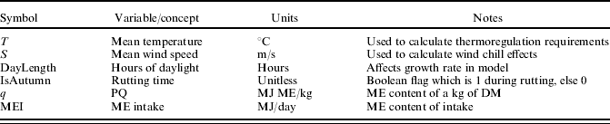
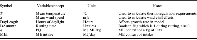
The model described in the current paper was developed as a module for ‘InverDeer’, an individual-animal-based whole-farm simulation system aimed at predicting venison production in intensive deer farming systems (Rollo et al. Reference Rollo, Stevens, Woodward, Archer, Asher, Vetharaniam, Zerger and Argent2005). These systems are based on forage, with small amounts of grain supplementation, and are dominated by red deer and elk. The model was required to predict, on an individual basis, the feed requirements of farmed deer, and their performance on different planes of nutrition. Required performance predictions included the growth of adult stags and hinds, the gestation lengths and birth weights of calves, the milk production of hinds, and the growth of calves through to maturity. These predictions needed to be sensitive to season, temperature, degree of maturity and to feed intake. Inputs required by the model are presented in Table 1. An energy-based approach was considered appropriate for the systems context in which the model would be used.

Table 1.

External inputs required by the model in order to make predictions, the names or symbols used for these inputs, and their corresponding units

Within the scope of energy-based growth prediction, approaches generally diverge along two lines. The more mechanistic approaches represent synthesis and degradation as separate processes whose difference determines the change in mass (e.g. Koong et al. Reference Koong, Falter and Lucas1982a; Oltjen et al. Reference Oltjen, Bywater, Baldwin and Garret1986; Vetharaniam et al. Reference Vetharaniam, McCall, Fennessy and Garrick2001; Vetharaniam & Davis Reference Vetharaniam, Davis, Kebreab, Dijkstra, Bannink, Gerrits and France2006). The more empirical approaches specify a maintenance requirement and calculate an animal's energy balance based on its energy intake and expenditure (e.g. Devir et al. Reference Devir, Zur, Maltz, Genizi and Antler1995; Finlayson et al. Reference Finlayson, Cacho and Bywater1995). The choice of approach may be influenced by the amount of information and data available, and by other constraints such as user requirements. In the current study, in order to include it in the whole-farm simulation, the deer model had to be implemented using a Visual Basic algorithm, with solution by the Euler method and a daily time step. Although a mechanistic approach is more biologically faithful and dynamic, it would typically result in a set of (sometimes stiff) differential equations requiring solution by more powerful integration techniques (Press et al. Reference Press, Teukolsky, Vetterling and Flannery2002). Thus, the more empirical, energy-balance approach for describing growth was adopted in the current paper, since it is more easily formulated as a set of difference equations.

Values for parameters in the model were obtained from the literature. The performance of the model was tested by comparing its predictions with data for the growth of calves and young deer on ad libitum feeding, and pregnancy data (hind weight gains, gestation lengths and calf birth weights) for three planes of nutrition. Although suitable lactation data were not available for testing lactation predictions, milk production was still simulated for different planes of nutrition and used to predict calf growth rates.

MODEL CONSTRUCTION

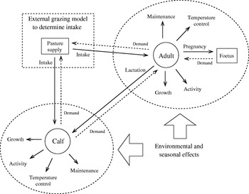
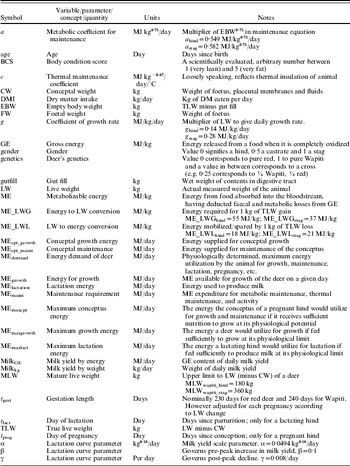
The model linked together a number of empirical functions in a construction that was guided by a combination of data sets and models for other livestock. The construction of the model required some biological and behavioural knowledge, which is not currently available (and may in fact not be measurable), and so several assumptions were needed. For calves, these included models for the post-partum suckling of calves, initiation of calf grazing, the grazing behaviour of suckling calves, relative intakes of milk and pasture under different maternal and pastoral conditions, changes in body water content of calves in the first weeks post-partum, and the activity profiles of calves. Similarly for adults, activity profiles and the relationship between stress and levels of activity were important, but not available. Variables, parameters (with values) and abbreviations used in the model are presented in Table 2. A schema of the model is given in Fig. 1, a brief outline of the model approach is given in the following subsections, and the model equations are presented in the Appendix.

Fig. 1.

Schema showing the energy flows (solid arrows) within the deer model (represented by a dotted oval) for both a hind and a calf. The block arrows indicate that seasonal and environmental inputs are needed by the model (these are listed in Table 1). Dotted arrows indicate demands for energy placed on an animal or food source. An animal's daily demand for pasture is generated by the deer model, and is input into some foraging model of choice. The output from this foraging model (quantity and quality of feed) is then supplied as an input to the deer model. Similarly, milk produced by the hind becomes an input for her calf. A schema for a stag will be similar to that for a hind (minus, of course, the lactation and pregnancy components).

Table 2.

Variables, parameters values and abbreviations used in the deer model, and their explanations

Intake demand

The model used the concept of ‘metabolic demand’ (calculated daily) as a driver of hunger in the deer. This was defined as the maximum daily utilization of metabolizable energy (ME) by a deer, if its energy intake were unconstrained by rumen capacity, satiation or food availability. Calculation of metabolic demand was as follows. First, the maximum possible (energy-unconstrained) growth rate and milk production of a deer were predicted. Metabolic demand was then calculated as the sum of the ME requirements for these maxima, the ME requirements for the metabolic maintenance, thermal regulation and activity of the deer, and the maximum ME consumption of the conceptus.

The metabolic demand is often larger than the ME intake (MEI) of a high-quality, ad libitum diet. Thus, the metabolic demand was moderated by a function reflecting rumen-fill and satiation effects on appetite, to produce an energy-intake demand that the deer would attempt to meet by foraging.

Rumen-fill effects, in addition to reflecting rumen capacity, were also governed by the mean retention time (MRT) of feed. The MRT was predicted as a function of pasture quality (PQ) using a relationship between neutral detergent fibre (NDF) and PQ from Holmes et al. (Reference Holmes, Brookes, Garrick, MacKenzie, Parkinson and Wilson2002), and a relationship between MRT and NDF based on results from Spalinger & Robbins (Reference Spalinger, Robbins and Handley1986), Sibbald & Milne (Reference Sibbald and Milne1993) and Kusmartono et al. (Reference Kusmartono and Barry1997). The MRT was also used to calculate gut fill, based on data from Sibbald & Milne (Reference Sibbald and Milne1993), and thus to estimate empty body weight (EBW) from live weight (LW).

When the model is run in the context of a whole-farm simulation, this energy intake demand would be supplied to a foraging model such as Q-Graze (Woodward et al. Reference Woodward, Lambert, Litherland and Boom2001) to return a prediction of actual daily MEI, which can then be ‘fed’ back to the deer. When the model is operated in a stand-alone fashion to test predictions of trials, pre-specified MEI values would be used instead. The ratio of MEI to ME demand, referred to as the ‘energy status’ (ES) of the deer is used to determine milk production and conceptus growth, using an ‘elasticity of energy supply’ approach (Vetharaniam et al. Reference Vetharaniam, McCall, Fennessy and Garrick2001).

Performance during lactation

A hind's maximum daily milk yield, in kg, was expressed by taking the equation of Wood (Reference Wood1967) and multiplying it by hind EBW^0·84. The latter step was based on published relationships between milk yield and animal size (Linzell Reference Linzell1972). Landete-Castillejos et al. (Reference Landete-Castillejos, Garcia, Gómez, Molina and Gallego2003) found that milk production was related to hind LW^0·77, although their comparison was over a much narrower range of hind genotype and LW than the range of red deer genotypes in New Zealand that this model was intended to emulate. The maximum milk yield curve was calibrated to data for red deer fed rye grass from Loudon & Kay (Reference Loudon, Kay, Peaker, Vernon and Knight1984). The parameters used produced a peak lactation value of 2·09 kg milk/day for a hind with an EBW of 100 kg hind. This lactation yield is similar to the peak lactations found in Iberian red deer Cervus elaphus hispanicus (Garcia et al. Reference Garcia, Landete-Castillejos, Molina, Albinana, Fernandez, Garde and Gallego1999; Landete-Castillejos & Gallego Reference Landete-Castillejos and Gallego2000; Landete-Castillejos et al. Reference Landete-Castillejos, Garcia, Garde and Gallego2000) and in data on New Zealand red deer (Ward et al. Reference Ward, Archer, Asher, Barrell and Littlejohn2008).

Recent, more physiologically based, models of lactation are available (e.g. Vetharaniam et al. Reference Vetharaniam, Davis, Upsdell, Kolver and Pleasants2003) but have more parameters to fit than Wood's equation (Wood Reference Wood1967), which suffices for this problem. Prediction of the ME required for maximum daily milk production assumed an energy content of milk based on data from Arman et al. (Reference Arman, Kay, Goodall and Sharman1974), and an efficiency of milk synthesis of 0·63 (Holmes et al. Reference Holmes, Brookes, Garrick, MacKenzie, Parkinson and Wilson2002). Daily milk production was predicted by multiplying the maximum daily production by the deer's ES raised to the power of a ‘lactation elasticity’ parameter.

Conceptus and foetal growth during pregnancy

The maximum energy consumption of the conceptus was defined as the energy for maximum conceptus growth plus energy required for conceptus maintenance. The maximum rate of conceptus growth was expressed as a function of stage of pregnancy and conceptus weight (CW) and calibrated to conceptus growth curves (assumed to be maximal) from a pregnancy trial performed by Adam et al. (Reference Adam, McDonald, Moir and Pennie1988a). The energy content of the conceptus was expressed as a function of stage of pregnancy, based on results from Adam et al. (Reference Adam, McDonald, Moir and Smart1988b). These two curves were multiplied to give the maximum rate of energy accretion by the conceptus, and then divided by the conceptus’ efficiency of deposition of energy as tissue (ARC 1980) to give the energy for maximum conceptus growth. Conceptus maintenance was assumed proportional to CW raised to the power of 0·75. Energy supplied to the conceptus was predicted by multiplying the maximum energy consumption of the conceptus by the ES raised to the power of a conceptus elasticity parameter. Subtracting conceptus maintenance requirements from this gave the energy available for conceptus growth. Adjusting for conceptus energy density, and for efficiency of energy deposition as tissue, gave the daily growth of the conceptus. Foetal weight (FW) at any time was obtained using an empirical relationship between FW and CW based on data from Adam et al. (Reference Adam, McDonald, Moir and Pennie1988a).

Requirements for maintenance, temperature regulation and activity

Metabolic maintenance requirements were calculated proportional to EBW^0·75, with the coefficient of proportionality varying with age of the deer. ME required for temperature regulation was evaluated as a function of the deer's body condition score (BCS), its surface area (estimated from its EBW) and wind-chill temperature (calculated from mean temperature and wind speed using a formula given by Siple & Passel Reference Siple and Passel1945). ME expenditure for activity was calculated as a function of LW and age of the deer, with the assumption that new-born calves had negligible activity, which steadily increased to adult levels after about 6 weeks. ME for metabolic maintenance, thermal regulation and activity were added together to form a ‘maintenance requirement’.

Growth rates

The maximum growth rate (predicted to occur if the deer received maximal nutrition) was calculated using the same equation for both hinds and stags, with differences between the sexes being implemented via a growth parameter. For the first 9 months of life, hinds and stags have the same relative growth rate (Suttie et al. Reference Suttie, Fennessy, VeenVliet, Littlejohn, Fisher, Corson and Labes1987) and thus had the same value for the growth parameter during this period. Otherwise the growth parameter was higher for stags, except during the rut, when it was set to zero. Increasing photoperiod increases growth rates in deer (Webster et al. Reference Webster, Corson, Littlejohn and Suttie1997) and this was reflected in the maximum-growth-rate function. Additionally, a decrease in growth rate with age was implemented to improve model behaviour. Prediction of LW change was not performed using an elasticity of energy supply approach, but rather using an energy balance approach. Predicted ME used for metabolic maintenance, thermal regulation, activity, lactation and pregnancy was subtracted from daily MEI, resulting in a positive or negative energy balance and thus a prediction of, respectively, a gain or loss of weight. Energy–weight conversion rates differed for a positive or negative energy balance, but were otherwise fixed, and did not reflect changes in body composition, except for young calves, where an increase in water content of lean tissue was hypothesized in order to improve the fit.

Gestation length

Gestation length varies with hind nutrition, with hinds experiencing greater weight gain in the last trimester of pregnancy having a shorter term (Asher et al. Reference Asher, Mulley, O'Neill, Scott, Jopson and Littlejohn2005). This was implemented in the model by altering the gestation period proportionally to a pregnant hind's change in LW between day 150 and day 220 of pregnancy.

BCS

A deer's BCS was used to calculate the lower limit of its thermo-neutral region. Since BCS is a subjective measure, its prediction from LW is arguably problematic. The approach taken in the model was to synthesize a standard LW growth curve against age which corresponds to a BCS of 3 (on a 1–5 scale; Audige et al. Reference Audigé, Wilson and Morris1998). A function was then used to relate deviations in LW from the standard curve to a nominal BCS.

MODEL PREDICTIONS FOR RED DEER

Growth of young deer

The model was used to simulate a trial presented by Suttie et al. (Reference Suttie, Fennessy, VeenVliet, Littlejohn, Fisher, Corson and Labes1987) in which young hinds and stags aged 152 days were grown to 517 days old. The weekly allowances given in that trial were adapted to daily intakes to be input into the model and then adjusted upwards by an amount equal to the daily energy expenditure assumed in the model: the deer in the Suttie et al. (Reference Suttie, Fennessy, VeenVliet, Littlejohn, Fisher, Corson and Labes1987) trial were penned and had little exercise requirements.

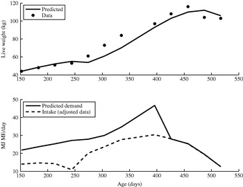
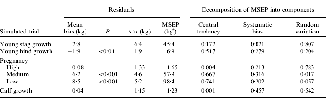
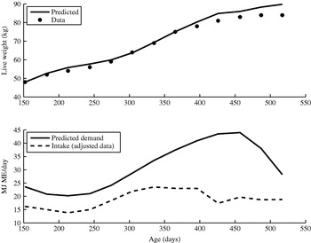
The model simulations of the trial predicted that the stags that weighed 44 kg when 152 days old would reach a weight of 106 kg when 517 days old, compared with the trial average of 103 kg (Fig. 2). However, although model predictions for ages up to 244 days were in close agreement with data, the model under-predicted stag weight for ages 274–457 days, although the error was small except for the ages 304 and 335 days with respective relative errors of 0·17 and 0·16. Model predictions for maximum intake (demand in MJ ME/day) were higher than the adjusted trial allowances, up to about age 425 days, after which there was close agreement between predicted and actual intake. The mean bias for this prediction was not significantly different from zero, and decomposition of the mean square error of the prediction (MSEP) attributed most of the error to random variation (Table 3).

Fig. 2.

Model predictions of young stag growth compared with data from Suttie et al. (Reference Suttie, Fennessy, VeenVliet, Littlejohn, Fisher, Corson and Labes1987), and MEIs supplied to the animal compared with its maximum MEI. Intake data given by Suttie et al. (Reference Suttie, Fennessy, VeenVliet, Littlejohn, Fisher, Corson and Labes1987) for penned deer were incremented by the exercise energy requirements of free-roaming deer to provide the adjusted intake curve shown in the bottom graph. Table 3 gives model performance statistics for this trial.

Table 3.

Model performance in predicting LW during simulations of the following trials: young stag and hind growth, pregnant hinds on high, medium and low planes of nutrition, and young calf growth. Statistics shown are mean bias (residual mean), standard deviation (s.d.) of residuals, MSEP and the decomposition of MSEP into central tendency, systematic bias and random variation components. Tedeschi (Reference Tedeschi2006) gives a discussion of this decomposition

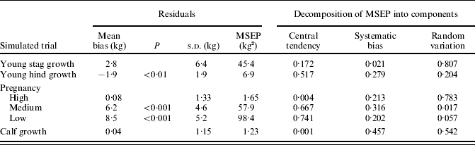
For hinds, the model predicted that 48 kg hinds, aged 152 days, would grow to 90 kg at 517 days old, compared with a trial average of 84 kg. Model predictions for LW appeared to be in close agreement with data (Fig. 3), with a relative error at the end of this simulation of only 0·07. However, the model started to increasingly over-predict LW for ages 396–517 days, with the mean bias in this prediction (−1·9) being significantly different from zero (P<0·01), and 0·52 by proportion of the MSEP being attributable to central tendency. Predicted maximum intake was consistently higher than the trial allowance, and for age 426 days was 1·5 times higher. Results for hinds are graphed in Fig. 3 and model performance summarized in Table 3.

Fig. 3.

Model predictions of young hind growth compared with data from Suttie et al. (Reference Suttie, Fennessy, VeenVliet, Littlejohn, Fisher, Corson and Labes1987), and MEIs supplied to the animal compared with its maximum MEI. Intake data given by Suttie et al. (Reference Suttie, Fennessy, VeenVliet, Littlejohn, Fisher, Corson and Labes1987) for penned deer were incremented by the exercise energy requirements of free-roaming deer to provide the adjusted intake curve shown in the bottom graph. Table 3 gives model performance statistics for this trial.

Pregnancy under different nutritional planes

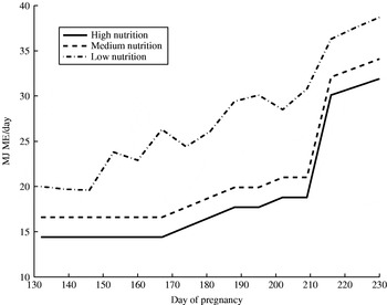
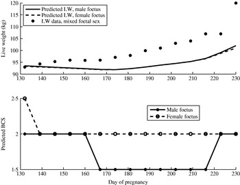
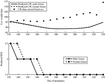
The model was then used to simulate results from trials with pregnant hinds under three planes of nutrition, using the ME values (Fig. 4) as reported by Asher et al. (Reference Asher, Mulley, O'Neill, Scott, Jopson and Littlejohn2005). For each nutrition plane, the model was started with a hind of LW 90 kg at age 518 days, i.e. continuing on from the end point of the simulation of the Suttie et al. (Reference Suttie, Fennessy, VeenVliet, Littlejohn, Fisher, Corson and Labes1987) trial. Data were not available for the first 131 days of pregnancy (Asher et al. Reference Asher, Mulley, O'Neill, Scott, Jopson and Littlejohn2005), and so hinds on each nutritional plane were fed 17 MJ of ME per day for that period, following Adam et al. (Reference Adam, McDonald, Moir and Pennie1988a). From day 132 to day 213 of pregnancy, a feed allowance was given based on data from Asher et al. (Reference Asher, Mulley, O'Neill, Scott, Jopson and Littlejohn2005). From day 214 till the end of pregnancy, the hinds were fed ad libitum (Asher et al. Reference Asher, Mulley, O'Neill, Scott, Jopson and Littlejohn2005), with their MEI being set at predicted demand.

Fig. 4.

MEIs for hinds under three different nutritional levels (low, medium and high) used to simulate outputs in Figs 5–7.

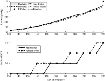
For the high nutrition hinds, simulated and actual hind LW compared well (Fig. 5). However, simulated hind LW for the medium and low nutrition trials were well below what was actually measured (Figs 6 and 7). Residual means for the high, medium and low nutritional planes were, respectively, 0·08, 6·2 and 8·5 kg, with standard deviations of 1·33, 4·6 and 5·2 kg. For the medium and low nutrition trials, the residual means were significantly different from zero (P<0·001). Random variation contributed to 0·78 of the MSEP for the high nutrition trial, while, by contrast, the bulk of the MSEP for the medium and low groups was due to errors in central tendency (respectively, 0·67 and 0·74 by proportion). Table 3 summarizes these and other statistics. Simulated BCS changes for the high nutrition group were also similar to those measured but were much higher for the simulated medium and low nutrition groups.

Fig. 5.

Model predictions of LW and BCS for a pregnant hind under a ‘high’ nutrition regime, compared with data for LW from Asher et al. (Reference Asher, Mulley, O'Neill, Scott, Jopson and Littlejohn2005). Table 3 gives model performance statistics for this trial.

Fig. 6.

Model predictions of LW and BCS for a pregnant hind under a ‘medium’ nutrition regime, compared with data for LW from Asher et al. (Reference Asher, Mulley, O'Neill, Scott, Jopson and Littlejohn2005). Table 3 gives model performance statistics for this trial.

Fig. 7.

Model predictions of LW and BCS for a pregnant hind under a ‘low’ nutrition regime, compared with data for LW from Asher et al. (Reference Asher, Mulley, O'Neill, Scott, Jopson and Littlejohn2005). Table 3 gives model performance statistics for this trial.

Model predictions for gestation length and calf birth weight compared well with the corresponding experimental data for the high nutrition group, but less favourably with the medium and low nutrition groups. Averaged over male and female calves, the model predicted gestation lengths of 231·5, 238 and 242 days for the high, medium and low nutritional plane groups, respectively. Calf gender had no effect on predicted gestation length for the medium and low groups, and was only one day longer for female than male calves for the high group. Experimental averages for gestation lengths were 231·3, 234·7 and 239·2 days for the high, medium and low groups, respectively (Asher et al. Reference Asher, Mulley, O'Neill, Scott, Jopson and Littlejohn2005). Predicted birth weights for stag and hind calves were, respectively, 9·2 and 7·7 kg for the high nutrition group, 9·0 and 7·6 for the medium nutrition group, and 9·7 and 8·2 kg for the low nutrition group. Predicted birth weights averaged over sex were 8·5, 8·3 and 8·9 kg, compared with recorded mixed sex birth weights of 8·4, 9·5 and 9·3 kg for the high, medium and low nutrition groups, respectively (Asher et al. Reference Asher, Mulley, O'Neill, Scott, Jopson and Littlejohn2005). While predictions and experiment agree for the high nutrition group, and were close (0·4 kg) for the low nutrition group, they diverged by 1·1 kg for medium nutrition. Birth weights of mixed sex calves usually range between 8·5 and 9·5 kg, with hind calves having a lower birth weight than stag calves, but by only 0·6 kg (Asher & Adams Reference Asher, Adams, Fennessy and Drew1985). Thus, the simulated differences that averaged 1·5 kg across the nutrition groups are unacceptably high.

Growth of young calves

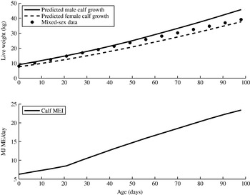
The model was then used to simulate a calf rearing trial performed by G. W. Asher (unpublished data). In that trial, quantities of milk consumed for the first 100 days post-partum had been measured, but forage dry matter (DM) intakes (DMIs) had not. For simulation purposes, it was assumed that, in the first 3 weeks post-partum, calves ate no forage. From day 21 onwards, they were assumed to increase their forage DMI by almost 19 g per day, resulting in a DMI of 1·5 kg after 100 days. Simulations for the trial used initial calf weights equal to the predicted birth weights from the medium nutrition pregnancy simulation, and predicted that male calves would grow from 9·0 to 45·7 kg in the first 98 days of their life, while female calves would grow from 7·6 to 37·6 kg. Trial data averaged across calves showed a growth from 8·3 to 41·7 kg over this time (G. W. Asher, unpublished data). Figure 8 shows the model MEI and comparisons between model predictions for the growth of male and female calves compared with the trial data (averaged across male and female calves). Averaging the predictions for male and female calves, and comparing them with the data yielded a residual mean that was not significantly different from zero, with random error and systematic bias contributing, respectively, 0·54 and 0·46 by proportion to the MSEP (see Table 3).

Fig. 8.

Model predictions for LWs of male and female calves in their first 98 days of life, compared with an actual trial (G. W. Asher, unpublished data), and the average of male and female calf MEIs used as inputs to the model; intakes for males and females differed by less than 2% and so were not shown separately. Table 3 gives model performance statistics for this trial.

Although the male and female calves got the same intake in the simulation, the males grew faster than the females because of a greater efficiency in converting energy to LW.

Lactation

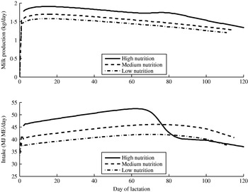
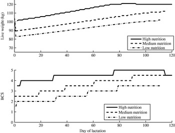
The model was used to predict performance during lactation under ad libitum conditions. This simulation continued on from the end of the simulation of Asher et al. (Reference Asher, Mulley, O'Neill, Scott, Jopson and Littlejohn2005) pregnancy trials. Hinds corresponding to the high, medium and low nutritional planes were continued to be labelled as such in Fig. 9, which show MEI and milk yield, and Fig. 10, which shows LW and BCS. The hinds were fed their ME demand (maximal feeding). The size differences between hinds on different nutritional regimes were significant at the end of the pregnancy simulation, and thus the model predicted differences in maximum milk yields (since these are linked to EBW). This resulted in differences in ME demand, and hence differences in intake and milk yield for the three treatments (Fig. 9). However, simulated growth rates for the hinds were similar in the first half of their lactation since all their energy requirements for growth and lactation were met. The high-nutrition hind reached her maximum LW during the lactation and consequently her intake demand dropped. No data were available for comparison of model prediction with experiment, but these results seem reasonable.

Fig. 9.

Model predictions of milk yield for the different nutritional levels, and the MEIs used in the simulation.

Fig. 10.

Model predictions of LW and BCS for the different nutritional levels shown in Fig. 4.

DISCUSSION

During model construction, the data used for young calves showed greater increases in LW than expected from their intakes. While it is possible that these calves had very high efficiencies in the deposition of ME as tissue, it is more likely that this increased gain in LW was due to increased water content in lean tissue, which is not addressed directly in this energy-based model. Thus for better model prediction it was found necessary to increment LW by a purely empirical ‘re-hydration factor’ (given in Eqn (34) of the Appendix). Experiments investigating the efficiency of tissue deposition in young calves, and the composition of their lean tissue may resolve the uncertainty behind the unexplained weight gain.

In the simulations of pregnancy, for all three nutritional planes simulated, the model failed to capture the rapid increase in LW seen close to term in the actual trial. It is unclear whether this increase is due to a failure of the model to account for a rapid increase in FW or because of fluid accumulation in hinds in the actual trial (and not addressed in the model that is energy based). Figures 5–7 record an unexpectedly large change in hind LW between days 222 and 230 of pregnancy, in the order of 1·25–2 kg/day for hinds on various planes of nutrition during late pregnancy (Asher et al. Reference Asher, Mulley, O'Neill, Scott, Jopson and Littlejohn2005). While it would be expected that hind LW gain would be greatest during the last week of pregnancy (due to the exponential growth of the conceptus, rapid mammary gland extension, and possibly increased water retention by the hind), there is also a potential measurement error in the LW recorded on day 222. For all treatment groups, and especially low and medium nutrition, the LW recorded on day 222 are lower than expected, falling up to 5 kg below the clear curvilinear trend line between days 200 and 230 of pregnancy. The source of this error is unknown, but could relate to proximate biological factors that temporarily influenced gut fill and body hydration leading up to weight recording. This would clearly exaggerate apparent LW gains within the last week of pregnancy. By eliminating the LW readings for day 222 and interpolating from the trend, it is estimated that the actual LW gain in hinds within the last week of pregnancy was around 600–800 g/day, at least half of which was change in total conceptus mass.

The similar predictions for LW and BCS between the medium and low nutrition groups in those simulations reflect the similarity of the MEIs provided to these groups. The model's poor performance in predicting hind LW during pregnancy for these two groups, despite good predictions for the high nutrition group, is likely due to overestimation of both whole-body energy density and maintenance requirements for the lower intakes. The conversion factors for converting ME to (from) kg of LW when a deer is in positive (negative) energy balance assumed a constant body composition. However, Asher et al. (Reference Asher, Mulley, O'Neill, Scott, Jopson and Littlejohn2005) found that pregnant hinds on the low and medium planes of nutrition in their trial had less than half the fat content of hinds on a high nutritional plane, 10 weeks after the imposition of different nutritional regimes. Furthermore, the model specified the same maintenance requirements for any nutritional plane, whereas a reduced requirement for maintenance of the digestive tract may have occurred with the lower feed intakes (Koong et al. Reference Koong, Nienaber, Pekas and Yen1982b; Reference Koong, Ferrell and Nienaber1985). Since gestation period and thus foetal growth in the model are governed by the change in hind LW between days 150 and 220, the discrepancies in gestation period and calf birth weight for the medium and low nutrition groups are likely a result of the poor performance of the model in predicting hind LW. Addressing these deficiencies in the model would have required the adjustment of maintenance requirements and energy-tissue conversion factors with level of intake and BCS. However, insufficient information was available to do this.

The model's predictions on lactation could not be assessed since there were no suitable data. Since a hind's lactation performance is vital for calf growth, gathering such data would be invaluable for the prediction of hind lactation and its responsiveness to nutrition.

The construction of the model was weighted more towards an empirical approach than a mechanistic approach and rather than being fitted to the data used to gauge model performance, the parameters were calibrated on values published in the literature. Much of the data in the literature corresponds to animals on high nutritional planes and thus it could be expected that the model would better predict the response of deer on high-nutrition diets than on medium- or low-nutrition diets, especially since empirical models often predict poorly outside the conditions to which they are calibrated. A more mechanistic approach incorporating synthesis and degradation as intake-dependent functions and dynamically varying energy density of the whole body (e.g. Vetharaniam & Davis Reference Vetharaniam, Davis, Kebreab, Dijkstra, Bannink, Gerrits and France2006) may have provided more robust predictions. For example, Keller (Reference Keller1989) found that of models parameterized to the same data set, the mechanistic model outperformed the empirical one in predicting independent data sets. Of course the success of a mechanistic approach depends on how well it captures the dynamics of the system. Yamashita & Hashida (Reference Yamashita and Hashida2003) observed that when the mechanics of a system are not well understood, empirical models may provide superior performance (albeit providing less insight). The merits of mechanistic v. empirical modelling in energy metabolism have been discussed much earlier by McCracken (Reference McCracken1992). Re-evaluating this issue again is outside the scope of this paper. In passing, however, it is noted that McCracken (Reference McCracken1992) equated mechanistic with a complete knowledge of the system coupled with sufficient biochemical, biophysical and metabolic data to parameterize all equations. A less stringent definition of mechanistic has been employed, which is more compatible with the philosophy espoused by Nestorov et al. (Reference Nestorov, Rowland, Hadjitodorov and Petrov1999) that the empirical-mechanistic distinction is never an absolute one, but rather context based.

CONCLUSION

A research model has been constructed that incorporates a number of measurements from the literature to predict performance over the whole life cycle of a deer. It is easily compared with data and provided good predictions of the performance of deer on a high nutritional plane. However, the model included limited mechanisms for the growth of deer and foetuses, and this perhaps impaired its ability to predict for conditions with sub-optimal nutrition.

The main benefit of the model has been the development process of conceptualizing information and re-examining data to obtain parameter values. This highlighted several gaps in knowledge and was useful in suggesting new experiments to fill these gaps, giving significant insights into research requirements. New research in the lactation and early growth of deer has been developed from the present work and is currently in progress.

We thank M. Upsdell for helpful discussions and J. M. Suttie for making available data used in the paper by Suttie et al. (Reference Suttie, Fennessy, VeenVliet, Littlejohn, Fisher, Corson and Labes1987). This work was funded by a grant from the New Zealand Foundation for Research, Science and Technology.

APPENDIX MODEL DEVELOPMENT

Experimental measurements for deer are usually specified in terms of LW, which is the EBW plus the digesta (and also the weight of the conceptus in the case of a pregnant hind). Because of this, some of the equations in the model are specified in terms of LW, whereas others are specified in terms of EBW. However, in equations relating to pregnant hinds, a third measure of weight is more suitable, ‘true live weight’ (TLW), which we define as LW minus CW:

(1)

${\rm TLW} \equals {\rm LW} \minus {\rm CW}$

EBW was calculated from TLW by estimating gut fill and subtracting this from TLW:

(2)

${\mathss EBW} \equals {\mathss TLW} \minus {\mathss GutFill}$

The formula for estimating GutFill is given by Eqn (28) below.

Metabolic demand

The model is driven by daily intake, which is both a function of animal demand and feed availability. Following (Vetharaniam & Davis Reference Vetharaniam, Davis, Kebreab, Dijkstra, Bannink, Gerrits and France2006), the maximum energy use by the animal for a number of different uses is estimated and used to calculate a ‘metabolic demand’ (Q) in terms of ME, which is used to drive intake:

(3)

$\eqalign{Q \equals \tab {\mathss MaxME{\curr{\uscore}}Growth} \plus {\mathss MaxME\uscoreLact} \cr \tab \plus {\mathss MaxME\uscore Cpt} \plus {\mathss ME\uscore Maint}}$

where MaxME_Growth is the maximum ME the deer can use for growth, MaxME_Lact is the maximum ME deer can use in lactation, MaxME_Cpt is the maximum ME the conceptus can use for growth and ME_Maint is the energy requirement for maintenance.

Maximum growth rate

The maximum growth rate is the growth rate that will be seen if the deer are fed maximally. The same equation was used to calculate the maximum growth rate for both stags and hinds. Stags and hinds experience a difference in growth rate after 9 months of age, and this difference appears in a parameter g (MJ/d), which also incorporates the effect of the autumn rut on stags. The form for the maximum growth equation is

(4)

$\eqalign{\tab{\mathss MaxME\uscore Growth} \equals\cr\tab\quad \left\{ {\matrix{ {g \times {{{\mathss DayLength}} \over {12}} \times {\mathss AgeFactor} \times {\mathss LW\comma }} \hfill \tab {{\mathss LW\ } \lt {\mathss \ MLW}} \hfill \cr {0\comma } \hfill \tab {{\mathss LW\ }\ges {\mathss \ MLW}} \hfill \cr} } \right.$

where the growth factor, g, for hinds is

(5)

$g \equals g_{{\rm hind}}$

and for stags is

(6)

$g \equals \left\{ {\matrix{ {g_{{\rm hind}} } \hfill \tab {{\mathss age} \lt {\rm 270 \ d}} \hfill \cr {g_{{\rm stag}} \times \left( {1 \minus {\mathss IsAutumn}} \right)} \hfill \tab {{\mathss else}} \hfill \cr} } \right.$

Growth of deer exposed to longer day lengths is higher than that for deer exposed to shorter day lengths (Webster et al. Reference Webster, Corson, Littlejohn and Suttie1997). In Eqn (4) day length is assumed to have a positive linear effect on the maximum growth rate of the deer, and this will have an indirect flow-on effect on actual growth rate. The factor IsAutumn is set outside the model, to stop growth during the breeding season (the rut) as stags reduce their intake. The function AgeFactor slows down growth rates with age and was introduced to improve the behaviour of the model:

(7)

$\hskip-3\eqalign{{\mathss AgeFactor} \equals \tab 10 \times {\mathss exp}\lpar\! \minus 0.02 \times {\mathss age}\rpar \cr \tab \plus \lpar 0.5 \plus 2\sol \lpar 1 \plus {\mathss exp}\lpar\! \minus 0.03 \!\times\! \lpar 500 \hskip-1\minus\hskip-1 {\mathss age}\rpar \rpar \rpar \rpar }$

Maximum milk production

It is assumed that milk production has an efficiency of 0·63 (Holmes et al. Reference Holmes, Brookes, Garrick, MacKenzie, Parkinson and Wilson2002). This means that the actual cost of producing milk is 1·59 times the gross energy (GE) content of the milk. Therefore the maximum daily energy usage of a lactating hind is

(8)

${\mathss MaxME\uscore Lact } \equals {1{\cdot}59} \times {\mathss MaxGE\uscore Milk}$

where MaxGE_Milk is the GE content, GE_ContentMilk (MJ/kg), of a hind's maximum milk production, Max_kgMilk (kg):

(9)

${\mathss MaxGE}\uscore {\mathss Milk} \equals {\mathss \ Max\uscore kgMilk \lowast GE\uscore ContentMilk}$

The maximum milk yield (in kg) from a hind was expressed using a modification of Wood's equation (Wood Reference Wood1967):

(10)

${\mathss Max\uscore kgMilk} \equals \rmalpha \times t^{\rmbeta } {\mathss exp\lpar\! \minus }\rmgamma t_{\rm lact} \rpar \times {\mathss EBW}^{\setnum{0 {\cdot} 84}}$

where α, β and γ are Wood's equation parameters (Wood Reference Wood1967), which need to be estimated from data, t _lact is the day of lactation, and the factor EBW^0·84 governs the relationship between milk yield and animal size, based on results from (Linzell Reference Linzell1972) who found a 0·84 power relationship between LW and milk yield. Values for the parameters in Eqn (10) were obtained by calibrating the curve to data for red deer on rye grass (Loudon & Kay Reference Loudon, Kay, Peaker, Vernon and Knight1984). These are shown in Table 2. The GE content of milk, GE_ContentMilk, was specified in units of MJ/kg, and was calculated using the following expression that interpolates data from Arman et al. (Reference Arman, Kay, Goodall and Sharman1974) :

(11)

$\scale93%\eqalign{\tab{\mathss GE\uscore ContentMilk} \equals\cr\tab \!\left\{\! {\matrix{ {1 {\cdot}425 \hskip-1\times\hskip-1 10^{ \minus \setnum{4}} t_{{\rm lact}} ^{\hskip11\setnum{2}} \!\plus \!1{\cdot}06 \hskip-1\times\hskip-1 10^{ \minus \setnum{2}} t_{{\rm lact}} \plus 5{\cdot}2461} \hfill \tab\! {0\les t_{{\rm lact}} \les 101} \hfill \cr {7{\cdot}77} \hfill \tab\! {t_{{\rm lact}} \gt 101} \hfill \cr} } \right.$

where t _lact is the day of lactation.

Maximum conceptus growth

The maximum energy that can be used by the conceptus on any day, MaxME_Cpt, is the sum of the conceptus' maintenance requirement, and the maximum energy for conceptal growth, calculated from MaxConceptusGrowth for that day and the energy content of the foetus, EnergyContentConceptus, for the next day:

(12)

$\eqalign {\tab\hskip-14pt {\mathss MaxME\uscore Cpt}\left( {t_{{\rm preg}} } \right) \equals {\mathss MaxConceptusGrowth\lpar }t_{{\rm preg}} {\rpar }\cr\tab\times {\mathss EnergyContentConceptus\lpar }t_{{\rm preg}} \plus {1\rpar \sol 0 {\cdot}133} \cr \tab \plus {\mathss ME\uscore ConceptusMaint} \cr}$

where t _preg is the day of pregnancy. The factor 0·133 in the above equation is the efficiency of the conceptus at utilizing energy for growth (ARC 1980). The energy content of the conceptus for the next day is used instead of that for the current day to reflect a change in tissue composition.

Maintenance requirements for the conceptus are estimated by the formula

(13)

${\mathss ME\uscore ConceptusMaint} \equals 0{\cdot}26 \times {\mathss CW}^{{\rm \setnum{0{\cdot}75}}}$

MaxConceptusGrowth is assumed to depend on the weight of the conceptus and the stage of pregnancy:

(14)

$\eqalign{\tab{\mathss MaxConceptusGrowth} \equals\big\{ \!\exp \lpar {8{\cdot}248\right}\cr\tab\times\big[ {1 \!\minus\! \exp \lpar\! \minus 0{\cdot}01138\rpar } \right]\exp \lpar\! \minus 0{\cdot}01138t_{{\rm preg}} \rpar \rpar\! \minus\! 1 \big\} \times {\mathss CW}$

(The coefficients in the above equation have been calibrated by fitting to data presented by Adam et al. (Reference Adam, McDonald, Moir and Smart1988b), under the assumption that the conceptuses in that trial were growing at a maximum rate.)

The energy content of the conceptus in MJ/kg is given by the following equation calibrated using data from Adam et al. (Reference Adam, McDonald, Moir and Pennie1988a):

(15)

$\eqalign{\tab\hskip-14pt{\mathss EnergyContentConceptus\lpar t\rpar } \equals\hfill\cr\tab{\rm 6{\cdot}68} \times {\rm 10}^{ \minus {\rm \setnum{1}}} \plus {\rm 9{\cdot}18 \times {\rm 10}^{ \minus {\rm \setnum{3}}} {\it t}_{{\rm preg}}} \plus {{\rm 3{\cdot}93} \times {\rm 10}^{ \minus {\rm \setnum{5}}} t_{{\rm preg}} ^{\hskip10\setnum{2}}}\hfill$

Maintenance requirements

ME_Maint includes energy for thermal maintenance and activity and is given by

(16)

$\eqalign{{\mathss ME\uscore maint} \equals \tab a \times \lpar 1 \plus b\rpar \times {\mathss EBW}^{\setnum{0{\cdot}75}} \plus {\mathss HeatLoss} \cr \tab \plus {\mathss ExerciseEnergy}}$

where the first term corresponds to metabolic maintenance requirements. The maintenance coefficient, a (units of MJ kg^−0·75), varies between stags and hinds, and is increased by 10% for pregnant hinds. b (unitless) is a function of age designed to increase the maintenance coefficient for calves by 10% at birth, with a linear decline to an adult value at 150 days:

(17)

$b \equals 0{\cdot}1 \minus \min \lpar {\mathss age\comma 150\rpar \sol 1500}$

In developing the HeatLoss function it was assumed that the temperature at which a deer goes below its thermoneutral zone (and needs to generate extra energy to keep warm) increases as BCS decreases. As the temperature decreases below this cut-off temperature, this energy requirement increases linearly with decrease in temperature:

(18)

$\eqalign{{\mathss HeatLoss} \equals \tab \max \lpar 20 \minus 3 \times {\mathss BCS} \minus T_{{\rm eff\, }} \comma 0\rpar \cr \tab\times c \times 0{\cdot}09 \times {\mathss EBW}^{\setnum{0}\cdot\setnum{67}}}$

where T _eff is the effective environmental temperature, incorporating wind chill effects. The value of 0·09×EBW^0·67 gives the surface area of the deer, and c reflects the thermal insulation of the deer. EBW was used instead of LW since LW can change considerably with intake while surface area will not be so largely affected. EBW is calculated from LW and intake – see Eqn (2). T _eff is evaluated using the (Siple & Passel Reference Siple and Passel1945) formula:

(19)

$\scale90%\eqalign{\tab T_{{\rm eff}} \equals\cr\tab \!\!\left\{\! {\matrix{ {{\rm 33} \plus {\rm \lpar }T \minus {\rm 33\rpar }\hskip-1 \times\hskip-1 {\rm \lpar 0{\cdot}474} \plus {\rm 0{\cdot}454\ }\sqrt S \minus 0{\rm {\cdot}0454\ }S{\rm \rpar \comma }} \hfill \tab\hskip-4 {S \gt 1{\cdot}8{\rm \ m\sol s}} \hfill \cr {T\comma } \hfill \tab\hskip-4 {{\rm else}} \hfill \cr} } \right.$

where T is the mean daily temperature (Celsius) and S is mean daily wind speed in metres per second.

At birth, red deer calves are largely sedentary for a number of days, and then gradually increase their activity. There is little published information on the nature of this transition or of the quantification of energy expenditure, and thus a number of assumptions must be made regarding the amount of activity at any age, and the cost of that activity. It was assumed that calves up to 14 days old have negligible activity requirements, that from age 15 days to 6 weeks the distance they travel increases with age to 3 km/day and that after 6 weeks of age they maintain a travelling distance of 3 km/day. The cost of travel (walking) was assumed to be 0·0026 MJ/kg of LW/km travelled and the daily cost of standing was assumed to be 0·01 MJ/kg of LW/day based on results from AAC (1990). The following equation resulted:

(20)

$\scale91%\eqalign{\tab{\mathss ExerciseEnergy} \equals\cr\tab \!\left\{\!\! {\matrix{ 0 \tab {{\mathss age}\les {\mathss 14\ days}} \cr {\lpar {\mathss age} \minus 14\rpar \sol 28 \times \lpar 0{\cdot}01 \plus 3 \times 0{\cdot}0026\rpar \times {\mathss LW}} \tab {15\les {\mathss age}\les 42} \cr {\lpar 0{\cdot}01 \plus 3 \times 0{\cdot}0026\rpar \times {\mathss LW}} \tab {{\mathss else}} \cr} } \right.$

Determining actual performance

The actual performance of the animal is determined by its intake, which is influenced by the animal's appetite and feed availability. The metabolic demand, Q, indicates the capacity of cells for energy expenditure, and the potential of the animal to produce if it were to receive sufficient nutrition. However, it does not take into account satiation effects or rumen-fill in limiting intake.

Calculating intake demand

Therefore a function, J (MJ ME/day), indicating the degree of hunger of the animal, was used to predict an MEI demand based on the metabolic demand, Q, absorption capacity and rumen processing capacity:

(21)

$J \equals J_{c} \minus {1 \over k}\log \left( {1 \minus \exp \left[ {\minus kQ} \right]\left\{ {1 \minus \exp \left[ {k\ J_{c} } \right]} \right\}} \right)$

where k (day/MJ ME) is an intake demand regulator and J _c is intake capacity in MJ ME/day, given by

(22)

$J_{c} \equals A_{c} \minus {1 \over c}\log \left( {1 \minus \exp \left(\! { \minus cP_{c} } \right)\left\{ {1 \minus \exp \left[ {cA_{c} } \right]} \right\}} \right)$

where c (day/MJ ME) is an intake capacity regulator, A _c is absorptive capacity (MJ ME/day) given by

(23)

$A_{c} \equals a_{c} \times {EBW}$

where a _c (MJ kg/day) relates EBW to A _c; P _c is the processing capacity of the rumen (MJ ME/day) given by

(24)

$P_{c} \equals q \ \rmrho \rmtheta \ R\ r_{o}$

where q is PQ (MJ ME/kg DM), ρ (kg/l) is the density of rumen wet fill, θ (kg DM/kg) is the DM fraction of rumen wet fill, r _o (/day) is the outflow rate from the rumen and R, in litres, is the rumen capacity, given by

(25)

$R_{c} \equals r_{c} \times {\rm EBW}$

where r _c has units litre/kg/day.

When PQ is low, P _c<A _c, and thus demand is limited by rumen capacity; when PQ is high, P _c<A _c, and thus demand is limited by visceral capacity. Both A _c and P _c can be varied with time to reflect adjustment of the animal to different levels of intake.

The intake demand J is intended as input to a foraging model, external to the deer model, which will in turn predict the daily MEI of the deer:

(26)

${\mathss MEI} \equals G\lpar J\comma \tilde{\rmpsi }\rpar$

where G represents the prediction of the foraging model as a function of J and environmental, physical and behavioural parameters . In simulations, the Q-Graze foraging model (Woodward et al. Reference Woodward, Lambert, Litherland and Boom2001) was used. The daily DMI of the deer is then calculated by the ratio of MEI and PQ:

(27)

${\mathss DMI } \equals {\mathss MEI}\sol {\rm q}$

Calculating gut fill

A deer's gut fill was calculated from its DMI, the daily rate, r _o, at which its feed disappears from the rumen (either through absorption or passage into the abomasum), and the kg of rumen DM per kg of rumen wet matter. To do this, it was assumed that on average, daily rumen DM efflux (given by rumen DM content times r _o) equals DMI, and, that the weight of digesta in the total tract is approximately 1·6 times that in the rumen (Sibbald & Milne Reference Sibbald and Milne1993):

(28)

${\mathss GutFill } \equals {\rm 1{\cdot}6} \times {\mathss DMI \sol }r_{o} {\mathss \sol DM\uscore ContentRumenWetFill}$

Now, r _o is given by MRT in hours by

(29)

$r_{o} {\rm } \equals {\mathss 24 \sol MRT}$

Spalinger & Robbins (Reference Spalinger, Robbins and Handley1986) investigated the rumen MRT of a range of different forages in elk, and found that while mean cell wall thickness (MCWT) was the likely determinant of MRT, both lignin and NDF were positively correlated with MRT due to their positive correlation to MCWT. The quality of feed input into the model was expressed in terms of PQ and using data for pasture from Holmes et al. (Reference Holmes, Brookes, Garrick, MacKenzie, Parkinson and Wilson2002) the DM percentage of NDF was expressed as a function of PQ using the formula

(30)

${\mathss NDF } \equals {\rm \ 123{\cdot}4} \minus 7.286q$

and following Küffer et al. (Reference Küffer, Fischlin and Filli2001), a Spalinger & Robbins (Reference Spalinger, Robbins and Handley1986) regression relating NDF to MRT in elk was used. The data used by Spalinger & Robbins (Reference Spalinger, Robbins and Handley1986) were from a range of forages with NDF values ranging from 110 to 900 g/kg and MRT values ranging from 1·7 to 8·9, but these forages were largely dissimilar to pasture. The literature suggests higher MRT in red deer and elk: 21 h for grass hay (Sibbald & Milne Reference Sibbald and Milne1993); 11·6 h for perennial ryegrass (Kusmartono et al. Reference Kusmartono and Barry1997), and thus a 50 % increase was used over the regression used by Spalinger & Robbins (Reference Spalinger, Robbins and Handley1986) for MRT in hours.

(31)

${\mathss MRT } \equals {\rm 1{\cdot}5} \times {\rm \lpar 2{\cdot}975}\ {\mathss log\ \lpar NDF\rpar } \minus {\rm 3{\cdot}973 \rpar}$

Calculating actual growth rate

The ME associated with growth for each day was calculated using the equation

(32)

$\eqalign{\tab\hskip-8pt{\mathss ME\uscore Growth } \equals {\mathss MEI} \minus {\mathss ME\uscore Maint} \minus{\mathss ME\uscore Lact}\cr\tab \minus {\mathss ME\uscore ConceptusGrowth} \minus {\mathss ME\uscore ConceptusMaint}_{}$

A positive (negative) value for ME_Growth is associated with a gain (loss) in TLW, where TLW is defined as LW minus CW. TLW equals LW except for a pregnant hind. Change in TLW is given by

(33)

$\rmDelta {\mathss TLW } \equals\! \left\{\! {\matrix{ {{\mathss ME\uscore Growth}\sol {\mathss {\mathss M}{\mathss E}}\uscore {\mathss LWL}} \tab {{\mathss ME\uscore Growth\ } \lt 0} \cr {{\mathss ME\uscore Growth}\sol {\mathss {\mathss M}{\mathss E}}\uscore {\mathss LWG}} \tab {{\mathss ME\uscore Growth\ }\ges 0} \cr} } \right.$

where ME_LWL and ME_LWG are the energy content of, respectively, LW loss and LW gain.

In order to better predict the growth of young calves, it was necessary to additionally augment ΔTLW by the following ‘re-hydration’ term, reflecting a hypothesized increase in water retention in lean tissue:

(34)

$\eqalign{\mathss Rehydration} \equals 0 {\cdot}02 \times \exp \lpar\! \minus 0{\cdot}02 \times {\mathss age\rpar } \times {\mathss TLW}$

Calculating actual milk yield

In order to estimate actual milk yield, the concept of elasticity of production is used (Vetharaniam & Davis Reference Vetharaniam, Davis, Kebreab, Dijkstra, Bannink, Gerrits and France2006). MaxGE_Milk is the upper limit of a hind's milk production in MJ of GE, and the hind is assumed to produce this if she is fed maximally (i.e. if MEI=ME_Demand). Otherwise, as MEI is progressively lower than ME_Demand milk production becomes lower at a rate governed by an elasticity parameter, ε. The expression for milk produced is

(35)

${\mathss GE\uscore Milk} \equals {\mathss MaxGE\uscore Milk} \times \left( {{\raise0.7ex\hbox{${{\mathss MEI}}$} \!\mathord{\left/ {\vphantom {{{\mathss MEI}} {{\rm ME\uscore Demand}}}}\right.\kern-\nulldelimiterspace}\!\lower0.7ex\hbox{${{\mathss ME\uscore Demand}}$}}} \right)}^{\rmepsiv }\hfill\hskip-12pt$

In the model, ε is taken as 0·5, which means that if MEI is half of ME_Demand, then GE_Milk will be 0·70 of MaxGE_Milk.

The amount of milk produced is then given by

(36)

${\mathss kgMilk} \equals {\mathss GE\uscore Milk \sol GE\uscore ContentMilk}$

where GE_ContentMilk is given in Eqn (11) and the actual usage is

(37)

${\mathss ME\uscore Lact } \equals {\rm 1{\cdot} 59} \times {\mathss GE\uscore Milk}$

Calculating energy partitioned to pregnancy

Energy partitioned to pregnancy is, like in the case of lactation, governed by an elasticity-of-energy-supply parameter, e, and the ratio of MEI to ME_Demand

(38)

$\scale93%\eqalign{{\mathss ME\uscore Conceptus} \equals \left( {{{{\mathss MEI}} \over {{\mathss ME\uscore Demand}}}} \right)^{e} {\mathss MaxME\uscore Conceptus}$

(39)

$\eqalign{\tab\hskip-26pt{\mathss ME\uscore ConceptusGrowth} \equals\hfill\cr\tab\hskip-6pt {\mathss ME\uscore Conceptus} \minus {\mathss ME\uscore ConceptusMaint}\hfill$

e is currently used with the value 0·1. This small value buffers conceptal growth under low nutrition.

At the start of pregnancy, CW was initialized to 0·00905 kg for a red male foetus, and 0·00762 kg for a red female foetus at the time of conception. For a wapiti foetus, the initial CW is scaled by a factor of 1·5. The actual growth of the conceptus depends on ME_ConceptusGrowth, the energy supplied for conceptual growth, according to the following equation

(40)

$\eqalign{\tab{\rmDelta {\mathss CW} \equals 0.133 \times {\mathss ME\uscore ConceptusGrowth}\sol}\hskip55pt\cr\tab\quad {\mathss EnContentConceptus}\left( {t_{\rm preg} \plus 1} \right)$

where the factor 0·133 is the efficiency of energy deposition as tissue (ARC 1980).

The model calculates growth in CW directly, and estimates FW in kg using an empirical relationship between FW and CW:

(41)

$\eqalign{{\mathss FW} \equals \tab \left( {0{\cdot}311 \minus 0{\cdot}0107t_{{\rm preg}} \plus 1{\cdot}06 \times 10^{ \minus \setnum{4}} t_{{\rm preg}} ^{\hskip11\setnum{2}} \minus 2{\cdot}42} \right. \cr \tab \times \left. {10^{ \minus \setnum{7}} t_{{\rm preg}} ^{\hskip11pt\setnum{3}} } \right) \times {\mathss CW}}$

This relationship was calibrated by comparison with data from Adam et al. (Reference Adam, McDonald, Moir and Smart1988b).

Calculating gestation length and birth weight

A nominal value for gestation length, t _{gest_NOM}, is set to, respectively, 230 and 240 days for red and wapiti foetuses. Gestation length, t _gest, is then given by the formula

(42)

$t_{{\mathss gest}} \equals t_{{\mathss gest\uscore NOM}} \plus 11 \plus 0{\cdot}55 \times \left( {{\mathss LW}_{\setnum{150}} \minus {\mathss LW}_{\setnum{220}} } \right)$

where LW₁₅₀ and LW₂₂₀ are hind LWs at days 150 and 220, respectively. This formula implements results from Asher et al. (Reference Asher, Mulley, O'Neill, Scott, Jopson and Littlejohn2005) who found hinds experiencing greater weight gain in late pregnancy had a shorter pregnancy.

Calculating BCS

BCS is estimated on appearance rather than on measurable quantities, and thus reliably predicting BCS from LW is challenging. The approach taken in the model was to synthesize a growth curve (for TLW) corresponding to a BCS of 3, and then use the deviation of actual TLW from the BCS=3 curve to calculate BCS based on age and potential LW.

The BCS=3 curve used was

(43)

$\eqalign{\tab\hskip-80pt{\mathss TLW}_{{\mathss BCS} \equals {\rm \setnum{3}}} \equals 10 \plus \lpar 0{\cdot}792 \times {\mathss MLW} \minus 10\rpar\hfill\cr\tab\hskip-25pt \times \lpar 1 \minus \exp \lpar \!\minus \rmeta \times {\mathss age\rpar \rpar } \cr \rmeta \equals \left\{\! {\matrix{ {0{\cdot}002} \tab {{\mathss hind}} \cr {{\rm 0{\cdot}001}} \tab {{\mathss stag}} \cr} } \right. \cr}$

A sensitivity factor, k, is introduced, which governs how much BCS differs from a value of 3 for a difference between TLW and TLW_BCS=3. k and therefore sensitivity of BCS is assumed to increase with maturity:

(44)

$k \equals 10 \plus 10\exp \lpar\! \minus 1{\cdot}2 \times {\rm TLW\sol MLW}\rpar$

BCS is then given by the function

(45)

${\mathss BCS} \equals 1 \plus {4 \over {1 \plus \exp \left( {k \times \left( {{\mathss TLW}_{{\mathss BCS} \equals {\rm \setnum{3}}} \minus {\mathss TLW}} \right)} \right)}}$

References

REFERENCES

AAC (1990). Feeding Standards for Australian Livestock Ruminants. CSIRO, East Melbourne, Australia: Australian Agricultural Council, Ruminants Subcommittee.Google Scholar

Adam, C. L., McDonald, I., Moir, C. E. & Pennie, K. (1988 a). Foetal development in red deer (Cervus elaphus). 1. Growth of the foetus and associated tissues. Animal Production 46, 131–138.Google Scholar

Adam, C. L., McDonald, I., Moir, C. E. & Smart, R. I. (1988 b). Foetal development in red deer (Cervus elaphus) 2. Chemical composition of the foetus and associated tissues. Animal Production 46, 139–146.Google Scholar

ARC (1980). The Nutrient Requirements of Ruminant Livestock. Farnham Royal, UK: Agricultural Research Council, Commonwealth Agricultural Bureau.Google Scholar

Arman, P., Kay, R. N. B., Goodall, E. D. & Sharman, G. A. M. (1974). The composition and yield of milk from captive red deer (Cervus elaphus L). Journal of Reproductive Fertility 37, 67–84.CrossRef Google Scholar PubMed

Asher, G. W. & Adams, J. L. (1985). Reproduction of farmed red and fallow deer in northern New Zealand. In Biology of Deer Production (Eds Fennessy, P. F. & Drew, K. R.), pp. 217–224. Wellington, New Zealand: The Royal Society of New Zealand.Google Scholar

Asher, G. W., Mulley, R. C., O'Neill, K. T., Scott, I. C., Jopson, N. B. & Littlejohn, R. P. (2005). Influence of level of nutrition during late pregnancy on reproductive productivity of red deer I. Adult and primiparous hinds gestating red deer calves. Animal Reproduction Science 86, 261–283.CrossRef Google Scholar

Audigé, L., Wilson, P. R. & Morris, R. S. (1998). A body condition score system and its use for farmed red deer hinds. New Zealand Journal of Agricultural Research 41, 545–553.CrossRef Google Scholar

DEEResearch (2006). About DEEResearch. Available online at http://www.deeresearch.org.nz/about.asp (verified 22 March 2008).Google Scholar

Devir, S., Zur, B., Maltz, E., Genizi, A. & Antler, A. (1995). A model for the prediction of dairy cow body weight based on a physiological time scale. Journal of Agricultural Science, Cambridge 125, 415–424.CrossRef Google Scholar

DINZ (2006). Market Report. Wellington, New Zealand: Deer Industry NZ. Report No. 83 (March). Available online at http://www.deernz.org/upload/notion/sectionimages/2254_914-MR_final.pdf (verified 4 February 2009).Google Scholar

Finlayson, J. D., Cacho, O. J. & Bywater, A. C. (1995). A simulation model of grazing sheep: I. Animal growth and intake. Agricultural Systems 48, 1–25.CrossRef Google Scholar

Gao, X., Fuhe, Y. C. L. & Stevens, D. R. (2003). Progress on nutritional requirements of deer farmed for velvet production in China. In The Nutrition and Management of Deer on Grazing Systems (Ed .Casey, M. J.), pp. 69–72. Dunedin, New Zealand: New Zealand Grassland Association.Google Scholar

Garcia, A., Landete-Castillejos, T., Molina, A., Albinana, B., Fernandez, C., Garde, J. & Gallego, L. (1999). Lactation curves in captive Iberian red deer (Cervus elaphus hispanicus). Journal of Animal Science 77, 3150–3155.CrossRef Google Scholar

Holmes, C. W., Brookes, I. M., Garrick, D. J., MacKenzie, D. D. S., Parkinson, T. J. & Wilson, G. F. (2002). Milk Production from Pasture. Palmerston North, New Zealand: Massey University.Google Scholar

Hudson, R. J. (1993). International deer industry. ARRC International Symposium 4, 9–21.Google Scholar

Hudson, R. J. (2004). Feeding Standards for Farmed Deer. Available online at http://www.deer.rr.ualberta.ca/research/digitaldeer/bion/index.htm (verified 4 February 2009).Google Scholar

Hudson, R. J. & White, R. G. (1985). Computer simulation of energy budgets. In Bioenergetics of Wild Herbivores (Eds Hudson, R. J. & White, R. G.), pp. 261–290. Boca Raton, FL, USA: CRC Press.Google Scholar

Jermy, C. (2003). Industry overview from an international perspective. The nutrition and management of deer on grazing systems. Grassland Research and Practice Series 9, 1–4.CrossRef Google Scholar

Keller, A. A. (1989). Modeling the effects of temperature, light and nutrients on primary productivity: an empirical and a mechanistic approach compared. Limnology and Oceanography 34, 82–95.CrossRef Google Scholar

Koong, L. J., Falter, K. H. & Lucas, H. L. (1982 a). A mathematical model for the joint metabolism of nitrogen and energy in cattle. Agricultural Systems 9, 301–324.CrossRef Google Scholar

Koong, L. J., Ferrell, C. L. & Nienaber, J. A. (1985). Assessment of interrelationships among levels of intake and production, organ size and fasting heat production in growing animals. Journal of Nutrition 115, 1383–1390.CrossRef Google Scholar PubMed

Koong, L. J., Nienaber, J. A., Pekas, J. C. & Yen, J. T. (1982 b). Effects of plane of nutrition on organ size and fasting heat production in pigs. Journal of Nutrition 112, 1638–1642.CrossRef Google Scholar PubMed

Küffer, C., Fischlin, A. & Filli, F. (2001). An Individual-based Model of the Summer Energy Budget of Red Deer (Cervus elaphus L.) in the Swiss National Park. Available online at http://www.ito.umnw.ethz.ch/SysEcol/Articles_Reports/Ku44.pdf (verified 22 December 2008).Google Scholar

Kusmartono, Shimada A. & Barry, T. N. (1997). Rumen digestion and rumen outflow rate in deer fed fresh chicory (Cichorium intybus) or perennial ryegrass (Lolium perenne). Journal of Agricultural Science, Cambridge 128, 87–94.CrossRef Google Scholar

Landete-Castillejos, T. & Gallego, L. (2000). Technical note: the ability of mathematical models to describe the shape of lactation curves. Journal of Animal Science 78, 3010–3013.CrossRef Google Scholar PubMed

Landete-Castillejos, T., Garcia, A., Garde, J. & Gallego, L. (2000). Milk intake and production curves and allosuckling in captive Iberian red deer, Cervus elaphus hispanicus. Animal Behaviour 60, 679–687.CrossRef Google Scholar

Landete-Castillejos, T., Garcia, A., Gómez, J. A., Molina, A. & Gallego, L. (2003). Subspecies and body size allometry affect milk production and composition, and calf growth in red deer: comparison of Cervus elaphus hispanicus and Cervus elaphus scoticus. Physiological and Biochemical Zoology 76, 594–602.CrossRef Google Scholar

Linzell, J. L. (1972). Milk yield, energy loss in milk and mammary gland weight in different species. Dairy Science Abstracts 34, 351–360.Google Scholar

Loudon, A. S. I. & Kay, R. N. B. (1984). Lactation constraints on a seasonally breeding mammal: the red deer. In Physiological Strategies in Lactation (Eds Peaker, M., Vernon, R. G. & Knight, C. H.), pp. 233–252. London: Zoological Society.Google Scholar

McCracken, K. J. (1992). Merits of empirical and mechanistic approaches to the study of energy metabolism. Proceedings of the Nutrition Society 51, 125–133.CrossRef Google Scholar

Moore, G. H., Cowie, G. M. & Bray, A. R. (1985). Herd management of farmed red deer. In Biology of Deer Production (Eds Fennessy, P. F. & Drew, K. R.), pp. 343–356. Wellington, New Zealand: The Royal Society of New Zealand.Google Scholar

Nestorov, I., Rowland, M., Hadjitodorov, S. T. & Petrov, I. (1999). Empirical versus mechanistic modelling: comparison of an artificial neural network to a mechanistically based model for quantitative structure pharmacokinetic relationships of a homologous series of barbiturates. AAPS PharmScience. Available online at http://www.aapsj.org/view.asp?art=ps010417 (verified 22 December 2008).Google Scholar

Oltjen, J. W., Bywater, A. C., Baldwin, R. L. & Garret, W. N. (1986). Development of a dynamic model of beef cattle growth and composition. Journal of Animal Science 62, 86–97.CrossRef Google Scholar

Press, W. H., Teukolsky, S. A., Vetterling, W. T. & Flannery, B. P. (2002). Numerical Recipes in C++. The Art of Scientific Computing, 2nd edn. Cambridge, UK: Cambridge University Press.Google Scholar

Rollo, M. D., Stevens, D. R., Woodward, S. J. R., Archer, J. A., Asher, G. W. & Vetharaniam, I. (2005). Modelling an intensive deer farming system – InverDeer. In MODSIM 2005: Proceedings of the International Congress on Modelling and Simulation (Eds Zerger, A. & Argent, R. M.), pp. 253–258. Canberra, Australia: Modelling and Simulation Society of Australia and New Zealand.Google Scholar

Sibbald, A. M. & Milne, J. A. (1993). Physical characteristics of the alimentary tract in relation to seasonal changes in voluntary food intake by the red deer (Cervus elaphus). Journal of Agricultural Science, Cambridge 120, 99–102.CrossRef Google Scholar

Siple, P. A. & Passel, C. F. (1945). Measurements of dry atmospheric cooling in subfreezing temperatures. Proceedings of the American Philosophical Society 89, 177–199.Google Scholar

Spalinger, D. E., Robbins, C. T. & Handley, T. A. (1986). The assessment of handling time in ruminants: the effects of plant chemical and physical structure on the rate of breakdown of plant particles in the rumen of mule deer and elk. Canadian Journal of Zoology 64, 312–321.CrossRef Google Scholar

Suttie, J. M., Fennessy, P. F., VeenVliet, B. A., Littlejohn, R. P., Fisher, M. W., Corson, I. D. & Labes, R. E. (1987). Energy nutrition of young red deer (Cervus elaphus) hinds and a comparison with young stags. Proceedings of the New Zealand Society of Animal Production 47, 111–113.Google Scholar

Tedeschi, L. O. (2006). Assessment of the adequacy of mathematical models. Agricultural Systems 89, 225–247.CrossRef Google Scholar

Vetharaniam, I. & Davis, S. R. (2006). A composite model of growth pregnancy and lactation. In Nutrient Digestion and Utilization in Farm Animals: Modelling Approaches (Eds Kebreab, E., Dijkstra, J., Bannink, A., Gerrits, W. J. J. & France, J.), pp. 416–438. Wallingford, UK: CAB International.CrossRef Google Scholar

Vetharaniam, I., Davis, S. R., Upsdell, M., Kolver, E. S. & Pleasants, A. B. (2003). Modelling the effect of energy status on mammary gland growth and lactation. Journal of Dairy Science 86, 3148–3156.CrossRef Google Scholar PubMed

Vetharaniam, I., McCall, D. G., Fennessy, P. F. & Garrick, D. J. (2001). A model of mammalian energetics and growth: model development. Agricultural Systems 68, 55–68.CrossRef Google Scholar

Ward, J. F., Archer, J. A., Asher, G. W., Barrell, G. K. & Littlejohn, R. P. (2008). Brief communication: does calf genotype influence milk yield of red deer hinds? Proceedings of the New Zealand Society of Animal Production 68, 170–171.Google Scholar

Webster, J. R., Corson, I. D., Littlejohn, R. P. & Suttie, J. M. (1997). Increased winter growth in male red deer calves under an extended photoperiod. Animal Science 65, 305–310.CrossRef Google Scholar

Wood, P. D. P. (1967). Algebraic model of the lactation curve in cattle. Nature 216, 164–165.CrossRef Google Scholar

Woodward, S. J. R., Lambert, M. G., Litherland, A. J. & Boom, C. J. (2001). Can a mathematical model accurately predict intake of grazing animals? Testing the Q-Graze model. Proceedings of the New Zealand Society of Animal Production 61, 4–7.Google Scholar

Yamashita, F. & Hashida, M. (2003). Mechanistic and empirical modeling of skin permeation of drugs. Advanced Drug Delivery Reviews 55, 1185–1199.CrossRef Google Scholar PubMed

Table 1.External inputs required by the model in order to make predictions, the names or symbols used for these inputs, and their corresponding units

Fig. 1.Schema showing the energy flows (solid arrows) within the deer model (represented by a dotted oval) for both a hind and a calf. The block arrows indicate that seasonal and environmental inputs are needed by the model (these are listed in Table 1). Dotted arrows indicate demands for energy placed on an animal or food source. An animal's daily demand for pasture is generated by the deer model, and is input into some foraging model of choice. The output from this foraging model (quantity and quality of feed) is then supplied as an input to the deer model. Similarly, milk produced by the hind becomes an input for her calf. A schema for a stag will be similar to that for a hind (minus, of course, the lactation and pregnancy components).

Table 2.Variables, parameters values and abbreviations used in the deer model, and their explanations

Fig. 2.Model predictions of young stag growth compared with data from Suttie et al. (1987), and MEIs supplied to the animal compared with its maximum MEI. Intake data given by Suttie et al. (1987) for penned deer were incremented by the exercise energy requirements of free-roaming deer to provide the adjusted intake curve shown in the bottom graph. Table 3 gives model performance statistics for this trial.

Table 3.Model performance in predicting LW during simulations of the following trials: young stag and hind growth, pregnant hinds on high, medium and low planes of nutrition, and young calf growth. Statistics shown are mean bias (residual mean), standard deviation (s.d.) of residuals, MSEP and the decomposition of MSEP into central tendency, systematic bias and random variation components. Tedeschi (2006) gives a discussion of this decomposition

Fig. 3.Model predictions of young hind growth compared with data from Suttie et al. (1987), and MEIs supplied to the animal compared with its maximum MEI. Intake data given by Suttie et al. (1987) for penned deer were incremented by the exercise energy requirements of free-roaming deer to provide the adjusted intake curve shown in the bottom graph. Table 3 gives model performance statistics for this trial.

Fig. 4.MEIs for hinds under three different nutritional levels (low, medium and high) used to simulate outputs in Figs 5–7.

Fig. 5.Model predictions of LW and BCS for a pregnant hind under a ‘high’ nutrition regime, compared with data for LW from Asher et al. (2005). Table 3 gives model performance statistics for this trial.

Fig. 6.Model predictions of LW and BCS for a pregnant hind under a ‘medium’ nutrition regime, compared with data for LW from Asher et al. (2005). Table 3 gives model performance statistics for this trial.

Fig. 7.Model predictions of LW and BCS for a pregnant hind under a ‘low’ nutrition regime, compared with data for LW from Asher et al. (2005). Table 3 gives model performance statistics for this trial.

Fig. 8.Model predictions for LWs of male and female calves in their first 98 days of life, compared with an actual trial (G. W. Asher, unpublished data), and the average of male and female calf MEIs used as inputs to the model; intakes for males and females differed by less than 2% and so were not shown separately. Table 3 gives model performance statistics for this trial.

Fig. 9.Model predictions of milk yield for the different nutritional levels, and the MEIs used in the simulation.

Fig. 10.Model predictions of LW and BCS for the different nutritional levels shown in Fig. 4.

Article contents

A model of growth, pregnancy and lactation in the red deer

Summary

Information

INTRODUCTION

MODEL CONSTRUCTION

Intake demand

Performance during lactation

Conceptus and foetal growth during pregnancy

Requirements for maintenance, temperature regulation and activity

Growth rates

Gestation length

BCS

MODEL PREDICTIONS FOR RED DEER

Growth of young deer

Pregnancy under different nutritional planes

Growth of young calves

Lactation

DISCUSSION

CONCLUSION

APPENDIX MODEL DEVELOPMENT

Metabolic demand

Maximum growth rate

Maximum milk production

Maximum conceptus growth

Maintenance requirements

Determining actual performance

Calculating intake demand

Calculating gut fill

Calculating actual growth rate

Calculating actual milk yield

Calculating energy partitioned to pregnancy

Calculating gestation length and birth weight

Calculating BCS

References

REFERENCES

Save article to Kindle

Save article to Dropbox

Save article to Google Drive

Reply to: Submit a response

Your details

You have entered the maximum number of contributors

Conflicting interests