

Introduction
In order to conduct site specific weed management, detailed information about the weed infestation regarding position composition within agricultural fields is required. The composition of weed species can be inferred from images acquired in the field.
When conducting chemical treatment of weeds, it is necessary to know the composition of the weed species in order to dose the herbicides optimally. When conducting mechanical weed control, it is necessary to know the location of the crop plants or the weeds in order to protect the crop plants while being able to remove the weeds effectively with a minimal use of energy.
In Northern EuropeFootnote 1 , cerealsFootnote 2 are the primary crops, accounting for 52% of the total crop area (Eurostat, 2016). Therefore, being able to detect weeds in cereal fields will be valuable for precision weed control. However, most current methods for automated detection of weeds are designed for high value crops or crops with a large row distance, which allow for inspection between the crop rows, contrary to cereal, which typically is sown with a row distance of only 12 cm, which complicate between-row inspections. Many existing methods for weed detection and classification are based on images that are segmented using excess green or near-infrared recordings, where each object in the segmented images is assumed to be a single plant (Pérez et al. Reference Pérez, López, Benlloch and Christensen2000; Giselsson Reference Giselsson2014). This assumption may be sufficient in fields with a low degree of overlapping plants. However, for highly occluded fields, it is necessary to use methods that are capable of detecting weeds despite this occlusion. Such methods exist, including the methods by Andújar et al. (Reference Andújar, Weis and Gerhards2012), who uses ultrasonic sound to estimate weed pressure, and Herrmann et al. (2012), Lottes et al. (Reference Lottes, Hoeferlin, Sander, Müter, Schulze, Stachniss and Stachniss2016) and Dyrmann et al. (Reference Dyrmann, Karstoft and Midtiby2016) who make a pixel-wise segmentation of weeds and crops. The method developed by Herrmann et al. uses partial least square discriminant analysis for segmenting broad and narrows leaved weeds from crops and soil. The method by Lottes et al. is able to detect weeds in sugar beet fields by using a combination of global and local texture features, whereas the method by Dyrmann et al. is able to detect weeds in maize fields using a fully convolutional neural network. Another approach is the one by Laursen et al. (Reference Laursen, Jørgensen, Midtiby, Jensen, Christiansen, Giselsson and Jensen2016), which is able to quantify the area covered by dicots and monocots in images by analyzing orientations of leaf edge segments relative to one another.
Common for these methods is that they are not verified to work in cereal fields or that they are only able to quantify coverage of the crops and weeds, but not identify individual instances of the weeds. However, it is important to be able to detect either individual instances of weeds, individual instances of crops or the crop rows, if the weed control is to be carried out mechanically, or if the weed species is to be determined using weed classification methods, designed for single instance classification. The challenge is therefore to find a technique for weed detection that is able to handle weeds in cereal fields, in which overlapping plants often occur because of narrow row spacing. In this paper, we present a method for weed instance detection that can detect weeds in highly occluded cereal fields. The resulting method is based on DetectNet by Nvidia (Barker, J. et al., Reference Barker, Sarathy and Tao2016), which again is based on GoogLeNet (Szegedy et al., Reference Szegedy, Liu, Jia, Sermanet, Reed, Anguelov and Rabinovich2014) that has been modified to a fully convolutional neural network, thereby producing images rather than labels.
Materials and Methods
In order to train the networks to be able to detect individual plants, a vast amount of training images are required. The collection of these images is carried out with a camera mounted on ATVs (All-Terrain Vehicles) as described by Laursen et al., (2016a). This has resulted in a dataset consisting of 1,427 images from 10 fields, in which 18,541 weeds have been annotated manually. The annotation of these weeds is made using a web portal, as described in Rydahl et al. (Reference Rydahl, Jensen, Dyrmann, Nielsen and Jørgensen2016). Here, the user can mark each weed instance in the image and denote the species of each of the weeds. In this study, the weed species are not used, but only the markings of the location of the weeds in the images, which are translated into a bounding box for each annotated plant in the images. The images are subsequently scaled down to 1224×1024 pixels. This size limit is because the Nvidia TitanX GPU used for training would otherwise run low on memory.
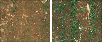
One of the 10 fields is selected for validation, and it is thus not included in the training of the model. By choosing an entire field for validation, we achieve a greater independence of the test and validation data, compared to a random selection of all the annotated images. The field that is selected for validation is the field in which the wheat is at the latest growth stage of the 10 fields. This field has a severe degree of occlusion compared to the others. By choosing the field in which there is greatest degree of occlusion, we risk reducing the system’s performance, but in return, we make clear one of the big challenges with automatic detection of weeds, which has to be solved in order to carry out precision weed control in cereal fields. The validation dataset consists of 153 images, containing 876 annotated weeds. Image samples from the training and validation-set can be seen in Figure 1.
Hand-annotated samples from (left) the training data and (right) the validation data. Notice the amount of occlusion in the image to the right.

Network architecture
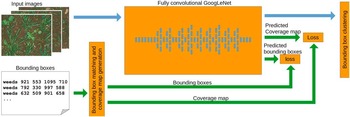
The convolutional neural network used for training is based on DetectNet by Nvidia (Barker, J. et al., Reference Barker, Sarathy and Tao2016). It consists of two parts: A fully convolutional neural network and a clustering function as illustrated in Figure 2. The fully convolutional neural network is trained by evaluating the errors in predicted bounding boxes and a predicted coverage map, which indicates detected locations of weeds in the image.
Network architecture. Input images and hand-made bounding boxed are fed into the network which produces a coverage map and bounding boxes. Green connections are only active during training. (after Barker, J. et al., (Reference Barker, Sarathy and Tao2016))

The fully convolutional neural network is based on the GoogLeNet architecture, from which the input layer and final pooling layer and inner product layer have been removed. Using an existing network allows one to use pre-trained models to initialize the network weights. Oquab et al. (Reference Oquab, Bottou, Laptev and Sivic2014) show that initializing convolutional neural networks with a model trained on a different data set causes the network to converge faster despite the fact that there are only few visual resemblances between the data set used for pretraining and the one used for training. GoogLeNet was designed for the ImageNet Challenge (Russakovsky et al. 2015). Therefore a model trained on the ImageNet data is used for initializing the weight in this study.
Network input and output
Images in which weeds are annotated with bounding boxes are required for training the network. These bounding boxes are used for generating a coverage map, which shows whether weeds are present at a given location in the image. This input coverage map for training is considered the “ground-truth” that we want the network output to match. The input coverage map is generated by rounding the corner coordinates of all bounding boxes to the nearest integer that is divisible by 16. Thereby each bounding box will fill a certain number of cells in a grid. Each cell in the grid are then assigned to a coverage value of 0 or 1, depending on whether a bounding box covers the grid cell. If the cell is covered, it is given a value of 1, otherwise 0. When testing the network, an image is the only required input.
As output, the fully convolutional neural network produces a new coverage map, in which each pixel corresponds to an area in the input image like for the input coverage map. This output coverage map shows how much the network believes that a plant is present at this location in the image. Along with the coverage map, the network outputs four bounding-box images. Each of these four bounding-box images contains pixel-values corresponding to the corner-coordinates of the bounding boxes.
Bounding box clustering
As described above, the network generates an output of five images; One coverage map and four bounding-box images. Here we will describe how these images are translated into bounding-boxes that mark the location of plants in the images.
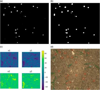
Figure 3 shows an example of a generated coverage map as well as the four bounding-box images. The first step is to make a binary threshold of the coverage map. The specific threshold value is not of great importance, as it is being set before training the network, which means that the network will be able to adapt its internal biases for the given threshold value. However, after training the network, the threshold can be lowered, which will cause the network to accept uncertain detections, or increased, which will cause the network to keep only the most certain detections.
Procedure of the bounding box generation. (a) coverage map produced by network. (b) threshold of (a). (c) offsets of x1,y1,x2 and y2 relative to white pixels in (b). (d) final annotated image.

For each white pixel in the thresholded coverage map, a bounding box is created. Each bounding box is specified by two coordinates, (x1,y1) and (x2,y2), defining the two opposite corners of the bounding box. The values of these two coordinates are extracted from the four bounding box-images, shown in Figure 3(c). The pixel values at a given location in each of these four images are the offsets of respectively x1, y1, x2 and y4, relative to the location of a white pixel in the coverage map.
As each cluster in the coverage map consists of several pixels, a lot of bounding boxes are generated, for each cluster. Therefore, in order to only get one bounding box for each plant, the bounding boxes are grouped together if the relative difference between the sides of the rectangles is less than a given threshold. Setting this threshold too high results in multiple detections of single plants, whereas setting it too low causes overlapping plants to be detected as one.
Network losses
The fully convolutional neural network and the bounding box predictor are trained simultaneously, where only the output of the bounding box predictor is used as cost for training both the network and the clustering function.
The sum of two cost functions is used for optimizing the network weights during the training phase. These losses are a coverage loss and a bounding box loss. The coverage loss is the mean square error of the coverage map predicted by the fully convolutional neural network and the coverage map generated from the annotated data. Because of this loss, all weeds in the training images must be annotated, as a missing plant in the training data will cause the coverage loss to increase.
 $$COV\_loss{\equals}{1 \over {2N}}\mathop{\sum}\limits_i^{i{\equals}N} {\left| {CM_{{inp}} (i){\minus}CM_{{pre}} (i)} \right|^{2} } $$
The other loss is the bounding box loss, which is the mean absolute difference of corners of the predicted bounding boxes and the input bounding boxes.
 $$BBOX\_loss{\equals}{1 \over {2N}}\mathop{\sum}\limits_i^{i{\equals}N} \matrix{ \Big(\left| {x_{{inp}}^{{min}} {\minus}x_{{pre}}^{{min}} } \right|{\plus}\left| {x_{{inp}}^{{max}} {\minus}x_{{pre}}^{{max}} } \right| \hfill \cr {\plus}\left| {y_{{inp}}^{{min}} {\minus}y_{{pre}}^{{min}} } \right|{\plus}\left| {y_{{inp}}^{{max}} {\minus}y_{{pre}}^{{max}} } \right|\Big) \hfill $$
These losses are calculated for each of the training images, but in order to stabilize the weight update, the losses are averaged over eight training images.
Evaluation
In order to evaluate the system’s ability to detect weeds, we need to set some matrix that indicates whether a weed is detected or not. To do so, we evaluate the Intersection Over Union (IOU), which evaluate the area a detected bounding box and an annotated bounding box have in common in proportion to the area that the annotation and detection cover together.
A plant is considered detected if the IOU is greater than ⅓, corresponding to a 50% overlap for two equal sized bounding-boxes, and if the center of the detection bounding box falls within the bounding box of the annotation and vice-versa. However, it is not enough to only consider the average IOU, since the IOU can be high while only few plants are detected. Therefore, we also measure the precision and recall.
The precision indicates the proportion of true positives relative to all detections. A high precision means that a large proportion of objects, identified as weeds by the algorithm, are also annotated as plants in the ground truth annotations. The recall, on the other hand, indicates the proportion of annotated plants that the algorithm has found automatically.
Results
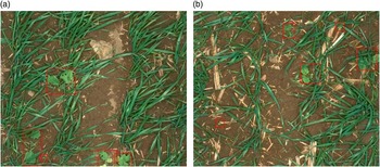
A total of 876 plants were annotated in the 153 validation images. During the evaluation, 406 of these 876 annotated plants were detected automatically by the algorithm. This yielded a recall of 46.3% and a precision of 86.6%. The average IOU for accepted detection is 0.64. The mean size of all the hand-annotated bounding boxes is 12.064 pixels, ranging from 702 pixels for the smallest annotation up to 247.123 pixels for the largest annotation. However, the mean size of the automatically detected bounding boxes is 15.006 pixels, which indicates that the algorithm encounters more difficulties in detecting smaller plants than it does in detecting the larger ones. The mean size of the bounding boxes of the plants that were not detected, is, therefore, a bit lower, with an average size of 9.534 pixels. Samples of the test image where the algorithm fail to detect the plants and detect all the plants is shown in Figure 4.
Samples from the validation dataset, where the algorithm (a) fails to detect the weeds and (b) detects all the weeds. The annotations in (a) is hand-made annotations in order to show the location of the missing plants. The annotations in (b) are made by the algorithm.

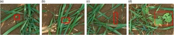
Plants that have not been detected, according to the IOU criteria, can generally be divided into four groups: small plants, plants exposed to heavy occlusion, grasses, and plants where only part of the plant has been detected. Figure 5 shows crops of the validation images, which exemplifies each of these cases: (a) small plant, (b) plant exposed to heavy occlusion, (c) grasses, (d), plants, where only part of it has been detected. Testing the method was carried out using an Nvidia TitanX (Pascal) GPU, which was able to process 20 images per second.
Plants that the algorithm fails to detect. (a) small plant, (b) plant exposed to heavy occlusion, (c) grasses, (d), plants, where only part of it has been detected. Markings in (a),(b) and (c) are hand-annotations, marking in (d) is made by the algorithm.

Discussion
Weed instances in cereal fields have been hard to detect automatically, as cereals are sown with a low distance, causing crops to overlap with weeds. Furthermore, the narrow row distance makes it hard to use spatial information for detecting the weeds as is possible for crops sown with larger row spacing, such as maize. Cereal is, however, the main crop in northern Europe, so to be able to perform precision weed control in cereal fields is essential. Therefore, one of the greatest accomplishments in this study is the ability to detect weed instances in winter wheat fields. The field, which was selected for validation, was a field with a severe degree of occlusion, which is partly the reason why not all weeds were detected.
It is believed, that the performance can be increased, by training the network with more images that contain overlapping plants. When training the network, it is important, that all weeds are annotated in the training data, as a detection of a plant, that is not annotated, will count as an error, causing the network to learn invalid pattern in the data. In the training data, which was used in this study, most weeds are annotated, but not all. A further increase of the recall is therefore expected, if the training data was fully annotated.
Detecting weeds is, however, not enough to determine optimal herbicide dosages, if the weed control is to be carried out chemically. In that case the network will be the first step of a two-step operation for determining plant species and weed infestation of fields, where the other step is an algorithm optimized for classification of the species, such as the method described in Dyrmann et al., (Reference Dyrmann, Karstoft and Midtiby2016). When selecting herbicides, it is important that grasses are not missed by the algorithm, as grasses are a strong competitor to the crops. However, detecting grasses is a challenge, due to the many visual similarities grass has with wheat. Further development is therefore necessary to make the algorithm better at detecting grasses.
Conclusion
In this paper a method capable of detecting weed instances in highly occluded cereal fields has been presented. Current methods for weed detection have, so far, had trouble with detecting weed instances in cereal fields due to heavy leaf occlusion. We addressed this problem of detecting weed instances in cereal fields by using a fully convolutional neural network that is based on a modified version of the GoogLeNet architecture. The network has been trained on thousands of annotated images, which has enabled the network to detect single weed instances in cereal fields despite heavy leaf occlusion. Results show that the algorithm is able to detect 46% of the weeds in a field, despite the fact that large parts of the weeds overlap with wheat plants. The algorithm, however, encounters problems in detecting very small weeds, grasses, and weeds exposed to a severe degree of overlap. In addition, the algorithm for large plants has trouble generating optimal bounding boxes that cover the whole plant.
Acknowledgements
This work was founded by GUDP (Grønt Udviklings- og DemonstrationsProgram) under the Ministry of Environment and Food of Denmark.