1 Introduction
The admissibility of expansion shock waves requires the so-called fundamental derivative of gas dynamics, introduced by Hayes (Reference Hayes1958) and Thompson (Reference Thompson1971) as
 $$\begin{eqnarray}\displaystyle {\it\Gamma}\equiv 1+\frac{{\it\rho}}{c}\left(\frac{\partial c}{\partial {\it\rho}}\right)_{s}, & & \displaystyle\end{eqnarray}$$
to be negative or to locally change its sign. In (1.1),
 ${\it\rho}$
is the density,
 $s$
is the entropy and
 $c$
is the thermodynamic sound speed, which is defined as
 $c\equiv \sqrt{(\partial P/\partial {\it\rho})_{s}}$
, where
 $P$
is the pressure. Note that for ideal gases
 ${\it\Gamma}$
is always positive under the assumption of constant specific heat capacities such as, for example, air at standard temperature and pressure, and consequently expansion shock waves are not physically admissible in constant-specific-heat dilute gases, a well-known result from gas dynamics textbooks, see e.g. Thompson (Reference Thompson1988).
Previous studies on non-classical gas dynamics, namely, the dynamics of fluids with
 ${\it\Gamma}<0$
, focused on so-called Bethe–Zel’dovich–Thompson (BZT) fluids (see e.g. Thompson Reference Thompson1971; Lambrakis & Thompson Reference Lambrakis and Thompson1972; Thompson & Lambrakis Reference Thompson and Lambrakis1973; Cramer & Kluwick Reference Cramer and Kluwick1984; Cramer & Sen Reference Cramer and Sen1986, Reference Cramer and Sen1987; Cramer Reference Cramer1989; Cramer, Tarkenton & Tarkenton Reference Cramer, Tarkenton and Tarkenton1992; Colonna & Guardone Reference Colonna and Guardone2006; Colonna, Guardone & Nannan Reference Colonna, Guardone and Nannan2007). BZT fluids are characterized by a highly complex molecular structure and molar mass and are predicted to exhibit negative-
 ${\it\Gamma}$
values in the single-phase vapour region to the right of the vapour–liquid critical point in the pressure–specific volume (
 $P$
–
 $v$
) thermodynamic plane. According to Guardone, Vigevano & Argrow (Reference Guardone, Vigevano and Argrow2004), the negative-
 ${\it\Gamma}$
region of a BZT fluid is approximately bounded by
 $0.75<P/P_{C}<1.0$
,
 $1.4<v/v_{C}<2.5$
and
 $0.96<T/T_{C}<1.01$
, where
 $T$
is the temperature and the subscript
 $C$
indicates critical-point values. Note that, since the critical region is approximately bounded by
 $0.96<T/T_{C}<1.04$
and
 $2/3<v/v_{C}<2$
, see Anisimov et al. (Reference Anisimov, Kiselev, Sengers and Tang1992), said region of negative nonlinearity occurs partly in this domain. Numerous authors (Thompson Reference Thompson1971; Thompson & Lambrakis Reference Thompson and Lambrakis1973; Cramer & Kluwick Reference Cramer and Kluwick1984; Cramer & Sen Reference Cramer and Sen1986; Cramer et al.
Reference Cramer, Kluwick, Watson and Pelz1986; Cramer Reference Cramer1987, Reference Cramer1989, Reference Cramer and Kluwick1991; Menikoff & Plohr Reference Menikoff and Plohr1989; Cramer & Fry Reference Cramer and Fry1993; Kluwick Reference Kluwick1993, Reference Kluwick2001; Argrow Reference Argrow1996; Brown & Argrow Reference Brown and Argrow1997, Reference Brown and Argrow2000; Fergason & Argrow Reference Fergason and Argrow2001; Fergason et al.
Reference Fergason, Ho, Argrow and Emanuel2001; Fergason, Guardone & Argrow Reference Fergason, Guardone and Argrow2003; Colonna, Guardone & Nannan Reference Colonna, Guardone and Nannan2006; Colonna et al.
Reference Colonna, Guardone and Nannan2007, Reference Colonna, Harinck, Rebay and Guardone2008, Reference Colonna, Nannan, Guardone and van der Stelt2009; Zamfirescu, Guardone & Colonna Reference Zamfirescu, Guardone and Colonna2008), identified diverse non-classical phenomena in BZT fluids, including rarefaction shock waves (RSW), composite wave fields such as mixed compressive shock fans or expansive fan-shock fans and double-sonic shock waves. Guardone, Zamfirescu & Colonna (Reference Guardone, Zamfirescu and Colonna2009) identified the so-called rarefaction shock region (RSR) of selected BZT fluids and its dependence on the molecular complexity of the fluid. The RSR is the domain bounded by the vapour–liquid equilibrium (VLE) curve and by the locus of the fluid states characterized by double-sonic rarefaction shock waves, namely, shock waves of finite intensity featuring sonic pre- and post-shock conditions in the shock reference. The RSR is located in the single-phase vapour region and it embeds the negative-
 ${\it\Gamma}$
domain.
The focus of this study is on non-classical gas dynamics effects other than those occurring in BZT fluids. In fact, the goal is to determine the admissibility region of rarefaction shock waves, namely, the RSR, in the vicinity of the vapour–liquid critical point, where scaled fundamental equations predict the existence of a negative-
 ${\it\Gamma}$
region for typical fluids.
It has been documented in a recent work of Nannan, Guardone & Colonna (Reference Nannan, Guardone and Colonna2013) that due to criticality, the fundamental derivative of gas dynamics becomes negative in the vapour–liquid equilibrium region of pure typical fluids. This result is valid under the assumption that the phases are homogeneously and finely dispersed, i.e. there is neither agglomeration, nor stratification as a consequence of a gravitational or some other potential force field. In addition, the influence of surface tension is assumed negligible; near criticality the surface tension has low values and goes to zero at the critical point itself. Note that here ‘typical fluid’ implies a substance wherein the molecular interactions are governed by short-range forces corresponding to a so-called three-dimensional Ising-like system (Sengers & Levelt-Sengers Reference Sengers and Levelt-Sengers1984): examples of such fluids are water, carbon dioxide, methane (alkanes) and sulphur hexafluoride. Vapours of metals and salts as well as plasmas are therefore excluded. In the following, methane, ethylene and carbon dioxide are chosen as exemplary typical fluids.
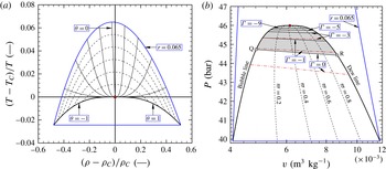
The fact that
 ${\it\Gamma}$
is negative in the two-phase critical region – see for example figure 1 for methane and the thermodynamic model discussed in § 2 – implies that expansion shock waves, specifically those exhibiting phase transition such as condensation shock waves, are physically admissible (Nannan, Guardone & Colonna Reference Nannan, Guardone and Colonna2014). Moreover, since positive values of
 ${\it\Gamma}$
are expected in the VLE region sufficiently far from the vapour–liquid critical point, rarefaction shock waves characterized by sonic post-shock Mach numbers as well as composite wave fields are physically admissible, similarly to what is observed for BZT fluids.
The vapour–liquid critical region of methane computed using the scaled fundamental EoS of Kurumov, Olchowy & Sengers (Reference Kurumov, Olchowy and Sengers1988). (a) Isolines of
 $r$
and
 ${\it\theta}$
in the density–temperature plane. The locus
 ${\it\theta}=-1$
is the dew line,
 ${\it\theta}=1$
is the bubble line. The region limited by the solid blue lines represents the validity domain of the scaled fundamental EoS for methane as reported by Kurumov et al. (Reference Kurumov, Olchowy and Sengers1988) under the hypothesis of thermodynamic equilibrium. (b) Pressure–volume thermodynamic plane. Points Q and R are located on the
 ${\it\Gamma}=0$
line traversing the VLE region in the limit of the vapour mass fraction
 ${\it\varpi}$
approaching 0 and 1, respectively;
 ${\it\Gamma}\rightarrow -\infty$
as the critical point is approached from the two-phase region. The shaded area denotes the domain of negative nonlinearity, i.e.
 ${\it\Gamma}<0$
. For comparison, some iso-
 ${\it\Gamma}$
lines have also been computed using the reference EoS of Setzmann & Wagner (Reference Setzmann and Wagner1991); these are the red dashed-dotted lines.

Two important remarks arguably put the following treatment in the correct perspective. Firstly, this study is different from the work of Thompson, Carofano & Kim (Reference Thompson, Carofano and Kim1986) in the sense that the wave fields and shock waves discussed therein are a consequence of
 ${\it\Gamma}$
being negative infinity (
 $-\infty$
) at the bubble line due to the discontinuity of the thermodynamic sound speed at the phase boundary. The cited reference reports how the thermodynamic sound speed in the VLE region is always less than, or at most equal to, the sound speed in the single-phase region at the saturation boundary, see equation (15) ibid. Secondly, it is worth noting that Borisov, Kutateladze & Nakoryakov (Reference Borisov, Kutateladze and Nakoryakov1983) and Kutateladze, Nakoryakov & Borisov (Reference Kutateladze, Nakoryakov and Borisov1987) document the experimental observation of a steady rarefaction shock wave, claiming that it occurs in the single-phase vapour region of fluid R-13 (CClF
 $_{3}$
). However, on the basis of arguments and computations presented by Fergason & Argrow (Reference Fergason and Argrow2001), Fergason et al. (Reference Fergason, Ho, Argrow and Emanuel2001), Fergason et al. (Reference Fergason, Guardone and Argrow2003) and recently by Nannan et al. (Reference Nannan, Guardone and Colonna2013), the results of Borisov et al. provide inconclusive evidence of the occurrence of such an event. The measured pressure signal can be explained in different ways, and one of the hypotheses is that the flow under scrutiny occurred partly within the two-phase thermodynamic region.
The structure of this document is as follows: § 2 presents an overview of the equation of state adopted to calculate the fluid properties, and summarizes results for the fundamental derivative of gas dynamics in the vapour–liquid equilibrium region. Sections 3–5 review the so-called shock admissibility conditions, which are employed to determine, int. al., the physical admissibility of rarefaction shock waves, and the fluid states which maximize the speed and pressure change across the wave. These thermodynamic states form the locus of post-shock states of pure rarefaction shock waves admitting, for a given pre-shock state, sonic post-shock states, and define the region of admissibility of rarefaction shock waves within the VLE region. Section 6 presents a discussion on the assumptions on which the computations are based, and provides concluding remarks.
2 The scaled fundamental equation of state
As it is well known, several thermodynamic and transport properties either diverge or go to zero at the vapour–liquid critical point; the slope of the
 $P$
–
 $T$
curve is however an exception, see, e.g. Levelt-Sengers (Reference Levelt-Sengers1970). Notable examples of anomalous trends include the weak divergence of the isochoric heat capacity
 $c_{v}$
, the strong divergence of the isothermal compressibility
 ${\it\kappa}_{T}\equiv -1/v(\partial v/\partial P)_{T}$
, the weak approach to zero of the thermodynamic (zero-frequency) sound speed at the critical point and the strong divergence of the thermal conductivity, see for example the works of Michels, Sengers & van der Gulik (Reference Michels, Sengers and van der Gulik1962), Levelt-Sengers, Kamgar-Parsi & Sengers (Reference Levelt-Sengers, Kamgar-Parsi and Sengers1983a
), Levelt-Sengers, Morrison & Chang (Reference Levelt-Sengers, Morrison and Chang1983b
), Albright et al. (Reference Albright, Edwards, Chen and Sengers1987), Kurumov et al. (Reference Kurumov, Olchowy and Sengers1988) and Wyczalkowska & Sengers (Reference Wyczalkowska and Sengers1999) and listed references therein reporting corresponding experimental data. The Helmholtz free energy is non-analytic at the critical point, as a direct consequence of the divergence of
 $c_{v}$
near the critical point. Consequently, classical equations of state (EoS) cannot correctly model the vapour–liquid critical region. The limitations of cubic equations of state in this respect are well known, but even the modern, most accurate multi-parameter equations of state, including those incorporating so-called critical terms in their functional form (Lemmon, Huber & McLinden Reference Lemmon, Huber and McLinden2007), cannot accurately predict the primary thermodynamic properties and even more so secondary or derived properties at the critical point. Colonna et al. (Reference Colonna, Nannan, Guardone and van der Stelt2009) and Nannan et al. (Reference Nannan, Guardone and Colonna2013) pointed out that even the highly accurate reference model of Wagner Setzmann containing critical terms cannot provide correct evaluations of
 ${\it\Gamma}$
if the considered fluid states are close enough to the critical point.
The critical-point thermodynamics of fluids whose molecular interactions are governed by short-range forces, also called three-dimensional Ising-like systems, is described via scaled fundamental EoS (Levelt-Sengers Reference Levelt-Sengers1970; Wegner Reference Wegner1972; Levelt-Sengers et al.
Reference Levelt-Sengers, Morrison and Chang1983b
; Sengers & Levelt-Sengers Reference Sengers and Levelt-Sengers1984). In particular, near the critical point the thermodynamic potential of a spin system represented by a Landau–Ginzburg–Wilson Hamiltonian can be described by an expansion as provided by the EoS in (2.2) below. The EoS (2.2) is formulated in terms of
 $P/T$
as a function of
 $1/T$
and
 ${\it\mu}/T$
, where
 $P/T$
is the potential and
 ${\it\mu}$
is the chemical potential. Note that
 $P({\it\mu},T)$
is a fundamental (canonical) thermodynamic equation, therefore all properties can be determined from it using combinations of its first-, second-, and/or higher-order derivatives, see Callen (Reference Callen1985). The EoS is made dimensionless by critical-point values, namely
 $$\begin{eqnarray}\displaystyle \tilde{P}\equiv \frac{P}{T}\frac{T_{C}}{P_{C}},\quad \tilde{T}\equiv -\frac{T_{C}}{T},\quad \tilde{{\it\mu}}\equiv \frac{{\it\mu}}{T}\frac{{\it\rho}_{C}T_{C}}{P_{C}}. & & \displaystyle\end{eqnarray}$$
The functional form of the scaled fundamental EoS reads
 $$\begin{eqnarray}\displaystyle \tilde{P}=1+\mathop{\sum }_{i=1}^{3}\tilde{P}_{i}({\rm\Delta}\tilde{T})^{i}+{\rm\Delta}\tilde{{\it\mu}}(1+\tilde{P}_{11}{\rm\Delta}\tilde{T})+{\rm\Delta}\tilde{P}. & & \displaystyle\end{eqnarray}$$
In (2.2),
 $\tilde{P}_{i=1,\ldots ,3}$
and
 $\tilde{P}_{11}$
are pressure background parameters and are fluid specific. Furthermore,
 $$\begin{eqnarray}\displaystyle {\rm\Delta}\tilde{T}=\tilde{T}+1,\quad {\rm\Delta}\tilde{{\it\mu}}=\tilde{{\it\mu}}-\tilde{{\it\mu}}_{C}-\mathop{\sum }_{i=1}^{4}\tilde{{\it\mu}}_{i}({\rm\Delta}\tilde{T})^{i}, & & \displaystyle\end{eqnarray}$$
where
 $\tilde{{\it\mu}}_{i=1,\ldots ,4}$
and
 $\tilde{{\it\mu}}_{C}$
are thermal background parameters peculiar to each fluid. The singular part of (2.2), i.e.
 ${\rm\Delta}\tilde{P}$
, is expressed as a function of the universal critical exponents
 ${\it\beta}$
,
 ${\it\delta}$
and
 ${\it\Delta}_{1}$
, of the substance-specific parameters
 $a$
,
 $k_{0}$
and
 $k_{1}$
, and of the auxiliary functions
 $p_{0}({\it\theta})$
,
 $p_{1}({\it\theta})$
and
 $r$
.
 ${\it\theta}$
and
 $r$
are parametric variables allowing the model to conform with the asymptotic and symmetry requirements of the Ising model.
The dependence of
 ${\rm\Delta}\tilde{P}$
on variables
 $r$
and
 ${\it\theta}$
was first approximated by Schofield, Litster & Ho (Reference Schofield, Litster and Ho1969) and later extended by Balfour et al. (Reference Balfour, Sengers, Moldover and Levelt-Sengers1978), who introduced the first correction-to-scaling term, resulting in the so-called revised and extended linear model, which has been used for the computations herein. Its functional expression reads
 $$\begin{eqnarray}\displaystyle {\rm\Delta}\tilde{P}=ar^{{\it\beta}({\it\delta}+1)}[k_{0}p_{0}({\it\theta})+r^{{\it\Delta}_{1}}k_{1}p_{1}({\it\theta})]. & & \displaystyle\end{eqnarray}$$
Variables
 $r$
and
 ${\it\theta}$
in (2.4) describe respectively the distance of a thermodynamic state with respect to the critical point and the location of a thermodynamic state on a line of constant
 $r$
, such that
 ${\it\theta}=+1$
represents the saturated liquid line and
 ${\it\theta}=-1$
represents the saturated vapour line (
 $-1\leqslant {\it\theta}\leqslant +1$
) and
 $r$
is bounded and at least zero. The functions
 ${\rm\Delta}\tilde{T}$
and
 ${\rm\Delta}\tilde{{\it\mu}}$
can be rewritten as, see Balfour et al. (Reference Balfour, Sengers, Moldover and Levelt-Sengers1978):
 $$\begin{eqnarray}\displaystyle {\rm\Delta}\tilde{T}=r(1-b^{2}{\it\theta}^{2})-\mathfrak{c}{\rm\Delta}\tilde{{\it\mu}},\quad {\rm\Delta}\tilde{{\it\mu}}=ar^{{\it\beta}{\it\delta}}{\it\theta}(1-{\it\theta}^{2}), & & \displaystyle\end{eqnarray}$$
where
 $b^{2}$
is a universal constant and
 $\mathfrak{c}$
is a fluid-specific parameter. All primary and derivative thermodynamic properties in the single- and two-phase region can be obtained from (2.2), see Nannan et al. (Reference Nannan, Guardone and Colonna2013) for relevant expressions.
Starting from (2.1) to (2.5), Nannan et al. (Reference Nannan, Guardone and Colonna2013) showed that: (i)
 ${\it\Gamma}$
weakly diverges to large positive values as the critical point is approached from the single-phase region, namely, the power of divergence of
 ${\it\Gamma}$
as a function of the dimensionless temperature difference with respect to the critical temperature is less than unity, and (ii)
 ${\it\Gamma}$
weakly diverges to large negative values as the critical point is approached along the critical isochore from the vapour–liquid equilibrium region, thus implying the existence of a domain of so-called negative nonlinearity in any typical fluid, where
 ${\it\Gamma}<0$
. Figure 1(b) shows the thermodynamic region encompassing states featuring negative
 ${\it\Gamma}$
for methane (CH
 $_{4}$
), calculated using the substance-specific parameters reported by Kurumov et al. (Reference Kurumov, Olchowy and Sengers1988). In particular, along the dew line, one has
 $$\begin{eqnarray}\displaystyle \lim _{T\uparrow T_{C}}{\it\Gamma}(P^{sat}(T),T)\propto \lim _{T\uparrow T_{C}}\left[\frac{T-T_{C}}{T}\right]^{-\tilde{{\it\alpha}}}=\lim _{T\uparrow T_{C}}-\frac{T-T_{C}}{T}\left|\frac{T-T_{C}}{T}\right|^{-(\tilde{{\it\alpha}}+1)}\rightarrow +\infty , & & \displaystyle\end{eqnarray}$$
where
 $P^{sat}(T)$
is the saturation pressure at temperature
 $T$
and
 $\tilde{{\it\alpha}}$
is the critical exponent,
 $\tilde{{\it\alpha}}=0.890\pm 0.003$
, see Nannan et al. (Reference Nannan, Guardone and Colonna2013) (
 $\tilde{{\it\alpha}}$
should not be confused with
 ${\it\alpha}$
, which is a universal constant used in common literature on critical point effects; herein,
 $\tilde{{\it\alpha}}=1-{\it\alpha}$
). Note that
 $\tilde{{\it\alpha}}$
is a universal constant for all fluids belonging to the class of three-dimensional Ising-like systems. Similarly, along the critical isochore in the single-phase region,
 $$\begin{eqnarray}\displaystyle \lim _{T\downarrow T_{C}}{\it\Gamma}({\it\rho}_{C},T)\propto \lim _{T\downarrow T_{C}}\frac{T-T_{C}}{T}\left|\frac{T-T_{C}}{T}\right|^{-(\tilde{{\it\alpha}}+1)}\rightarrow +\infty . & & \displaystyle\end{eqnarray}$$
The divergence of
 ${\it\Gamma}$
to positive values in the single-phase critical region is in agreement with the observation of Emanuel (Reference Emanuel1996) (see also Gulen, Thompson & Cho Reference Gulen, Thompson, Cho, Meier and Thompson1989; Kluwick Reference Kluwick, Morioka and van Wijngaarden1995). If the critical point is approached along the critical isochore from within the vapour–liquid equilibrium region,
 ${\it\Gamma}$
weakly diverges to large, negative values according to
 $$\begin{eqnarray}\displaystyle \lim _{T\uparrow T_{C}}{\it\Gamma}({\it\rho}_{C},T)\propto \lim _{T\uparrow T_{C}}\frac{T-T_{C}}{T}\left|\frac{T-T_{C}}{T}\right|^{-(\tilde{{\it\alpha}}+1)}\rightarrow -\infty . & & \displaystyle\end{eqnarray}$$
It is remarkable that the above power-law relations (2.6)–(2.8) are valid for any pure typical fluid belonging to the three-dimensional Ising universality class.
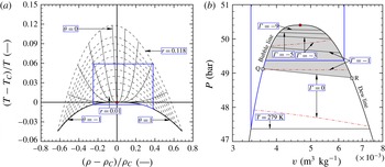
The vapour–liquid critical region of ethylene computed using the scaled fundamental EoS of Sengers, Greer & Sengers (Reference Sengers, Greer and Sengers1976). (a) Representation in the density–temperature plane in terms of the parametric variables
 $r$
–
 ${\it\theta}$
. The region delimited by the solid blue lines shows the validity domain of the scaled fundamental EoS of Sengers et al. (Reference Sengers, Greer and Sengers1976) under the hypothesis of thermodynamic equilibrium. (b) Pressure–volume thermodynamic plane. The shaded area denotes the domain of negative nonlinearity, i.e.
 ${\it\Gamma}<0$
. For comparison, some iso-
 ${\it\Gamma}$
lines have also been computed using the reference EoS of Smukala, Span & Wagner (Reference Smukala, Span and Wagner2000); these are the red dashed-dotted lines.

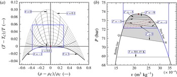
The vapour–liquid critical region of carbon dioxide computed using the scaled fundamental equation of state of Albright et al. (Reference Albright, Edwards, Chen and Sengers1987). (a) Representation in the density–temperature plane in terms of the parametric variables
 $r$
–
 ${\it\theta}$
. The region circumscribed by the solid blue lines corresponds to the validity domain of the EoS as provided by Albright et al. (Reference Albright, Edwards, Chen and Sengers1987) under the hypothesis of thermodynamic equilibrium. (b) Pressure–volume thermodynamic plane. The shaded area denotes the domain of negative nonlinearity, i.e.
 ${\it\Gamma}<0$
. For comparison, some iso-
 ${\it\Gamma}$
lines have also been computed using the reference EoS of Span & Wagner (Reference Span and Wagner1996); these are the red dashed-dotted lines.

Isolines of the fundamental derivative of gas dynamics
 ${\it\Gamma}$
are reported in figure 1(b) for methane, which exhibits a region of negative nonlinearity bounded by the dew and bubble line and by the
 ${\it\Gamma}=0$
isoline QR, where states Q and R are respectively located in the limit of the vapour fraction going to zero and one (note that the region of negative nonlinearity has a vapour mass fraction between zero and one,
 $0<{\it\varpi}<1$
). The VLE region and the negative-
 ${\it\Gamma}$
region are shown in figures 2 and 3 for ethylene (C
 $_{2}$
H
 $_{4}$
; EoS of Sengers et al. (Reference Sengers, Greer and Sengers1976)) and carbon dioxide (CO
 $_{2}$
; EoS of Albright et al. (Reference Albright, Edwards, Chen and Sengers1987)), respectively.
Since the negative-
 ${\it\Gamma}$
region extends outside the region of validity of the scaling EoS for C
 $_{2}$
H
 $_{4}$
and CO
 $_{2}$
, reference EoS are used to confirm that predictions from scaling laws are qualitatively, though not quantitatively, valid also away from the critical point, see figures 1(b), 2(b) and 3(b). Note that reference EoS are not valid in the close proximity of the critical point and therefore one cannot expect that the iso-
 ${\it\Gamma}$
lines (including the curvature) computed using reference EoS are coincident with those obtained by the scaling laws in the critical point region. A thorough comparison of the values of the fundamental derivative of gas dynamics
 ${\it\Gamma}$
computed by reference and scaling EoS is reported in Nannan et al. (Reference Nannan, Guardone and Colonna2013).
The existence of fluid thermodynamic states characterized by negative values of
 ${\it\Gamma}$
in the near-critical vapour–liquid equilibrium region results in the admissibility of expansive shock waves in and around this thermodynamic domain. The derivation of the conditions for shock wave admissibility is presented in the following section.
3 Admissibility conditions for shock waves
Once a shock wave is formed, a description of the wave field not accounting for the shock wave structure requires the use of the Rankine–Hugoniot jump conditions. The deduction of these relations between pre- and post-shock states, A and B respectively, is based upon the laws of conservation of mass, momentum and energy applied to a control volume which locally encloses the shock front and which moves with the shock wave velocity. Under the additional hypothesis that the shock wave represents a discontinuity separating two regions of thermodynamic equilibrium states, as seen by an observer moving with the shock wave, and after some symbolic manipulation, the following system of equations is obtained
 $$\begin{eqnarray}\displaystyle & \displaystyle J={\it\rho}_{A}\boldsymbol{u}_{A}\boldsymbol{\cdot }\boldsymbol{n}={\it\rho}_{B}\boldsymbol{u}_{B}\boldsymbol{\cdot }\boldsymbol{n}, & \displaystyle\end{eqnarray}$$
 $$\begin{eqnarray}\displaystyle & \displaystyle P_{B}-P_{A}+J^{2}(v_{B}-v_{A})=0, & \displaystyle\end{eqnarray}$$
 $$\begin{eqnarray}\displaystyle & \displaystyle h_{B}-h_{A}+{\textstyle \frac{1}{2}}(v_{A}+v_{B})(P_{B}-P_{A})=0, & \displaystyle\end{eqnarray}$$
 $J$
is the mass flux across the shock wave,
 $\boldsymbol{u}$
is the velocity vector,
 $\boldsymbol{n}$
is the normal vector to the shock wave surface and
 $h=h(P,v)$
is the enthalpy. Relation (3.3), which involves thermodynamic quantities only, is usually referred to as the shock adiabat or Rankine–Hugoniot curve and it provides the implicit definition of the post-shock pressure
 $P_{B}$
as a function of the post-shock specific volume
 $v_{B}$
for a given pre-shock state
 $(P_{A},v_{A})$
, namely,
 $P_{B}=P^{HR}(v_{B};P_{A},v_{A})$
. Relation (3.2) is the so-called Rayleigh line. In the pressure–specific volume (
 $P$
–
 $v$
) diagram, the Rayleigh line is a straight line with slope
 $-J^{2}$
connecting points
 $(P_{A},v_{A})$
and
 $(P_{B},v_{B})$
. The intersection of the Rayleigh line and the shock adiabat in the
 $P$
–
 $v$
diagram implies simultaneous conservation of mass, momentum and energy across the shock wave connecting points A and B, namely,
 $$\begin{eqnarray}\displaystyle P^{RH}(v_{B};P_{A},v_{A})=P_{A}-J^{2}(v_{B}-v_{A}) & & \displaystyle\end{eqnarray}$$
for a given value of
 $J$
.
Yet, relations (3.1)–(3.3) are insufficient to discern physically admissible from inadmissible solutions, as it is typical of the application of the first law of thermodynamics only. Since a shock wave exhibits non-negligible gradients in temperature and velocity, the entropy of the flow passing through the shock wave must increase, because of irreversible processes occurring within the shock wave. In addition to the entropy-increase criterion prescribed by the second law of thermodynamics, the Lax–Oleinik condition for mechanical stability (Lax Reference Lax1957; Oleinik Reference Oleinik1959) must also be fulfilled. Mathematically, the set of equations (3.1)–(3.3) is extended to include
 $$\begin{eqnarray}\displaystyle & \displaystyle [s]\geqslant 0, & \displaystyle\end{eqnarray}$$
 $$\begin{eqnarray}\displaystyle & \displaystyle Ma_{A\boldsymbol{n}}\geqslant 1\geqslant Ma_{B\boldsymbol{n}}. & \displaystyle\end{eqnarray}$$
 $Ma_{A\boldsymbol{n}}\equiv (u_{\boldsymbol{n}}/c)_{A}$
and
 $Ma_{B\boldsymbol{n}}\equiv (u_{\boldsymbol{n}}/c)_{B}$
.
The analysis of shock wave admissibility is facilitated by the use of graphical information obtained from the
 $P$
–
 $v$
diagram of the fluid, where the shock adiabat and the straight Rayleigh line can be drawn once the pre-shock state, A, is prescribed. Conditions (3.5)–(3.6) can then be employed to obtain admissible post-shock states, B. As demonstrated by Kluwick (Reference Kluwick2001) and Zamfirescu et al. (Reference Zamfirescu, Guardone and Colonna2008), if the Rayleigh line from a state A to a state B is located completely above the shock adiabat pinned on A and passing through B, then only admissible self-similar solutions are either compression shock waves or isentropic expansion fans, according to relations (3.1)–(3.3) and conditions (3.5)–(3.6).
Jump A–B is therefore an admissible compression shock wave in the
 $P$
–
 $v$
diagram. On the contrary, if the Rayleigh line from a state A to a state B is located completely below the shock adiabat pinned on A and passing through B, then only rarefaction shock waves or compression fans are possible. Also in this case all relations/conditions (3.1)–(3.3) and (3.5)–(3.6) are satisfied, and jump A–B is then an admissible rarefaction shock wave. Therefore, for an admissible shock wave one has
 $$\begin{eqnarray}\displaystyle \left[\frac{\text{d}}{\text{d}v}P^{RH}(v;P_{A},v_{A})\right]_{B}\leqslant \frac{P_{B}-P_{A}}{v_{B}-v_{A}}\leqslant \left[\frac{\text{d}}{\text{d}v}P^{RH}(v;P_{A},v_{A})\right]_{A}. & & \displaystyle\end{eqnarray}$$
In particular, sonic pre- and post-shock cases are identified by the following conditions
 $$\begin{eqnarray}\displaystyle \frac{P_{B}-P_{A}}{v_{B}-v_{A}}=\left\{\begin{array}{@{}c@{}}\displaystyle \left[\frac{\text{d}}{\text{d}v}P^{RH}(v;P_{A},v_{A})\right]_{A}\quad \text{Pre-shock sonic at point A},\\ \displaystyle \left[\frac{\text{d}}{\text{d}v}P^{RH}(v;P_{A},v_{A})\right]_{B}\quad \text{Post-shock sonic at point B}.\end{array}\right. & & \displaystyle\end{eqnarray}$$
Moreover, for the solution of the Riemann problem to be unique, the Grüneisen coefficient must be positive in the post-shock state, see Kluwick (Reference Kluwick2001). This is indeed always the case in both the single- and the two-phase critical point region, since one has
 $$\begin{eqnarray}\displaystyle G=\left(\frac{\partial P}{\partial e}\right)_{v}=\frac{1}{c_{v}}\frac{\text{d}P^{sat}}{\text{d}T}\geqslant 0, & & \displaystyle\end{eqnarray}$$
where
 $e$
is the specific internal energy,
 $(\text{d}P^{sat}/\text{d}T)$
is the slope of the vapour pressure curve in the
 $P$
–
 $T$
thermodynamic plane and
 $c_{v}$
is the specific heat capacity at constant volume. The derivative
 $\text{d}P^{sat}/\text{d}T$
is positive for a pure fluid also in the vicinity of the critical point (it is one of the few properties that does not diverge or go to zero) and
 $c_{v}$
diverges to large, yet always positive, values. Therefore
 $G$
approaches zero from the positive side.
4 Expansion waves through the domain of negative-
 ${\it\Gamma}$
values

Expansion waves featuring negative
 ${\it\Gamma}$
are described here. For illustrative purposes, a single isentropic line
 $s=\bar{s}$
crossing the negative-
 ${\it\Gamma}$
VLE region is considered. Along this isentrope, a number of exemplary candidate pre-shock states
 $A$
are selected and the admissibility of either rarefaction shock waves or composite waves, including a sonic shock, is studied with the help of the geometrical arguments valid in a
 $P$
–
 $v$
diagram as outlined in § 3,
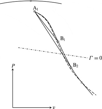
Representative shock waves in the
 $P$
–
 $v$
plane from a pre-shock state A
 $_{1}$
in the negative-
 ${\it\Gamma}$
VLE region. The continuous curve through A
 $_{1}$
, B
 $_{1}$
and B
 $_{2}$
is the shock adiabat centred in A
 $_{1}$
, the continuous curve on the top is the VLE boundary (the symbol indicate the critical point), straight lines connecting A
 $_{1}$
to B
 $_{1}$
and B
 $_{2}$
are Rayleigh lines, the dashed line indicates an isentrope passing through point A
 $_{1}$
(
 $s_{A_{1}}$
); it eventually intersects the Rankine–Hugoniot line pinned on A
 $_{1}$
at the state indicated by the triangle symbol. The line indicated by dash-dots is the
 ${\it\Gamma}=0$
line in the VLE region.

We start by commenting on figure 4, where the candidate pre-shock state A
 $_{1}$
,
 $s_{A_{1}}=\bar{s}$
, is located in the negative-
 ${\it\Gamma}$
VLE region. Candidate post-shock states B, located along the shock adiabat through A
 $_{1}$
, lie either in the negative-
 ${\it\Gamma}$
VLE region (such as for example state B
 $_{1}$
in figure 4) or in the positive-
 ${\it\Gamma}$
VLE region (state B
 $_{2}$
). Shock waves such as jump A
 $_{1}$
–B
 $_{1}$
satisfy the shock admissibility conditions (3.1)–(3.3) and (3.5)–(3.6), because the Rayleigh line connecting these two states is located completely below the Rankine–Hugoniot line centred on A
 $_{1}$
and passing through B
 $_{1}$
. Moreover, rarefaction shock wave A
 $_{1}$
–B
 $_{1}$
exhibits a supersonic-to-subsonic speed transition. Another admissible shock wave, arguably more interesting than the first example, is that denoted associated jump A
 $_{1}$
–B
 $_{2}$
. Also in this case the shock wave is admissible because the Rayleigh line connecting A
 $_{1}$
to B
 $_{2}$
is located completely below the shock adiabat pinned on A
 $_{1}$
and passing through B
 $_{2}$
. However, for this particular shock wave, the Rayleigh line is tangent to the involved shock adiabat at the post-shock state, B
 $_{2}$
, and consequently, this shock wave displays a supersonic-to-sonic speed transition. All rarefaction waves connecting state A
 $_{1}$
to any post-shock state located between A
 $_{1}$
and B
 $_{2}$
along the shock adiabat through A
 $_{1}$
are admissible. No rarefaction shock is admissible for post-shock states past B
 $_{2}$
.
Illustration of the same type of rarefaction shock waves of figure 4. Here however, state A
 $_{2}$
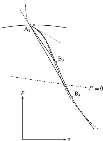
is located near the bubble or the dew line such that the vapour mass fraction approaches zero. Legend: as in figure 4. Furthermore, the dotted lines above and below the bubble line illustrate the discontinuity in slope of the isentrope due to phase change.

Next, in figure 5, the pre-shock state A
 $_{2}$
,
 $s_{A_{1}}=s_{A_{2}}=\bar{s}$
, is located in the VLE region very close to either the bubble or the dew line. For states close to saturation, the vapour mass fraction
 ${\it\varpi}\downarrow 0$
or
 ${\it\varpi}\uparrow 1$
, with
 ${\it\varpi}=0$
and
 ${\it\varpi}=1$
constituting single-phase thermodynamic states. Using the geometrical arguments in § 3, rarefaction shock waves A
 $_{2}$
–B
 $_{3}$
and A
 $_{2}$
–B
 $_{4}$
are admissible solutions of the shock admissibility conditions (3.1)–(3.3) and (3.5)–(3.6), with the peculiar jump A
 $_{2}$
–B
 $_{4}$
which displays a supersonic-to-sonic speed transition. An additional finding is that the shock wave A
 $_{2}$
–B
 $_{4}$
displays the greatest pre-shock supersonic speed for all possible pre-shock state located along the isentrope
 $s=\bar{s}$
, see § 5 below.
State A
 $_{3}$
is located in the single-phase critical region and
 $s_{A_{1}}=s_{A_{2}}=s_{A_{3}}$
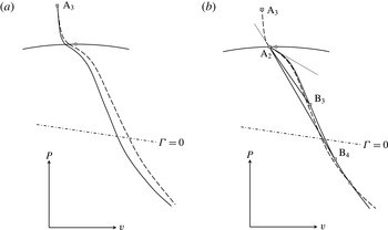
(see figures 4 and 5). Legend as in figure 4. Furthermore, the dotted lines above and below the dew line illustrate the discontinuity in slope of the isentrope due to phase change. (a) Rarefaction shock waves from state A
 $_{3}$
are, in principle, impossible because any Rayleigh line drawn is not completely below the shock adiabat centred on A
 $_{3}$
. Very close to the critical point a special situation occurs; this is discussed in § 5. (b) A possible composite expansive wave would ensue given a high-pressure state corresponding to A
 $_{3}$
and a low-pressure state corresponding to, say, B
 $_{4}$
, namely an isentropic expansion fan connecting states A
 $_{3}$
and A
 $_{2}$
immediately followed by jump A
 $_{2}$
–B
 $_{4}$
.

With reference to figure 6, consider as a third case a pre-shock state A
 $_{3}$
located on the same isentrope of figures 4 and 5, i.e.
 $s_{A_{1}}=s_{A_{2}}=s_{A_{3}}=\bar{s}$
. In principle, a pure rarefaction shock wave from state A
 $_{3}$
is impossible because a Rayleigh line drawn from A
 $_{3}$
can never be located completely below the shock adiabat centred on A
 $_{3}$
, see figure 6(a). There is however an exception on said constraint, which is valid for single-phase fluid states very close to the critical point; this particular case is discussed near the end of the next section. On the contrary, from state A
 $_{3}$
, a composite wave fields is possible up to states B
 $_{3}$
or B
 $_{4}$
, see figure 6(b). The first part of the composite wave field displays an isentropic expansion fan connecting states A
 $_{3}$
and A
 $_{2}$
, subsequently followed by a pressure discontinuity starting from A
 $_{2}$
(a shock adiabat therefore has to be drawn, pinned on A
 $_{2}$
). Two of such permissible rarefaction shock waves after the expansion fan are A
 $_{2}$
–B
 $_{3}$
and A
 $_{2}$
–B
 $_{4}$
, depending on the prescribed low-pressure value, as discussed above for figure 5. Note that in figure 6 the Rankine–Hugoniot line centred on A
 $_{3}$
and depicted in figure 6(a) is different from that pinned on A
 $_{2}$
(shown in figure figure 6
b), however it is selected such that
 $s_{A_{2}}=s_{A_{3}}$
.
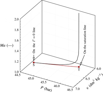
Exemplary (pre-shock) Mach locus (solid black line) for methane, computed by selecting several thermodynamic points within the region of negative nonlinearity, on an a selected isentrope
 $s_{i}$
(red curve), chosen as pre-shock states, and subsequently using system (3.1)–(3.3) and (3.5)–(3.6) to determine admissible rarefaction shock waves along this isentrope associated with sonic post-shock speeds.

The shock Mach number of rarefaction shock waves originating from a given point A along the isentrope
 $s=\bar{s}$
crossing the negative-
 ${\it\Gamma}$
region is now discussed. For a given rarefaction shock wave, the shock Mach number is defined as
 $Ma_{S}=u_{S}/c_{A}$
, with
 $u_{S}$
denoting pre-shock fluid velocity in the shock reference. In a still fluid,
 $u_{S}$
is the shock velocity in the laboratory reference frame. Note that the value of
 $Ma_{S}$
depends on the pre-shock thermodynamic state, for example on the pre-shock entropy
 $s_{A}$
and specific volume
 $v_{A}$
, and the e.g. specific volume
 $v_{B}$
at the post-shock state B. Therefore,
 $Ma_{S}=Ma_{S}(v_{B};s_{A},v_{A})$
. For each pre-shock point A along a given isentrope
 $s=\bar{s}$
, the maximum shock Mach number is therefore computed as
 $$\begin{eqnarray}\displaystyle \widehat{Ma}_{S}(\bar{s},v_{A})=\max _{v_{B}\in \mathscr{V}(\bar{s},v_{A})}Ma_{S}(v_{B};\bar{s},v_{A}), & & \displaystyle\end{eqnarray}$$
where
 $\mathscr{V}(s_{A},v_{A})$
is the set of admissible specific volumes of post-shock states corresponding to the pre-shock state A. In particular, along a given isentrope
 $s=\bar{s}$
, the maximum shock Mach number is unity (acoustic wave limit) at the intersection of the isentrope
 $s=\bar{s}$
and the
 ${\it\Gamma}=0$
curve and it increases as the saturation boundary is approached. Figure 7 is obtained by computing and drawing the exemplary Mach locus of pre-shock states of admissible rarefaction shock waves with post-shock sonic speeds, starting from point S which is located on the
 ${\it\Gamma}=0$
line and the selected isentrope
 $s_{S}=s_{T}$
. The red line on the
 $P$
–
 $v$
plane of figure 7 is a projection of this Mach locus and coincides with the isentrope.
The following § 5 moves from the above observation on the geometry of the shock adiabat to derive: (i) the region of admissibility of rarefaction shock waves for methane, ethylene and carbon dioxide, and (ii) the maximum attainable pre-shock Mach number for sonic post-shock conditions.
5 Admissibility region of rarefaction shock waves
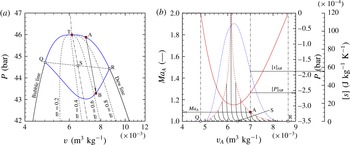
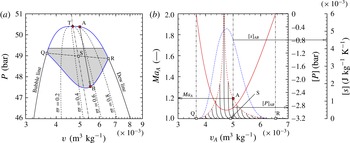
(a) The region bounded by the blue lines illustrates the thermodynamic domain in methane in which pure rarefaction shock waves can exist. Pre-shock states are in the negative-
 ${\it\Gamma}$
region. Also shown is an example of a condensation shock wave A–B featuring supersonic-to-sonic speed transition. State A is positioned near the dew line in the limit of
 ${\it\varpi}\uparrow 1$
, and state B is located in the VLE region characterized by
 ${\it\Gamma}>0$
. The low-pressure bound, i.e. the curve passing through points Q, B and R features post-shock sonic speeds for pre-shock states in close proximity to the saturation lines (on the bubble-line side,
 ${\it\varpi}\downarrow 0$
, and on the dew-line side,
 ${\it\varpi}\uparrow 1$
). The dash-dotted line through points T and S, respectively located on the bubble line and the
 ${\it\Gamma}=0$
line, represents an isentrope (here the choice is that
 $s$
is to the left of
 $s_{C}$
). (b) The pre-shock Mach number,
 $Ma_{A}$
, associated with a post-shock Mach number of unity, as a function of the pre-shock specific volume along selected isentropes (these are the black continuous lines; a special projection of figure 7 from the right-hand side) traversing the thermodynamic domain featuring
 ${\it\Gamma}<0$
. The
 $Ma_{A}$
versus
 $v_{A}$
lines of constant entropy start at the
 ${\it\Gamma}=0$
and terminate at very close proximity to the saturation lines. Rarefaction shock waves originating at these states, i.e. in the limit that the
 ${\it\varpi}$
approaches unity on the dew-line side and zero on the bubble-line side, feature the largest value of the wave Mach number. In the graph above, these states are connected with the red dashed lines. Additionally, for maximum Mach shocks (red dashed line), the continuous red line represents the pressure jump across the wave, and the blue dashed-dotted line illustrates the associated entropy increase across the wave. The fluid is methane and thermodynamic properties are determined with the EoS of Kurumov et al. (Reference Kurumov, Olchowy and Sengers1988). Also jump conditions for the exemplified shock wave A–B are shown.

In the present section, the admissibility region of pure, i.e. not composite, rarefaction shock waves is now identified. The procedure to compute the admissibility region is now detailed with the aid of figure 8 for methane fluid as follows:
-
(1) For the selected substance, draw on a
$P$
–
$v$
diagram the saturation and the
${\it\Gamma}=0$
curves. -
(2) Determine the values of the minimum and maximum entropy at points Q and R, respectively. Points Q and R are located on the
${\it\Gamma}=0$
line traversing the VLE region in the limit of the vapour mass fraction
${\it\varpi}$
approaching 0 and 1, respectively. All isentropes
$s_{i}$
,
$s_{Q}<s_{i}<s_{R}$
display a finite domain of concavity in the two-phase near-critical region. -
(3) Compute and draw thermodynamic
$P$
–
$v$
states along an isentrope
$s_{i}$
(start, for example, at the left-most thermodynamic state indicated by tag Q). -
(4) For the selected isentrope
$s_{i}$
, starting from the
${\it\Gamma}=0$
line, note
$v_{A}$
, and determine and record the pre-shock Mach number
$Ma_{A}$
, associated with a post-shock Mach number of unity (
$Ma_{B}=1$
, see figure 7), using system (3.1)–(3.3) and exploiting the geometric arguments to discern admissible shock waves from inadmissible solutions (these correspond to conditions (3.5)–(3.6)). Also, compute and record the post-shock states
$(P_{B},v_{B})$
, the pressure jump
$[P]=P_{B}-P_{A}$
and entropy jump
$[s]=s_{B}-s_{A}$
across the shock wave.
$[P]$
must be less than or at most equal to 0 (the zero value is valid for pre-shock points Q and R), and
$[s]$
must be greater than or at least equal to zero (zero at Q and R). -
(5) Along the same isentrope decrease then
$v$
by a small arbitrarily selected
${\rm\Delta}v$
. -
(6) For this new possible pre-shock state, note the new value for
$v_{A}$
and determine the pre-shock Mach number,
$Ma_{A}$
, associated with a post-shock Mach number of unity (
$Ma_{B}=1$
), by solving system (3.1)–(3.3) and (3.5)–(3.6). Also, compute the pressure jump
$[P]$
and entropy jump
$[s]$
as well as the post-shock thermodynamic states.


The Mach locus of figure 7 is illustrated in figure 8 for methane fluid on a
 $Ma_{A}$
–
 $v_{A}$
graph, together with other Mach loci along isentropes
 $s_{i}$
,
 $s_{Q}<s_{i}<s_{R}$
, computed using the procedure (4)–(6), for CH
 $_{4}$
; these Mach loci are indicated by black lines. Note that all Mach loci originate at the
 ${\it\Gamma}=0$
line and terminate at states approaching infinitesimally the saturation lines. In figure 8(b), the origins of the Mach loci are on the abscissa (see the position of point S), whereas the end points are connected by the maximum Mach curve: this curve connects states admitting rarefaction shock waves characterized by the greatest supersonic-to-sonic speed transition, as well as by the greatest jump in pressure for a given pre-shock state. The maximum Mach curve is the red dashed curve in figure 8(b). The locus of pre-shock states follows the contour of the saturation lines between points Q and R, whereby the post-shock states are located on curve Q–B–R, see figure 8(a). Also, the results of calculations yield that sonic post-shock states associated with pre-shock states that have been maximized, are located on a locus forming the low-pressure bound of the domain of existence of pure rarefaction shock waves. Furthermore, the locus of pre-shock states delimits the upper pressure boundary of the domain of admissibility of rarefaction shock waves. This locus of pre-shock states is located in close proximity to the saturation lines in the limit of the vapour mass fraction approaching zero on the bubble-line side, and one on the dew-line side. Only very close to the critical point the admissibility domain extends slightly into the single-phase region; this not visible in figure 8(a). The latter is elucidated near the end of this section.
In the case of methane shown in figure 8, the domain of validity of the scaled fundamental EoS encloses the region of negative nonlinearity and the admissibility domain of rarefaction shock waves. This however is not the case for carbon dioxide and ethylene. It is therefore necessary to assess if extrapolation of the EoS yields qualitatively and quantitatively satisfactory results for technical applications and analyses.
The following discusses to what extent the scaled EoS can be extended into the region sufficiently far from the critical point where mean field theory works (meaning, classical EoS can be used). That is to say, an assessment is made of quantifying what sufficiently far means. For this purpose experimental data for ethylene (Nehzat, Hall & Eubank Reference Nehzat, Hall and Eubank1983; Nowak, Kleinrahm & Wagner Reference Nowak, Kleinrahm and Wagner1996) and carbon dioxide (Duschek, Kleinrahm & Wagner Reference Duschek, Kleinrahm and Wagner1990), namely the isochoric heat capacity, the thermodynamic speed of sound, the saturation pressure and the saturated vapour density, are used. Here only the ethylene case is discussed in detail, as application of the same procedure to carbon dioxide leads to similar results. Note that the validity domain of the EoS as it is expressed by Sengers et al. (Reference Sengers, Greer and Sengers1976), in terms of density and temperature, viz.
 $279.00~\text{K}\leqslant T\leqslant 300.05~\text{K}$
and
 $160.62~\text{kg}~\text{m}^{-3}\leqslant {\it\rho}\leqslant 295.55~\text{kg}~\text{m}^{-3}$
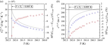
, respectively, is depicted in figure 2 by the region marked with the blue continuous lines. This figure shows that the computed region of negative nonlinearity, and consequently the admissibility domain of rarefaction shock waves, are located partly outside the reported validity domain; this situation is more pronounced on the vapour side of the VLE region (on the vapour side Senger’s EoS is valid only down to 281.4 K). In hindsight, since computations using the scaled fundamental EoS revealed that the lowest temperature of the computed admissibility domain of rarefaction shock waves corresponds to a temperature of 279.6 K, it became necessary to evaluate the effects of extrapolating primary and secondary property values obtained with the scaling laws along the dew line starting from
 $T_{C}$
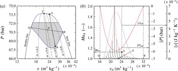
down to 279 K (the isochoric heat capacity and thermodynamic sound speed were only assessed down to 280.15 K, since a data survey conducted by the authors did not yield data at lower temperatures where scaling behaviour is still applicable). The conclusion of the assessment is that extrapolation predicts saturated densities, saturation pressures, isochoric heat capacities and thermodynamic sound speeds within 0.15 %, 0.019 %, 6 % and 7 % with respect to experimental data, respectively. It is noteworthy that, although the deviations of the calculated values with respect to experimental data are greater than the reported experimental uncertainties for quite a few data points, the values obtained from extrapolation are acceptable from the viewpoint of technical calculations. This statement can also be made by inspecting the observed trends showing monotonic changes in properties in the region of interest for extrapolation, as is expected and as is evident from figure 9(a,b). It may thus be stated with certainty that extrapolation down to 279 K is justified within the context and the the objectives of this work. The computed admissibility domains for rarefaction shock waves in ethylene and carbon dioxide, see figures 10 and 11, are thus at least qualitatively correct, as can also be argued based on the principle/law of corresponding states.
Comparison of saturated properties of ethylene obtained with the scaled fundamental EoS of Sengers et al. (Reference Sengers, Greer and Sengers1976) against experimental data from Nehzat et al. (Reference Nehzat, Hall and Eubank1983) for the isochoric heat capacity (a) and the thermodynamic speed of sound (b). The blue squares represent the actual data points, whereas the red squares denote the percentage deviations of the computed values with the EoS (dashed-dotted lines) with respect to the experimental values. The comparison shows that extrapolating properties using scaled equations slightly outside the stated validity range such that the treatment of non-classical gas dynamic phenomena in the vicinity of the vapour liquid critical point can be performed using one single thermodynamic model for the fluid does not appreciably affect the results from a technical point of view.

(a) Rarefaction shock wave admissibility domain of ethylene bounded by the blue continuous lines. The shaded area within the admissibility domain is the portion that falls outside the provided validity range of the scaled fundamental EoS used to compute the fluid properties. However, the outcome of an extensive validation with experimental data, justifies its use also for states lying in the shaded area as it ensures that the computed results are at least qualitatively correct. (b) Maximum Mach locus for ethylene. Refer to figure 8 for more details.

(a) Rarefaction shock wave admissibility domain of carbon dioxide bounded by the blue continuous lines. The shaded area within the admissibility domain is the portion that falls outside the provided validity range of the scaled fundamental EoS used to compute the fluid properties. However, the outcome of an extensive validation with experimental data, justifies its use also for states lying in the shaded area as it ensures that the computed results are at least qualitatively correct. (b) Maximum Mach locus for carbon dioxide. Refer to figure 8 for more details.

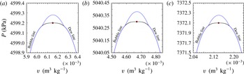
Admissibility domain in the very close proximity of the critical point of methane (CH
 $_{4}$
) (a), ethylene (C
 $_{2}$
H
 $_{4}$
) (b) and carbon dioxide (CO
 $_{2}$
) (c). From the blue line in the single-phase supercritical region double-sonic shocks are admissible.

In the very close proximity of the critical point, the slope of isentropic curves in the
 $P$
–
 $v$
plane becomes very small, due to the low values of the speed of sound in the near-critical region. Exactly at the critical point, the compressibility diverges and the critical isentrope exhibits a horizontal tangent. As a consequence, in a limited region in the very close proximity of the critical point, the single-phase speed of sound is lower than the speed of a finite-amplitude RSW in the two-phase region and therefore the admissibility region extends into the single-phase region. Since the slope of the isentropes decreases for fluid states located further away from the critical point in the single-phase region, double-sonic shocks are admissible for fluid states connecting the single-phase boundary of the admissibility region and its lower, two-phase boundary. The computed single-phase portion of the admissibility region is shown in figure 12, for methane, ethylene and carbon dioxide fluid. It is remarkable that for the three considered fluids, the single-phase admissibility region encompasses a very small range of pressures, which is of the order of millionths of the value of the critical pressure.
Note that the results presented here are valid under the assumption of thermodynamic equilibrium, which is acceptable since the shock waves considered are relatively thick and consequently the relaxation to thermal equilibrium takes place within the shock wave structure itself. For a particular shock wave in the critical region of methane the fluctuation spatial and time scale
 ${\it\xi}$
and
 ${\it\tau}$
have been estimated for the initial and the final states, respectively. For the post-shock final state,
 ${\it\tau}\approx 6\times 10^{-10}$
s. During this time, sound travels approximately
 $1.6\times 10^{-7}$
m. Therefore, the initial and final equilibrium states must be separated by a disturbed region at least that wide. For comparison, Borisov et al. (Reference Borisov, Kutateladze and Nakoryakov1983) computed a shock thickness of the order of cms for near-critical shock waves. The relatively large thickness is a consequence of the bulk viscosity being very large near the vapour–liquid critical point. The rarefaction shock wave in near-critical conditions may be influenced by critical point fluctuations. However, the pre- and post-shock states considered in the present work are located far enough from the critical point for fluctuations to be negligible.
6 Discussion and concluding remarks
The thermodynamic domain located near the vapour–liquid critical point of common fluids in which rarefaction shock waves can exists has been identified. For this purpose, a scaled fundamental EoS has been used, since it allows for the correct evaluation of the fluid thermodynamics in the domain of interest. For the considered exemplary fluids, namely methane, ethylene and carbon dioxide, the results indicate that pressure jumps as large as 6 bar with pre-shock Mach numbers between 1.5 and 2.0 are experimentally achievable.
An experiment to demonstrate the computed phenomenon appears to be feasible; however, provisions must be taken to limit gravity-induced density gradients from dehomogenizing the initial states. Even though the calculations are only conducted for three exemplary fluids, the predictions of these non-classical gas dynamic phenomena are universal: due to criticality the details of the system become irrelevant, and this behaviour must hold for all three-dimensional Ising-like systems. This is a major difference with the theory applicable to so-called BZT fluids, for which the possibility of non-classical phenomena depends on the molecular complexity of the substance being sufficiently large, and the thermal stability of the molecules sufficiently high, such that the molecules exist at the temperature at which these phenomena are predicted.
However, few caveats associated with the presented results are in order. Firstly, the models employed herein for methane, ethylene and carbon dioxide use critical exponents very close to the theoretical values. Therefore, it can be argued that the obtained results are generally valid in the near-critical vapour–liquid equilibrium region of any substance conforming to a so-called three-dimensional Ising-like system. Secondly, the situation here is that close to the critical point, the influence of surface tension on pressure reduces, because surface tension itself goes to low values and is zero at the critical point. Thirdly, the computed rarefaction shock waves will be dispersed due to phase transition; notwithstanding, the computed values of the pre- and post-shock states hold, under the condition that the predicted states are sufficiently far from the transition front.
Acknowledgements
This research has been partially supported by the Dutch Technology Foundation STW, Applied Science Division of NWO and the Technology Program of the Ministry of Economic Affairs, DSF 6573, and by the European Research Council under ERC Consolidator grant 2013, project NSHOCK 617603.