1 Introduction
Phoretic self-propulsion of catalytic colloids in an ambient solution is made possible by two independent physicochemical mechanisms: interfacial generation or consumption of solute molecules, and a short-range interaction of these molecules with the colloid boundary. If these mechanisms operate in an inhomogeneous fashion at the colloid boundary such that the solute–solid interaction acts in an asymmetric mode, the colloid may experience a net propulsive force. When the interaction potential is short range, it may be conveniently captured using an effective diffusio-osmotic slip (Anderson Reference Anderson1989). The first model of continuum self-diffusiophoresis (Golestanian, Liverpool & Ajdari Reference Golestanian, Liverpool and Ajdari2007) postulated a prescribed distribution of solute flux, leading in turn to an inhomogeneous Neumann condition. Later models, which employ a kinetic description of the interfacial reaction (Córdova-Figueroa & Brady Reference Córdova-Figueroa and Brady2008; Ebbens et al.
Reference Ebbens, Tu, Howse and Golestanian2012; Michelin & Lauga Reference Michelin and Lauga2014), result in a Robin-type macroscale condition. In that condition, the ratio of the respective magnitudes of chemical reaction and diffusion is represented by the Damköhler number
 $Da$
.
Theoretical analyses of self-diffusiophoresis have typically involved highly symmetric particle shapes (e.g. spheres), where the asymmetry required for self-propulsion is provided by a non-uniform distribution of interfacial absorption. Alternatively, self-diffusiophoresis may also be realised with a uniform distribution of interfacial reaction, provided the particle shape is asymmetric (Shklyaev, Brady & Córdova-Figueroa Reference Shklyaev, Brady and Córdova-Figueroa2014). This idea was addressed by Michelin & Lauga (Reference Michelin and Lauga2015), who considered slightly deformed spheres. The recent slender-body analysis of Schnitzer & Yariv (Reference Schnitzer and Yariv2015) may also serve to illustrate self-propulsion of chemically homogeneous particles.
Chemically homogeneous spherical particles lack a preferred direction in space and cannot undergo conventional self-propulsion when suspended in an unbounded domain. (Incorporation of the nonlinear mechanism of solute advection may result in spontaneous locomotion of such particles in an arbitrary direction in space, see Michelin, Lauga & Bartolo Reference Michelin, Lauga and Bartolo2013.) In a particle suspension, interaction between non-identical isotropic particles may result in self-propulsion; this possibility was explored for both the case of chemically dissimilar spheres (Soto & Golestanian Reference Soto and Golestanian2014) and different-sized spheres (Michelin & Lauga Reference Michelin and Lauga2015). Another venue for self-propulsion of isotropic particles has to do with the presence of a nearby boundary, which provides the requisite asymmetry (Domínguez et al. Reference Domínguez, Malgaretti, Popescu and Dietrich2016). This mode of self-diffusiophoresis is addressed here for the case of an inert solid wall.
The effect of solid walls on self-diffusiophoresis has been studied intensively in recent years, both experimentally (Volpe et al. Reference Volpe, Buttinoni, Vogt, Kümmerer and Bechinger2011; Kreuter et al. Reference Kreuter, Siems, Nielaba, Leiderer and Erbe2013; Das et al. Reference Das, Garg, Campbell, Howse, Sen, Velegol, Golestanian and Ebbens2015; Brown et al. Reference Brown, Vladescu, Dawson, Vissers, Schwarz-Linek, Lintuvuori and Poon2016; Simmchen et al. Reference Simmchen, Katuri, Uspal, Popescu, Tasinkevych and Sanchez2016) and theoretically (Volpe et al. Reference Volpe, Buttinoni, Vogt, Kümmerer and Bechinger2011; Ibrahim & Liverpool Reference Ibrahim and Liverpool2015; Uspal et al. Reference Uspal, Popescu, Dietrich and Tasinkevych2015; Mozaffari et al. Reference Mozaffari, Sharifi-Mood, Koplik and Maldarelli2016; Uspal et al. Reference Uspal, Popescu, Dietrich and Tasinkevych2016); these studies, however, appear to be exclusively focused upon Janus-type spherical particles. As the self-propulsion problem for the case of a homogeneous spherical particle is significantly simpler, it is amenable to treatment by analytic methods which provide valuable insight into the mechanism of particle–wall interactions. I therefore believe it deserves special attention.
Self-diffusiophoresis of an isotropic particle due to the presence on a nearby solid wall was discussed in a recent communication (Yariv Reference Yariv2016b
), where both remote and near-contact interactions were addressed. While the calculation of remote interactions is straightforward, the near-contact geometry reveals an unconventional situation. Thus, while self-propulsion is dominated (at least for moderate reaction rates, defined more precisely below) by the slip associated with the solute-concentration profile in the narrow gap separating the particle from the wall, that profile cannot be uniquely determined for any non-zero value of
 $Da$
using a lubrication analysis in this region. Calculation of the leading-order particle–wall interaction accordingly requires consideration of solute transport outside the gap. This task is undertaken here using matched asymptotic expansions. This systematic procedure allows to uniquely determine the solute concentration in the narrow gap, the consequent excess-pressure distribution in that region and the velocity imparted upon the particle by that distribution.
The paper is arranged as follows. In the next section we outline the physical problem considered. The corresponding dimensionless formulation is presented in § 3, where the near-contact limit is subsequently introduced. In § 4 we consider the fixed-flux model, corresponding to
 $Da=0$
, where solute transport in the narrow gap in uniquely determined by a standard lubrication analysis. The fixed-rate problem is discussed in § 5, where solute transport is analysed in both the inner gap region and the surrounding outer region. The gap-scale flow is calculated in § 6, where we employ a unified methodology valid for both the fixed-flux and fixed-rate models. With that flow determined, the leading-order approximation for the self-propulsive velocity is evaluated. In § 7 we compare that approximation with the numerical results of Mozaffari et al. (Reference Mozaffari, Sharifi-Mood, Koplik and Maldarelli2016). Concluding remarks are given in § 8, together with future research directions.
2 Physical problem
A chemically reactive spherical particle (radius
 $a$
) is suspended in a solution (solute diffusivity
 $D$
, viscosity
 $\unicode[STIX]{x1D707}$
) at a distance
 $h$
from an adjacent chemically inert planar wall. The equilibrium solute concentration, at large distances from the particle, is denoted by
 $c_{\infty }$
. Solute transfer at the particle boundary is modelled using a first-order chemical reaction,
 $$\begin{eqnarray}\displaystyle \text{solute absorption (per unit area)}=k\times \text{local bulk value of solute concentration},\quad & & \displaystyle\end{eqnarray}$$
where the rate constant
 $k$
is assumed uniform. Relation (2.1) naturally provides the kinetic flux scale
 $j=kc_{\infty }$
which, when balanced with diffusion, gives the characteristic scale
 $$\begin{eqnarray}\displaystyle {\mathcal{C}}=\frac{aj}{D} & & \displaystyle\end{eqnarray}$$
for the excess solute concentration (relative to
 $c_{\infty }$
) around the sphere, as generated by interfacial reaction.
On the macroscale, the short-range interaction between the solute molecules and the particle results in an osmotic pressure within a narrow layer surrounding the particle boundary. Osmotic-pressure variations, associated with the generally non-uniform excess solute concentration, scale as the product of that concentration with the Boltzmann temperature
 $kT$
. With the characteristic range
 $l$
of the interaction potential being small compared with both
 $a$
and
 $h$
, these variations result in diffusio-osmotic slip that scales as the product of
 $l^{2}/\unicode[STIX]{x1D707}$
with the pressure gradients. It follows that
 $$\begin{eqnarray}\displaystyle \text{slip velocity}=b\times \text{surface gradient of solute concentration}, & & \displaystyle\end{eqnarray}$$
where
 $b$
is of order
 $kTl^{2}/\unicode[STIX]{x1D707}$
; repulsive (e.g. steric) interactions are associated with a positive value of
 $b$
, and vice versa. The resulting velocity scale is
 $$\begin{eqnarray}\displaystyle {\mathcal{U}}=\frac{bj}{D}. & & \displaystyle\end{eqnarray}$$
The generic diffusio-osmotic slip relation (2.3) is assumed to hold on both the particle (
 $b=b_{p}$
) and wall (
 $b=b_{w}$
), with the respective slip coefficients being assumed uniform.
For convenience we calculate the flow about a stationary particle. Once the resulting hydrodynamic force on such a particle is determined the associated velocity of a comparable freely suspended particle is readily obtained using the well-known mobility expressions for the motion of a sphere perpendicular to a solid wall.
3 Dimensionless formulation
We employ a dimensionless notation where all length variables are normalised by
 $a$
. We employ the cylindrical coordinates
 $(\unicode[STIX]{x1D70C},\unicode[STIX]{x1D719},z)$
with corresponding unit vectors
 $(\hat{\boldsymbol{e}}_{\unicode[STIX]{x1D70C}},\hat{\boldsymbol{e}}_{\unicode[STIX]{x1D719}},\hat{\boldsymbol{e}}_{z})$
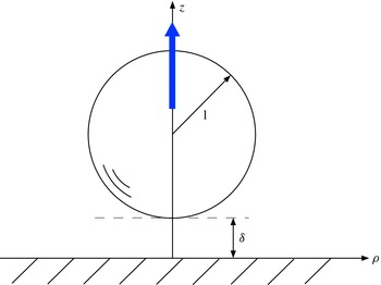
, see figure 1. The plane
 $z=0$
coincides with the fluid–wall interface while the
 $z$
-axis, which points into the fluid, passes through the particle centre. The azimuthal angle
 $\unicode[STIX]{x1D719}$
is degenerate in the axisymmetric problem considered.
Schematic of the dimensionless problem, indicating the particle autophoretic motion.

We employ the macroscale description of Michelin & Lauga (Reference Michelin and Lauga2014), neglecting however solute advection. The excess solute concentration
 $c$
, normalised by (2.2), is accordingly governed by: (i) Laplace’s equation; (ii) the no-flux condition at the inert wall,
 $$\begin{eqnarray}\displaystyle \frac{\unicode[STIX]{x2202}c}{\unicode[STIX]{x2202}z}=0\quad \text{at }z=0; & & \displaystyle\end{eqnarray}$$
(iii) the kinetic condition at the particle boundary,
 $$\begin{eqnarray}\displaystyle \frac{\unicode[STIX]{x2202}c}{\unicode[STIX]{x2202}n}=1+Da\,c, & & \displaystyle\end{eqnarray}$$
where
 $\unicode[STIX]{x2202}/\unicode[STIX]{x2202}n$
is a normal derivative into fluid and
 $Da=ka/D$
is the Damköhler number; and (iv) attenuation at large distances from the sphere,
 $$\begin{eqnarray}\displaystyle c\rightarrow 0\quad \text{as }\unicode[STIX]{x1D70C}^{2}+z^{2}\rightarrow \infty . & & \displaystyle\end{eqnarray}$$
In the reaction-limited case
 $Da=0$
condition (3.2) degenerates to that used in a fixed-flux description,
 $$\begin{eqnarray}\displaystyle \frac{\unicode[STIX]{x2202}c}{\unicode[STIX]{x2202}n}=1, & & \displaystyle\end{eqnarray}$$
corresponding to a uniformly prescribed inward solute flux of dimensional magnitude
 $j$
. While the fixed-rate condition (3.2) is meaningful only for literal absorption (
 $k>0$
), the degenerate fixed-flux condition (3.4) may be applied for both positive (consumption) and negative (production) values of
 $j$
(Michelin & Lauga Reference Michelin and Lauga2014).
The fluid velocity
 $\boldsymbol{u}=\hat{\boldsymbol{e}}_{\unicode[STIX]{x1D70C}}u+\hat{\boldsymbol{e}}_{z}w$
is normalised by (2.4) with
 $b=b_{p}+b_{w}$
. It is governed by: (i) the continuity and Stokes equations; (ii) far-field decay; and (iii) diffusio-osmotic slip (see (2.3))
 $$\begin{eqnarray}\displaystyle \boldsymbol{u}=\unicode[STIX]{x1D6FE}\unicode[STIX]{x1D735}_{s}c\quad \text{on the wall},\quad \boldsymbol{u}=(1-\unicode[STIX]{x1D6FE})\unicode[STIX]{x1D735}_{s}c\quad \text{on the particle}, & & \displaystyle\end{eqnarray}$$
where
 $\unicode[STIX]{x1D6FE}=b_{w}/(b_{w}+b_{p})$
and
 $\unicode[STIX]{x1D735}_{s}$
is the surface gradient. (Given (3.1), that operator degenerates into the conventional gradient in (3.5a
).)
By symmetry, the resulting hydrodynamic force (normalised by
 $\unicode[STIX]{x1D707}a{\mathcal{U}}$
) on the particle acts in the
 $z$
-direction, say
 $\hat{\boldsymbol{e}}_{z}f$
. The dimensionless force
 $f$
is a function of
 $Da$
and
 $\unicode[STIX]{x1D6FE}$
, as well as the single geometric parameter
 $\unicode[STIX]{x1D6FF}=h/a$
.
We focus upon the near-contact limit
 $\unicode[STIX]{x1D6FF}\ll 1$
. The gap region is described using the stretched cylindrical coordinates
 $$\begin{eqnarray}\displaystyle R=\unicode[STIX]{x1D70C}/\unicode[STIX]{x1D6FF}^{1/2},\quad Z=z/\unicode[STIX]{x1D6FF}. & & \displaystyle\end{eqnarray}$$
In these coordinates, the particle boundary in the gap region is given by
 $Z=H(R)+O(\unicode[STIX]{x1D6FF})$
where
 $H(R)=1+R^{2}/2$
.
4 Solute transport:
 $Da=0$

There is a fundamental difference in the analysis of the degenerated fixed-flux (
 $Da=0$
) problem and the general fixed-rate (
 $Da>0$
) one. The solution of the fixed-flux problem is provided in Yariv (Reference Yariv2016b
); as its details are required in § 5, it is briefly summarised here for completeness.
In the gap region we write
 $$\begin{eqnarray}\displaystyle c=C(R,Z;\unicode[STIX]{x1D6FF}), & & \displaystyle\end{eqnarray}$$
where
 $C$
satisfies Laplace’s equation,
 $$\begin{eqnarray}\displaystyle \frac{\unicode[STIX]{x2202}^{2}C}{\unicode[STIX]{x2202}Z^{2}}+\frac{\unicode[STIX]{x1D6FF}}{R}\frac{\unicode[STIX]{x2202}}{\unicode[STIX]{x2202}R}\left(R\frac{\unicode[STIX]{x2202}C}{\unicode[STIX]{x2202}R}\right)=0, & & \displaystyle\end{eqnarray}$$
the no-flux condition (cf. (3.1)),
 $$\begin{eqnarray}\displaystyle \frac{\unicode[STIX]{x2202}C}{\unicode[STIX]{x2202}Z}=0\quad \text{at }Z=0, & & \displaystyle\end{eqnarray}$$
and the prescribed-flux condition (cf. (3.4))
 $$\begin{eqnarray}\displaystyle \left(-\frac{\unicode[STIX]{x2202}C}{\unicode[STIX]{x2202}Z}+\unicode[STIX]{x1D6FF}R\frac{\unicode[STIX]{x2202}C}{\unicode[STIX]{x2202}R}\right)[1+O(\unicode[STIX]{x1D6FF})]=\unicode[STIX]{x1D6FF}\quad \text{at }Z=H(R)+O(\unicode[STIX]{x1D6FF}). & & \displaystyle\end{eqnarray}$$
Since (3.4) suggests an
 $O(1)$
excess concentration we postulate the asymptotic expansion
 $$\begin{eqnarray}\displaystyle C(R,Z;\unicode[STIX]{x1D6FF})=C_{0}(R,Z)+\unicode[STIX]{x1D6FF}C_{1}(R,Z)+\cdots \,. & & \displaystyle\end{eqnarray}$$
The leading-order balances of (4.2)–(4.4) readily imply that
 $C_{0}$
is independent of
 $Z$
and is therefore a function of
 $R$
alone. The function
 $C_{0}(R)$
is found from solvability conditions at
 $O(\unicode[STIX]{x1D6FF})$
. Thus, a single integration of Laplace’s equation at that order in conjunction with the
 $O(\unicode[STIX]{x1D6FF})$
balances of (4.3)–(4.4) yields
 $$\begin{eqnarray}\displaystyle \frac{H(R)}{R}\frac{\text{d}}{\text{d}R}\left(R\frac{\text{d}C_{0}}{\text{d}R}\right)+R\frac{\text{d}C_{0}}{\text{d}R}=1, & & \displaystyle\end{eqnarray}$$
namely a first-order ordinary differential equation governing
 $\text{d}C_{0}/\text{d}R$
. The solution of (4.6) which is regular at
 $R=0$
is
 $$\begin{eqnarray}\displaystyle \frac{\text{d}C_{0}}{\text{d}R}=\frac{R}{2H(R)}. & & \displaystyle\end{eqnarray}$$
Since diffusio-osmotic slip depends only upon solute-concentration gradients, no need arises to integrate this equation.
5 Solute transport:
$Da>0$

5.1 Gap-scale analysis
In analysing solute transport in the gap for the fixed-rate model, (3.2) suggests writing (cf. (4.1))
 $$\begin{eqnarray}\displaystyle c=-\frac{1}{Da}+C(R,Z;\unicode[STIX]{x1D6FF}). & & \displaystyle\end{eqnarray}$$
As in the case
 $Da=0$
,
 $C$
satisfies (4.2)–(4.3). Condition (4.4), however, is replaced by
 $$\begin{eqnarray}\displaystyle \left(-\frac{\unicode[STIX]{x2202}C}{\unicode[STIX]{x2202}Z}+\unicode[STIX]{x1D6FF}R\frac{\unicode[STIX]{x2202}C}{\unicode[STIX]{x2202}R}\right)[1+O(\unicode[STIX]{x1D6FF})]=\unicode[STIX]{x1D6FF}DaC\quad \text{at }Z=H(R)+O(\unicode[STIX]{x1D6FF}). & & \displaystyle\end{eqnarray}$$
In contrast with the case
 $Da=0$
the problem governing
 $C$
here is a homogeneous one. (In principle, the far-field decay (3.3) provides an inhomogeneous constraint on
 $C$
. That condition, however, does not apply in the gap region.) The asymptotic scaling of
 $C$
within the gap, say
 $\unicode[STIX]{x1D712}(\unicode[STIX]{x1D6FF})$
, cannot be determined from the gap-scale analysis.
We accordingly write (cf. (4.5))
 $$\begin{eqnarray}\displaystyle C(R,Z;\unicode[STIX]{x1D6FF})=\unicode[STIX]{x1D712}(\unicode[STIX]{x1D6FF})[C_{0}(R,Z)+\unicode[STIX]{x1D6FF}C_{1}(R,Z)+\cdots \,], & & \displaystyle\end{eqnarray}$$
and seek
 $C_{0}$
, postponing the determination of
 $\unicode[STIX]{x1D712}(\unicode[STIX]{x1D6FF})$
. Repeating the analysis of § 4 we again find from the leading-order balances that
 $C_{0}$
is independent of
 $Z$
with its dependence upon
 $R$
being determined from solvability conditions at
 $O(\unicode[STIX]{x1D6FF})$
. Here, the differential equation (4.6) is replaced by the homogeneous equation
 $$\begin{eqnarray}\displaystyle \frac{H(R)}{R}\frac{\text{d}}{\text{d}R}\left(R\frac{\text{d}C_{0}}{\text{d}R}\right)+R\frac{\text{d}C_{0}}{\text{d}R}-DaC_{0}=0. & & \displaystyle\end{eqnarray}$$
One of the solutions of (5.4) is (Kamke Reference Kamke2013)
 $$\begin{eqnarray}\displaystyle C^{(1)}(R)=\text{}_{2}F_{1}\left(\frac{1-\unicode[STIX]{x1D6FD}}{2},\frac{1+\unicode[STIX]{x1D6FD}}{2};1;-\frac{R^{2}}{2}\right), & & \displaystyle\end{eqnarray}$$
where
 $\text{}_{2}F_{1}$
is the Gaussian hypergeometric function and
 $$\begin{eqnarray}\displaystyle \unicode[STIX]{x1D6FD}=\sqrt{1+2Da}. & & \displaystyle\end{eqnarray}$$
The other solution, say
 $C^{(2)}(R)$
, cannot be conveniently expressed in terms of known functions. Now, local analysis about the regular singular point
 $R=0$
reveals (Bender & Orszag Reference Bender and Orszag1978) that one of the solutions is regular while the other possesses there a
 $\log R$
singularity; since (5.5) is regular at
 $R=0$
,
 $C^{(2)}(R)$
must introduce the inadmissible logarithmic singularity at
 $R=0$
and is accordingly discarded. We conclude that
 $$\begin{eqnarray}\displaystyle C_{0}=MC^{(1)}(R). & & \displaystyle\end{eqnarray}$$
Both the integration constant
 $M$
and the pre-factor
 $\unicode[STIX]{x1D712}$
may only be obtained using matched asymptotic expansions, where the narrow gap constitutes the inner region. The preceding inner analysis is accordingly followed by a comparable analysis of the outer region. In preparation for asymptotic matching we employ the well-known properties of the hypergeometric functions (Lebedev Reference Lebedev1972) to obtain the large-
 $R$
approximation of (5.7):
 $$\begin{eqnarray}\displaystyle C_{0}\sim MR^{\unicode[STIX]{x1D6FD}-1}\frac{\unicode[STIX]{x1D6E4}(\unicode[STIX]{x1D6FD})}{2^{(\unicode[STIX]{x1D6FD}-1)/2}\left\{\unicode[STIX]{x1D6E4}\left(\displaystyle \frac{1+\unicode[STIX]{x1D6FD}}{2}\right)\right\}^{2}}\quad \text{for }R\gg 1, & & \displaystyle\end{eqnarray}$$
 $\unicode[STIX]{x1D6E4}$
being the Gamma function.
5.2 Outer analysis
In the near-contact limit the outer region corresponds to the particle scale, where at leading order it appears to be touching the wall. This geometry is naturally handled using tangent-sphere coordinate
 $(\unicode[STIX]{x1D709},\unicode[STIX]{x1D719},\unicode[STIX]{x1D702})$
, where
 $\unicode[STIX]{x1D709}$
and
 $\unicode[STIX]{x1D702}$
are defined by the relations (Jeffrey Reference Jeffrey1978)
 $$\begin{eqnarray}\displaystyle \unicode[STIX]{x1D70C}=\frac{2\unicode[STIX]{x1D702}}{\unicode[STIX]{x1D709}^{2}+\unicode[STIX]{x1D702}^{2}},\quad z=\frac{2\unicode[STIX]{x1D709}}{\unicode[STIX]{x1D709}^{2}+\unicode[STIX]{x1D702}^{2}}. & & \displaystyle\end{eqnarray}$$
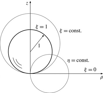
The coordinate surfaces are depicted in figure 2. The surfaces
 $\unicode[STIX]{x1D709}=\text{const.}$
are spheres of radius
 $1/\unicode[STIX]{x1D709}$
cantered about the point
 $\unicode[STIX]{x1D709}^{-1}\hat{\boldsymbol{e}}_{z}$
; the surfaces
 $\unicode[STIX]{x1D702}=\text{const.}$
are toroids of radius
 $1/\unicode[STIX]{x1D702}$
without centre opening. The wall is thus located at
 $\unicode[STIX]{x1D709}=0$
while the particle boundary is given to leading order by
 $\unicode[STIX]{x1D709}=1$
.
Tangent-sphere coordinates.

Since the imposed-rate condition (3.2) clearly implies that
 $c\sim O(1)$
, we write
 $$\begin{eqnarray}\displaystyle c(\unicode[STIX]{x1D709},\unicode[STIX]{x1D702};\unicode[STIX]{x1D6FF})\sim c_{0}(\unicode[STIX]{x1D709},\unicode[STIX]{x1D702})+\cdots \,, & & \displaystyle\end{eqnarray}$$
where the leading-order concentration
 $c_{0}$
satisfies Laplace’s equation, the boundary conditions (see (3.1)–(3.2))
 $$\begin{eqnarray}\displaystyle & \displaystyle \frac{\unicode[STIX]{x2202}c_{0}}{\unicode[STIX]{x2202}\unicode[STIX]{x1D709}}=0\quad \text{at }\unicode[STIX]{x1D709}=0, & \displaystyle\end{eqnarray}$$
 $$\begin{eqnarray}\displaystyle & \displaystyle \frac{\unicode[STIX]{x2202}c_{0}}{\unicode[STIX]{x2202}\unicode[STIX]{x1D709}}=-\frac{2}{1+\unicode[STIX]{x1D702}^{2}}-\frac{2Dac_{0}}{1+\unicode[STIX]{x1D702}^{2}}\quad \text{at }\unicode[STIX]{x1D709}=1, & \displaystyle\end{eqnarray}$$
and far-field decay
 $$\begin{eqnarray}\displaystyle c_{0}\rightarrow 0\quad \text{as }\unicode[STIX]{x1D709},\unicode[STIX]{x1D702}\rightarrow 0. & & \displaystyle\end{eqnarray}$$
Using the axisymmetric eigenfunctions of Laplace’s equation in tangent-sphere coordinates (see Moon & Spencer Reference Moon and Spencer1988) we find that the most general solution which satisfies conditions (5.11) and (5.13) is
 $$\begin{eqnarray}\displaystyle c_{0}=(\unicode[STIX]{x1D709}^{2}+\unicode[STIX]{x1D702}^{2})^{1/2}\int _{0}^{\infty }A(s)\cosh (\unicode[STIX]{x1D709}s)J_{0}(\unicode[STIX]{x1D702}s)\,\text{d}s. & & \displaystyle\end{eqnarray}$$
Substituting into (5.12) and making use of the well-known properties of the Hankel transform (Sneddon Reference Sneddon1972) yields the following second-order differential equation governing
 $A$
:
 $$\begin{eqnarray}\displaystyle s\sinh s\frac{\text{d}^{2}A}{\text{d}s^{2}}+(\sinh s+2s\cosh s)\frac{\text{d}A}{\text{d}s}-2DaA\cosh s=2\text{e}^{-s}. & & \displaystyle\end{eqnarray}$$
While the outer problem does not provide any boundary conditions to supplement this equation,
 $A$
may be obtained using the requirement of a convergent integral in (5.14), as detailed below.
Consider first the small-
 $s$
behaviour of
 $A$
. For
 $s\ll 1$
, (5.15) becomes
 $$\begin{eqnarray}\displaystyle & & \displaystyle s^{2}\left(1+\frac{s^{2}}{6}+\cdots \!\right)\frac{\text{d}^{2}A}{\text{d}s^{2}}+3s\left(1+\frac{7s^{2}}{18}+\cdots \!\right)\frac{\text{d}A}{\text{d}s}-2Da\left(1+\frac{s^{2}}{2}+\cdots \!\right)A\nonumber\\ \displaystyle & & \displaystyle \quad =2(1-s+\cdots \,).\end{eqnarray}$$
A particular solution of (5.16) is readily obtained as a power series
 $$\begin{eqnarray}\displaystyle -\frac{1}{Da}+\frac{2}{2Da-3}s+\cdots \,. & & \displaystyle\end{eqnarray}$$
(The apparent singularity at
 $Da=3/2$
indicates a transition at
 $\unicode[STIX]{x1D6FD}=2$
, see indeed (5.18).) Since
 $s=0$
is a regular singular point of the associated homogeneous equation, the complementary solutions behave there as
 $s^{-1\pm \unicode[STIX]{x1D6FD}}$
. To ensure small-
 $s$
convergence of the integral in (5.14) only the solution which behaves as
 $s^{\unicode[STIX]{x1D6FD}-1}$
is retained. We conclude that near
 $s=0$
the leading-order deviation from
 $-1/Da$
depends upon
 $\unicode[STIX]{x1D6FD}$
as follows:
 $$\begin{eqnarray}\displaystyle A(s)+\frac{1}{Da}\sim \left\{\begin{array}{@{}ll@{}}\displaystyle Ns^{\unicode[STIX]{x1D6FD}-1}+O(s), & \unicode[STIX]{x1D6FD}<2,\\ \displaystyle \frac{2}{2Da-3}s+Ns^{\unicode[STIX]{x1D6FD}-1}+O(s^{2}), & \unicode[STIX]{x1D6FD}>2,\end{array}\right. & & \displaystyle\end{eqnarray}$$
where
 $N$
is a constant.
Consider now large
 $s$
, where (5.15) becomes
 $$\begin{eqnarray}\displaystyle \frac{\text{d}^{2}A}{\text{d}s^{2}}+2\frac{\text{d}A}{\text{d}s}-\frac{2Da}{s}A\sim 4\frac{\text{e}^{-2s}}{s}. & & \displaystyle\end{eqnarray}$$
A particular solution of (5.19) is
 ${\sim}-2\text{e}^{-2s}/Da$
at large
 $s$
. Since
 $s=\infty$
is an irregular singular point of the associated homogeneous equation, the two complementary solutions of (5.19) behave there as a constant and
 $s^{Da}$
, respectively; because of the need for the integral appearing in (5.14) to converge at large
 $s$
, both solutions must identically vanish. We conclude that
 $$\begin{eqnarray}\displaystyle A\sim -\frac{2\text{e}^{-2s}}{Da}+\cdots \quad \text{as }s\rightarrow \infty . & & \displaystyle\end{eqnarray}$$
The preceding analyses allows to obtain
 $A$
as a quadrature. Thus, we write
 $A$
in the form
 $$\begin{eqnarray}\displaystyle A(s)=A_{p}(s)+NA_{h}(s), & & \displaystyle\end{eqnarray}$$
where
 $A_{p}$
in a solution of the inhomogeneous equation (5.15) while
 $A_{h}$
is a solution of the associated homogeneous equation. In particular, we choose
 $A_{p}$
as the solution that behaves as (5.17) for small
 $s$
and
 $A_{h}$
as the solution that behaves there as
 $s^{\unicode[STIX]{x1D6FD}-1}$
. Both
 $A_{p}$
and
 $A_{h}$
are obtained via numerical integration of the appropriate differential equation where the pertinent small-
 $s$
behaviour is used to obtain the requisite initial conditions. The coefficient
 $N$
in (5.21) is then chosen so as to make that combination satisfy (5.20). Because of the dependence upon
 $Da$
of both equation (5.15) as well as the small- and large-
 $s$
approximations,
 $N$
is a function of that parameter.
5.3 Asymptotic matching
With the outer solution determined, we perform the requisite asymptotic matching. The inner limit of the outer solution is attained when
 $\unicode[STIX]{x1D702}\gg 1$
(see (5.9)), where the integral appearing in (5.14) is dominated by the small-
 $s$
behaviour of
 $A$
. Employing (5.18) we find that, for
 $\unicode[STIX]{x1D6FD}<2$
,
 $$\begin{eqnarray}\displaystyle c_{0}+\frac{1}{Da}\sim N\unicode[STIX]{x1D702}^{1-\unicode[STIX]{x1D6FD}}\frac{2^{\unicode[STIX]{x1D6FD}-1}\unicode[STIX]{x1D6E4}\left(\displaystyle \frac{\unicode[STIX]{x1D6FD}}{2}\right)}{\unicode[STIX]{x1D6E4}\left(\displaystyle 1-\frac{\unicode[STIX]{x1D6FD}}{2}\right)}\quad \text{for }\unicode[STIX]{x1D702}\gg 1. & & \displaystyle\end{eqnarray}$$
Remarkably, this approximation also applies for
 $\unicode[STIX]{x1D6FD}>2$
, as the contribution of the
 $O(s)$
term in (5.18) turns out subdominant. In the gap region, where
 $\unicode[STIX]{x1D70C}\gg z$
, we find from (3.6a
) and (5.9a
) that
 $\unicode[STIX]{x1D702}\sim 2\unicode[STIX]{x1D6FF}^{-1/2}R^{-1}$
. Comparing with the inner approximation, provided by (5.1), (5.3) and (5.8), we find the pre-factor to be
 $$\begin{eqnarray}\displaystyle \unicode[STIX]{x1D712}(\unicode[STIX]{x1D6FF})=\unicode[STIX]{x1D6FF}^{(\unicode[STIX]{x1D6FD}-1)/2}. & & \displaystyle\end{eqnarray}$$
(Note that
 $\unicode[STIX]{x1D712}(\unicode[STIX]{x1D6FF})$
approaches unity when
 $Da\rightarrow 0^{+}$
, as it should.) The above matching also provides the value of the integration constant appearing in (5.7)
 $$\begin{eqnarray}\displaystyle M=\frac{2^{(\unicode[STIX]{x1D6FD}-1)/2}\unicode[STIX]{x1D6E4}\left(\displaystyle \frac{\unicode[STIX]{x1D6FD}}{2}\right)\left\{\unicode[STIX]{x1D6E4}\left(\displaystyle \frac{1+\unicode[STIX]{x1D6FD}}{2}\right)\right\}^{2}}{\unicode[STIX]{x1D6E4}(\unicode[STIX]{x1D6FD})\unicode[STIX]{x1D6E4}\left(1-\displaystyle \frac{\unicode[STIX]{x1D6FD}}{2}\right)}N. & & \displaystyle\end{eqnarray}$$
6 Gap flow and hydrodynamic force
6.1 Scaling
Consider now the gap flow for
 $Da>0$
. Since the slip condition (3.5) is unaffected by the constant term in (5.1), it is evident that the radial velocity
 $u$
is of order
 $\unicode[STIX]{x1D712}(\unicode[STIX]{x1D6FF})\unicode[STIX]{x1D6FF}^{-1/2}$
. The Stokes equation in the radial direction then implies that the associated pressure is of order
 $\unicode[STIX]{x1D712}(\unicode[STIX]{x1D6FF})\unicode[STIX]{x1D6FF}^{-2}$
. By setting
 $\unicode[STIX]{x1D712}$
to unity these scalings also apply for the case
 $Da=0$
.
Given (5.23), the hydrodynamic force associated with the pressure exerted on the
 $O(\unicode[STIX]{x1D6FF})$
gap-portion area of the particle boundary is of order
 $\unicode[STIX]{x1D6FF}^{(\unicode[STIX]{x1D6FD}-3)/2}$
. For ‘moderate’ reaction,
 $Da<4$
, where (see (5.6))
 $$\begin{eqnarray}\displaystyle \unicode[STIX]{x1D6FD}<3 & & \displaystyle\end{eqnarray}$$
this force is asymptotically large, dominating the corresponding
 $O(1)$
contribution from the outer region. In what follows we focus upon the case where (6.1) is satisfied.
6.2 Lubrication analysis
We hereafter employ a unified formulation, valid for both
 $Da=0$
and
 $Da>0$
. In the gap we write
 $u=U(R,Z;\unicode[STIX]{x1D6FF})$
and
 $p=P(R,Z;\unicode[STIX]{x1D6FF})$
, where the above lubrication scalings suggest the expansions
 $$\begin{eqnarray}\displaystyle & \displaystyle U(R,z;\unicode[STIX]{x1D6FF})=\unicode[STIX]{x1D712}(\unicode[STIX]{x1D6FF})\unicode[STIX]{x1D6FF}^{-1/2}[U_{0}(R,Z)+O(\unicode[STIX]{x1D6FF})], & \displaystyle\end{eqnarray}$$
 $$\begin{eqnarray}\displaystyle & \displaystyle P(R,z;\unicode[STIX]{x1D6FF})=\unicode[STIX]{x1D712}(\unicode[STIX]{x1D6FF})\unicode[STIX]{x1D6FF}^{-2}[P_{0}(R,Z)+O(\unicode[STIX]{x1D6FF})]. & \displaystyle\end{eqnarray}$$
From the leading-order balance of the Stokes equation in the
 $z$
-direction we find that
 $P_{0}$
is independent of
 $Z$
and is accordingly a function of
 $R$
alone, say
 $P_{0}(R)$
. The leading-order balance of the Stokes equation in the radial direction then gives
 $$\begin{eqnarray}\displaystyle \frac{\text{d}P_{0}}{\text{d}R}=\frac{\unicode[STIX]{x2202}^{2}U_{0}}{\unicode[STIX]{x2202}Z^{2}}. & & \displaystyle\end{eqnarray}$$
Two successive integrations in conjunction with the slip conditions (cf. (3.5))
 $$\begin{eqnarray}\displaystyle U_{0}=\unicode[STIX]{x1D6FE}\frac{\text{d}C_{0}}{\text{d}R}\quad \text{at }Z=0,\quad U_{0}=(1-\unicode[STIX]{x1D6FE})\frac{\text{d}C_{0}}{\text{d}R}\quad \text{at }Z=H(R), & & \displaystyle\end{eqnarray}$$
readily yield
 $$\begin{eqnarray}\displaystyle U_{0}(R,Z)=\frac{Z^{2}}{2}\frac{\text{d}P_{0}}{\text{d}R}+\frac{Z}{H(R)}\left[(1-2\unicode[STIX]{x1D6FE})\frac{\text{d}C_{0}}{\text{d}R}-\frac{H^{2}(R)}{2}\frac{\text{d}P_{0}}{\text{d}R}\right]+\unicode[STIX]{x1D6FE}\frac{\text{d}C_{0}}{\text{d}R}. & & \displaystyle\end{eqnarray}$$
Applying the axisymmetric condition of zero net radial flux,
 $\int _{0}^{H(R)}U_{0}(R,Z)\,\text{d}Z=0$
, then yields the equation
 $$\begin{eqnarray}\displaystyle \frac{\text{d}P_{0}}{\text{d}R}=\frac{6}{H^{2}(R)}\frac{\text{d}C_{0}}{\text{d}R}. & & \displaystyle\end{eqnarray}$$
Because of the need for the
 $O(\unicode[STIX]{x1D6FF}^{(\unicode[STIX]{x1D6FD}-5)/2})$
gap pressure to match the
 $O(1)$
outer pressure, and given (6.1),
 $P_{0}$
must also satisfy the decay condition
 $$\begin{eqnarray}\displaystyle \lim _{R\rightarrow \infty }P_{0}=0. & & \displaystyle\end{eqnarray}$$
Integration of (6.7) thus furnishes the gap pressure,
 $$\begin{eqnarray}\displaystyle P_{0}(R)=-6\int _{R}^{\infty }\frac{\text{d}C_{0}}{\text{d}R^{\prime }}\frac{\text{d}R^{\prime }}{H^{2}(R^{\prime })}. & & \displaystyle\end{eqnarray}$$
Given (4.7) and (5.8),
 $P_{0}$
decays like
 $R^{\unicode[STIX]{x1D6FD}-5}$
at large
 $R$
. Note that
 $P_{0}$
is independent of
 $\unicode[STIX]{x1D6FE}$
; in view of the normalisation by
 $b_{p}+b_{w}$
, this independence implies a dimensional repulsion that depends on the slip coefficients only through their sum.
6.3 Hydrodynamic force
Given the preceding arguments, the hydrodynamic force
 $f$
exerted on the particle is written as
 $$\begin{eqnarray}\displaystyle \unicode[STIX]{x1D6FF}^{(\unicode[STIX]{x1D6FD}-3)/2}F_{0}+\cdots \,, & & \displaystyle\end{eqnarray}$$
where
 $F_{0}$
is contributed by the gap pressure:
 $$\begin{eqnarray}\displaystyle F_{0}=2\unicode[STIX]{x03C0}\int _{0}^{\infty }RP_{0}(R)\,\text{d}R. & & \displaystyle\end{eqnarray}$$
(As expected, the integral converges at large
 $R$
if and only if (6.1) is satisfied.) Substituting (6.9) and replacing the order of integration gives
 $F_{0}=-6\unicode[STIX]{x03C0}{\mathcal{F}}$
where
 $$\begin{eqnarray}\displaystyle {\mathcal{F}}=\int _{0}^{\infty }\frac{R^{2}}{H^{2}(R)}\frac{\text{d}C_{0}}{\text{d}R}\,\text{d}R. & & \displaystyle\end{eqnarray}$$
For
 $Da=0$
, substitution of (4.7) yields
 $$\begin{eqnarray}\displaystyle {\mathcal{F}}={\textstyle \frac{1}{2}}. & & \displaystyle\end{eqnarray}$$
For
 $Da>0$
we obtain the scaled force
 ${\mathcal{F}}$
by substituting (5.7), with
 $M$
provided by (5.24), into (6.12). The force depends upon
 $Da$
explicitly, through both (5.7) and (5.24), and implicitly, through the value of
 $N$
(see (5.21) et seq.).
We have applied the procedure outlined in § 5.2 to calculate
 $N$
, the coefficient appearing in (5.21), up to approximately
 $Da=1.8$
, at which value further calculations have become challenging. The resulting dependence of
 ${\mathcal{F}}$
upon
 $Da$
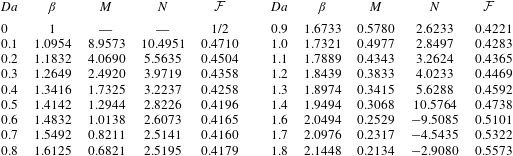
is illustrated in table 1. This table portrays a non-monotonic variation, with
 ${\mathcal{F}}$
initially decreasing from (6.13), reaching a minimum around
 $Da=0.7$
, and then increasing with
 $Da$
. Note the singularity of
 $N$
around
 $Da=3/2$
, corresponding to the transition at
 $\unicode[STIX]{x1D6FD}=2$
between the two branches of (5.18). This singularity does not affect the monotonic increase of
 ${\mathcal{F}}$
with
 $Da$
.
The force coefficient
 ${\mathcal{F}}$
as a function of
 $Da$
. For any given value of
 $Da$
, the coefficient
 $N$
appearing in (5.21) is determined using the procedure outlined in § 5.2. The coefficient
 $M$
in (5.7) is then obtained from (5.24), and the force
 ${\mathcal{F}}$
is calculated using quadrature (6.12).

6.4 Particle speed
Having calculated the hydrodynamic force we readily obtain the velocity acquired by a freely suspended particle. For
 $\unicode[STIX]{x1D6FF}\ll 1$
, the mobility coefficient associated with motion of a sphere perpendicular to a solid wall is
 $\unicode[STIX]{x1D6FF}/6\unicode[STIX]{x03C0}$
at leading order (Cox & Brenner Reference Cox and Brenner1967). Using (6.10), the velocity imparted to the swimmer in the negative
 $z$
-direction is
 $$\begin{eqnarray}\displaystyle \unicode[STIX]{x1D6FF}^{(\unicode[STIX]{x1D6FD}-1)/2}{\mathcal{F}}+\cdots \,. & & \displaystyle\end{eqnarray}$$
For
 $Da=0$
the phoretic velocity approaches a finite value as
 $\unicode[STIX]{x1D6FF}\rightarrow 0$
. For
 $0<Da<4$
, where
 $\unicode[STIX]{x1D6FF}\ll \unicode[STIX]{x1D712}\ll 1$
, the particle velocity scales as an irrational positive power of
 $\unicode[STIX]{x1D6FF}$
. For strong kinetics,
 $Da>4$
,
 $\unicode[STIX]{x1D712}\ll \unicode[STIX]{x1D6FF}$
. The hydrodynamic force on a stationary particle is dominated by the outer contribution and is accordingly
 $O(1)$
. The corresponding velocity of a freely suspended particle thus remains at
 $O(\unicode[STIX]{x1D6FF})$
. The case
 $Da=4$
(
 $\unicode[STIX]{x1D712}=\unicode[STIX]{x1D6FF}$
) is a borderline one where the hydrodynamic force is expected to scale as
 $\log \unicode[STIX]{x1D6FF}$
(Yariv Reference Yariv2016a
).
7 Comparison with Mozaffari et al. (Reference Mozaffari, Sharifi-Mood, Koplik and Maldarelli2016)
In their paper, Mozaffari et al. (Reference Mozaffari, Sharifi-Mood, Koplik and Maldarelli2016) considered the motion of a spherical locomotor in the vicinity of an inert wall. Their geometry is more complicated than the one analysed herein, as it entails a compound spherical particle, consisting of a catalyst cap on which solute is produced and an inert part. The boundary condition employed on the catalyst cap specifies a uniform flux, similar (up to a sign difference) to (3.4). Considering the general case of arbitrary particle–wall separations, Mozaffari et al. (Reference Mozaffari, Sharifi-Mood, Koplik and Maldarelli2016) utilised bi-spherical coordinates to analyse the solute transport and flow problems, employing the familiar eigenfunctions of the respective Laplace and Stokes equations in these coordinates; the associated series solutions for the colloid velocity were then numerically evaluated. The smallest value of the dimensionless gap thickness
 $\unicode[STIX]{x1D6FF}$
for which results were presented is about
 $0.01$
. These results have been obtained for various values of
 $\unicode[STIX]{x1D703}_{cap}$
, the catalytic cap polar angle measured from the swimmer axis (
 $\unicode[STIX]{x1D703}_{cap}=90^{\circ }$
corresponding to a Janus particle), and
 $\unicode[STIX]{x1D6EF}$
, the particle tilt relative to the wall (
 $\unicode[STIX]{x1D6EF}=0$
corresponding to the cap facing the wall).
A key observation in the present small-
 $\unicode[STIX]{x1D6FF}$
analysis is that, in the fixed-flux model, self-propulsion is dominated by the gap-scale transport. It is evident that this asymptotic dominance is retained even if one were to consider the compound geometry of Mozaffari et al. (Reference Mozaffari, Sharifi-Mood, Koplik and Maldarelli2016), provided the cap size is large enough so that the gap is bounded by the cap area of the colloid. In fact, said dominance holds even in non-axisymmetric configurations, where the particle axis is tilted relative to the vertical, as long as the tilt angle is sufficiently smaller than the cap angle. We therefore expect that for small
 $\unicode[STIX]{x1D6FF}$
the numerical results of Mozaffari et al. (Reference Mozaffari, Sharifi-Mood, Koplik and Maldarelli2016) would agree with our prediction of
 $1/2$
dimensionless speed, see (6.13) and (6.14).
This is indeed the case. Figure 12(b) of Mozaffari et al. (Reference Mozaffari, Sharifi-Mood, Koplik and Maldarelli2016) presents the colloid speed perpendicular to the wall as a function of
 $\unicode[STIX]{x1D6FF}$
for
 $\unicode[STIX]{x1D703}_{cap}=150^{\circ }$
and several values of
 $\unicode[STIX]{x1D6EF}$
. Extrapolation of the curves appearing in that figure indicates that this velocity approaches a finite value as
 $\unicode[STIX]{x1D6FF}$
becomes small, the value being the same for tilt angles
 $\unicode[STIX]{x1D6EF}=60^{\circ }$
,
 $90^{\circ }$
and
 $120^{\circ }$
. As these values are sufficiently smaller than
 $\unicode[STIX]{x1D703}_{cap}$
the active area of the particle faces the wall in the gap region. Considering the different velocity scale used in the normalisation process (see equation (2) of Mozaffari et al.
Reference Mozaffari, Sharifi-Mood, Koplik and Maldarelli2016), that value indeed agrees with the
 $1/2$
value obtained in the present analysis. (As Mozaffari et al.
Reference Mozaffari, Sharifi-Mood, Koplik and Maldarelli2016 assume solute absorption, they predict particle motion away from the wall.) The same agreement is observed in figure 10(a) of Mozaffari et al. (Reference Mozaffari, Sharifi-Mood, Koplik and Maldarelli2016) where the particle speed is presented for
 $\unicode[STIX]{x1D703}_{cap}=120^{\circ }$
; here the limiting behaviour holds for a smaller range of tilt angles, in agreement with the preceding discussion.
8 Concluding remarks
We have analysed the boundary-induced autophoresis of an isotropic colloid. Focusing upon the near-contact limit we have obtained the leading-order approximation (6.14) for the particle velocity perpendicular to the wall. Our results are valid for moderate reaction rates,
 $Da<4$
, predicting dimensionless velocities that scale as
 $\unicode[STIX]{x1D6FF}^{(\sqrt{1+2Da}-1)/2}$
. Beyond this value the particle velocity is
 $O(\unicode[STIX]{x1D6FF})$
, determined by stresses in the outer region. The degenerate case
 $Da=0$
, where the velocity is
 $O(1)$
, corresponds to a prescribed-flux boundary condition.
Going back to dimensional notation, we see that the particle moves into the wall with the velocity
 $$\begin{eqnarray}\displaystyle {\mathcal{F}}\frac{(b_{p}+b_{w})kc_{\infty }}{D}\left(\frac{h}{a}\right)^{(\sqrt{1+2ka/D}-1)/2}, & & \displaystyle\end{eqnarray}$$
where the dependence of
 ${\mathcal{F}}$
upon the Damköhler number
 $ka/D$
is provided in table 1. While the generic velocity scale (2.4) is independent of
 $a$
, the near-contact limit (8.1) involves a rather anomalous dependence upon particle size. The appropriate dimensional expression for the prescribed-flux problem, corresponding to a uniform inward solute flux of magnitude
 $j$
, is (see (6.13))
 $$\begin{eqnarray}\displaystyle \frac{(b_{p}+b_{w})j}{2D}. & & \displaystyle\end{eqnarray}$$
Future investigations of the present particle–wall interaction problem with the fixed-rate model may address the general case of arbitrary separations, where
 $\unicode[STIX]{x1D6FF}=O(1)$
, using spherical bipolar coordinates. Since the remote interaction limit has already predicted dimensionless velocities which, in the present notation, depend upon
 $\unicode[STIX]{x1D6FE}$
(Yariv Reference Yariv2016b
), that dependence must also appear in the general case
 $\unicode[STIX]{x1D6FF}=O(1)$
. The simple proportionality of the dimensional velocity (8.1) in the sum of the slip coefficients is therefore restricted to the near-contact limit.
A different venue involves compound (e.g. Janus) particles, such as those considered by Mozaffari et al. (Reference Mozaffari, Sharifi-Mood, Koplik and Maldarelli2016). It was observed in § 7 that the leading-order particle–wall repulsion predicted by the present asymptotic analysis also applies to those compound particles, even in non-axisymmetric configurations, provided the active cap area faces the wall in the gap region. For non-zero tilt angles, where the problem does not possess axial symmetry, the particle also acquires a velocity parallel to the wall. It is evident that this motion is dominated by the
 $O(1)$
stresses in the outer region. The associated mobility as
 $\unicode[STIX]{x1D6FF}\rightarrow 0$
is however of order
 $1/\text{log}\unicode[STIX]{x1D6FF}$
(Goldman, Cox & Brenner Reference Goldman, Cox and Brenner1967), asymptotically larger than the
 $O(\unicode[STIX]{x1D6FF})$
mobility perpendicular to the wall. Considering logarithmic terms on par with
 $O(1)$
terms (Hinch Reference Hinch1991) we practically expect
 $O(1)$
particle velocities parallel to the wall for small values of
 $\unicode[STIX]{x1D6FF}$
. This is indeed observed in both figures 10(b) and 12(c) in Mozaffari et al. (Reference Mozaffari, Sharifi-Mood, Koplik and Maldarelli2016). These
 $O(1)$
velocities may be determined, in principle, by extending the present analysis to non-axisymmetric configurations. Given the difficulty to obtain converging numerical solutions at small values of
 $\unicode[STIX]{x1D6FF}$
, it is challenging to infer the small-
 $\unicode[STIX]{x1D6FF}$
limit of the particle velocities from these solutions (as is evident from the figures of Mozaffari et al.
Reference Mozaffari, Sharifi-Mood, Koplik and Maldarelli2016). The asymptotic extension suggested here would accordingly complement the bipolar-coordinate solutions.
Acknowledgements
I am grateful to the anonymous referee for pointing out the applicability of the present approximation to compound particles, leading in turn to § 7. This work was supported by the Israel Science Foundation (grant no. 1081/16).