




1. Introduction
Nonlinear waves in non-integrable Hamiltonian lattices, such as the celebrated Fermi–Pasta–Ulam (FPU) problem [Reference Fermi, Pasta and Ulam18] and its various extensions and physical applications, have attracted a lot of attention [Reference Chong and Kevrekidis7, Reference Flach and Gorbach20, Reference Kevrekidis27, Reference Pankov31, Reference Sen, Hong, Bang, Avalos and Doney34, Reference Vainchtein38]. The dynamics of these waves is very rich due to the combination of higher order dispersion intrinsic to the lattice setting and higher order nonlinearity that is often present in such models. In the absence of integrability, this combination makes the tools of Whitham modulation theory and more recent advances in dispersive hydrodynamics [Reference El and Hoefer16, Reference Kamchatnov25, Reference Whitham39] particularly promising for providing insight into the collective, multiscale dynamics of interacting lattice waves and for describing complex waveforms such as dispersive shock waves and travelling waves connecting periodic orbits. Some work in this direction has begun [Reference Dreyer and Herrmann11–Reference Dreyer, Herrmann and Rademacher13, Reference Filip and Venakides19, Reference Sprenger, Chong, Okyere, Herrmann, Kevrekidis and Hoefer35, Reference Yang, Biondini, Chong and Kevrekidis40] but much remains to be investigated.
A fundamental concept of primary importance for lattice dispersive hydrodynamics is the hyperbolicity of the modulation equations for the FPU problem. Hyperbolicity governs the dynamical stability and structure of multiscale wave dynamics [Reference Whitham39]. In the non-integrable FPU problem, hyperbolicity has only been assessed in some special limits, such as the harmonic chain, the hard-sphere model and small-amplitude periodic travelling waves [Reference Dreyer, Herrmann and Mielke12]. Another related concept for a hyperbolic system is that of a genuinely nonlinear characteristic field [Reference Lax29], which is a necessary condition for the construction of simple waves (integral curves) that form the foundation for solutions to Riemann problems and dispersive shock waves [Reference El and Hoefer16]. We say that a hydrodynamic-type system of Whitham modulation equations is convex if it is strictly hyperbolic and genuinely nonlinear [Reference Levermore30]. A modulation system may be convex for a restricted subset of the state variables.
The present work focuses on studying the modulation system and its convexity for the modified regularized Boussinesq equation, a non-integrable dispersive partial differential equation that approximates FPU dynamics [Reference Rosenau33]. The regularized Boussinesq equation has been shown to capture some FPU features, including travelling kink fronts, solitary waves and dispersive shocks [Reference Vainchtein and Truskinovsky36, Reference Yang, Biondini, Chong and Kevrekidis40]. We consider a general cubic nonlinearity that enables construction of explicit periodic travelling waves in terms of elliptic functions and systematically investigate all of the different cases and special limits. While it is typically assumed that all of the roots of the polynomial determining periodic travelling waves are real, our analysis includes the case when two of the roots become complex, which is relevant for the nonlinear interaction force with positive cubic-term coefficient. The transition from real to complex roots involves a bifurcation where the solution is a trigonometric wave. We then proceed to derive the Whitham modulation equations using Whitham’s averaged variational principle [Reference Kamchatnov25, Reference Whitham39] and discuss their structure for three distinct cases: i) quadratic nonlinearity 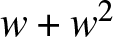 $w+w^2$ and cubic nonlinearities ii)
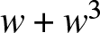 $w+w^3$, iii)
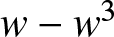 $w-w^3$. The cubic cases correspond to a nonconvex hyperbolic flux. We also discuss the reduction of these equations in the harmonic and solitary-wave limits. In the case of
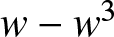 $w-w^3$, we obtain the wave-action conservation law for the kink limit, which yields a non-classical, undercompressive shock [Reference El, Hoefer and Shearer17, Reference Herrmann and Rademacher23], or superkink [Reference Gorbushin, Vainchtein and Truskinovsky22].
The main part of the paper focuses on determining the regions of convexity for the Whitham system where it is strictly hyperbolic and genuinely nonlinear. In the harmonic and solitary-wave limits, the convexity is examined analytically, and the full Whitham system is studied numerically. In each case, we identify parameterizations that allow us to present the results in a systematic way in terms of physically relevant parameters. In the case of quadratic nonlinearity, a symmetry of the governing equations enables a complete convexity characterization of the modulation system in terms of a two-dimensional parameter space. Meanwhile, in the cubic cases, a three-dimensional parameterization is needed, and we convey the results in a two-parameter plane for different values of the wave amplitude. The regions where hyperbolicity fails are indicated by contour plots of the imaginary part of the corresponding eigenvalue, while the loss of genuine nonlinearity is indicated by curves in the two-dimensional parameter plane.
Our results show that in the case of quadratic nonlinearity, the Whitham system is convex, i.e., strictly hyperbolic and genuinely nonlinear, for sufficiently small amplitude and sufficiently large mean strain. In the real-root case for nonlinearity 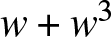 $w+w^3$, our computations suggest strict hyperbolicity of the Whitham equations in the entire parameter range. However, the system loses genuine nonlinearity along two curves that bifurcate from the solitary-wave limit. The situation is different in the complex-root case, where we observe loss of hyperbolicity in an amplitude-dependent part of the parameter domain, as well as loss of genuine nonlinearity in up to three characteristic fields. As the amplitude is increased, the convexity domain becomes larger. In the case of cubic nonlinearity
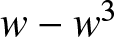 $w-w^3$, the convexity figures become even more complex. For a fixed amplitude, there are two domains where hyperbolicity is lost, including a parameter range in the solitary-wave limit, in addition to several curves marking the loss of genuine nonlinearity. The convexity domain is larger for smaller amplitudes in this case.
The loss of hyperbolicity is known to correspond to modulational instability [Reference Whitham39], and rigorously so in some specific cases [Reference Benzoni-Gavage, Noble and Rodrigues1, Reference Bronski and Johnson3, Reference Clarke, Marangell and Perkins8, Reference Johnson and Perkins24]. We verify the onset of modulational instability by numerically computing the spectrum of the linearized operator using the Floquet–Fourier–Hill method [Reference Deconinck and Kutz10] and show that the slopes of the associated cross structure in the spectrum near the origin are well approximated in terms of the real and imaginary parts of the Whitham characteristic velocities. In addition to confirming the emergence of modulational instability, our spectral calculations reveal short-wavelength instabilities in both modulationally stable and unstable cases, including superharmonic instabilities studied in detail in [Reference Bronski, Hur and Wester2] for the case of quadratic nonlinearity. We also conduct numerical simulations initiated by modulationally unstable periodic travelling waves perturbed by the corresponding unstable eigenmode. The results confirm the development of modulational instability along with short-wavelength instabilities that eventually lead to the blowup of the solution in some cases.
The rest of the paper is organized as follows. In Section 2, we introduce the quasicontinuum model and discuss parameter reduction, conservation laws and averaging. Explicit periodic travelling wave solutions, their harmonic, solitary-wave and kink limits, existence domain and parameterizations are discussed in Section 3. In Section 4, we derive the Whitham modulation equations and investigate their structure, special limits and convexity. In Section 5, we verify the onset of modulational instability and explore other instability modes by examining the spectra of the linearized operator and conducting numerical simulations. Concluding remarks are found in Section 6.
2. Preliminaries
2.1. Quasicontinuum model
We consider the dispersive quasicontinuum model (modified regularized Boussinesq equation)
 \begin{equation}
u_{tt}-\dfrac{1}{12}u_{xxtt}=(f(u_x))_x,
\end{equation}
which approximates the FPU problem
 \begin{equation}
\ddot{u}_n=f(u_{n+1}-u_n)-f(u_n-u_{n-1})
\end{equation}
for a chain of masses with displacements  $u_n(t)$ and interaction force
 $f(w)$. This can be shown [Reference Rosenau33] by rewriting (2.2) in terms of strain variables
 $w_n=u_n-u_{n-1}$, using a Padé approximation of the discrete operator and integrating the resulting PDE to obtain the displacement formulation (2.1). In what follows, we consider the cubic interaction force
 \begin{equation}
f(w)=w+\alpha w^2+\beta w^3,
\end{equation}
which corresponds to the  $\alpha$-
 $\beta$-FPU problem (2.2).
Observe that if 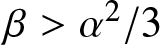 $\beta \gt \alpha^2/3$ or
 $\beta \lt 0$, the change of variables
 \begin{equation*}
u(x,t) = \left ( 1-\frac{\alpha^2}{3\beta} \right )^{1/2} y(x,\tau) -
\frac{\alpha}{3\beta} x, \quad \tau =
\left ( 1-\frac{\alpha^2}{3\beta} \right )^{1/2}t,
\end{equation*}
yields the reduced equation
 \begin{equation*}
y_{\tau\tau} - y_{xx} - \beta\left (y_x^3 \right )_x -
\frac{1}{12} y_{xx\tau\tau} = 0
\end{equation*}
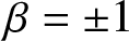
that involves no quadratic term in the interaction force. Because of this, we can, in the aforementioned regimes, set  $\alpha = 0$. The additional rescaling
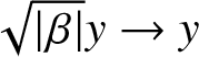 $\sqrt{|\beta|} y \to y$ allows one to take
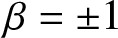 $\beta = \pm 1$ without loss of generality. Similarly, if
 $\beta=0$ but
 $\alpha$ is nonzero (quadratic interaction), the rescaling
 $\alpha u \to u$ means that we can set
 $\alpha = 1$. This change of variables is reminiscent of the transformation of solutions of the Gardner equation to solutions of the modified Korteweg-de Vries or Korteweg-de Vries equations [Reference Kamchatnov, Kuo, Lin, Horng, Gou, Clift, El and Grimshaw26]. In what follows, we will proceed with
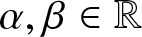 $\alpha,\beta \in \mathbb{R}$ and either
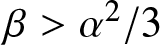 $\beta \gt \alpha^2/3$,
 $\beta \lt 0$, or
 $\beta = 0$ and then restrict to
 $\alpha = 0$,
 $\beta = \pm 1$ and
 $\alpha= 1$,
 $\beta=0$ when convenient.
Linearizing (2.1) about the uniformly deformed state by setting  $u(x,t) = x \overline{w} + \epsilon e^{i(kx-\omega_0t)}$ and taking the limit
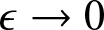 $\epsilon \to 0$, we obtain the linear dispersion relation
 \begin{align}
\omega_0^2(k,\overline{w}) = \frac{k^2 c_s^2(\overline{w})}{1+k^2/12} \lt 12 c_s^2(\overline{w}),
\end{align}
where
 \begin{align}
c_s(\overline{w})=(f'(\overline{w}))^{1/2}=(1+2\alpha \overline{w}+3\beta \overline{w}^2)^{1/2}
\end{align}
is the sound (long-wave) speed.
2.2. Conservation laws
Equation (2.1) corresponds to the Lagrangian density
 \begin{align}
\mathbb{L}=\dfrac{1}{2}v^2-\phi(w)+\dfrac{1}{24}w_t^2,
\end{align}
where 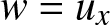 $w=u_x$ is the strain,
 $\phi(w)$ is the elastic energy density determining the force
 $f(w) = \phi'(w)$, and
 $v=u_t$ is the particle velocity. The regularized Boussinesq equation (2.1) can be written as the first-order system in conservative form
 \begin{align}
w_t - v_x = 0, \quad v_t-\left (f(w) + \dfrac{1}{12}w_{tt} \right )_x =0.
\end{align}
Translational invariance of  $\mathbb{L}$ implies two additional conservation laws that are equivalent for smooth solutions [Reference Gavrilyuk, Nkonga, Shyue and Truskinovsky21]. The first one is the energy balance,
 \begin{align}
\dfrac{\partial}{\partial
t}\left(\phi(w)+\dfrac{v^2}{2}+\dfrac{1}{24}w_t^2\right)-\dfrac{\partial}{\partial
x}\left[\left(f(w)+\dfrac{1}{12}w_{tt}\right)v\right]=0,
\end{align}
where 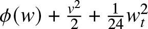 $\phi(w)+\frac{v^2}{2}+\frac{1}{24}w_t^2$ is the energy density, and
 $-(f(w)+\frac{1}{12}w_{tt})v$ is the energy flux. The second (Bernoulli–Eshelby) conservation law is
 \begin{align}
\dfrac{\partial}{\partial t}\left(wv+\dfrac{1}{12}w_x w_t\right)-\dfrac{\partial}{\partial x}\left(w f(w)+\dfrac{1}{12}w w_{tt}+\dfrac{1}{2}v^2-\phi(w)+\dfrac{1}{24}w_t^2\right)=0,
\end{align}
where 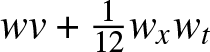 $w v+\frac{1}{12}w_x w_t$ is the momentum density, and
 $\phi(w)-w f(w)-\frac{1}{24}w_t^2-\frac{1}{2}v^2-\frac{1}{12}w w_{tt}$ is the momentum flux.
2.3. Averaged conservation laws
As shown in Section 3, under certain conditions, there exists a four-parameter family of periodic travelling wave solutions
 \begin{align}
w = w(\theta;\mathbf{r}), \quad v = v(\theta;\mathbf{r}),
\end{align}
of (2.7) with modulated phase
 \begin{align*}
\theta = S(X,T)/\epsilon, \quad \theta_x = S_X = k(X,T), \quad
\theta_t = S_T = -\omega(X,T),
\end{align*}
and parameters  $\mathbf{r} = (r_1,r_2,r_3,r_4)$ that are allowed to vary on slow spatio-temporal scales
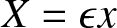 $X = \epsilon x$,
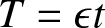 $T = \epsilon t$,
 $0 \lt \epsilon \ll 1$:
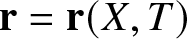 $\mathbf{r} = \mathbf{r}(X,T)$. The nonlinear dispersion relation yields
 $k(X,T) = k(\mathbf{r}(X,T))$,
 $\omega(X,T) = \omega(\mathbf{r}(X,T))$. We can formally obtain the Whitham modulation equations by averaging three conservation laws (2.7), (2.8) over a
 $2\pi$ period according to
 \begin{align}
\overline{w}_T - \overline{v}_X = 0,
\end{align}
 \begin{align}
\overline{v}_T - \overline{f(w)}_X = 0,
\end{align}
 \begin{align}
\left ( \overline{\phi(w)} + \frac{1}{2}\overline{v^2} +
\frac{\omega^2}{24} \overline{w_\theta^2} \right )_T - \left (
\overline{v f(w)} - \frac{\omega^2}{12}\overline{w_\theta v_\theta}
\right )_X = 0 ,
\end{align}
accompanied by the conservation of waves
 \begin{align}
S_{XT} = S_{TX} \quad \iff \quad k_T + \omega_X = 0 .
\end{align}
An additional conservation law, derivable from the previous set, is the average of momentum (2.9)
 \begin{align*}
\left(\overline{wv}-\dfrac{1}{12}k\omega \overline{w_\theta^2}
\right)_T-\left(\overline{w f(w)}+ \dfrac{1}{2}
\overline{v^2}- \overline{\phi(w)} - \dfrac{1}{24}
\omega^2\overline{w_\theta^2} \right)_X =0.
\end{align*}
 $2\pi$-periodic function
 $F(\theta)$ is defined according to
 \begin{align*}
\overline{F} \equiv \frac{1}{2\pi} \int_0^{2\pi}
F(\theta)\,\mathrm{d}\theta .
\end{align*}
3. Travelling wave solutions
We seek travelling wave solutions of eq. (2.1) in the form
 \begin{align}
u(x,t)=U(\xi), \quad \xi=x-ct,
\end{align}
where  $c$ is the velocity, and
 $\xi$ is the travelling wave coordinate. Substituting (3.1) into (2.1) and integrating, we obtain
 \begin{align}
c^2\left(w-\dfrac{1}{12}w''\right)=f(w)-\dfrac{A}{2},
\end{align}
where  $w=u_x=U'(\xi)$ is the strain, and
 $A$ is a constant of integration. Multiplying (3.2) by
 $w'(\xi)$ and integrating, we obtain
 \begin{align}
(w')^2=\dfrac{12}{c^2}(-2\phi(w)+c^2w^2+Aw+B),
\end{align}
where  $B$ is another integration constant. Equation (2.3) corresponds to
 \begin{align*}
\phi(w)=\dfrac{1}{2}w^2+\dfrac{\alpha}{3}w^3+\dfrac{\beta}{4}w^4,
\end{align*}
which together with (3.3) implies that
 \begin{align}
\begin{split}
(w')^2&= \dfrac{12}{c^2} \left( -\dfrac{\beta}{2} w^4-
\dfrac{2\alpha}{3} w^3+ (c^2-1) w^2+ Aw+ B \right)
\end{split}
\end{align}
must hold along periodic orbits. If  $\beta \neq 0$, we have
 \begin{align}
(w')^2=-\dfrac{6\beta}{c^2}G_4(w), \quad
G_4(w)=(w-w_1)(w-w_2)(w-w_3)(w-w_4),
\end{align}
where  $w_i$,
 $i=1,\dots,4$, are the four roots of the quartic polynomial
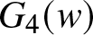 $G_4(w)$, numbered in increasing order of their real parts:
 $\text{Re} \ w_1 \leq \text{Re} \ w_2 \leq \text{Re} \ w_3 \leq
\text{Re} \ w_4$, followed by increasing order in the imaginary parts. It will be helpful to note the polynomial coefficients of
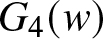 $G_4(w)$:
 \begin{align}
G_4(w) = w^4 + \frac{4\alpha}{3\beta} w^3 - \frac{2}{\beta}(c^2-1)
w^2 - \frac{2}{\beta} A w - \frac{2}{\beta} B .
\end{align}
In what follows, we will assume that at least two adjacent roots are real, which implies that either all four roots are real, or two are real and the other two are complex conjugates. Phase-plane analysis shows that this assumption is necessary for the existence of real-valued periodic orbits described by (3.5).
We can solve for a constraint on the roots and express  $c$ in terms of the roots by equating the coefficients of
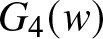 $G_4(w)$ in (3.5) and (3.6) to obtain
 \begin{align}
-\frac{4\alpha}{3\beta} = w_1 + w_2 + w_3 + w_4 ,
\end{align}
 \begin{align}
c^2 = 1 - \frac{\beta}{2} ( w_1 w_2 + w_1 w_3 + w_1 w_4 + w_2 w_3 +
w_2 w_4 + w_3 w_4 ).
\end{align}
Consequently, this is a three-parameter family of travelling wave solutions characterized by, for example, three of the roots. Both signs of  $c$ are possible but the root ordering must be maintained, which when
 $w_3$ and
 $w_4$ are real leads to the constraint
 \begin{align}
w_4 = -\frac{4\alpha}{3\beta} - w_1 - w_2 - w_3 \ge w_3 \quad \iff
\quad w_3 \le - \frac{2\alpha}{3\beta} - \frac{w_1+w_2}{2} .
\end{align}
Furthermore, the velocity  $c$ in (3.8) must be real, so we also require
 \begin{align}
1 \ge \frac{\beta}{2} ( w_1 w_2 + w_1 w_3 + w_1 w_4 + w_2 w_3 +
w_2 w_4 + w_3 w_4 ) .
\end{align}
Equating the two representations (3.5) and (3.6) of 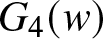 $G_4(w)$ also yields expressions for the integration constants in terms of the roots
 \begin{equation}
A = \frac{\beta}{2}(w_1w_2w_3 + w_1 w_2 w_4+w_1 w_3 w_4+w_2 w_3
w_4),
\end{equation}
 \begin{align}
B = -\frac{\beta}{2}w_1w_2w_3w_4 .
\end{align}
If  $\beta=0$ (
 $\alpha$-FPU interaction potential), there are only three roots, all required to be real and numbered in increasing order. In this case, (3.4) reduces to
 \begin{align}
(w')^2 =-\dfrac{8\alpha}{c^2}G_3(w), \quad G_3(w)=(w-w_1)(w-w_2)(w-w_3),
\end{align}
The expanded polynomial of 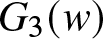 $G_3(w)$ from eq. (3.4) is
 \begin{equation}
G_3(w) = w^3 - \frac{3}{2\alpha}(c^2-1) w^2 - \frac{3}{2\alpha} A w
- \frac{3}{2\alpha} B .
\end{equation}
Equating the coefficients of 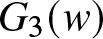 $G_3(w)$ in (3.13) and (3.14) determines the velocity-root relation
 \begin{equation}
c^2 = 1 + \frac{2\alpha}{3}(w_1+w_2+w_3),
\end{equation}
which requires  $\frac{2\alpha}{3}(w_1+w_2+w_3) \gt -1$ for real
 $c$. Thus, we again obtain a three-parameter family of travelling wave solutions. The coefficient relations of
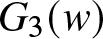 $G_3(w)$ also determine
 \begin{equation}
A = -\frac{2\alpha}{3}(w_1w_2+w_1w_3+w_2w_3),
\end{equation}
 \begin{equation}
B = \frac{2\alpha}{3}w_1w_2w_3 .
\end{equation}
Once  $\alpha$ and
 $\beta$ are fixed, the three-parameter family of travelling waves is parameterized by
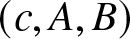 $(c,A,B)$ or, equivalently, by
 $(w_1,w_2,w_3)$. Below, we will identify an additional, physical parameterization
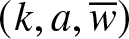 $(k,a,\overline{w})$ corresponding to the periodic travelling wave’s wavenumber
 $k$, amplitude
 $a$ and mean
 $\overline{w}$.
Although we will obtain three-parameter families of periodic travelling wave solutions for strain  $w$, the regularized Boussinesq equation also requires the determination of particle velocity
 $v$ in (2.7), which will introduce another integration constant. To fix this, we insert the travelling wave ansatz into the first equation in (2.7) and integrate to obtain
 \begin{equation}
v(\xi) = -c w(\xi) + V,
\end{equation}
where  $V$ is the integration constant. Averaging the latter expression over the period
 $L$ of the travelling wave in terms of
 $\xi$, we obtain
 $V$ as a mean accelerated particle velocity
 \begin{equation*}
V = \overline{v} + c \overline{w} = \frac{1}{L}\int_0^L (v(\xi) + c
w(\xi))\,\mathrm{d}\xi .
\end{equation*}
The periodic travelling wave solution (2.10) satisfying (3.4) can be parameterized by the roots  $w_1$,
 $w_2$,
 $w_3$ and the mean particle velocity
 $\overline{v}$. Collecting these into the vector
 \begin{equation}
\mathbf{W} = (w_1,w_2,w_3,\overline{v})^T,
\end{equation}
we will later consider alternative mathematically and physically convenient parameterizations.
We start by considering the general cubic nonlinearity (2.3) with  $\beta \neq 0$ and the orbit described by (3.5). First, we observe that in this case (3.2) becomes
 \begin{equation} w''=12\left((c^2-1)w-\alpha w^2-\beta
w^3+\dfrac{A}{2}\right).
\end{equation}
In what follows, we assume that the right-hand side of this equation has three real roots, corresponding to equilibrium points  $(w,w')=(w_*,0)$ in the phase plane. These equilibria are centres if
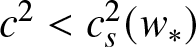 $c^2 \lt c_s^2(w_*)$ and saddles if
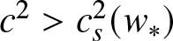 $c^2 \gt c_s^2(w_*)$. Depending on
 $\alpha$ and
 $\beta$, the phase plane of (3.20) for given
 $c$ and
 $A$ has either two centres separated by a saddle point (Fig. 1(a)) or two saddle points with a centre in between (Fig. 1(b)). Hence, the number of homoclinic orbits that enclose families of periodic trajectories is either two or one, respectively. Below, we consider these two cases separately.
(a) Periodic orbits for different values of  $B$ at
 $\alpha=0$,
 $\beta=1$,
 $c=3$,
 $A=-127/32$. The orbits on the left of the saddle point correspond to solutions (3.21) with
 $m=0.442$,
 $n=0.889$,
 $a=3.677$ (red),
 $m=0.216$,
 $n=0.694$,
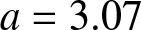 $a=3.07$ (green),
 $m=0$,
 $n=0.581$,
 $a=2.427$ (magenta),
 $n=0.255-0.049i$,
 $a=1.342$ (black). The orbits on the right correspond to the second family of solutions obtained via (3.33), with the same roots
 $w_i$ as the orbits of the same colour on the left but amplitude
 $a=w_4-w_3$ given by
 $a=2.595$ (red) and
 $a=1.779$ (green). (b) Periodic orbits at
 $\alpha=0$,
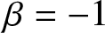 $\beta=-1$,
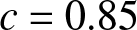 $c=0.85$,
 $A=11/400$ corresponding to (3.41) with
 $m=0.902$,
 $n=0.557$,
 $a=0.638$ (red),
 $m=0.769$,
 $n=0.445$,
 $a=0.474$ (green),
 $m=0.565$,
 $n=0.297$,
 $a=0.291$ (magenta),
 $m=0.239$,
 $n=0.111$,
 $a=0.099$ (black). (c) Periodic orbits at
 $\alpha=0$,
 $\beta=-1$,
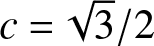 $c=\sqrt{3}/2$,
 $A=0$ corresponding to (3.41) with
 $m=0.924$,
 $n=0.726$,
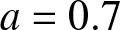 $a=0.7$ (red),
 $m=0.796$,
 $n=0.549$,
 $a=0.5$ (green),
 $m=0.4375$,
 $n=0.25$,
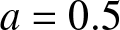
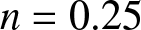
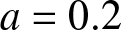 $a=0.2$ (magenta). (d) Solutions (3.41) (red) and its symmetric counterpart (blue) in the case (c) near the kink limit
 $m=n=a=1$. In panels (a–c), manifolds associated with the saddle points (including homoclinic and heteroclinic orbits) are shown in cyan.

1 Long description
The image A showing a phase plane plot with horizontal axis label w and vertical axis label w prime. The horizontal axis shows tick labels negative 4, negative 2, 2. The vertical axis shows tick labels 5 and negative 5. Four closed loops are drawn around a left-side center near w equals negative 3 and around a right-side center near w equals 3. The loops meet at a point at the origin where the two lobes touch. The image B showing a phase plane plot with horizontal axis label w and vertical axis label w prime. The horizontal axis shows tick labels negative 0.6, negative 0.4, negative 0.2, 0.2, 0.4, 0.6. The vertical axis shows tick labels 0.6, 0.4, 0.2, negative 0.2, negative 0.4, negative 0.6. Four nested closed loops are centered near the origin. Two open curves cross the horizontal axis near w equals negative 0.5 and w equals 0.5 and extend outward. The image C showing a phase plane plot with horizontal axis label w and vertical axis label w prime. The horizontal axis shows tick labels negative 0.6, negative 0.4, negative 0.2, 0.2, 0.4, 0.6. The vertical axis shows tick labels 0.6, 0.4, 0.2, negative 0.2, negative 0.4, negative 0.6. Three nested closed loops are centered near the origin. Two open curves cross the horizontal axis near w equals negative 0.5 and w equals 0.5 and extend outward. The image D showing a line graph with horizontal axis label theta and vertical axis label w. The horizontal axis shows tick labels 2, 4, 6, 8, 10, 12. The vertical axis shows tick labels 0.4, 0.2, negative 0.2, negative 0.4. Two curves alternate between a high plateau near w equals 0.5 and a low plateau near w equals negative 0.5, with steep transitions near theta values around 2, 5, 8 and 11.
3.1. Case I:  $\beta \gt 0$, two centres

As illustrated in Fig. 1(a), in this case there are two centres separated by a saddle point and thus two families of periodic orbits described by (3.5), with  $w_1 \leq w \leq w_2$ (below the saddle point) and
 $w_3 \leq w \leq w_4$ (above it), respectively. The first family of orbits is enclosed by the homoclinic trajectory corresponding to a compressive (depression or dark) solitary wave, and the second by a homoclinic orbit corresponding to a tensile (elevation or bright) solitary wave.
To obtain the first family, we need to solve (3.5) for  $w(\xi)$ in the interval
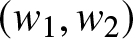 $(w_1,w_2)$, where
 $w_1$ and
 $w_2$ must be real and distinct. Using separation of variables and an appropriate substitution to evaluate the integral involving
 $w$ [Reference Byrd and Friedman4], we obtain
 \begin{equation}
\begin{split}
w(\theta) &= \frac{w_1+w_4n\, \mathrm{sn}^2\left (
\frac{K(m)}{\pi} \theta; m \right )}{1 +n\,\mathrm{sn}^2\left (
\frac{K(m)}{\pi} \theta; m \right )}, \quad
m = \frac{(w_4-w_3)(w_2-w_1)}{(w_4-w_2)(w_3-w_1)}, \quad n=\dfrac{w_2-w_1}{w_4-w_2},
\end{split}
\end{equation}
where  $\text{sn}$ is the Jacobi elliptic sine function and
 $K(m)$ is the complete elliptic integral of the first kind. The solution (3.21) is
 $2\pi$-periodic,
 $w(\theta + 2\pi) = w(\theta)$, in the phase
 $\theta = k\xi = kx - \omega t$ with wavenumber
 $k$ and nonlinear frequency
 $\omega$ given by
 \begin{equation}
k = \frac{\pi}{K(m)} \sqrt{\frac{3\beta}{2c^2}(w_4-w_2)(w_3-w_1)}, \quad \omega=ck,
\end{equation}
where we recall (3.8), the wavelength 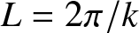 $L = 2\pi/k$, and the temporal period
 $T = 2\pi/\omega$. The physical parametrization of this solution is
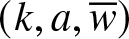 $(k,a,\overline{w})$, where the wavenumber
 $k$ in (3.22), the amplitude
 $a = w_2 - w_1$ and the mean
 \begin{equation}
\overline{w}=\frac{1}{2\pi}\int_0^{2\pi} w(\theta)\,\mathrm{d}\theta = w_4-\dfrac{\Pi(-n,m)}{K(m)}(w_4-w_1)
\end{equation}
are all determined in terms of the roots  $w_1$,
 $w_2$,
 $w_3$ in view of (3.7). The function
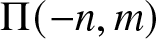 $\Pi(-n,m)$ is the complete elliptic integral of the third kind with
 $n$ given in (3.21).
Note that the solution (3.21) only requires  $w_1$ and
 $w_2$ to be real and also works in the case when
 $w_3$ and
 $w_4$ are non-real complex conjugates. In this case,
 $m$ and
 $n$ are complex but the solution itself and
 $k$,
 $a$,
 $\overline{w}$ are real. An example of a periodic orbit with complex
 $w_{3,4}$ is the black trajectory in Fig. 1(a). In the case when
 $w_3$ and
 $w_4$ are real, the root ordering
 $w_1 \lt w_2 \lt w_3 \lt w_4$ implies that
 \begin{equation}
n \gt 0, \quad 0 \lt m \lt 1.
\end{equation}
If these roots are complex conjugates,  $w_{3,4}=\rho \mp i\eta$,
 $\eta \gt 0$, (3.7) implies that
 $\rho=-(4\alpha/(3\beta)+w_1+w_2)/2$, and the ordering
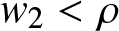 $w_2 \lt \rho$ thus means that
 $4\alpha + 3\beta (w_1 + 3 w_2) \lt 0$, which together with
 $w_1 \lt w_2$ yields
 \begin{equation}
\begin{split}
&\text{Re}(n)=-\dfrac{6\beta (w_2 - w_1) (4\alpha + 3\beta (w_1 + 3 w_2))}{36 \beta^2 \eta^2 + (4 \alpha + 3\beta (w_1 + 3 w_2))^2} \gt 0, \\
&\text{Im}(n)=-\dfrac{36 \beta^2 \eta (w_2 - w_1)}{36\beta^2 \eta^2 + (4\alpha + 3\beta (w_1 + 3 w_2))^2} \lt 0.
\end{split}
\end{equation}
As we will show below, in this case, we can obtain  $m$ in terms of real and imaginary parts of
 $n$.
The bifurcation from real to complex conjugate roots occurs in the limit  $w_3 \to w_4$ where
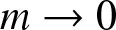 $m \to 0$ so that the solution (3.21) is the trigonometric wave
 \begin{equation}
w(\theta) = \frac{w_1 + w_4 n \sin^2(\theta/2)}{1 + n
\sin^2(\theta/2)},
\end{equation}
whose wavenumber, amplitude and mean are
 \begin{equation}
k = 2 \sqrt{\frac{3\beta}{2c^2}(w_4-w_2)(w_4-w_1)}, \quad a = w_2
- w_1, \quad \overline{w} = w_4 - \frac{w_4-w_1}{\sqrt{1+n}} .
\end{equation}
Since  $2w_4 = -4 \alpha/(3\beta) - w_1 - w_2$ by virtue of (3.7), the trigonometric wave (3.26) is a two-parameter family of solutions. An example orbit given by the trigonometric solution (3.26) is the magenta trajectory in Fig. 1(a).
In the limit  $w_2 \to w_1$ in eq. (3.21),
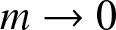 $m \to 0$, and the solution exhibits the following asymptotic behaviour:
 \begin{equation*}
w(\theta) = w_1 - \frac{1}{2}(w_2 -w_1)\cos\theta + \dots ,
\quad \theta = kx - \omega_0 t,
\end{equation*}
where, upon utilizing (3.7), (3.8), (3.22) and (3.23), we obtain the linear dispersion relation (2.4) for small-amplitude (linear) waves propagating on the constant background 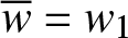 $\overline{w} = w_1$.
In the limit  $w_2 \to w_3$,
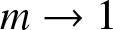 $m \to 1$, and the solution (3.21) approaches the depression solitary wave
 \begin{equation}
w(\xi) = \frac{w_1 + w_4 n\,
\mathrm{tanh}^2(\xi/\ell)}{1 + n\,
\mathrm{tanh}^2(\xi/\ell)} , \quad n = \frac{w_3-w_1}{w_4-w_3},
\quad \ell = \left (\frac{3\beta}{2c^2}(w_4-w_3)(w_3-w_1) \right
)^{-1/2},
\end{equation}
with amplitude  $a = w_3-w_1$ propagating on the background
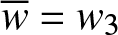 $\overline{w} = w_3$. An example of the corresponding trajectory is shown by the left cyan loop in Fig. 1(a). These depression solitary waves form a two-parameter family of solutions with velocity-amplitude relation
 \begin{equation}
c^2 = c_s^2(\overline{w}) + \frac{1}{2} a^2 \beta-\frac{2}{3} a(\alpha + 3 \beta\overline{w}) .
\end{equation}
Strict inequality 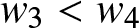 $w_3 \lt w_4$ and (3.7) imply that these waves exist when
 \begin{equation}
\overline{w} \lt -\dfrac{\alpha}{3\beta},~ a \gt 0 \quad \text{or} \quad a \gt 4\left(\overline{w}+\dfrac{\alpha}{3\beta}\right) \gt 0,
\end{equation}
which means that 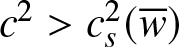 $c^2 \gt c_s^2(\overline{w})$ in (3.29), and thus the waves are supersonic. Note that this implies that for
 $\overline{w} \gt -\alpha/(3\beta)$ the amplitude has a strictly positive lower bound.
In the limit  $w_2 \to w_3 \to w_4$, we have
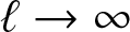 $\ell \to \infty$, so that
 $\tanh^2(\xi/\ell) \sim (\xi/\ell)^2$ in eq. (3.28), and the algebraically decaying depression solitary wave is obtained,
 \begin{equation}
w(\xi) = \frac{2 w_1 - 3 \beta w_4 \left ( w_1(w_4+w_1) -
(w_4-w_1)^2 \xi^2 \right )}{2 - 3 \beta \left ( w_4(w_4+w_1) -
(w_4-w_1)^2 \xi^2 \right )},
\end{equation}
with amplitude  $a = w_4 - w_1$ and background
 $\overline{w} = w_4$. By virtue of (3.7), this is a one-parameter family of algebraic solitary waves subject to the amplitude-background constraint
 $a = 4(\overline{w} + \alpha/(3\beta)) \gt 0$. These waves propagate with sound velocity,
 \begin{equation}
c^2 = 1 + 3\beta\overline{w}(\tfrac{1}{2} a - \overline{w})=c_s^2(\overline{w}),
\end{equation}
and thus represent the nontrivial sonic limit of (3.28) [Reference Vainchtein37]. The algebraic solitary wave solution (3.31) can alternatively be obtained by taking the limit  $w_2 \to w_4$ in the trigonometric wave (3.26) because in this limit
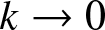 $k \to 0$ while
 $n \to \infty$, so that
 $n \sin^2(k\xi) \sim n (k\xi)^2 \to 6\beta(w_4-w_1)^2\xi^2/c^2$.
The second periodic travelling wave family (illustrated by the right set of orbits in Fig. 1(a)) solves (3.5) in 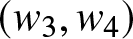 $(w_3,w_4)$ with real and distinct
 $w_3$ and
 $w_4$. It is readily obtained from the first family by using the symmetry of the problem, which amounts to making the following replacements in (3.21):
 \begin{equation}
\begin{split}
&w(\theta) \to -w(\theta)-\dfrac{2\alpha}{3\beta},\\
&w_1 \to -w_4-\dfrac{2\alpha}{3\beta}, \quad w_2 \to -w_3-\dfrac{2\alpha}{3\beta},
\quad w_3 \to -w_2-\dfrac{2\alpha}{3\beta},
\end{split}
\end{equation}
where the roots are renumbered to keep their nondecreasing order. The solution has the amplitude  $a = w_4 - w_3$ and the same wavenumber (3.22), wavelength, frequency and period as the solutions (3.21). It leads to a two-parameter family of trigonometric solutions in the limit
 $w_2 \to w_1$, a two-parameter elevation solitary wave family in the limit
 $w_3 \to w_2$, and a one-parameter family of sonic algebraic elevation waves when
 $w_3 \to w_2 \to w_1$.
For simplicity, we now consider  $(\alpha,\beta)=(0,1)$, recalling that one can always reduce the case
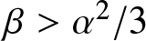 $\beta \gt \alpha^2/3$ to these parameter values upon a proper rescaling, as discussed in Section 2.1. The periodic travelling wave solution (3.21) can be parameterized by
 $\mathbf{W}$ in (3.19), which involves the first three roots and the mean particle velocity. First, we consider the case when all four roots are real. In this case, (3.7) and (3.8) for
 $\alpha=0$ and
 $\beta=1$ imply
 \begin{equation*}
c^2=1+\dfrac{1}{4}\left((w_1+w_2)^2+(w_2+w_3)^2+(w_1+w_3)^2\right) \geq 1,
\end{equation*}
so that  $c$ is always real (eq. (3.10) holds), and we have
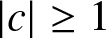 $|c|\geq 1$. A second, useful parameterization involves the elliptic function parameters
 $n$,
 $m$, and the wave amplitude
 $a$:
 \begin{equation}
\mathbf{A} = (n,m,a,\overline{v})^T.
\end{equation}
The transformation 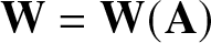 $\mathbf{W} = \mathbf{W}(\mathbf{A})$ and its Jacobian determinant are
 \begin{equation}
\begin{split}
w_1 &= a \Xi(n,m)\gamma_1(n,m), \quad
w_2 = a \Xi(n,m) \gamma_2(n,m), \quad
w_3 = a \Xi(n,m) \gamma_3(n,m), \\
\Xi &=\frac{1}{4n(m+n)} , \quad
\det \left (\frac{\partial \mathbf{W}}{\partial \mathbf{A}}
\right )
= \frac{a^2(1+n)}{4n^2(m+n)^2} ,
\end{split}
\end{equation}
where
 \begin{equation*}
\begin{split}
\gamma_1 &= -3n^2 - 2(1+m)n - m, \quad
\gamma_2 = n^2 - 2n(1-m) - m, \\
\gamma_3 &= n^2 + 2n(1-m) - m .
\end{split}
\end{equation*}
For  $a \gt 0$ and (3.24), the transformation (3.35) is invertible. In these variables, the existence of periodic travelling waves is restricted by (3.24):
 \begin{equation}
\mathbf{A} \in E_a = \left \{ (n,m,a,\overline{v})^T \in \mathbb{R}^4 \,|\, n \gt 0, ~0 \lt m \lt 1,~a \gt 0 \right \}.
\end{equation}
Another parameterization results by transforming  $a$ in
 $\mathbf{A}$ to the wave frequency
 \begin{equation}
\omega = \mathrm{sgn}(c)\frac{\pi a}{K(m)}
\sqrt{\frac{3(1+n)}{2n(m+n)}} ,
\end{equation}
which is invertible when (3.36) holds. Similar transformations to  $k$ and
 $\overline{w}$ can also be obtained.
For the case of complex conjugate roots  $w_{3,4}=-\frac{1}{2}(w_1+w_2) \mp i\eta$,
 $\eta \gt 0$, it is convenient to use
 \begin{equation}
\mathbf{\tilde{A}}=(n_r,n_i,a,\overline{v})^T
\end{equation}
as the parametrisation, where  $n_r=\text{Re}(n) \gt 0$ and
 $n_i=\text{Im}(n) \lt 0$ by (3.25). This yields the transformation
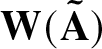 $\mathbf{W}(\mathbf{\tilde{A}})$
 \begin{equation}
\begin{split}
w_1=-\dfrac{a}{4}\left(3 + \dfrac{2 n_r}{n_i^2 + n_r^2}\right), \quad
&w_2=\dfrac{a}{4}\left(1 - \dfrac{2 n_r}{n_i^2 + n_r^2}\right), \quad
w_3=\dfrac{a}{4}\left(1 + \dfrac{2 n_r}{n_i^2 + n_r^2}\right)+i\dfrac{a n_i}{n_i^2 + n_r^2}, \\
&\det \left (\frac{\partial \mathbf{W}}{\partial \mathbf{\tilde{A}}}
\right )
= \frac{i a^2}{2(n_i^2 + n_r^2)^2},
\end{split}
\end{equation}
that is invertible for  $a \gt 0$ with
 \begin{equation*}
m=\dfrac{2 n_i}{n_i + i(1 + n_r)}.
\end{equation*}
Recalling (3.25) and (3.10), we observe that periodic travelling waves exist when
 \begin{equation}
\begin{split}
&\mathbf{\tilde{A}} \in \tilde{E}_a = \bigg\{ (n_r,n_i,a,\overline{v})^T
\in \mathbb{R}^4\,|\, n_r \gt 0, ~n_i \lt 0,~a \gt 0,\\
&\qquad\qquad\qquad 16 + a^2 \left(3 + \dfrac{4 (n_i^2 (n_r - 2) +
n_r^2 (1 + n_r))}{(n_i^2 + n_r^2)^2}\right) \gt 0 \bigg\}.
\end{split}
\end{equation}
The transition from real roots to a pair of complex conjugate roots occurs when  $w_3 \to w_4$, so that
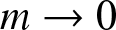 $m \to 0$. Passing to this limit in (3.35), (3.37) and (3.27) for
 $(\alpha,\beta) = (0,1)$, we can eliminate
 $n$ and identify the crossover dispersion relation
 \begin{equation*}
\omega^2 = k^2 \frac{48 + 9a^2}{48-2k^2}, \quad 0 \le k \lt 2 \sqrt{6} ,
\end{equation*}
holding for the trigonometric solution (3.26) with wave speed satisfying  $c^2 = 1 + \frac{3}{16} a^2 + \frac{1}{24} \omega^2$.
3.2. Case II, β < 0, single centre
In this case, as shown in Fig. 1(b), there are two saddle points separated by a centre, and hence periodic orbits satisfy (3.5) in 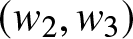 $(w_2,w_3)$, where
 $w_2$ and
 $w_3$ are real and distinct. One family of periodic travelling waves is given by [Reference Chong, Herrmann and Kevrekidis6]
 \begin{equation}
w(\theta)=\dfrac{w_2-w_1n\,\text{sn}^2\left
(\frac{K(m)}{\pi}\theta;m \right )}
{1-n\, \text{sn}^2 \left (\frac{K(m)}{\pi} \theta;m \right )},
\quad m=\dfrac{(w_4-w_1)(w_3-w_2)}{(w_4-w_2)(w_3-w_1)} , \quad
n = \frac{w_3-w_2}{w_3-w_1},
\end{equation}
where root ordering  $w_1 \lt w_2 \lt w_3 \lt w_4$ implies
 \begin{equation}
0 \lt n \lt m \lt 1 .
\end{equation}
The physical parameters 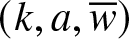 $(k,a,\overline{w})$ are the wavenumber
 \begin{equation}
k = \frac{\pi}{K(m)}\sqrt{\frac{3|\beta|}{2 c^2}(w_4-w_2)(w_3-w_1)},
\end{equation}
the non-negative amplitude  $a = w_3 - w_2$, and the mean strain
 \begin{equation}
\overline{w} = w_1+\dfrac{\Pi(n,m)}{K(m)}(w_2-w_1).
\end{equation}
Examples of orbits computed using (3.41) are shown in Figure 1(b).
In the limit  $w_3 \to w_2$,
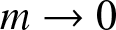 $m \to 0$, and
 \begin{equation*}
w(\theta) = w_2 - \frac{1}{2}(w_3-w_2)\cos(\theta) + \dots, \quad
\theta = kx - \omega_0t,
\end{equation*}
subject to the linear dispersion relation (2.4) with 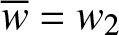 $\overline{w} = w_2$.
When  $w_3 \to w_4$,
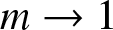 $m \to 1$ and we obtain a two-parameter family of depression solitary waves [Reference Vainchtein and Truskinovsky36]
 \begin{equation}
w(\xi) = \frac{w_2 - w_1 n\,
\mathrm{tanh}^2(\xi/\ell)}{1 - n\,
\mathrm{tanh}^2(\xi/\ell)} , \quad n = \frac{w_4-w_2}{w_4-w_1},
\quad \ell =
\left ( \frac{3|\beta|}{2c^2}(w_4-w_2)(w_4-w_1) \right )^{-1/2} ,
\end{equation}
with amplitude  $a = w_4 - w_2$, propagating on the background
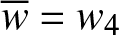 $\overline{w} = w_4$ with velocity-amplitude relation
 \begin{equation}
c^2 = c_s^2(\overline{w}) + \frac{1}{2} \beta a^2 -
\frac{2}{3}a(\alpha+3\beta\overline{w}).
\end{equation}
An example of the corresponding homoclinic trajectory is shown by the cyan loop in Fig. 1(b). Using root ordering  $w_1 \lt w_2 \lt w_4$, (3.7) and requiring that
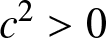 $c^2 \gt 0$ in (3.46), we obtain the existence conditions
 \begin{equation}
0 \lt a \lt 2 \left ( \overline{w} + \frac{\alpha}{3 \beta} \right ) , \quad \overline{w} +
\frac{\alpha}{3\beta} \gt 0, \quad c_s^2(\overline{w}) + \frac{1}{2} \beta a^2 -
\frac{2}{3}a(\alpha+3\beta\overline{w}) \gt 0.
\end{equation}
Note that these conditions impose an upper bound on the amplitude of the solitary wave, as well as upper and lower bounds on  $\overline{w}$, in contrast to the waves (3.28), whose amplitude can be arbitrarily large for any
 $\overline{w}$ but may have a strictly positive lower bound (recall (3.30)). We also remark that the first two conditions in (3.47) imply that the solitary waves are supersonic, i.e.,
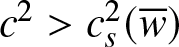 $c^2 \gt c_s^2(\overline{w})$ in (3.46), and thus the third inequality is automatically satisfied when
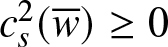 $c_s^2(\overline{w}) \geq 0$. However, this inequality must be imposed when
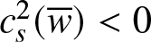 $c_s^2(\overline{w}) \lt 0$ to ensure that
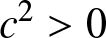 $c^2 \gt 0$.
Another family of periodic travelling waves is related to the first family via the symmetry transformation (3.33). One can show that the two families differ by a  $\pi$ shift in phase
 $\theta$ and have the same mean, wave number and amplitude. In the limit
 $w_2 \to w_1$, the second family of periodic orbits approaches the two-parameter family of elevation solitary waves that can be obtained from (3.45) using (3.33).
The case in which  $w_2 \to w_1$ and
 $w_3 \to w_4$ results in heteroclinic orbits described by supersonic kink solutions that are given by [Reference Vainchtein and Truskinovsky36]
 \begin{equation}
w(\xi)=\dfrac{w_1+w_4}{2} \pm \dfrac{w_4-w_1}{2}\tanh(\xi/\ell), \quad \ell = \frac{2|c|}{\sqrt{6|\beta|}(w_4-w_1)},
\end{equation}
where
 \begin{equation}
w_1+w_4=-\dfrac{2\alpha}{3\beta}, \quad c^2=1-\dfrac{\alpha^2}{3\beta}+\beta\left(w_1+\dfrac{\alpha}{3\beta}\right)^2.
\end{equation}
This is a one-parameter family of kink and antikink solutions. If the plus sign is chosen in (3.48), 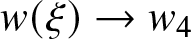 $w(\xi) \to w_4$ as
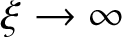 $\xi \to \infty$ and
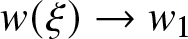 $w(\xi) \to w_1$ as
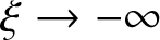 $\xi \to -\infty$ (an antikink). With the minus sign, we have
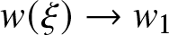 $w(\xi) \to w_1$ as
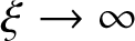 $\xi \to \infty$ and
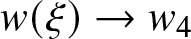 $w(\xi) \to w_4$ as
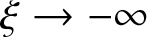 $\xi \to -\infty$ (a kink). The amplitude
 $a=w_4-w_1$ of the kink is the upper bound (3.47) of the solitary wave amplitude for solutions (3.45) and their symmetric counterparts. When
 $(\alpha,\beta) = (0,-1)$, we have
 $w_1=-w_4$,
 $c^2=1-w_1^2=1-w_4^2$ by (3.49), and the solution (3.48) simplifies to
 \begin{equation*}
w(\xi) = \pm w_4 \,\mathrm{tanh} \left ( w_4 \sqrt{\frac{6}{1-w_4^2}} \ \xi \right ).
\end{equation*}
Examples of periodic orbits approaching the heteroclinic ones are shown in Fig. 1(c). The two families of periodic solutions yield the same trajectories. Near the heteroclinic orbits, the solution acquires the flat-top structure of a periodic kink-antikink lattice shown in Fig. 1(d).
In what follows, we consider the case  $(\alpha,\beta)=(0,-1)$ without loss of generality. The periodic travelling wave solution (3.41) can be parameterized by
 $\mathbf{W}$ in (3.19) subject to the existence inequalities (3.9) and (3.10). As before, we can also introduce the alternative parameterization
 $\mathbf{A}$ in (3.34) involving the amplitude
 $a$.
The transformation 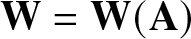 $\mathbf{W} = \mathbf{W}(\mathbf{A})$ and its Jacobian determinant are
 \begin{equation}
\begin{split}
w_1 &= a \Xi(n,m)\gamma_1(n,m), \quad
w_2 = a \Xi(n,m) \gamma_2(n,m), \quad
w_3 = a \Xi(n,m) \gamma_3(n,m), \\
\Xi &=\frac{1}{4n(m-n)} , \quad
\det \left (\frac{\partial \mathbf{W}}{\partial \mathbf{A}}
\right )
= \frac{a^2(1-n)}{4n^2(m-n)^2} ,
\end{split}
\end{equation}
where
 \begin{equation*}
\begin{split}
\gamma_1 &= -n^2 + 2(1+m)n - 3m, \quad \gamma_2 = 3n^2 -
2n(1+m) + m, \\
\gamma_3 &= -n^2 - 2n(1-m) + m .
\end{split}
\end{equation*}
When  $a \gt 0$ and (3.42) hold, the transformation (3.50) is invertible. Periodic travelling wave existence is subject to (3.42) and a real wave speed requiring (3.10):
 \begin{equation*}
\begin{split}
\mathbf{A} \in E_a &= \bigg \{ (n,m,a,\overline{v})^T \in \mathbb{R}^4
\,|\, 0 \lt n \lt m \lt 1, ~ 0 \lt a \lt a_{\rm max}(n,m)\bigg \}, \\
a_{\rm max} &= \frac{\sqrt{2}}{\Xi(n,m)P(n,m)},
\end{split}
\end{equation*}
where
 \begin{equation*}
\begin{split}
P(n,m) &= \sqrt{\gamma_1 \gamma_2
+ \gamma_1 \gamma_3 + \gamma_2 \gamma_3-(\gamma_1 +
\gamma_2 + \gamma_3)^2} \\
&= \sqrt{6 n^4 - 8(1+m)n^3 + 4(2+m+2m^2)n^2 -8 m(1+m)n + 6m^2}.
\end{split}
\end{equation*}
The amplitude upper bound 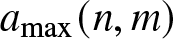 $a_{\rm max}(n,m)$ is an increasing function of its arguments with
 $a_{\rm max}(0,0) = a_{\rm max}(0,m) = \lim_{n\to m}a_{\rm max}(n,m) =
0$ for
 $0 \lt m \lt 1$ and
 $\lim_{n \to 1}\lim_{m\to 1} a_{\rm max}(n,m) = 2$ so that all periodic travelling waves are constrained to have amplitudes in the interval
 $0 \lt a \lt 2$.
We can obtain other parameterizations by, for example, transforming  $a$ in
 $\mathbf{A}$ to the wave frequency
 \begin{equation*}
\omega = \mathrm{sgn}(c)\frac{\pi a}{K(m)}
\sqrt{\frac{3(1-n)}{2n(m-n)}} ,
\end{equation*}
which is invertible when (3.42) holds. Similar transformations to  $k$ and
 $\overline{w}$ can also be obtained.
3.3. Case III:
$\beta=0$, single family of periodic orbits

In this case, eq. (3.20) has a quadratic polynomial in the right-hand side, and we focus on the case of two real roots, corresponding to two equilibrium points 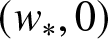 $(w_*,0)$ in the phase plane. If
 $\alpha \gt 0$, there is a saddle point on the left, and a centre on the right, so that the homoclinic trajectory enclosing the periodic orbits corresponds to a tensile (bright) solitary wave (see Figure 2). If
 $\alpha \lt 0$, the centre is on the left, and the saddle is on the right so that the homoclinic trajectory corresponds to a compressive (dark) solitary wave. Recall that, in this case, the periodic orbits satisfy (3.13). For
 $\alpha \gt 0$, we have
 $w_2 \leq w \leq w_3$, and the solution is given by [Reference Kamchatnov25]
 \begin{equation}
w(\theta)=w_3-(w_3-w_2)\text{sn}^2\left(\frac{K(m)}{\pi}\theta\right), \quad m=\dfrac{w_3-w_2}{w_3-w_1},
\end{equation}
Periodic orbits for different values of  $B$ at
 $\alpha=1$,
 $\beta=0$,
 $c=2.5$,
 $A=-8.5$ corresponding to (3.51) with
 $m=0.9225$,
 $a=4.6671$,
 $\overline{w}=2.8434$ (red),
 $m=0.66971$,
 $a=3.6995$,
 $\overline{w}=3.5976$ (green),
 $m=0.3994$,
 $a=2.2333$,
 $\overline{w}=4.0457$ (purple),
 $m=0.22765$,
 $a=1.2224$,
 $\overline{w}=4.1915$ (magenta). Manifolds associated with the saddle point (including the homoclinic orbit) are shown in cyan.

with amplitude  $a=w_3-w_2$, wavenumber
 \begin{equation}
k=\dfrac{\pi}{K(m)}\sqrt{\dfrac{2|\alpha|}{c^2}(w_3-w_1)}
\end{equation}
and mean
 \begin{equation}
\overline{w}=w_1+(w_3-w_1)\dfrac{E(m)}{K(m)},
\end{equation}
where  $E(m)$ is the complete elliptic integral of the second kind. Example trajectories are shown in Fig. 2.
The harmonic limit when  $w_3 \to w_2$, and thus
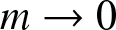 $m \to 0$, is described by
 \begin{equation*}
w(\theta) = w_2 + \frac{1}{2}(w_3-w_2)\cos(\theta) + \dots, \quad \theta = kx-\omega_0t,
\end{equation*}
with  $\omega_0$ corresponding to the linear dispersion relation (2.4) on the background
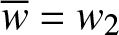 $\overline{w} = w_2$. In the limit
 $w_2 \to w_1$,
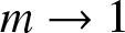 $m \to 1$, and we obtain the two-parameter family of elevation solitary waves
 \begin{equation*}
w(\xi)=w_3-(w_3-w_1)\text{tanh}^2(\xi/l), \quad l=\left(\dfrac{2\alpha}{c^2}(w_3-w_1)\right)^{-1/2},
\end{equation*}
with amplitude  $a=w_3-w_1$, propagating on the background
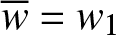 $\overline{w}=w_1$ with velocity-amplitude relation
 \begin{equation*}
c^2=c_s^2(\overline{w})+\dfrac{2\alpha}{3}a,
\end{equation*}
where we used (3.15). See the cyan loop in Fig. 2 for an example of the corresponding homoclinic orbit.
For  $\alpha \lt 0$, we have
 $w_1 \leq w \leq w_2$, and the solution can be obtained from (3.51) using the symmetry transformation
 \begin{equation*}
w(\theta) \to -w(\theta), \quad w_3 \to -w_1, \quad w_2 \to -w_2, \quad w_1 \to -w_3,
\end{equation*}
where again the roots are renumbered to keep their nondecreasing order. In the limit when  $w_2 \to w_3$, it yields a family of depression solitary waves.
In what follows, we assume  $\alpha = 1$. In addition to the parameterization
 $\mathbf{W}$ in (3.19) in terms of the roots, it is advantageous to introduce the parameterization
 \begin{equation}
\overline{\mathbf{A}} = (m,a,\overline{v},\overline{w})^T .
\end{equation}
The transformation 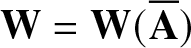 $\mathbf{W} = \mathbf{W}(\overline{\mathbf{A}})$ and its Jacobian determinant are
 \begin{equation*}
\begin{split}
w_1 &= \frac{m\overline{w} K(m) - aE(m)}{m K(m)}, \quad w_2 =
\frac{m K(m)(\overline{w}-a) - a(E(m)-K(m))}{mK(m)}, \\
w_3 &= \frac{m\overline{w} K(m) - a(E(m)-K(m))}{mK(m)} , \quad \det\left (
\frac{\partial \mathbf{W}}{\partial \overline{\mathbf{A}}}
\right ) = - \frac{a}{m^2} ,
\end{split}
\end{equation*}
demonstrating invertibility for  $a \gt 0$ and
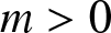 $m \gt 0$.
The positivity of the squared wave speed (3.15) implies that the mean strain (3.53) exhibits the lower bound
 \begin{equation}
\overline{w} \gt \overline{w}_{\rm min} = a \frac{3 E(m)-(2-m)K(m)}{3 m K(m)} - \frac{1}{2} .
\end{equation}
The minimum mean is a decreasing function of  $m$, exhibiting the limits
 $\lim_{m \to 1} \overline{w}_{\rm min} = -\frac{1}{2} - \frac{a}{3}$,
 $\lim_{m \to 0} \overline{w}_{\rm min} = -\frac{1}{2} + \frac{\omega_0^2}{24}$. Thus, the minimum mean satisfies
 \begin{equation}
-\frac{a}{3} \le \overline{w}_{\rm min} +\frac{1}{2} \le \frac{\omega_0^2}{24} .
\end{equation}
The periodic travelling wave existence criteria are
 \begin{equation}
\overline{\mathbf{A}} \in \overline{E}_a = \bigg \{(m,a,\overline{v},\overline{w})^T
\in \mathbb{R}^4 \, | \, 0 \le m \le 1, ~ a \gt 0, ~ \overline{w} \gt \overline{w}_{\rm min} \bigg \} .
\end{equation}
It first attains the value 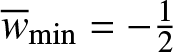 $\overline{w}_{\rm min} = -\frac{1}{2}$ when
 $m = m_* \approx 0.96115$ satisfying
 $3 E(m_*)-(2-m_*)K(m_*)$ = 0. That is, for
 $0 \lt m \lt m_*$, the periodic travelling wave existence criteria include
 $\overline{w} \gt \overline{w}_{\rm min}(m,a) \gt -\frac{1}{2}$. When
 $m_* \le m \le 1$,
 $\overline{w} \gt \overline{w}_{\rm min}(m,a) \ge -\frac{1}{2} - \frac{a}{3}$, i.e., the mean can fall below the value
 $-\frac{1}{2}$. It will be convenient for later analysis to express the admissible set
 $\overline{E}_a$ as the union of two (not disjoint) subsets
 \begin{equation}
\begin{split}
\overline{E}_a &= \overline{E}^{(a)}_a \cup \overline{E}^{(b)}_a ,
\\
\overline{E}^{(\rm a)}_a &= \bigg \{\overline{\mathbf{A}} \in
\mathbb{R}^4 \, | \, 0 \lt m \lt 1, ~ 0 \lt a \lt a_{\rm max}(m,\overline{w}), ~ \overline{w} \gt -\frac{1}{2}
\bigg \} , \\
\overline{E}^{(\rm b)}_a &= \bigg \{\overline{\mathbf{A}} \in
\mathbb{R}^4 \, | \, m_* \approx 0.96115 \lt m \lt 1, ~ 0 \lt a ,
~ \overline{w}_{\rm min}(m,a) \lt \overline{w}
\bigg \} .
\end{split}
\end{equation}
Here, the upper bound on the amplitude of the periodic travelling wave is
 \begin{equation}
a_{\rm max}(m,\overline{w}) =
\begin{cases}
3 \left ( \frac{1}{2} + \overline{w} \right ) \frac{m K(m)}{3
E(m) - (2-m)K(m)}, & 0 \lt m \lt m_* , \\
\infty, & m_* \lt m \lt 1 .
\end{cases}
\end{equation}
Since
 \begin{equation}
\omega = \mathrm{sgn}(c)\frac{\pi\sqrt{2a/m}}{K(m)},
\end{equation}
we can invertibly transform  $a \to \omega$ in (3.54) within the admissible region.
When  $a \to a_{\rm max}$ for
 $0 \lt m \lt m_*$, the periodic travelling wave velocity
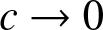 $c \to 0$ but the frequency
 $\omega$ remains finite so that the wavenumber
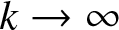 $k \to \infty$. Consequently, this is the short-wavelength limit.
4. Whitham modulation equations
The Whitham modulation equations are obtained from an ansatz consisting of a slowly varying periodic travelling wave [Reference Whitham39]. The modulation equations describe the projection of the PDE dynamics of (2.1) onto the manifold of periodic travelling waves constrained by a quasilinear system of first-order PDEs of hydrodynamic type [Reference Dubrovin and Novikov14].
There are several equivalent approaches to obtain the modulation equations. Perhaps the simplest is the average conservation law approach described in Section 2.3. Insertion of the appropriate periodic travelling wave family (one of eqs. (3.21), (3.41), (3.51)) into eq. (2.11) yields the Whitham modulation equations directly. One benefit of this approach is that the conservation form is obtained immediately. One drawback to this form of the modulation equations is that a direct computation of the solitary-wave limit is singular because 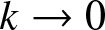 $k \to 0$ and one of the averaged conservation laws, e.g., (2.11c), is equivalent to (2.11a) and (2.11b) in this limit. Consequently, one equation for the modulations is not determined.
Another mathematically appealing approach to the derivation of the Whitham modulation equations is the method of multiple scales. A suitable ansatz and solvability conditions result in the modulation equations [Reference El and Hoefer16].
Yet another approach to obtain the Whitham modulation equations is the averaged variational principle [Reference Whitham39]. Integrating the Lagrangian  $\mathbb{L}(\theta)$ in eq. (2.6) over a period of the travelling wave family leads to the average Lagrangian
 $\mathcal{L}(\mathbf{r}) = \frac{1}{2\pi} \int_0^{2\pi}
\mathbb{L}(\theta)\,\mathrm{d}\theta$, where
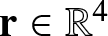 $\mathbf{r} \in \mathbb{R}^4$ are the periodic travelling wave’s parameters. The Euler-Lagrange equations for the averaged Lagrangian are the Whitham modulation equations. One benefit of this approach is that an additional conservation law, the conservation of wave action
 \begin{equation*}
\partial_T \mathcal{L}_\omega - \partial_X \mathcal{L}_k = 0,
\end{equation*}
persists in the solitary-wave limit 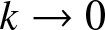 $k \to 0$. In what follows, we use the averaged Lagrangian method to obtain the Whitham modulation equations.
4.1. Averaged conservation laws revisited
Recall that the averaged conservation laws are given by (2.11). Averaging of a  $2\pi$-periodic function
 $F(\theta)$ can now be expressed as
 \begin{equation*}
\overline{F} = \frac{1}{2\pi}\int_0^{2\pi}F(\theta)\,\mathrm{d}\theta =
\frac{|c|k}{2\pi\sqrt{6|\beta|}} \oint
\frac{F(w)}{\sqrt{|G_4(w)|}} \,\mathrm{d}w,
\end{equation*}
in the case of the quartic potential  $\phi(w)$. For example, taking three roots, say
 $w_1$,
 $w_2$,
 $w_3$ incorporating the constraint (3.7), and the averaged particle velocity
 $\overline{v}$ in (3.18) as the modulation parameters
 $\mathbf{W} = (w_1,w_2,w_3,\overline{v})$, eqs. (2.11) are four quasilinear modulation equations for
 $\mathbf{W}$. The first conservation law (2.11a) is
 $\overline{w}_T - \overline{v}_X = 0$, where
 $\overline{w}$ is defined in terms of the roots
 $w_j$ through (3.8) and one of (3.23) or (3.44) or (3.53), respectively. Using
 $\omega = ck$, eq. (3.8) and one of (3.22), (3.43), (3.52) for
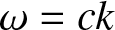
 $k$, the conservation of waves (2.11d) gives another modulation equation. The average velocity (2.11b) and energy (2.11c) equations require further calculation of the density and fluxes. Rather than pursue this further, we instead develop the averaged variational principle.
4.2. Average Lagrangian
Writing the Lagrangian density (2.6) in terms of  $u(x,t)$, we obtain
 \begin{equation}
\mathbb{L}(u_t,u_x,u_{xt}) = \dfrac{1}{2}u_t^2 - \phi(u_x) +
\dfrac{1}{24} u_{xt}^2, \quad \phi'(u_x)=f(u_x)
\end{equation}
and note that it depends only on derivatives of  $u(x,t)$. Furthermore, the periodic travelling wave solutions are obtained for
 $v = u_t$ and
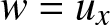 $w = u_x$. Consequently, the most general periodic travelling wave can be written as
 \begin{equation}
u(x,t) = \overline{w} x + \overline{v} t + U(\theta), \quad U(\theta + 2\pi) =
U(\theta), \quad \theta = kx - \omega t .
\end{equation}
The term 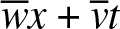 $\overline{w} x + \overline{v} t$ corresponds to the so-called pseudo-phase and enables
 $U(\theta)$ to be
 $2\pi$-periodic.
In the general case (2.3), the Lagrangian density (4.1) is
 \begin{equation}
\mathbb{L}=\dfrac{1}{2}u_t^2-\dfrac{1}{2}u_x^2-\dfrac{1}{3}\alpha
u_x^3-\dfrac{1}{4}\beta u_x^4+\dfrac{1}{24}u_{xt}^2.
\end{equation}
Note that (4.2) implies that  $u_t=\overline{v}-c(w(\theta)-\overline{w})$,
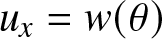 $u_x=w(\theta)$ and
 $u_{xt}=-\omega w'(\theta)$, so that (4.3) can be written solely in terms of
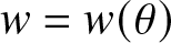 $w = w(\theta)$
 \begin{equation*}
\mathbb{L}=\dfrac{1}{2}\left(\overline{v}-c(w-\overline{w})\right)^2-\dfrac{1}{2}w^2-\dfrac{\alpha}{3}w^3-\dfrac{\beta}{4}
w^4+\dfrac{1}{24}\omega^2(w')^2.
\end{equation*}
Recalling that, in view of (3.4), we have
 \begin{equation}
\dfrac{\omega^2(w')^2}{24}=-\dfrac{\beta}{4}w^4-\dfrac{\alpha}{3}w^3+\dfrac{1}{2}(c^2-1)w^2+\dfrac{1}{2}Aw+\dfrac{1}{2}B,
\end{equation}
we arrive at
 \begin{equation*}
\mathbb{L}=\dfrac{1}{12}\omega^2(w')^2-\left(c^2\overline{w}+\overline{v} c+\dfrac{1}{2}A\right)w+\dfrac{1}{2}\overline{v}^2+\dfrac{1}{2}c^2\overline{w}^2+c\,\overline{v} \,\overline{w}-\dfrac{1}{2}B.
\end{equation*}
Thus, the averaged Lagrangian density is given by
 \begin{equation*}
\mathcal{L}(\overline{w},\overline{v},k,\omega,A,B) = \frac{1}{2\pi} \int_0^{2\pi}
\mathbb{L}(\theta)\,\mathrm{d}\theta
=\dfrac{\omega^2}{12k}\mathcal{W}\left(\dfrac{\omega}{k},A,B\right)+\dfrac{1}{2}\overline{v}^2-\dfrac{\omega^2}{2k^2}\overline{w}^2-\dfrac{1}{2}A\overline{w}-\dfrac{1}{2}B,
\end{equation*}
where
 \begin{equation}
\begin{split}
\mathcal{W}(c,A,B)&=\dfrac{k}{2\pi}\int_0^{2\pi}(w'(\theta))^2d\theta=\dfrac{1}{2\pi}\oint kw'(\theta)dw\\
&=\dfrac{1}{2\pi}\oint \left[\dfrac{12}{c^2}\left(-\dfrac{\beta}{2}w^4-\dfrac{2\alpha}{3}w^3+(c^2-1)w^2+Aw+B\right)\right]^{1/2}dw.
\end{split}
\end{equation}
Here, we used (4.4), and the integration in  $w$ is around the periodic orbit.
The variational equations along with the consistency relations are [Reference Whitham39]
 \begin{equation}
\begin{split}
&\mathcal{L}_A=0, \quad \mathcal{L}_B=0,\\
&\dfrac{\partial}{\partial T}\mathcal{L}_\omega-\dfrac{\partial}{\partial X}\mathcal{L}_k=0, \quad k_T+\omega_X=0,\\
&\dfrac{\partial}{\partial T}\mathcal{L}_{\overline{v}}+\dfrac{\partial}{\partial X}\mathcal{L}_{\overline{w}}=0, \quad \overline{w}_T-\overline{v}_X=0.
\end{split}
\end{equation}
The first equation,  $\mathcal{L}_A=0$, yields
 \begin{equation*}
\overline{w}=\dfrac{c\omega\mathcal{W}_A}{6},
\end{equation*}
which is automatically satisfied because, by (3.5) or (3.13) and (4.5), we have
 \begin{equation*}
\mathcal{W}_A=\begin{cases}\dfrac{6|c|}{2\pi c^2\sqrt{6|\beta|}}\oint\dfrac{w \ dw}{\sqrt{|G_4(w)|}}, & \beta \neq 0 \\
\dfrac{6|c|}{2\pi c^2\sqrt{8|\alpha|}}\oint\dfrac{w \ dw}{\sqrt{|G_3(w)|}}, & \beta=0,
\end{cases}
\end{equation*}
which in either case yields
 \begin{equation*}
\mathcal{W}_A=\dfrac{6}{2\pi c^2k}\int_0^{2\pi} wd\theta=\dfrac{6}{c\omega}\overline{w}.
\end{equation*}
The second equation in (4.6), 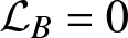 $\mathcal{L}_B=0$, implies that
 \begin{equation*}
k=\dfrac{6}{\mathcal{W}_B c^2},
\end{equation*}
which yields the dispersion relation
 \begin{equation*}
\omega^2=(ck)^2=\dfrac{6}{k \mathcal{W}_B}.
\end{equation*}
We also have the identity
 \begin{equation*}
\mathcal{W}_c = -\frac{1}{c} \mathcal{W} + \frac{12}{\omega}
\overline{w^2} .
\end{equation*}
The remaining four equations in (4.6) yield
 \begin{equation}
\overline{w}_T - \overline{v}_X = 0,
\end{equation}
 \begin{equation}
\overline{v}_T - (c^2\overline{w}+\dfrac{1}{2}A)_X = 0,
\end{equation}
 \begin{equation}
\left(\dfrac{c}{12}\mathcal{W} + c\dfrac{\overline{w^2} - \overline{w}^2}{k}
\right)_T
+\left(c^2\dfrac{\overline{w^2} -
\overline{w}^2}{k}\right )_X = 0 ,
\end{equation}
 \begin{equation}
k_T + \omega_X = 0 .
\end{equation}
Here, (4.7a) and (4.7d) coincide with (2.11a) and (2.11d), respectively, while (4.7b) is equivalent to (2.11b) because, by (3.2), we have
 \begin{equation*}
c^2\overline{w}+\dfrac{1}{2}A=\overline{f(w)+\dfrac{\omega^2}{12}w''(\theta)}=\overline{f(w)}.
\end{equation*}
Equation (4.7c) is the conservation of wave action, which makes (4.7) consistent with (2.11) but, as we will see, remains distinct from the remaining equations in the limit 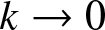 $k \to 0$, whereas eq. (2.11c) becomes redundant with the remaining modulation equations.
Two special limits are of interest. In the solitary-wave limit, we have 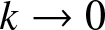 $k \to 0$, and hence
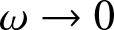 $\omega \to 0$, so that (4.7d) is trivially satisfied. Thus, in this limit, the modulation system consists of three equations (4.7a), (4.7b) and (4.7c) that will be analysed separately for each case. In the harmonic limit, we have
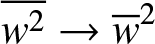 $\overline{w^2} \to \overline{w}^2$ and
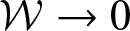 $\mathcal{W} \to 0$, while
 $k$ is nonzero, making the third equation (4.7c) trivial. Thus, the modulation system (4.7) in this limit reduces to three equations, (4.7a), (4.7b) and (4.7d). These equations are given by
 \begin{equation}
\begin{split}
\overline{w}_T-\overline{v}_X&=0,\\
\overline{v}_T-c_s^2(\overline{w})\overline{w}_X&=0,\\
\omega_T+\mathrm{sgn}(\omega)\dfrac{(c_s^2(\overline{w})-\omega^2/12)^{3/2}}{c_s^2(\overline{w})}\omega_X
-\dfrac{(\alpha+3\beta\overline{w})\omega}{c_s^2(\overline{w})}\overline{v}_X&=0,
\end{split}
\end{equation}
where we recall that  $c_s(\overline{w})$ is the sound speed defined in (2.5). We recognize the first two equations as the dispersionless limit of (2.7), as expected. The third equation is found to be equivalent to the modulation equation for linear waves – conservation of waves (4.7d) with
 $\omega = \omega_0(k,\overline{w})$, the linear dispersion relation (2.4), which can be inverted to yield
 \begin{equation*}
k(\omega,\overline{w})=\dfrac{|\omega|}{\sqrt{c_s^2(\overline{w})-\omega^2/12}},
\end{equation*}
where we note that 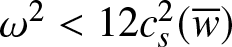 $\omega^2 \lt 12c_s^2(\overline{w})$ by (2.4). The coefficient of
 $\omega_X$ in this equation equals the group velocity
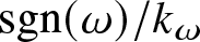 $\mathrm{sgn}(\omega) /k_\omega$, while the coefficient of
 $\overline{v}_X$ is
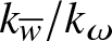 $k_{\overline{w}}/k_\omega$. In both the solitary wave and harmonic limits, the first two mean equations, (4.7a) and (4.7b), decouple from the third.
We will parameterize the Whitham equations (4.7) using a convenient set of modulation variables, i.e., one of  $\mathbf{W}$ in (3.19),
 $\mathbf{A}$ in (3.34),
 $\mathbf{\tilde{A}}$ in (3.38), or
 $\overline{\mathbf{A}}$ in (3.54), depending on the situation. Note that (4.7) have the form
 $\mathbf{P}_T+\mathbf{Q}_X=0$, where
 $\mathbf{P}$ and
 $\mathbf{Q}$ are the density and flux vectors, respectively. For each parametrization
 $\mathbf{r}$, we can find
 $\mathbf{P}(\mathbf{r})$ and
 $\mathbf{Q}(\mathbf{r})$ and rewrite the Whitham modulation equations (4.7) in the hydrodynamic form
 \begin{equation}
\mathbf{r}_T + \mathbb{A}(\mathbf{r})\mathbf{r}_X = \mathbf{0} ,
\end{equation}
where  $\mathbb{A}(\mathbf{r}) = (\partial \mathbf{P}/\partial \mathbf{r})^{-1} \partial \mathbf{Q}/\partial \mathbf{r}$ is obtained using symbolic algebra in Mathematica.
The modulation system  $\mathbf{r}_T + \mathbb{A}(\mathbf{r})\mathbf{r}_X = \mathbf{0}$ has four eigenvalue-eigenvector pairs
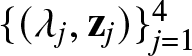 $\{(\lambda_j,\mathbf{z}_j)\}_{j=1}^4$ satisfying
 \begin{equation*}
\mathbb{A}(\mathbf{r}) \mathbf{z}_j(\mathbf{r}) = \lambda_j(\mathbf{r}) \mathbf{z}_j(\mathbf{r}), \quad j = 1, 2,3, 4.
\end{equation*}
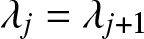
We order the eigenvalues first by their real parts and, for complex conjugate eigenvalues, then by their imaginary parts. We say that the modulation system is strictly hyperbolic if  $\lambda_j \le \lambda_{j+1} \in \mathbb{R}$ and
 $\lambda_j = \lambda_{j+1}$ if and only if the
 $j^{\rm th}$ and
 $(j+1)^{\rm th}$ modulation equation are equivalent. Here we use an extended definition of strict hyperbolicity (see, e.g., [Reference Levermore30]) in which merged characteristic velocities correspond to a reduction in order of the modulation system. For example, this is precisely the case in the solitary wave and harmonic limits of (4.7), where either the conservation of waves (4.7d) or conservation of wave action (4.7c) are identically zero in the respective limits. Both limits thus maintain strict hyperbolicity of the modulation system provided that
 $c_s^2(\overline{w})=f'(\overline{w}) \gt 0$. The
 $j^{\rm th}$ characteristic field is said to be genuinely nonlinear if [Reference Lax29]
 \begin{equation}
\mu_j(\mathbf{r}) = \nabla_{\mathbf{r}} \lambda_j(\mathbf{r}) \cdot \mathbf{z}_j(\mathbf{r}) \ne 0 , \quad j = 1,2,3,4.
\end{equation}
Together, strict hyperbolicity and genuine nonlinearity characterize the convexity of the system.
In particular, the system of the first two mean equations in (4.8), which decouples from the remaining equation in the harmonic and solitary-wave limits, has eigenvalues  $\lambda_{1,2}=\mp c_s(\overline{w})$ and the corresponding eigenvectors
 $\mathbf{z}_{1,2}=(1,\pm c_s(\overline{w}))^T$, yielding
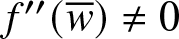
 $\mu_{1,2}=\mp f''(\overline{w})/(2\sqrt{f'(\overline{w})})$. This subsystem is strictly hyperbolic as long as
 $c_s^2(\overline{w})=f'(\overline{w}) \gt 0$ and it is genuinely nonlinear when
 $f''(\overline{w}) \neq 0$.
Considering now the harmonic-limit system (4.8), we find that the eigenvalues are
 \begin{equation*}
\lambda_1=-c_s(\overline{w}), \quad \lambda_2= \mathrm{sgn}(\omega)\dfrac{(c_s^2(\overline{w})-\omega^2/12)^{3/2}}{c_s^2(\overline{w})}, \quad \lambda_3=c_s(\overline{w}),
\end{equation*}
and the corresponding eigenvectors are
 \begin{equation*}
\begin{split}
&\mathbf{z}_1=\left(1,c_s(\overline{w}),\dfrac{(\alpha+3\beta\overline{w})c_s(\overline{w})\omega}{\mathrm{sgn}(\omega)
(c_s^2(\overline{w})-\omega^2/12)^{3/2}+c_s^3(\overline{w})}\right)^T,
\quad \mathbf{z}_2=(0,0,1)^T, \\
&\mathbf{z}_3=\left(1,-c_s(\overline{w}),-\dfrac{(\alpha+3\beta\overline{w})c_s(\overline{w})\omega}{\mathrm{sgn}(\omega)(c_s^2(\overline{w})-\omega^2/12)^{3/2}-c_s^3(\overline{w})}\right)^T,
\end{split}
\end{equation*}
yielding
 \begin{equation*}
\mu_1=-\dfrac{f''(\overline{w})}{2\sqrt{f'(\overline{w})}}, \quad \mu_2=-\dfrac{(f'(\overline{w})-\omega^2/12)^{1/2}}{4f'(\overline{w})}|\omega|,
\quad \mu_3=\dfrac{f''(\overline{w})}{2\sqrt{f'(\overline{w})}} .
\end{equation*}
Since the harmonic wave frequency is bounded from above (2.4), the system is strictly hyperbolic when  $c_s^2(\overline{w}) = f'(\overline{w}) \gt 0$ and genuinely nonlinear when
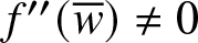 $f''(\overline{w}) \neq 0$ and
 $\omega \neq 0$. In particular, in the case
 $(\alpha,\beta)=(1,0)$ considered below, the harmonic limit is convex (strictly hyperbolic and genuinely nonlinear) when
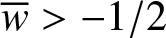 $\overline{w} \gt -1/2$ and
 $\omega \neq 0$. For cubic nonlinearity with
 $(\alpha,\beta)=(0,1)$, the harmonic limit system is always strictly hyperbolic, while in the case
 $(\alpha,\beta)=(0,-1)$ strict hyperbolicity requires
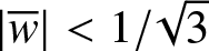 $|\overline{w}| \lt 1/\sqrt{3}$. In both cases, we must have
 $\omega \neq 0$ and
 $\overline{w} \neq 0$ for genuine nonlinearity.
4.3. Quadratic nonlinearity:
$(\alpha,\beta) = (1,0)$

We now consider the special case of  $(\alpha,\beta) = (1,0)$. Note that, if
 $\beta = 0$, we can set
 $\alpha = 1$ without loss of generality using the transformation
 $\alpha u \to u$, as noted in Section 2.1. We wish to express the Whitham eqs. (4.7) in terms of the parameter set
 $\mathbf{W} = (w_1,w_2,w_3,\overline{v})^T$. For this, we will need to calculate
 \begin{equation*}
\begin{split}
\mathcal{W} &= \frac{1}{2\pi} \sqrt{\frac{8}{c^2}} \oint
\sqrt{-G_3(w)}\,\mathrm{d} w = \frac{1}{\pi}\sqrt{\frac{8}{c^2}}
\int_{w_2}^{w_3} \sqrt{-G_3(w)}\,\mathrm{d} w, \\
\overline{w^2} &= \frac{1}{2\pi} \int_0^{2\pi}
w^2(\theta)\,\mathrm{d}\theta = \frac{1}{2\pi} \sqrt{\frac{\omega^2}{8}} \oint
\frac{w^2}{\sqrt{-G_3(w)}}\,\mathrm{d}w =
\frac{1}{\pi} \sqrt{\frac{\omega^2}{8}}
\int_{w_2}^{w_3}
\frac{w^2}{\sqrt{-G_3(w)}}\,\mathrm{d}w .
\end{split}
\end{equation*}
Evaluating the elliptic integrals, we obtain [Reference Byrd and Friedman4]
 \begin{equation*}
\mathcal{W} = \frac{4\sqrt{2}}{15\pi |c|}
\frac{(w_3-w_2)(w_2-w_1)^2}{\sqrt{w_3-w_1}}
\frac{2(1-m+m^2) E(m) -
(2-m)(1-m)K(m)}{m(1-m)^2}
\end{equation*}
and
 \begin{align*}
\begin{split}
\overline{w^2} &= \frac{|\omega|}{3\sqrt{2}\pi(m-1)^2\sqrt{w_3-w_1}}
\biggl\{2(w_2-w_1)\biggl ( (1-2m)w_1+(2-m)w_2 \biggr )E(m)\\
& + (m-1)\left((3m-2)w_1^2-2 w_1w_2 + w_2^2 \right)K(m)\biggr\}.
\end{split}
\end{align*}
Using equations (3.15), (3.16), (3.51), (3.52), (3.53) with  $\alpha=1$, we obtain
 \begin{equation}
\begin{split}
A &= - \frac{2}{3}(w_1 w_2 + w_1 w_3 + w_2 w_3), \\
c^2 &= 1 + \frac{2}{3}(w_1+w_2+w_3) , \quad \omega = c k, \\
k &= \dfrac{\sqrt{2}\pi}{|c|K(m)}\sqrt{w_3-w_1}, \quad m =
\frac{w_3-w_2}{w_3-w_1} , \\
\overline{w} &= w_1+(w_3-w_1)\dfrac{E(m)}{K(m)}.
\end{split}
\end{equation}
Consequently, we have expressed each density and flux of the Whitham equations (4.7) in terms of the parameters  $\mathbf{W}$ in (3.19).
4.3.1. Solitary-wave limit
We now pass to the solitary-wave limit  $w_2 \to w_1$ in the Whitham equations (4.7). The terms in the wave-action density eq. (4.7c) exhibit the limits
 \begin{equation*}
\begin{split}
\lim_{w_2 \to w_1} \frac{c}{12} \mathcal{W}
&= \frac{\sqrt{2}\mathrm{sgn}(c)}{2\pi} \frac{4}{45} (w_3-w_1)^{5/2}, \\
\lim_{w_2 \to w_1} c \frac{\overline{w^2} - \overline{w}^2}{k}
&= \frac{\sqrt{2}\mathrm{sgn}(c)}{2\pi} \frac{2}{3} c^2(w_3 - w_1)^{3/2} , \\
\lim_{w_2 \to w_1} \overline{w} &= w_1 , \\
\lim_{w_2 \to w_1} \overline{w^2} &= w_1^2 , \\
\lim_{w_2 \to w_1} c^2 &= 1 + \frac{2}{3}(2 w_1 + w_3).
\end{split}
\end{equation*}
Since the solitary wave amplitude is  $a = w_3 - w_1$ (cf. Section 3.3), we can express the above quantities in terms of
 $\overline{\mathbf{A}} =(1,a,\overline{v},\overline{w})^T$ to obtain
 \begin{equation}
\overline{w}_T - \overline{v}_X = 0 ,
\end{equation}
 \begin{equation}
\overline{v}_T - f(\overline{w})_X = 0 ,
\end{equation}
 \begin{equation}
\left ((1+2\overline{w})a^{3/2} + \tfrac{4}{5} a^{5/2} \right
)_T + \left ( c \left ( (1+2\overline{w})a^{3/2} +
\tfrac{2}{3} a^{5/2} \right ) \right )_X = 0 ,
\end{equation}
where
 \begin{equation*}
c^2 = 1 + 2\overline{w} + \frac{2}{3} a , \quad f(\overline{w}) = \overline{w} + \overline{w}^2 .
\end{equation*}
 $2\pi/(\sqrt{2}\mathrm{sgn}(c))$ to simplify the expression. We recognize eqs. (4.12a) and (4.12b) as the dispersionless limit of eq. (2.7) and eq. (4.12c) is the equation for the solitary-wave amplitude field
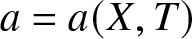 $a = a(X,T)$. Expanding eq. (4.12c) and replacing
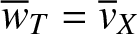 $\overline{w}_T =
\overline{v}_X$, we obtain
 \begin{equation}
a_T + c \,a_X + \frac{4 a}{3(1+2\overline{w}+\frac{4}{3}a)} \overline{v}_X +
\frac{2 c a}{1+2\overline{w}+\frac{4}{3}a} \overline{w}_X
= 0 .
\end{equation}
Because it is decoupled from the other equations (4.12a), (4.12b), the characteristic velocity for (4.13) is  $\lambda=c$, as it should be in the solitary-wave limit.
Equation (4.12) exhibits the ordered characteristic velocities (for the branch of fast waves with  $c \gt 0$)
 \begin{equation*}
\lambda_1 = -\sqrt{1+2\overline{w}}, \quad \lambda_2 = \sqrt{1+2\overline{w}}, \quad
\lambda_3 = c = \sqrt{1 + 2\overline{w} + \tfrac23 a} .
\end{equation*}
The corresponding eigenvectors are
 \begin{equation*}
\mathbf{z}_1 =
\begin{bmatrix}
1 \\ \sqrt{1+2\overline{w}} \\ -
\frac{1+2\overline{w}+2a+\sqrt{(1+2\overline{w})(1+2\overline{w}+\frac{2}{3}a)}}{1+2 \overline{w} +
\frac{4}{3}a}
\end{bmatrix}, \quad
\mathbf{z}_2 =
\begin{bmatrix}
1 \\ \sqrt{1+2\overline{w}} \\ -
\frac{1+2\overline{w}+2a-\sqrt{(1+2\overline{w})(1+2\overline{w}+\frac{2}{3}a)}}{1+2 \overline{w} +
\frac{4}{3}a}
\end{bmatrix}, \quad
\mathbf{z}_3 =
\begin{bmatrix}
0 \\ 0 \\ 1
\end{bmatrix} .
\end{equation*}
4.3.2. Convexity
We first examine the convexity (hyperbolicity, genuine nonlinearity) of the Whitham equations in the solitary-wave limit (4.12). The mean lower bound 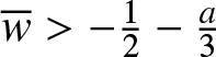 $\overline{w} \gt -\frac{1}{2}-\frac{a}{3}$ for solitary waves (recall (3.56)) ensures that
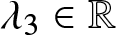 $\lambda_3 \in \mathbb{R}$ but it does not preclude the possibility of complex characteristic velocities
 $\lambda_1$ and
 $\lambda_2$. Thus, to ensure strict hyperbolicity, we further require
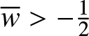 $\overline{w} \gt -\frac{1}{2}$ and
 $a \gt 0$. To assess genuine nonlinearity, we compute
 \begin{equation*}
\begin{split}
\mu_j &= \nabla \lambda_j \cdot \mathbf{z}_j = \partial_{\overline{w}}
\lambda_j = \frac{1}{\lambda_j} \ne 0, \quad j = 1,2, \\
\mu_3 &= \nabla \lambda_3 \cdot \mathbf{z}_3 = \partial_a
\lambda_3(a,\overline{w}) = \frac{1}{3
\lambda_3} \ne 0 .
\end{split}
\end{equation*}
Thus, the solitary-wave modulation system is genuinely nonlinear, provided it is strictly hyperbolic.
We now examine the convexity of the full Whitham system (4.7) by numerically computing the eigenvalues and eigenvectors of the modulation matrix  $\mathbb{A}(\mathbf{r})$ in (4.9) as
 $\overline{\mathbf{A}}$ is varied. Recalling the admissibility criteria (3.57), (3.58), we will study convexity in two separate regimes:
(a)
$\overline{E}_a^{(\rm a)}$:
$\overline{w} \gt -\frac{1}{2}$,
$0 \lt a \lt a_{\rm max}$, and
$0 \lt m \lt 1$,(b)
$\overline{E}_a^{(\rm b)}$:
$\overline{w}_{\rm min}(m,a) \lt \overline{w}$,
$a \gt 0$, and
$m_* \lt m \lt 1$,

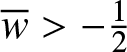






where  $\overline{w}_{\rm min}$ is given by (3.55),
 $a_{\rm max}$ is defined in (3.59) and
 $m_* \approx 0.96115$ satisfies
 $3\ E(m_*) - (2-m_*)K(m_*) = 0$. For case (a), we introduce the change of variables
 \begin{equation*}
\mathrm{(a)} \quad u \to (1+2\overline{w}) u + \overline{v} t + \overline{w} x, \quad t \to \frac{t}{\sqrt{1+2\overline{w}}},
\quad \overline{w} \gt -\frac{1}{2},
\end{equation*}
to eq. (2.1), leaving it unchanged since 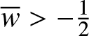 $\overline{w} \gt -\tfrac12$. Consequently, in this case, we will set
 $\overline{v} = \overline{w} = 0$ without loss of generality and consider variation of the remaining two modulation parameters
 $0 \lt m \lt 1$,
 $0 \lt a \lt a_{\rm max}(m,\overline{w} = 0)$. For case (b), we note that eq. (2.1) is invariant under the alternative change of variables
 \begin{equation*}
\mathrm{(b)} \quad u \to \frac{u}{a} + \overline{v} t + \left ( \frac{1}{2a} - \frac{1}{2} \right
) x, \quad t \to \sqrt{a} t,
\quad a \gt 0,
\end{equation*}
Now, we will set  $a = 1$ without loss of generality and consider convexity when
 $m_* \lt m \lt 1$ and
 $\overline{w} \gt \overline{w}_{\rm min}(m,a=1)$.
Figure 3 depicts the (white) region of strict hyperbolicity when 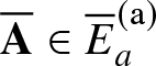 $\overline{\mathbf{A}} \in \overline{E}_a^{(\rm a)}$. We find that
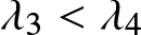 $\lambda_3 \lt \lambda_4$ are real and distinct for all computed admissible parameter values. There exists a greyscale region in which the modulations exhibit complex conjugate characteristic velocities
 $\lambda_1$ and
 $\lambda_2$. Such regions correspond to modulational instability of the underlying periodic travelling wave [Reference Whitham39]. At the boundaries of these regions,
 $\lambda_1 = \lambda_2 \in \mathbb{R}$. The coalescence of two characteristics coincides with loss of genuine nonlinearity, so
 $\mu_1 = \mu_2 = 0$ also. The smallest values of
 $m$ and
 $a$ where complex characteristics occur are depicted as black dots.
Hyperbolicity of the regularized Boussinesq–Whitham equations for  $(\alpha,\beta) = (1,0)$ (case III), quadratic interaction force with
 $\overline{\mathbf{A}} = (m,a,\overline{v}=0,\overline{w}=0) \in \overline{E}_a^{(a)}$: Strict hyperbolicity (white region). Greyscale is the magnitude of the imaginary part of
 $\lambda_2$ where the system is not hyperbolic. Periodic travelling waves do not exist in the inadmissible pink region. Black dots depict points corresponding to the values
 $(m,a) \in \{(0.83,2.69),~(0.89,2.27)\}$ in (a) and
 $(m,\omega) = (0.83,3.41)$ in (b) where complex characteristic velocities are first encountered. The solid black curves correspond to parameters where the second characteristic field loses genuine nonlinearity,
 $\mu_2 = \nabla \lambda_2 \cdot \mathbf{z}_2 = 0$, and
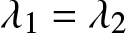 $\lambda_1 = \lambda_2$ at the boundary of the non-hyperbolic region. Panels (a) and (b) are equivalent under the transformation (3.60).

Figure 3 Long description
The image A showing a contour plot of Im lambda 2 as a function of m and a. The x-axis label is m, with no unit specified, ranging from 0 to 1. The y-axis label is a, with no unit specified, ranging from 0 to 5. A vertical scale bar is labeled Im lambda 2, with no unit specified, ranging from 0 to 0.7. A boundary curve separates a large region where Im lambda 2 is shown as 0 from a region above the curve. The boundary passes through approximately (m equals 0, a equals 0), then rises with m. At m equals 0.2 the boundary is near a about 0.3. At m equals 0.4 the boundary is near a about 0.8. At m equals 0.6 the boundary is near a about 1.6. At m equals 0.8 the boundary is near a about 3.0. The boundary reaches the upper edge near m between 0.85 and 0.9. For m between about 0.8 and 1, a shaded lobe indicates Im lambda 2 greater than 0. The lobe spans roughly a from about 2.3 up to 5. Within this lobe, the darkest shading occurs near m close to 1 and a near 4 to 5, approaching the upper scale value 0.7. A closed contour loop is visible inside the lobe. The image B showing a contour plot of Im lambda 2 as a function of m and a. The x-axis label is m, with no unit specified, ranging from 0 to 1. The y-axis label is a, with no unit specified, ranging from 0 to 4. A vertical scale bar is labeled Im lambda 2, with no unit specified, ranging from 0 to 1.5. A boundary curve runs across the plot at a between about 3.4 and 3.6 for m from 0 to about 0.8, then bends upward for m above about 0.8 and approaches a near 4 as m approaches 1. For a below this boundary, most of the plotted area corresponds to Im lambda 2 shown as 0. For m close to 1, a shaded region indicates Im lambda 2 greater than 0 over a range from about 2.5 up to 4. The shading increases toward m equals 1, with the darkest values near m close to 1 and a near 4, approaching the upper scale value 1.5. A contour line within this region curves from about (m about 0.85, a about 3.6) toward (m close to 1, a about 2.7).
We also compute the quantities  $\mu_j$ in (4.10) in the strictly hyperbolic region and find that only
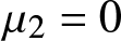 $\mu_2 = 0$ (i.e.,
 $\mu_1 \ne 0$, so $\lambda_1 \ne \lambda_2$) on a curve bifurcating from
 $(a,m) = (0,0)$ or
 $(\omega,m) = (\sqrt{12},0)$. The curve is depicted in Fig. 3. Nonzero
 $\mu_j$ is a necessary monotonicity condition for the existence of a
 $j$-integral curve in which
 $\mathbf{r}'(\alpha) = \mathbf{z}_j(\mathbf{r}(\alpha))$ where
 $\alpha$ evolves along the characteristic
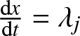 $\frac{\mathrm{d}x}{\mathrm{d}t} = \lambda_j$:
 $\alpha_t + \lambda_j(\mathbf{r}(\alpha)) \alpha_x = 0$. Simple waves are used in the solution of the Riemann problem consisting of step initial conditions at the origin. The short-wave limit (
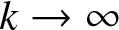 $k \to \infty$) occurs when
 $a$ approaches the pink admissibility boundary (
 $a \to a_{\rm max}$). At this boundary, the modulation matrix
 $\mathbb{A}$ exhibits a double zero eigenvalue and two real, oppositely signed eigenvalues.
Figure 4 depicts hyperbolicity for case (b) where we normalize the amplitude to  $a = 1$ and require
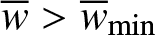 $\overline{w} \gt \overline{w}_{\rm min}$,
 $m_* \le m \lt 1$. We observe that the system is hyperbolic when
 $\overline{w}$ is sufficiently large. The depicted results are consistent with the solitary-wave limit (4.12) that is strictly hyperbolic for
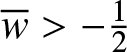 $\overline{w} \gt -\frac{1}{2}$. The upper dashed curve in Figure 4 where
 $\lambda_1 = \lambda_2$ limits to
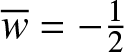 $\overline{w} = -\frac{1}{2}$ as
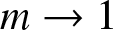 $m \to 1$ but the approach is very sharp due to the logarithmic approach of
 $\overline{w}$ to
 $-\frac{1}{2}$ because
 $K(m) \sim -1/\log(1-m)$ in the mean equation (4.11) as
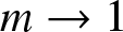 $m \to 1$. In a similar manner, the lower dashed curve in Fig. 4 at the boundary of the admissible region also sharply limits to
 $\overline{w} = \overline{w}_{\rm min}(a=1,m=1) = -\frac{5}{6}$ as
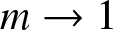 $m \to 1$. This demonstrates that the region in Fig. 4 where hyperbolicity is lost bifurcates from the segment
 $-\frac{5}{6} \lt \overline{w} \lt -\frac{1}{2}$ for
 $m = 1$, which is denoted by the red segment.
Hyperbolicity of the regularized Boussinesq–Whitham equations for case III, quadratic interaction force with  $\overline{\mathbf{A}} = (m,a=1,\overline{v}=0,\overline{w}) \in \overline{E}_a^{(b)}$: Strict hyperbolicity (white region). Greyscale is the magnitude of the imaginary part of
 $\lambda_2$ where the system is not hyperbolic. At
 $m = m_* \approx 0.96115$, we find that for
 $\overline{w} \gt -0.298$, the system is strictly hyperbolic. The dashed curves correspond to the boundary of the non-hyperbolic region where
 $\lambda_1 = \lambda_2$, so that
 $\mu_1 = \mu_2 = 0$ there also. Periodic travelling waves do not exist in the inadmissible pink region. The red segment at
 $m = 1$ corresponds to the region of non-hyperbolicity of the solitary-wave limiting system (4.12).

4.4. Cubic nonlinearity with
$(\alpha,\beta) = (0,1)$

We now consider the case of cubic  $f(w)$ with
 $(\alpha,\beta)=(0,1)$, to which, as we discussed in Section 2.1, case I in Section 3.1 can be reduced upon a proper rescaling. As before, we need to compute
 $\mathcal{W}$ and
 $\overline{w^2}$ that are given by
 \begin{equation*}
\mathcal{W} = \frac{1}{2\pi} \sqrt{\frac{6}{c^2}} \oint \sqrt{-G_4(w)}\, \mathrm{d} w, \quad
\overline{w^2} = \frac{1}{2\pi} \sqrt{\frac{\omega^2}{6}} \oint \dfrac{w^2}{\sqrt{-G_4(w)}}\, \mathrm{d} w.
\end{equation*}
Recall that in this case we have two families of periodic solutions related by the symmetry transformation (3.33) with  $\alpha=0$ and
 $\beta=1$. Thus, it suffices to consider the first solution family (3.21). We have
 \begin{equation}
\begin{split}
&w_1 + w_2 + w_3 + w_4 = 0,\\
& A = \frac{1}{2}(w_1w_2w_3 + w_1 w_2 w_4+w_1 w_3 w_4+w_2 w_3
w_4),\\
&c^2 = 1 - \frac{1}{2} ( w_1 w_2 + w_1 w_3 + w_1 w_4 + w_2 w_3 +
w_2 w_4 + w_3 w_4 ),\\
&k = \frac{\pi}{K(m)} \sqrt{\frac{3}{2c^2}(w_4-w_2)(w_3-w_1)}, \quad \omega=ck,\\
&m = \frac{(w_4-w_3)(w_2-w_1)}{(w_4-w_2)(w_3-w_1)},
\end{split}
\end{equation}
where we used (3.7), (3.8), (3.11), (3.21) and (3.22).
To find  $\mathcal{W}$ and
 $\overline{w^2}$ we use
 \begin{equation*}
\begin{split}
\mathcal{W} &= \frac{1}{\pi} \sqrt{\frac{6}{c^2}} \int_{w_1}^{w_2} \sqrt{(w-w_1)(w_2-w)(w_3-w)(w_4-w)}\, \mathrm{d} w, \\
\overline{w^2} &= \frac{1}{\pi} \sqrt{\frac{\omega^2}{6}} \int_{w_1}^{w_2} \dfrac{w^2\,\mathrm{d} w}{\sqrt{(w-w_1)(w_2-w)(w_3-w)(w_4-w)}}.
\end{split}
\end{equation*}
Evaluation of the elliptic integrals yields [Reference Byrd and Friedman4]
 \begin{equation*}
\begin{split}
\mathcal{W}&=\dfrac{(w_2 - w_1)^2 (w_3-w_1)^{1/2} (w_4 -w_1)^2}{4|c| \sqrt{6}\pi
n^3 (1 + n)^2 (n +
m)^2 (w_4-w_2)^{3/2}} \bigg\{n \bigg(3 n^4 + 3 m^2 + 4 n^3 (1 + m)\\
&+ 4 n m (1 + m) + 2 n^2 (2 + m + 2 m^2)\bigg) E(m) \\
&- (n + m) \bigg(3 n^4 - 4 n^2 (m-1) - 3 m^2 -
6 n m^2 + 2 n^3 (2 + m)\bigg) K(m) \\
&+ 3 (n^2 - m) (2 n + n^2 + m) (n^2 + m +
2 n m) \Pi(-n, m)\bigg\}
\end{split}
\end{equation*}
and
 \begin{equation}
\begin{split}
\overline{w^2}&=\dfrac{\sqrt{2}w_4^2|\omega|}{\sqrt{3}\pi \sqrt{(w_3 - w_1) (w_4 - w_2)}}\bigg\{K(m) + 2\left(\dfrac{w_1}{w_4}-1\right)\Pi(-n,m)\\
&+ \dfrac{(w_4 -w_1)^2}{2 (1 +n) (n + m) w_4^2} \bigg(n E(m) - (n + m) K(m) \\
&+ \bigg(n^2 + 3 m +
2 n (1 + m) \bigg) \Pi(-n, m)\bigg)\bigg\},
\end{split}
\end{equation}
where we recall that  $m$ and
 $n$ are given in (3.21) and satisfy (3.24) and (3.25) in the case of real and complex
 $w_{3,4}$, respectively.
4.4.1. Solitary-wave limit
Recall that in the solitary-wave limit  $w_2 \to w_3$ (
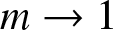 $m \to 1$), the solutions approach the two-parameter family (3.28) with amplitude
 $a=w_3-w_1$, background
 $\overline{w}=w_3$ and velocity (3.29). In this limit, we obtain
 \begin{equation*}
\begin{split}
\lim_{w_2 \to w_3}\dfrac{c}{12}\mathcal{W}&=\dfrac{\text{sgn}(c)}{\pi\sqrt{6}}\bigg\{\dfrac{1}{6}\sqrt{a(a-4\overline{w})}(a^2 - 4 a \overline{w} + 6 \overline{w}^2)\\
&+(a -2 \overline{w})^2 \overline{w} \arctan\sqrt{\dfrac{a}{a - 4\overline{w}}}\biggl\},\\
\lim_{w_2 \to w_3}c\dfrac{\overline{w^2}-\overline{w}^2}{k}&=\dfrac{c^2\text{sgn}(c)}{\pi\sqrt{6}} \bigg\{\sqrt{a(a-4\overline{w})}+4\overline{w}\arctan\sqrt{\dfrac{a}{a - 4\overline{w}}}\bigg\},\\
\lim_{w_2 \to w_3}\overline{w^2} &= \overline{w}^2, \quad \lim_{w_2 \to w_3}c^2=1+3\overline{w}^2+\dfrac{1}{2}a(a-4\overline{w}),
\end{split}
\end{equation*}
where we recall that either 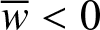 $\overline{w} \lt 0$ and
 $a \gt 0$ or
 $a \gt 4 \overline{w} \gt 0$ by (3.30) with
 $\alpha=0$. In this limit, the Whitham modulation equations (4.7) with
 $f(w)=w+w^3$ become
 \begin{equation}
\begin{split}
\overline{w}_T-\overline{v}_X&=0,\\
\overline{v}_T-(1+3\overline{w}^2)\overline{w}_X&=0,\\
a_T+c\,a_X+c\,\dfrac{g(a,\overline{w})}{d(a,\overline{w})}\overline{w}_X+\dfrac{h(a,\overline{w})}{d(a,\overline{w})}\overline{v}_X&=0,
\end{split}
\end{equation}
where
 \begin{equation}
\begin{split}
g(a,\overline{w})&=-\sqrt{a(a-4\overline{w})}(2 + 4 a^2 - 19 a \overline{w} + 24 \overline{w}^2)\\
&+2 (2 + (a - 6 \overline{w}) (a - 4 \overline{w})) (a - 2 \overline{w})\arctan\sqrt{\dfrac{a}{a - 4 \overline{w}}},\\
h(a,\overline{w})&=-\sqrt{a(a-4\overline{w})} (2 + 4 a^2 - 19 a \overline{w} + 24 \overline{w}^2)\\
&+ (4 + 3 (a - 4 \overline{w})^2) (a - 2 \overline{w}) \arctan\sqrt{\dfrac{a}{a - 4 \overline{w}}},\\
d(a,\overline{w})&=\sqrt{a(a-4\overline{w})} (1 + 2 a^2 - 8 a \overline{w} + 9 \overline{w}^2) +6 (a - 2 \overline{w})^2 \overline{w} \arctan\sqrt{\dfrac{a}{a - 4 \overline{w}}}.
\end{split}
\end{equation}
The ordered characteristic velocities (for the fast waves with  $c \gt 0$) are
 \begin{equation}
\lambda_1 = -\sqrt{1+3\overline{w}^2}, \quad \lambda_2 = \sqrt{1+3\overline{w}^2}, \quad
\lambda_3 = c =
\sqrt{1+3\overline{w}^2+\dfrac{1}{2}a(a-4\overline{w})} .
\end{equation}
The associated eigenvectors are
 \begin{equation}
\mathbf{z}_j =
\begin{bmatrix}
1 \\ -\lambda_j \\ \frac{\lambda_j h(a,\overline{w}) - \lambda_3
g(a,\overline{w})}{d(a,\overline{w})(\lambda_3 - \lambda_j)}
\end{bmatrix}
, \quad j = 1,2, \quad \mathbf{z}_3 =
\begin{bmatrix}
0 \\ 0 \\ 1
\end{bmatrix} .
\end{equation}
In the limit  $w_2 \to w_3 \to w_4$ the solitary waves reduce to the one-parameter family (3.31) with background
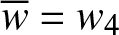 $\overline{w}=w_4$, amplitude
 $a=w_4-w_1=4\overline{w}$, where the second equality follows from the first equation in (4.14), and velocity (3.32), yielding
 \begin{equation*}
\begin{split}
\lim_{w_2 \to w_3 \to w_4}\dfrac{c}{12}\mathcal{W}&=\dfrac{\text{sgn}(c)}{32\sqrt{6}}a^3, \quad
\lim_{w_2 \to w_3 \to w_4}c\dfrac{\overline{w^2}-\overline{w}^2}{k}=\dfrac{c^2\text{sgn}(c)}{2\sqrt{6}}a,\\
\lim_{w_2 \to w_3 \to w_4}\overline{w^2} &= \overline{w}^2, \quad \lim_{w_2 \to w_3 \to w_4}c^2=1+\dfrac{3}{16}a^2=c_s^2(\overline{w}).
\end{split}
\end{equation*}
In this case, the third equation in (4.16) decouples from the first two and becomes  $a_T+c\,a_X=0$, which for
 $c \gt 0$ is equivalent to the fast characteristic family in the first two equations of (4.16), i.e.,
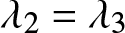 $\lambda_2 = \lambda_3$. Thus, the algebraic solitary wave (3.31) with
 $c=c_s(\overline{w}) \gt 0$ (
 $c=-c_s(\overline{w}) \lt 0$) moves with the fast (slow) characteristic velocity of mean evolution.
4.4.2. Convexity
Here, we examine the convexity of the Whitham modulation equations using various means. First, we consider convexity of the solitary-wave modulation system (4.16) analytically and then proceed to assess the convexity of the full modulation equations (4.7) by numerically evaluating the eigenstructure of the modulation matrix  $\mathbb{A}$ in (4.9).
The solitary-wave existence conditions  $\overline{w} \lt 0$ and
 $a \gt 0$ or
 $a \gt 4\overline{w} \gt 0$ in eq. (3.30) with
 $\alpha=0$ for the first solitary-wave family (3.28) imply real characteristic velocities (4.18). When
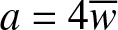 $a = 4 \overline{w}$, either
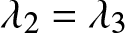 $\lambda_2 = \lambda_3$ (for
 $c \gt 0$) or
 $\lambda_1 = c = \lambda_2 = -\sqrt{1+3\overline{w}^2}$ (for
 $c \lt 0$). This case corresponds to the algebraic solitary wave, whose modulation is equivalent to the fast or slow mean modulation. Consequently, the solitary-wave modulation system (4.16) with (4.17) is strictly hyperbolic.
From (4.18) and (4.19) it follows that the genuine nonlinearity conditions (4.10) are
 \begin{align*}
\mu_j &= \nabla \lambda_j \cdot \mathbf{z}_j = \partial_{\overline{w}}
\lambda_j = \frac{3
\overline{w}}{\lambda_j} \ne 0, \quad j = 1,2, \\
\mu_3 &= \nabla \lambda_3 \cdot \mathbf{z}_3 = \partial_a
\lambda_3(a,\overline{w}) = \frac{a - 2\overline{w}}{2
\lambda_3} \ne 0 .
\end{align*}
Consequently, the solitary-wave modulation system (4.16) with (4.17) loses genuine nonlinearity in both of the mean modulation characteristic families at an inflection point of the interaction force  $f''(\overline{w}) = 3 \overline{w} = 0$. Since either
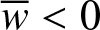 $\overline{w} \lt 0$ and
 $a \gt 0$ or
 $a \gt 4 \overline{w} \gt 0$ for solitary wave existence, we have
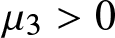 $\mu_3 \gt 0$.
Thus, the modulation system in the solitary-wave limit is strictly hyperbolic for all parameter values and loses genuine nonlinearity when  $\overline{w} = 0$. Recall that the same is true for the harmonic limit in this case. Since
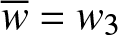 $\overline{w} = w_3$,
 $a = w_3 - w_1$ and
 $w_4 = -2w_3-w_1$, the loss of genuine nonlinearity occurs precisely when
 $n = (w_3-w_1)/(w_4-w_3) = 1$.
For the full Whitham modulation system in the case of real roots  $w_j$, we find that the equations are strictly hyperbolic for
 $n \gt 0$,
 $0 \lt m \lt 1$. Figure 5 depicts curves in the
 $m$-
 $n$ plane with fixed
 $a$ where the modulation system loses genuine nonlinearity in one of the first two characteristic families. These curves bifurcate from the
 $m = 1$ solitary-wave limit at
 $n = 1$, the inflection point of the interaction force
 $\overline{w} = 0$ where the solitary wave limiting system (4.16) loses genuine nonlinearity. Since the modulated periodic travelling wave amplitude is held constant, the limit
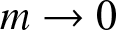 $m \to 0$ corresponds to the trigonometric wave limit where
 $w_3 \to w_4$.
Convexity of the Whitham modulation equations for  $(\alpha,\beta) = (0,1)$ (case I) with real roots
 $w_j$. For each fixed amplitude
 $a$, the solid (dashed) curves correspond to the loss of genuine nonlinearity
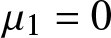 $\mu_1 = 0$ (
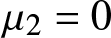 $\mu_2 = 0$) bifurcating from the point
 $(n,m) = (1,1)$ where the solitary-wave limiting system loses genuine nonlinearity at
 $\overline{w} = 0$.

Figure 5 Long description
The plots depict n versus m for different fixed values of a, illustrating the loss of genuine nonlinearity. The x-axis is labeled m, ranging from 0 to 1. The y-axis is labeled n, ranging from 0 to 2.5. Units are not specified. Each plot contains a solid and a dashed curve. The solid curve represents one characteristic family, while the dashed curve represents another. For a equals 0.2, the dashed curve starts at n approximately 0.85 at m equals 0, dips slightly and ends at n 1.0 at m equals 1. The solid curve appears from m approximately 0.75, decreasing from n 2.5 to n 1.3 at m equals 1. For a equals 0.5, the dashed curve decreases from n 1.6 at m equals 0 to n 1.1 at m equals 1. The solid curve starts around m 0.6, decreasing from n 2.5 to n 1.2 at m equals 1. For a equals 1, the dashed curve decreases from n 2.5 at m equals 0 to n 1.2 at m equals 1. The solid curve starts around m 0.45, decreasing to n 1.1 at m equals 1. For a equals 2, the dashed curve decreases from n 2.5 at m approximately 0.25 to n 1.2 at m equals 1. The solid curve starts around m 0.5, decreasing to n 1.1 at m equals 1. The plots show how the curves shift and converge as a increases, with the solid curve truncated at higher m values.
On the other hand, modulations of periodic travelling waves with complex conjugate roots  $w_{3,4}$ exhibit strict hyperbolicity in a limited range of the
 $n_r$-
 $n_i$ plane. This is shown in Figure 6 for differing, fixed amplitudes
 $a$. Accompanying the loss of hyperbolicity for some parameter regions is the loss of genuine nonlinearity in the first, second and third characteristic fields. The second characteristic field is linearly degenerate along a curve
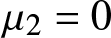 $\mu_2 = 0$ that bifurcates from the trigonometric limit
 $n_i = 0$. For example, when
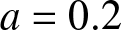 $a = 0.2$ in Figure 5, the level curve
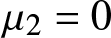 $\mu_2 = 0$ meets the trigonometric limit when
 $(n,m) \approx (0.878,0)$. Similarly, in Figure 6 with
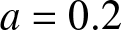 $a = 0.2$, the curve
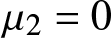 $\mu_2 = 0$ enters the domain from
 $(n_r,n_i) \approx (0.878,0)$. As
 $a$ varies, the level curves exhibit somewhat complex deformations. The level curve
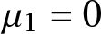 $\mu_1 = 0$ appears within the parameter window of consideration when
 $a = 2$. The boundary of the non-hyperbolic region is where
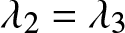 $\lambda_2 = \lambda_3$, so
 $\mu_2 = \mu_3 = 0$ there.
Convexity of the Whitham modulation equations for  $(\alpha,\beta) = (0,1)$ (case I), cubic interaction force with complex conjugate roots
 $w_{3,4}$,
 $\tilde{\mathbf{A}} = (n_r,n_i,a,\overline{v}=0) \in \tilde{E}_a$: The system is strictly hyperbolic in the white region. Greyscale is
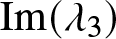 $\mathrm{Im}(\lambda_3)$ where the system is not hyperbolic. Periodic travelling waves do not exist in the inadmissible pink region. For each fixed amplitude
 $a$, the solid (dashed) curves correspond to the loss of genuine nonlinearity
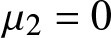 $\mu_2 = 0$ (
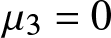 $\mu_3 = 0$). For
 $a = 2$, the dash-dotted curve corresponds to
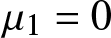 $\mu_1 = 0$.

Figure 6 Long description
The figure contains four contour plots illustrating the imaginary part of lambda 3 versus n r and n i for different values of parameter a. The x-axis is labeled n r, ranging from 0 to 1 and the y-axis is labeled n i, ranging from 0 to minus 1.5. Both axes are unitless. The plots show how the imaginary part of lambda 3 changes with these parameters. The color scale varies for each plot, indicating different ranges of the imaginary part of lambda 3. The solid and dashed curves represent boundaries of stability and loss of genuine nonlinearity, respectively. The masked peach regions indicate areas where periodic traveling waves do not exist. For a equals 0.2, the color scale ranges from 0 to 0.03. The solid curve encloses a region near n r equals 0.5 and n i equals 0. The dashed curves extend from n r equals 0 to n r equals 1, showing a loss of nonlinearity. For a equals 0.5, the color scale ranges from 0 to 0.08. The solid curve is positioned higher on the n i axis compared to the previous plot, indicating a shift in stability. For a equals 1, the color scale ranges from 0 to 0.1. The solid curve encloses a larger area and the dashed curves show a more pronounced downward slope, indicating changes in stability boundaries. For a equals 2, the color scale ranges from 0 to 0.15. The solid curve encloses the largest area and the dashed curves are positioned lower on the n i axis, indicating further changes in stability. The plots collectively show how increasing a affects the stability and nonlinearity regions, with the imaginary part of lambda 3 increasing in magnitude and the stability regions expanding.
4.5. Cubic nonlinearity with
$(\alpha,\beta) = (0,-1)$

Next, we discuss the case of cubic  $f(w)$ with
 $(\alpha,\beta)=(0,-1)$, which corresponds to case II in Section 3.2 after an appropriate rescaling discussed in Section 2.1. In this setting, we have
 \begin{equation*}
\begin{split}
\mathcal{W} &= \frac{1}{2\pi} \sqrt{\frac{6}{c^2}} \oint \sqrt{G_4(w)}\, \mathrm{d} w = \frac{1}{\pi} \sqrt{\frac{6}{c^2}} \int_{w_2}^{w_3} \sqrt{(w-w_1)(w-w_2)(w_3-w)(w_4-w)}\, \mathrm{d} w, \\
\overline{w^2} &= \frac{1}{2\pi} \sqrt{\frac{\omega^2}{6}} \oint \dfrac{w^2}{\sqrt{G_4(w)}}\, \mathrm{d} w
=\frac{1}{\pi} \sqrt{\frac{\omega^2}{6}} \int_{w_2}^{w_3} \dfrac{w^2\,\mathrm{d} w}{\sqrt{(w-w_1)(w-w_2)(w_3-w)(w_4-w)}}.
\end{split}
\end{equation*}
Recall that in this case, there are two families of periodic solutions related by symmetry (3.33) with  $\alpha=0$,
 $\beta=-1$ and that differ by a
 $\pi$ phase shift, so it suffices to consider one of them given by (3.41). We have
 \begin{equation*}
\begin{split}
&w_1 + w_2 + w_3 + w_4 = 0,\\
& A = -\frac{1}{2}(w_1w_2w_3 + w_1 w_2 w_4+w_1 w_3 w_4+w_2 w_3
w_4),\\
&c^2 = 1 + \frac{1}{2} ( w_1 w_2 + w_1 w_3 + w_1 w_4 + w_2 w_3 +
w_2 w_4 + w_3 w_4 ),\\
&k = \frac{\pi}{K(m)} \sqrt{\frac{3}{2c^2}(w_4-w_2)(w_3-w_1)}, \quad \omega=ck,\\
&m = \frac{(w_4-w_1)(w_3-w_2)}{(w_4-w_2)(w_3-w_1)},
\end{split}
\end{equation*}
where we used (3.7), (3.8), (3.11), (3.41) and (3.43), and obtain [Reference Byrd and Friedman4]
 \begin{equation}
\begin{split}
\mathcal{W}&=\dfrac{(w_3 - w_2)^2 (w_4-w_2)^{1/2} (w_2 -w_1)^2}{4|c| \sqrt{6}\pi
n^3 (1 - n)^2 (m-n)^2 (w_3-w_1)^{3/2}} \bigg\{n \bigg(3 n^4 + 3 m^2 - 4 n^3 (1 + m)\\
&- 4 n m (1 + m) + 2 n^2 (2 + m + 2 m^2)\bigg) E(m) \\
&+(m-n) \bigg(3 n^4 - 4 n^2 (m-1) - 3 m^2 +
6 n m^2 - 2 n^3 (2 + m)\bigg) K(m) \\
&+ 3 (m-n^2) (-2 n + n^2 + m) (n^2 + m -
2 n m) \Pi(n, m)\bigg\}
\end{split}
\end{equation}
and
 \begin{equation}
\begin{split}
\overline{w^2}&=\dfrac{\sqrt{2}w_1^2|\omega|}{\sqrt{3}\pi \sqrt{(w_3 - w_1) (w_4 - w_2)}}\bigg\{K(m) + 2\left(\dfrac{w_2}{w_1}-1\right)\Pi(n,m)\\
&+ \dfrac{(w_2 -w_1)^2}{2 (n-1) (m-n) w_1^2} \bigg(n E(m) + (m-n) K(m) \\
&- \bigg(n^2 + 3 m -
2 n (1 + m)\bigg) \Pi(n, m)\bigg)\bigg\},
\end{split}
\end{equation}
where we recall that  $m$ and
 $n$ are given in (3.41) and satisfy (3.42).
4.5.1. Solitary-wave limit
In the limit  $w_3 \to w_4$ (
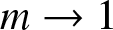 $m \to 1$), the solutions approach the two-parameter family (3.45) of solitary waves with amplitude
 $a=w_4-w_2$, background
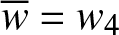 $\overline{w}=w_4$ and velocity (3.46). In this limit, we obtain
 \begin{equation}
\begin{split}
\lim_{w_3 \to w_4}\dfrac{c}{12}\mathcal{W}&=\dfrac{\text{sgn}(c)}{\pi\sqrt{6}}\bigg\{\dfrac{1}{6}\sqrt{a(4\overline{w}-a)}(a^2 - 4 a \overline{w} + 6 \overline{w}^2)\\
&-(a -2 \overline{w})^2 \overline{w}\, \text{arctanh}\sqrt{\dfrac{a}{4\overline{w}-a}}\biggl\},\\
\lim_{w_3 \to w_4}c\dfrac{\overline{w^2}-\overline{w}^2}{k}&=\dfrac{c^2\text{sgn}(c)}{\pi\sqrt{6}} \bigg\{-\sqrt{a(4\overline{w}-a)}+4\overline{w}\, \text{arctanh}\sqrt{\dfrac{a}{4\overline{w}-a}}\bigg\},\\
\lim_{w_3 \to w_4}\overline{w^2} &= \overline{w}^2, \quad \lim_{w_3 \to w_4}c^2=1-3\overline{w}^2+\dfrac{1}{2}a(4\overline{w}-a),
\end{split}
\end{equation}
where we recall that  $0 \lt a \lt 2\overline{w}$ by (3.47) with
 $\alpha = 0$. The Whitham modulation equations (4.7) with
 $f(w)=w-w^3$ therefore become
 \begin{equation}
\begin{split}
\overline{w}_T-\overline{v}_X&=0,\\
\overline{v}_T-(1-3\overline{w}^2)\overline{w}_X&=0,\\
a_T+c\,a_X+c\,\dfrac{g(a,\overline{w})}{d(a,\overline{w})}\overline{w}_X+\dfrac{h(a,\overline{w})}{d(a,\overline{w})}\overline{v}_X&=0,
\end{split}
\end{equation}
where
 \begin{equation}
\begin{split}
g(a,\overline{w})&=\sqrt{a(4\overline{w}-a)}(-2 + 4 a^2 - 19 a \overline{w} + 24 \overline{w}^2)\\
&+2 \bigg(-2 + (a - 6 \overline{w}) (a - 4 \overline{w})\bigg) (a - 2 \overline{w})\,\text{arctanh}\sqrt{\dfrac{a}{4 \overline{w}-a}},\\
h(a,\overline{w})&=\sqrt{a(4\overline{w}-a)} (-2 + 4 a^2 - 19 a \overline{w} + 24 \overline{w}^2)\\
&+\bigg(-4 + 3 (a - 4 \overline{w})^2\bigg) (a - 2 \overline{w})\, \text{arctanh}\sqrt{\dfrac{a}{4 \overline{w}-a}},\\
d(a,\overline{w})&=\sqrt{a(4\overline{w}-a)} (-1 + 2 a^2 - 8 a \overline{w} + 9 \overline{w}^2) -6 (a - 2 \overline{w})^2 \overline{w}\, \text{arctanh}\sqrt{\dfrac{a}{4 \overline{w}-a}}.
\end{split}
\end{equation}
The ordered characteristic velocities (for the fast-wave family with  $c \gt 0$) are
 \begin{equation}
\lambda_1 = -\sqrt{1-3\overline{w}^2}, \quad \lambda_2 = \sqrt{1-3\overline{w}^2}, \quad
\lambda_3 = c = \sqrt{1-3\overline{w}^2+\dfrac{1}{2}a(4\overline{w}-a)} .
\end{equation}
Note that the existence conditions (3.47) for  $(\alpha,\beta)=(0,-1)$ amount to satisfying one of the following inequality pairs
 \begin{equation}
\mathrm{either} \quad 0 \lt a \lt 2\overline{w} \quad \mathrm{and} \quad 0 \lt \overline{w}
\le \frac{1}{\sqrt{3}},
\end{equation}
 \begin{equation}
\mathrm{or} \quad 2\overline{w} - \sqrt{2(1-\overline{w}^2)} \lt a \lt 2\overline{w} \quad
\mathrm{and} \quad \frac{1}{\sqrt{3}} \lt \overline{w} \lt 1 .
\end{equation}
4.5.2. Kink limit
The limit  $a \to 2\overline{w}$ corresponds to the supersonic kink solution (3.48). To obtain its modulation, it is tempting to send
 $a \to 2\overline{w}$ in eq. (4.23). But this results in a singularity. Instead, we return to the wave-action equation (4.7c) with the solitary-wave limiting density and flux in eq. (4.22). We denote the limit as
 $a \to 2\hat{w}$ in order to distinguish the kink
 $\hat{w}$ from the mean
 $\overline{w}$. An expansion of the density and flux results in
 \begin{equation*}
\begin{split}
\frac{c}{12} \mathcal{W} + c \frac{\overline{w^2}-\overline{w}^2}{k}
&= -\frac{2\mathrm{sgn}(c)}{\pi\sqrt{6}}f(\hat{w}) \log(2\hat{w}-a) +
\mathcal{O}(1) , \\
c^2 \frac{\overline{w^2}-\overline{w}^2}{k}
&= -\frac{2|c|}{\pi\sqrt{6}}f(\hat{w}) \log(2\hat{w}-a) + \mathcal{O}(1) ,
\end{split}
\end{equation*}
as 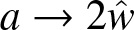 $a \to 2\hat{w}$ where
 $f(\hat{w}) = \hat{w}-\hat{w}^3$ is the interaction force and
 $c^2 = 1-\hat{w}^2$ is the squared kink velocity (3.49). Inserting this into the conservation of wave action (4.7c), we obtain the expansion
 \begin{equation*}
\frac{f(\hat{w})}{2\hat{w}-a}\left [ (2\hat{w}-a)_T + c (2\hat{w}-a)_X \right ] +
\log(2\hat{w}-a) \left [ f(\hat{w})_T + \left ( c f(\hat{w}) \right )_X \right ] +
\cdots = 0 .
\end{equation*}
Multiplying this expression by 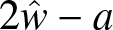 $2\hat{w}-a$ and equating each order to zero as
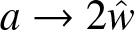 $a \to 2\hat{w}$, we obtain the kink conservation law
 \begin{equation*}
f(\hat{w})_T + \left [ c f(\hat{w}) \right]_X = 0, \quad f(\hat{w}) = \hat{w}-\hat{w}^3,
\quad c = \pm \sqrt{1-\hat{w}^2} .
\end{equation*}
This equation is distinct from the mean equations for  $(\overline{w},\overline{v})$ in (4.23) and admits the discontinuous travelling wave solution
 \begin{equation}
\hat{w}(X,T) = \pm 2w_0 \,\mathrm{sgn}(X-cT), \quad c^2 =
1-w_0^2, \quad 0 \lt w_0 \lt 1 ,
\end{equation}
whose velocity  $s = c$ results from the Rankine–Hugoniot jump condition
 $-s[f(\hat{w})] + [cf(\hat{w})] = 0$ where
 $[\cdot]$ is the difference between the state
 $\cdot$ to the right and left of the discontinuity. The weak solution (4.27) is the zero-dispersion limit of the kink solution (3.48) and thus is an admissible shock. Since the mean field propagates along characteristics with velocities
 $\lambda_j = \mp \sqrt{f'(\overline{w})} = \mp \sqrt{1-3\overline{w}^2}$, they are unchanged on either side of the shock (
 $f'(w_0) = f'(-w_0)$), i.e., the characteristics pass through the shock. It is because of this that the solution (4.27) can be interpreted as a non-classical, undercompressive shock [Reference El, Hoefer and Shearer17, Reference Herrmann and Rademacher23] and is an example of a superkink in the classification of steady transition fronts in mechanical systems [Reference Gorbushin, Vainchtein and Truskinovsky22].
4.5.3. Convexity
We start by considering the modulation system (4.23) with (4.24) for the solitary-wave family (3.45), with eigenvalues (4.25) and eigenvectors (4.19). The existence condition for this family is (4.26). In this case, we obtain
 \begin{equation*}
\mu_j=-\dfrac{3\overline{w}}{\lambda_j},\quad j=1,2, \quad \mu_3=\dfrac{2\overline{w}-a}{2\lambda_3}.
\end{equation*}
Thus, the system is strictly hyperbolic when  $0 \lt \overline{w} \lt 1/\sqrt{3}$ and genuinely nonlinear when
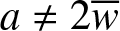 $a \neq 2\overline{w}$, which ensures that
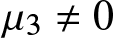 $ \mu_3 \neq 0$. Since a nonzero mean is required for the existence of a solitary wave,
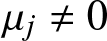 $\mu_j \ne 0$ for
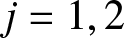 $j = 1,2$. We recall that the harmonic limit is strictly hyperbolic when
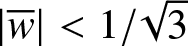 $|\overline{w}| \lt 1/\sqrt{3}$ and genuinely nonlinear when
 $\overline{w} \neq 0$ and
 $\omega \neq 0$.
To investigate the convexity of the full Whitham modulation system (4.7) with (4.20) and (4.21), we will present our results in terms of  $\mathbf{A}$ in (3.34). For several choices of the periodic travelling wave amplitude
 $a$, we plot the existence region and imaginary part of the second eigenvalue in Figure 7. Within the existence region, two islands nucleate where hyperbolicity is lost. The islands take up a larger percentage of the existence region as the wave amplitude is increased. To further understand these islands, we note that the depression solitary-wave limit with
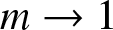 $m \to 1$ admits the following relation between the solitary-wave parameters
 $(a,\overline{w})$ and the parameter
 $n$ in (3.45)
 \begin{equation}
n = \frac{a}{4\overline{w}-a} , \quad 0 \lt a \lt 2 \overline{w} , \quad \overline{w} \gt 0 ,
\end{equation}
by  $a = w_4 - w_2$,
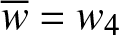 $\overline{w} = w_4$ and
 $w_1 + w_2 + 2w_4 = 0$. According to (4.25), we expect the nucleation of non-hyperbolic regions in the second characteristic family from
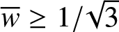 $\overline{w} \ge 1/\sqrt{3}$ in the solitary-wave limit. Indeed, the red segment in Fig. 7 along
 $m = 1$ corresponds to the values of
 $n$ in (4.28) satisfying the inequalities (4.26b) that yield
 $1/\sqrt{3} \lt \overline{w} \lt a/3 + \sqrt{2(6-a^2)}/6$.
Hyperbolicity of the Whitham modulation equations for  $(\alpha,\beta) = (0,-1)$ (case II). For each fixed amplitude
 $a$, the greyscale contour plot conveys the imaginary part of a characteristic velocity. Periodic waves do not exist in the inadmissible pink region. The solid (dashed) black curves correspond to the loss of genuine nonlinearity
 $\mu_1 = \mu_4 = 0$ (
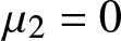 $\mu_2 = 0$). The red segment at
 $m = 1$ corresponds to the region of non-hyperbolicity of the solitary-wave limiting system (4.23).

Figure 7 Long description
A equals 0.15 A contour plot with a vertical color bar labeled Im lambda 2. No units are shown for m, n, or Im lambda 2. The horizontal axis is labeled m, with labeled ticks 0.2, 0.4, 0.6, 0.8, 1. The vertical axis is labeled n, with labeled ticks 0, 0.2, 0.4, 0.6, 0.8, 1. The color bar has labeled values 0, 0.05, 0.1, 0.15, 0.2, 0.25. A white region is enclosed by a solid black curve and dashed black curves. The solid curve passes from about m equals 0.2, n equals 0.1 to m equals 1, n equals 1. A dashed curve forms an upper boundary from about m equals 0.2, n equals 0.1 to m equals 1, n equals 1. A dashed curve forms a lower boundary close to n equals 0 from about m equals 0.2 to m equals 1. a equals 0.5 A contour plot with a vertical color bar labeled Im lambda 2. No units are shown for m, n, or Im lambda 2. The horizontal axis is labeled m, with labeled ticks 0.5, 0.6, 0.7, 0.8, 0.9, 1. The vertical axis has labeled ticks 0.2, 0.4, 0.6, 0.8, 1. The color bar has labeled values 0, 0.1, 0.2, 0.3, 0.4, 0.5. A white region is enclosed by a solid black curve and dashed black curves. The solid curve passes from about m equals 0.5, n equals 0.3 to m equals 1, n equals 1. A dashed curve forms an upper boundary from about m equals 0.5, n equals 0.3 to m equals 1, n equals 1. A dashed lower boundary runs from about m equals 0.5, n equals 0.3 down toward about n equals 0.2 around m equals 0.8 to 0.9, then continues toward m equals 1 near about n equals 0.25. Shading appears within the bounded region near m close to 1 and n about 0.2 to 0.3. a equals 1 A contour plot with a vertical color bar labeled Im lambda 2. No units are shown for m, n, or Im lambda 2. The horizontal axis is labeled m, with labeled ticks 0.8, 0.85, 0.9, 0.95, 1. The vertical axis is labeled n, with labeled ticks 0.4, 0.5, 0.6, 0.7, 0.8, 0.9, 1. The color bar has labeled values 0, 0.1, 0.2, 0.3, 0.4, 0.5, 0.6. A white region is enclosed by a solid black curve and dashed black curves. The solid curve passes from about m equals 0.8, n equals 0.55 to m equals 1, n equals 1. A dashed curve forms an upper boundary approaching m equals 1, n equals 1. A dashed lower boundary dips from about m equals 0.8, n equals 0.55 down toward about n equals 0.45 around m equals 0.95, then turns upward toward m equals 1. Shading occupies the bounded region for m close to 1 and n about 0.45 to 0.6. a equals 1.3 A contour plot with a vertical color bar labeled Im lambda 2. No units are shown for m, n, or Im lambda 2. The horizontal axis is labeled m, with labeled ticks 0.9, 0.92, 0.94, 0.96, 0.98, 1. The vertical axis has labeled ticks 0.5, 0.6, 0.7, 0.8, 0.9, 1. The color bar has labeled values 0, 0.2, 0.4, 0.6. A white region is enclosed by a solid black curve and dashed black curves. The solid curve passes from about m equals 0.9, n equals 0.68 to m equals 1, n equals 1. A dashed curve forms an upper boundary approaching m equals 1, n equals 1. A dashed lower boundary dips from about m equals 0.9, n equals 0.68 down toward about n equals 0.6 around m equals 0.96, then rises toward m equals 1. Shading fills much of the bounded region for m close to 1, spanning n about 0.6 up to near 1. Across the four plots, the shaded area associated with nonzero Im lambda 2 is concentrated at m close to 1 and expands to a wider n range as a increases from 0.15 to 1.3, while the color bar maximum increases from 0.25 to 0.6.
Figure 7 also depicts the level curves 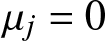 $\mu_j = 0$. The solid black curve corresponds to both
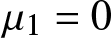 $\mu_1 = 0$ and
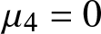 $\mu_4 = 0$. It bifurcates from the kink limit
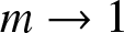 $m \to 1$,
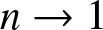 $n \to 1$. The dashed curves correspond to regions where
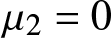 $\mu_2 = 0$. Necessarily, these surround the non-hyperbolic greyscale regions where
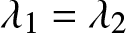 $\lambda_1 = \lambda_2$ because the coalescence of two characteristics (non-strict hyperbolicity) coincides with loss of genuine nonlinearity, so that
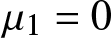 $\mu_1 = 0$ also there.
5. Stability of periodic travelling waves
The loss of hyperbolicity in the modulation equations discussed in Sections 4.3.2, 4.4.2 and 4.5.3 corresponds to modulational instability of the corresponding periodic travelling wave [Reference Whitham39]. To verify the onset of such an instability, we numerically compute the spectrum of the linearized operator for various parameter values and solve initial value problems with suitably perturbed periodic travelling wave initial data.
To obtain the corresponding eigenvalue problem, we first observe that (2.7) is equivalent to
 \begin{equation}
w_t=v_x, \qquad v_t=\left(1-\dfrac{1}{12}\partial_x^2\right)^{-1}(f(w))_x,
\end{equation}
where we used  $w_{tt}=v_{xt}$. Rewriting (5.1) in terms of
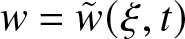 $w=\tilde{w}(\xi,t)$,
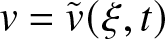 $v=\tilde{v}(\xi,t)$,
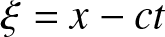 $\xi=x-ct$, we obtain
 \begin{equation*}
\tilde{w}_t=\tilde{v}_\xi+c\tilde{w}_\xi, \qquad \tilde{v}_t=\left(1-\dfrac{1}{12}\partial_\xi^2\right)^{-1}(f(w))_\xi+c\tilde{v}_\xi.
\end{equation*}
Seeking solutions of this system in the form
 \begin{equation*}
\left[\begin{array}{c} \tilde{w}\\\tilde{v}\end{array}\right]=\left[\begin{array}{c}W(\xi)\\V(\xi)\end{array}\right]+\varepsilon e^{\lambda t}
\boldsymbol{\phi}(\xi),
\end{equation*}
where  $W(\xi)$ and
 $V(\xi)$ are the strain and particle velocity for a periodic travelling wave with period
 $T_0$,
 \begin{equation*}
W(\xi+T_0)=W(\xi), \quad V(\xi+T_0)=V(\xi),
\end{equation*}
and keeping only terms of order  $\varepsilon$, we obtain the following eigenvalue problem for the linearized operator:
 \begin{equation}
\lambda \boldsymbol{\phi}=\left[\begin{array}{ll} c\partial_\xi & \;\;\partial_\xi\\
\left(1-\dfrac{1}{12}\partial_\xi^2\right)^{-1}\partial_\xi f'(W(\xi)) & \;\;c\partial_\xi\end{array}\right]\boldsymbol{\phi}.
\end{equation}
By Floquet theory applied to the  $T_0$-periodic linear operator in the right-hand side of (5.2), the eigenvalue
 $\lambda$ is in the spectrum if and only if there exists a nonzero eigenfunction
 $\boldsymbol{\phi}$ such that [Reference Chicone5]
 \begin{equation*}
\boldsymbol{\phi}(\xi+T_0)=e^{\frac{2\pi iq\xi}{T_0}}\boldsymbol{\phi}(\xi)
\end{equation*}
for some real  $q$. This implies [Reference Bronski, Hur and Wester2] that there exists
 $\boldsymbol{\psi}$ such that
 \begin{equation}
\boldsymbol{\phi}(\xi+T_0)=e^{\frac{2\pi i \tau \xi}{T_0}}\boldsymbol{\psi}(\xi), \quad \boldsymbol{\psi}(\xi+T_0)=\boldsymbol{\psi}(\xi),
\end{equation}
where  $\tau \in (-1/2,1/2]$ is the Floquet parameter. Thus, we have
 \begin{equation}
\boldsymbol{\psi}(\xi)=\sum_{q\in\mathbb{Z}}\hat{\boldsymbol{\psi}}_q \exp\dfrac{2\pi i q\xi}{T_0}\,
\end{equation}
where  $\hat{\boldsymbol{\psi}}_q$ are the Fourier coefficients of
 $\boldsymbol{\psi}$. Using (5.2) and (5.3), we obtain
 \begin{equation}
\begin{split}
&\lambda \boldsymbol{\psi}=\left[\begin{array}{ll} c\left(\frac{2\pi i\tau}{T_0}+\partial_\xi\right) & \;\;\frac{2\pi i\tau}{T_0}+\partial_\xi\\
M(\tau) f'(W(\xi)) & \;\;c\left(\frac{2\pi i\tau}{T_0}+\partial_\xi\right)\end{array}\right]\boldsymbol{\psi}, \\
&M(\tau)=\left(1-\dfrac{1}{12}\left(\frac{2\pi i\tau}{T_0}+\partial_\xi\right)^2\right)^{-1}\left(\frac{2\pi i\tau}{T_0}+\partial_\xi\right).
\end{split}
\end{equation}
To numerically compute the spectrum of the linear operator, we use the Floquet–Fourier–Hill method [Reference Deconinck and Kutz10]. Following the procedure in [Reference Bronski, Hur and Wester2], we restrict the values of  $q$ in (5.4) to
 $q=-N_q,\dots,N_q$ and use Fourier collocation to project (5.5) to a subspace of
 $L^2(-T_0/2,T_0/2) \times L^2(-T_0/2,T_0/2)$. This reduces the problem to finding eigenvalues of a
 $(4N_q+1)\times(4N_q+1)$ matrix
 $\mathbf{L}(\tau)$, which is computed by taking sums and products of diagonal and Toeplitz matrices that represent differential operators and multiplications by periodic functions in (5.5), respectively. Computing these eigenvalues for each value of
 $\tau$ in the
 $N_\tau$-point discretization of
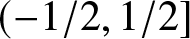 $(-1/2,1/2]$, we obtain the numerical approximation of the spectrum. In what follows, we use
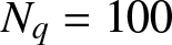 $N_q=100$ and
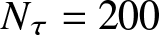 $N_\tau=200$. Since
 $f'(W(\xi))=1+2\alpha W(\xi)+3\beta W^2(\xi)$, the procedure requires computing the Fourier coefficients of
 $W(\xi)$ in the quadratic nonlinearity case
 $(\alpha,\beta)=(1,0)$ and
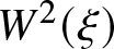 $W^2(\xi)$ in the case of cubic nonlinearity, where
 $(\alpha,\beta)=(0,\pm 1)$. In the case of quadratic nonlinearity, the coefficients can be found analytically using the Fourier expansion for
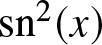 $\text{sn}^2(x)$ [Reference Kiper28]:
 \begin{equation*}
W(\xi)=\sum_{q\in\mathbb{Z}} \hat{W}_q e^\frac{2\pi iq\xi}{T_0}, \quad
\hat{W}_q=\begin{cases} (w_3-w_2)\frac{\pi^2q\kappa^q}{m K^2(m)(1-\kappa^{2q})}, & q\neq 0 \\
w_3-(w_3-w_2)\frac{K(m)-E(m)}{mK(m)}, & q=0
\end{cases}, \quad \kappa=\exp\dfrac{\pi K(1-m)}{K(m)}.
\end{equation*}
For the cubic nonlinearity cases, the Fourier coefficients were computed using numerical integration in Mathematica. To speed up the computations, we took advantage of the fact that these coefficients quickly decay as  $|q|$ tends to infinity so we restricted the computed coefficients to
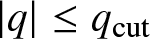 $|q| \leq q_\text{cut}$, setting the rest to zero. In most cases,
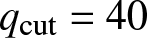 $q_\text{cut}=40$ was sufficient.
We begin by examining the spectra in the case of quadratic nonlinearity (Case III) with  $(\alpha,\beta) = (1,0)$. The top panel in Fig. 8 zooms in around the top of the grey region in Fig. 3(a), where the Whitham modulation system loses hyperbolicity. As we enter this region, we expect to see the onset of modulational instability of periodic travelling waves. To check this, we compute the linear spectrum for periodic travelling waves at the parameter values
 $m$ and
 $a$ corresponding to points
 $A$ and
 $B$, located just outside and just inside the grey region, respectively. The corresponding spectra are shown in the two middle panels of Figure 8. Eigenvalues away from the imaginary axis correspond to instabilities. One can see that both solutions exhibit short-wavelength instabilities (
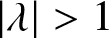 $|\lambda| \gt 1$,
 $\text{Re}(\lambda) \neq 0$), including superharmonic instabilities, studied in detail in [Reference Bronski, Hur and Wester2], which are associated with the spectrum tending to infinity along vertical asymptotes. Note, however, the spectrum at
 $A$ does not exhibit modulational instability (long wavelength,
 $\lambda \sim 0$ with nonzero real part), while the characteristic cross pattern of the spectrum near the origin associated with modulational instability is clearly seen at
 $B$, the point just inside the grey region. A similar emergence of modulational instability can be seen as we transition from point
 $C$ just outside the grey region to the point
 $D$ just inside it, as illustrated by the bottom panels in Fig. 8.
Top panel: Fig. 3(a) zoomed in around the tip of the grey region where the Whitham system loses hyperbolicity in the case of quadratic nonlinearity ( $\alpha=1$,
 $\beta=0$). Middle and bottom panels: spectra of the linear operator at the parameter values marked by points
 $A$,
 $B$,
 $C$ and
 $D$ in the top panel.

Figure 8 Long description
A) The plot shows Im(lambda2) as a filled contour map over m and a. Units are not shown for m, a, or Im(lambda2). The x-axis is labeled m and ranges from 0.83 to 0.90. The y-axis is labeled a and ranges from 2.2 to 2.8. A vertical scale bar is labeled Im(lambda2) and ranges from 0 to 0.7. Four labeled points appear: A near m equals 0.886 and a equals 2.26, B near m equals 0.886 and a equals 2.27, C near m equals 0.832 and a equals 2.69 and D near m equals 0.834 and a equals 2.69. B) The plot title reads A: m equals 0.886, a equals 2.26. The plot shows a spectrum in the complex plane with Re(lambda) on the horizontal axis and Im(lambda) on the vertical axis. Units are not shown for Re(lambda) or Im(lambda). Re(lambda) ranges from minus 1.5 to 1.5. Im(lambda) ranges from minus 10 to 10. The plotted spectrum consists of two solid outer branches and a central feature at Re(lambda) equals 0. The outer upper branch is near Im(lambda) equals 10 at Re(lambda) near minus 1.5 and near plus 1.5 and it dips to about Im(lambda) equals 5 near Re(lambda) equals 0. The outer lower branch mirrors this, reaching near Im(lambda) equals minus 10 at Re(lambda) near minus 1.5 and near plus 1.5 and rising to about Im(lambda) equals minus 5 near Re(lambda) equals 0. At Re(lambda) equals 0, a thin vertical segment runs from about Im(lambda) equals minus 5 to about Im(lambda) equals plus 5. Two small closed loops lie on this vertical segment, one centered near Im(lambda) about plus 2 and one centered near Im(lambda) about minus 2. C) The plot title reads B: m equals 0.886, a equals 2.27. The plot shows Re(lambda) versus Im(lambda) with the same axis labels and ranges as the previous spectrum plot: Re(lambda) from minus 1.5 to 1.5 and Im(lambda) from minus 10 to 10, with units not shown. The outer upper and lower solid branches have the same overall placement as in the A spectrum plot, with the upper branch dipping to about Im(lambda) equals 5 near Re(lambda) equals 0 and the lower branch rising to about Im(lambda) equals minus 5 near Re(lambda) equals 0. The central feature at Re(lambda) equals 0 again spans about Im(lambda) equals minus 5 to about Im(lambda) equals plus 5, but the closed loop around the origin is larger than in the A spectrum plot and forms a wider, pinched shape around Im(lambda) equals 0. D) The plot title reads C: m equals 0.832, a equals 2.69. The plot shows Re(lambda) versus Im(lambda), with Re(lambda) from minus 1.5 to 1.5 and Im(lambda) from minus 10 to 10 and units not shown. Two large solid branches form a symmetric crossing at the center, meeting near Re(lambda) equals 0 and Im(lambda) equals 0. Above the crossing, the branches widen outward and form broad lobes around Im(lambda) about plus 5, then narrow again toward Im(lambda) near plus 10. Below the crossing, the branches mirror this around Im(lambda) about minus 5 and narrow toward Im(lambda) near minus 10. Short dotted segments appear near Im(lambda) between about plus 6 and plus 8 and also between about minus 6 and minus 8, aligned near Re(lambda) values close to 0. E) The plot title reads D: m equals 0.834, a equals 2.69. The plot shows Re(lambda) versus Im(lambda), with Re(lambda) from minus 1.5 to 1.5 and Im(lambda) from minus 10 to 10 and units not shown. The solid branches again cross near Re(lambda) equals 0 and Im(lambda) equals 0 and form broad lobes around Im(lambda) about plus 5 and about minus 5, narrowing toward Im(lambda) near plus 10 and near minus 10. Dotted segments again appear near Im(lambda) between about plus 6 and plus 8 and between about minus 6 and minus 8, near Re(lambda) close to 0. Across the spectra plots, the A and B cases share the same m value (0.886) with a changing from 2.26 to 2.27 and the central closed loop feature around Re(lambda) equals 0 is larger in the B case than in the A case. The C and D cases share the same a value (2.69) with m changing from 0.832 to 0.834 and the overall crossing and lobe shapes remain similar between these two spectra. Solid and dotted curve segments are both present in the C and D spectra plots, with no legend explaining the difference.
To see the dynamical consequences of modulational instability, we perturb the periodic travelling wave at  $m=0.886$,
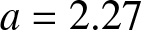 $a=2.27$ (point
 $B$ in the top panel of Fig. 8), the strain component of which is shown in Fig. 9(a), by adding the unstable mode associated with the eigenvalue
 $\lambda=0.0019+0.0883i$ (shown in Fig. 9(b)), with the amplitude of perturbation
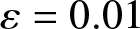 $\varepsilon=0.01$. The strain snapshot at
 $t=8$ is shown in panel (c) of Fig. 9, with panels (d) and (e) zooming in on the top and left side of the strain profile, respectively. One can see that the strain profile clearly develops modulational instability of the same wavelength as the perturbation mode. Note, however, that in addition to this, a short-wavelength instability develops as well, as can be seen in panel (e), in agreement with the spectrum shown in the middle right panel of Figure 8 (point
 $B$). This instability is numerically found to eventually lead to the blowup of the solution.
(a) The strain component  $W(\xi)$ of the periodic travelling wave solution at
 $m=0.886$,
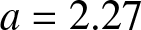 $a=2.27$. (b) Real part of the first component
 $\phi_1$ of the eigenfunction associated with the eigenvalue
 $\lambda=0.0019+0.0883i$. (c) Strain profile at
 $t=8$ in the dynamical simulation initiated by the travelling wave perturbed by the unstable mode, with perturbation amplitude
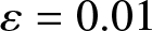 $\varepsilon=0.01$. (d) Panel (c) zoomed in around the top part. (e) Panel (c) zoomed in around the left part.

Figure 9 Long description
The image A showing a line graph with the vertical axis labeled w and the horizontal axis labeled xi. The horizontal axis runs from 0 to 90 with labeled ticks at 0, 10, 20, 30, 40, 50, 60, 70, 80, 90. The vertical axis runs from minus 1 to 1.5 with labeled ticks at minus 1, minus 0.5, 0, 0.5, 1, 1.5. A single oscillatory curve spans the full x-range with many closely spaced cycles. Peaks reach about 1.4 to 1.5 and troughs reach about minus 0.9 to minus 1. The image B showing a line graph with the vertical axis labeled Re of phi 1 and the horizontal axis labeled xi. The horizontal axis runs from 0 to 90 with labeled ticks at 0, 10, 20, 30, 40, 50, 60, 70, 80, 90. The vertical axis runs from minus 1.5 to 1.5 with labeled ticks at minus 1.5, minus 1, minus 0.5, 0, 0.5, 1, 1.5. A single oscillatory curve has a varying envelope. The oscillations are small near xi close to 0, grow to a large envelope around xi about 20 to 30 with peaks near 1.2 and troughs near minus 1.2, reduce to a narrow waist around xi about 45 where the amplitude is near 0, then grow again around xi about 65 to 75 with peaks near 1.2 and troughs near minus 1.2 and reduce again toward xi near 90. The image C showing a line graph with the vertical axis labeled w and the horizontal axis labeled x. The horizontal axis runs from 0 to 90 with labeled ticks at 0, 10, 20, 30, 40, 50, 60, 70, 80, 90. The vertical axis runs from minus 1 to 1.5 with labeled ticks at minus 1, minus 0.5, 0, 0.5, 1, 1.5. A single oscillatory curve spans the full x-range with many closely spaced cycles. The upper peaks remain near 1.4 to 1.5 across the range. The lower part shows localized deeper dips below about minus 0.5 around x about 15 to 30 and again around x about 60 to 80, with troughs approaching about minus 1. The image D showing a line graph with the vertical axis labeled w and the horizontal axis labeled x. The horizontal axis shows labeled ticks at 10, 20, 30, 40, 50, 60, 70, 80. The vertical axis shows labeled ticks at 1.25, 1.3, 1.35, 1.4, 1.45. A dense oscillatory trace is shown within a narrow vertical band. The top envelope stays near about 1.41 to 1.42 with slight variation across x and the lower parts of the oscillations extend down to near about 1.25. The image E showing a line graph with the vertical axis labeled w and the horizontal axis labeled x. The horizontal axis runs from 0 to 30 with labeled ticks at 0, 5, 10, 15, 20, 25, 30. The vertical axis runs from minus 1 to 1.5 with labeled ticks at minus 1, minus 0.5, 0, 0.5, 1, 1.5. A single oscillatory curve shows repeated cycles across the full range. Peaks reach near 1.4 to 1.5 and troughs reach near minus 0.9 to minus 1. Several small downward notches appear along the lower part of the curve between about x 10 and x 30.
To check the onset of modulational instability in the case  $(\alpha,\beta) = (0,-1)$ (Case II), we consider the parameter values at points
 $A$-
 $F$ in Fig. 10, which zooms in on the area in Fig. 7(d) (for periodic travelling waves of amplitude
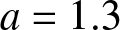 $a=1.3$) near the tips of the grey regions where the Whitham system loses hyperbolicity. The corresponding spectra are shown in Fig. 11. One can see that the modulational instability develops as we transition from point
 $A$ outside the lower grey region to point
 $B$ inside it (top panels). Point
 $C$ is still inside the region, and the corresponding spectrum (left middle panel of Figure 11) shows modulational instability. This instability disappears at point
 $D$ (right middle panel), which is outside the grey region. The spectrum at point
 $E$, which is still in the domain of strict hyperbolicity (see Figure 10), is shown in the left lower panel of Fig. 11. One can see the modulational instability developing again at point
 $E$ (right lower panel), which is just inside the top grey region in Figure 10. Note that in all cases there are short-wavelength instabilities.
Fig. 7(d) (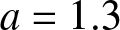 $a=1.3$) zoomed in near the tips of the grey regions where the Whitham system loses hyperbolicity in the case of cubic nonlinearity with
 $(\alpha,\beta) = (0,-1)$. Spectra shown in Fig. 11 were computed at the parameter values marked by the points
 $A$-
 $F$.

Figure 10 Long description
The x-axis is labeled m, with units not shown. The labeled range is 0.954 to 0.966, with tick labels 0.954, 0.956, 0.958, 0.96, 0.962, 0.964 and 0.966. The y-axis is labeled n, with units not shown. The labeled range is 0.55 to 0.9, with tick labels 0.55, 0.6, 0.65, 0.7, 0.75, 0.8, 0.85 and 0.9. A vertical color scale is labeled Im lambda 2, with labeled values 0, 0.1, 0.2, 0.3, 0.4, 0.6 and 0.7. The plot background contains a filled contour field that varies with m and n. Two shaded regions are visible within the contour field. One region spans approximately n equals 0.56 to n equals 0.66 across the shown m range. Another region spans approximately n equals 0.89 to n equals 0.91 across the shown m range. Two overlaid lines cross the contour field. One solid line increases with m, passing at about n equals 0.79 near m equals 0.954 and about n equals 0.82 near m equals 0.966. One dashed line decreases slightly with m, passing at about n equals 0.57 near m equals 0.954 and about n equals 0.56 near m equals 0.966. Six open circular markers are plotted near m equals 0.96 and labeled A, B, C, D, E and F. Their approximate coordinates are: A at m equals 0.96 and n equals 0.58; B at m equals 0.96 and n equals 0.59; C at m equals 0.96 and n equals 0.64; D at m equals 0.96 and n equals 0.65; E at m equals 0.96 and n equals 0.88; F at m equals 0.96 and n equals 0.89. Points A, B, C and D fall within the n range of the lower shaded region. Point F falls within the n range of the upper shaded region. Point E is just below the n range of the upper shaded region. No definitions for m, n, or Im lambda 2 are shown in the figure and no legend text is provided for the solid line, dashed line, or shaded regions.
Spectra of the linear operator at the parameter values marked by points  $A$-
 $F$ in Fig. 10.

Figure 11 Long description
A) Title: A: m equals 0.96, n equals 0.58. Plot type: complex-plane line plot of Re(lambda) versus Im(lambda). Units: no units shown. The horizontal axis is labeled Re(lambda), ranging from minus 2 to 2. The vertical axis is labeled Im(lambda), ranging from minus 10 to 10. A symmetric solid curve forms two wide lobes centered near Im(lambda) about plus 4 and minus 4, narrowing toward Re(lambda) equals 0 near Im(lambda) equals 0. Two short solid vertical segments lie on Re(lambda) equals 0, one between Im(lambda) about 5 and 6 and one between Im(lambda) about minus 6 and minus 5. Dotted curve segments appear near Im(lambda) about plus 5 and minus 5 for Re(lambda) less than 0 and for Re(lambda) greater than 0. Dotted segments are shown; meaning not specified. B) Title: B: m equals 0.96, n equals 0.59. Plot type: complex-plane line plot of Re(lambda) versus Im(lambda). Units: no units shown. The horizontal axis is labeled Re(lambda), ranging from minus 2 to 2. The vertical axis is labeled Im(lambda), ranging from minus 10 to 10. A symmetric solid curve forms upper and lower lobes that cross at Re(lambda) equals 0 and Im(lambda) equals 0, creating an X-shaped intersection at the center. Two short solid vertical segments lie on Re(lambda) equals 0, one near Im(lambda) about 5 to 6 and one near Im(lambda) about minus 6 to minus 5. C) Title: C: m equals 0.96, n equals 0.64. Plot type: complex-plane line plot of Re(lambda) versus Im(lambda). Units: no units shown. The horizontal axis is labeled Re(lambda), ranging from minus 1 to 1. The vertical axis is labeled Im(lambda), ranging from minus 10 to 10. A symmetric solid curve forms an X-shaped crossing at Re(lambda) equals 0 and Im(lambda) equals 0, with branches opening outward toward Re(lambda) near minus 1 and plus 1 as Im(lambda) approaches plus 10 and minus 10. Two small isolated points lie on Re(lambda) equals 0, one near Im(lambda) about plus 4 and one near Im(lambda) about minus 4. D) Title: D: m equals 0.96, n equals 0.65. Plot type: complex-plane line plot of Re(lambda) versus Im(lambda). Units: no units shown. The horizontal axis is labeled Re(lambda), ranging from minus 1 to 1. The vertical axis is labeled Im(lambda), ranging from minus 10 to 10. A symmetric solid curve has a narrow central solid vertical connection on Re(lambda) equals 0 from Im(lambda) about minus 2 to plus 2, with upper and lower branches that widen outward as Im(lambda) increases in magnitude. Two short solid vertical segments lie on Re(lambda) equals 0, one near Im(lambda) about plus 3 to 4 and one near Im(lambda) about minus 4 to minus 3. E) Title: E: m equals 0.96, n equals 0.88. Plot type: complex-plane line plot of Re(lambda) versus Im(lambda). Units: no units shown. The horizontal axis is labeled Re(lambda), ranging from minus 1 to 1. The vertical axis is labeled Im(lambda), ranging from minus 10 to 10. A symmetric solid curve forms two separated outer branches, one in the upper half and one in the lower half, leaving a central gap around Im(lambda) near 0. A long solid vertical line segment lies on Re(lambda) equals 0 from Im(lambda) about minus 4 to plus 4. Short dotted horizontal segments appear near Im(lambda) about plus 3 and minus 3 for Re(lambda) less than 0 and for Re(lambda) greater than 0. Dotted segments are shown; meaning not specified. F) Title: F: m equals 0.96, n equals 0.89. Plot type: complex-plane line plot of Re(lambda) versus Im(lambda). Units: no units shown. The horizontal axis is labeled Re(lambda), ranging from minus 1 to 1. The vertical axis is labeled Im(lambda), ranging from minus 10 to 10. A symmetric solid curve forms an X-shaped crossing at Re(lambda) equals 0 and Im(lambda) equals 0, with branches opening outward toward Re(lambda) near minus 1 and plus 1 as Im(lambda) approaches plus 10 and minus 10. Two small isolated points lie on Re(lambda) equals 0, one near Im(lambda) about plus 4 and one near Im(lambda) about minus 4. Across A to F, m remains 0.96 while n increases from 0.58 to 0.89. The plotted spectra alternate between a central X-shaped crossing at Re(lambda) equals 0 and Im(lambda) equals 0 (B, C, F) and shapes with a central vertical connection or gap on Re(lambda) equals 0 (A, D, E).
When the spectrum exhibits modulational instability, one can see a characteristic cross structure near the origin. The slopes of this structure can be estimated using the complex-valued Whitham characteristic velocities  $\sigma$ and
 $\bar{\sigma}$ that lead to the instability. Indeed, for small wavenumber
 $k$ we have
 $\text{Re}(\lambda) \approx k\text{Im}(\sigma)$ and
 $\text{Im}(\lambda) \approx k(\text{Re}(\sigma)-c)$, so that the slope
 $\text{Im}(\lambda)/\text{Re}(\lambda) \approx
(\text{Re}(\sigma)-c)/\text{Im}(\sigma)$, and the same is true for
 $\bar{\sigma}$. To illustrate this, we show in Figure 12 the red lines with the corresponding slopes superimposed with the spectra at the parameter values marked by points
 $B$,
 $C$ and
 $F$ in Fig. 10 zoomed in around the origin.
Spectra of the linear operator at the parameter values marked by points  $B$,
 $C$ and
 $F$ in Fig. 10 zoomed in around the origin, shown together with red straight lines obtained from the analysis of the Whitham system. See the text for details.

Finally, we consider Case I with  $(\alpha,\beta)=(0,1)$. Recall that in the case when all roots are real, no loss of hyperbolicity is observed, and thus all periodic travelling waves are expected to be modulationally stable (cf. Fig. 5). However, other instability modes are still present, as illustrated in Figure 13, where we use the transformation (3.35) to the parameter values (3.34). In the case when
 $w_{3,4}$ are complex, we found that the Whitham modulation equations are no longer hyperbolic in certain parameter regimes as shown in Fig. 6. We use the transformation (3.39) to present the results in terms of (3.38) and recall that the existence region for the periodic travelling waves is given by (3.40). As shown in the top panel of Figure 14 (see also Figure 6 with
 $a = 1$), in this case there is a grey region associated with the loss of hyperbolicity and onset of modulational instability. This instability mode is evident in the spectra at points
 $A$ and
 $C$ just inside this region (left middle and bottom panels) and disappears in the spectra at points
 $B$ and
 $D$ just outside the grey region (right middle and bottom panels). However, the spectra at
 $B$ and
 $D$ feature short-wavelength instabilities.
Spectra of the linear operator at different values of parameter  $m$ for Case I with
 $(\alpha,\beta)=(0,1)$ and real roots. Here
 $a=1$ and
 $n=0.5$.

Figure 13 Long description
The image A showing the title m equals 0.1. The horizontal axis label is Re left parenthesis lambda right parenthesis. The horizontal axis tick labels are negative 0.1, negative 0.05, 0, 0.05, 0.1. The vertical axis label is Im left parenthesis lambda right parenthesis. The vertical axis tick labels are negative 8, negative 4, 0, 4, 8. A vertical line is drawn at Re left parenthesis lambda right parenthesis equals 0. Two horizontal bands of plotted points appear near Im left parenthesis lambda right parenthesis around positive 7 to 8 and around negative 7 to 8, extending across Re left parenthesis lambda right parenthesis values on both sides of 0. The image B showing the title m equals 0.5. The horizontal axis label is Re left parenthesis lambda right parenthesis. The horizontal axis tick labels are negative 0.04, 0, 0.04. The vertical axis label is Im left parenthesis lambda right parenthesis. The vertical axis tick labels are negative 10, 0, 10. A vertical line is drawn at Re left parenthesis lambda right parenthesis equals 0. Plotted points form several horizontal groupings: one grouping near Im left parenthesis lambda right parenthesis around positive 12 to 13 close to Re left parenthesis lambda right parenthesis near 0, one grouping near Im left parenthesis lambda right parenthesis around negative 12 to 13 close to Re left parenthesis lambda right parenthesis near 0 and additional sparse points around Im left parenthesis lambda right parenthesis near positive 3 to 4 and near negative 3 to 4 spread across Re left parenthesis lambda right parenthesis values on both sides of 0. The image C showing the title m equals 0.9. The horizontal axis label is Re left parenthesis lambda right parenthesis. The horizontal axis tick labels are negative 0.02, 0, 0.02. The vertical axis label is Im left parenthesis lambda right parenthesis. The vertical axis tick labels are negative 10, negative 5, 0, 5, 10. A vertical line is drawn at Re left parenthesis lambda right parenthesis equals 0. Plotted points form multiple horizontal groupings: a grouping near Im left parenthesis lambda right parenthesis around positive 10 close to Re left parenthesis lambda right parenthesis near 0, a grouping near Im left parenthesis lambda right parenthesis around negative 10 close to Re left parenthesis lambda right parenthesis near 0 and several additional groupings between about negative 5 and positive 5 spread across Re left parenthesis lambda right parenthesis values on both sides of 0.
Top panel: upper left part of  $a=1$ panel in Fig. 6 for Case I with
 $(\alpha,\beta)=(0,1)$, real
 $w_{1,2}$ and complex
 $w_{3,4}$. Bottom panels: spectra of the linear operator at the parameter values marked by points
 $A$-
 $D$ in the top panel.

Figure 14 Long description
The image A showing a scientific plot that maps Im(lambda3) over the complex parameter eta and marks four eta values A, B, C and D used for the spectra in the other images. Axes show real and imaginary parts, with no physical units shown. The image A showing a shaded parameter map. The horizontal axis label is Re(eta) with tick labels 0, 0.1, 0.2, 0.3, 0.4 and 0.5. The vertical axis label is Im(eta) with tick labels minus 0.1, minus 0.2, minus 0.3, minus 0.4, minus 0.5, minus 0.6, minus 0.7, minus 0.8 and minus 0.9. A color scale at the right is labeled Im(lambda3) with tick labels 0.02, 0.04, 0.06, 0.08, 0.1, 0.12 and 0.14. Four labeled points appear: A and B at Im(eta) about minus 0.75 with Re(eta) about 0.25 and 0.27 and C and D at Im(eta) about minus 0.95 with Re(eta) about 0.4 and 0.42. The image B showing a complex-plane spectrum plot titled A: eta equals 0.25 minus 0.75i. The horizontal axis label is Re(lambda) with a multiplier label times 10 superscript minus 3 and tick labels minus 5, minus 4, minus 3, minus 2, minus 1, 0, 1, 2, 3, 4 and 5. The vertical axis label is Im(lambda) with tick labels minus 0.2, minus 0.1, 0, 0.1 and 0.2. A vertical dotted line is drawn at Re(lambda) equals 0. Blue points form two symmetric arc-shaped point sets about Im(lambda) equals 0, spanning roughly Re(lambda) from about minus 4.5 to plus 4.5 on the times 10 superscript minus 3 scale, with additional points near Re(lambda) near 0 and Im(lambda) near 0. The image C showing a complex-plane spectrum plot titled B: eta equals 0.27 minus 0.75i. The horizontal axis label is Re(lambda) with tick labels minus 0.01, minus 0.005, 0, 0.005 and 0.01. The vertical axis label is Im(lambda) with tick labels minus 10, minus 8, minus 6, minus 4, minus 2, 0, 2, 4, 6, 8 and 10. A solid vertical line is drawn at Re(lambda) equals 0. Blue points appear as small clusters on both sides of Re(lambda) equals 0, around Re(lambda) near minus 0.006 and plus 0.006, with Im(lambda) values around about minus 6 and plus 6. The image D showing a complex-plane spectrum plot titled C: eta equals 0.4 minus 0.95i. The horizontal axis label is Re(lambda) with a multiplier label times 10 superscript minus 3 and tick labels minus 5 through 5. The vertical axis label is Im(lambda) with tick labels minus 0.15, minus 0.1, minus 0.05, 0, 0.05, 0.1 and 0.15. A solid vertical line is drawn at Re(lambda) equals 0. Blue points form two symmetric arc-shaped point sets about Im(lambda) equals 0, spanning roughly Re(lambda) from about minus 4 to plus 4 on the times 10 superscript minus 3 scale, with additional points near Re(lambda) near 0 and Im(lambda) near 0. The image E showing a complex-plane spectrum plot titled D: eta equals 0.42 minus 0.95i. The horizontal axis label is Re(lambda) with tick labels minus 0.04, minus 0.03, minus 0.02, minus 0.01, 0, 0.01, 0.02, 0.03 and 0.04. The vertical axis label is Im(lambda) with tick labels minus 60, minus 40, minus 20, 0, 20, 40 and 60. A solid vertical line is drawn at Re(lambda) equals 0, extending between about Im(lambda) equals minus 40 and plus 40. Two additional solid curved branches are drawn: one in the positive Im(lambda) range between about 35 and 60 and one in the negative Im(lambda) range between about minus 35 and minus 60. Blue points appear in small clusters on both sides of Re(lambda) equals 0, around Re(lambda) near minus 0.02 and plus 0.02, with Im(lambda) values around about minus 10 to plus 10. Across the four spectra, the plotted lambda values are symmetric about Re(lambda) equals 0, with arc-shaped point sets in images B and D, clustered point groups in image C and both clustered point groups and additional solid curved branches in image E.
Finally, we remark on the stability of the periodic solutions corresponding to the orbits shown in Fig. 1(a-c) and Fig. 2. All of these solutions are modulationally stable but exhibit instabilities of shorter wavelength, with the maximum of  $|\text{Re}\lambda|$ decreasing with amplitude for each set of orbits.
6. Concluding remarks
In this work, we derived the Whitham modulation equations for the modified regularized Boussinesq equation that approximates the FPU problem for cubic interaction force. We investigated the structure and convexity of the Whitham system in the case of generally nonconvex cubic nonlinearity, which yields explicit periodic travelling wave solutions and enables complete analysis of the exact solitary-wave, kink and harmonic limits. Away from these limits we conducted a systematic study of the system’s convexity based on numerical computation of the eigenvalues and eigenvectors of the modulation matrix. Our results clarify how the regions where the system is convex depend on the amplitude, mean strain and other parameters of the periodic travelling waves.
We confirmed the onset of modulational instability due to the loss of hyperbolicity by computing the spectra of the linearized operator and conducting numerical simulations initiated by modulationally unstable waves perturbed along the corresponding eigenmode. Although we did not perform an exhaustive study of linear stability and mostly investigated solutions near the boundaries of the convexity region, our results show that both modulationally stable and unstable waves can exhibit short-wavelength instabilities that can lead to solution blowup, in agreement with earlier findings [Reference Bronski, Hur and Wester2, Reference Pava, Banquet, Silva and Oliveira32]. These instabilities are not captured by the Whitham modulation system.
The results of this work pave the way for characterizing the jump conditions and the oscillatory structure of dispersive shock waves (DSWs) in the Boussinesq equation using the DSW fitting method [Reference El15], the analysis of exact solitary-wave limits [Reference Congy, El, Gavrilyuk, Hoefer and Shyue9] and the direct computation of the integral curves of the modulation system. The availability of the exact solitary-wave and harmonic-wave limits also enables a more precise analysis of the interactions between solitary waves or linear wavepackets and rarefaction waves or DSWs [Reference Congy, El, Gavrilyuk, Hoefer and Shyue9]. Future work will also include comparison of these results with simulations of FPU dynamics for cubic nonlinearity. In particular, it will be interesting to compare the regions of modulational and short-wavelength instabilities in the discrete problem and its quasicontinuum approximation.
Acknowledgements
The authors would like to thank the Isaac Newton Institute for Mathematical Sciences, Cambridge, for support and hospitality during the programme ‘Emergent phenomena in nonlinear dispersive waves’, where work on this paper was initiated.
Funding statement
This work was supported by EPSRC grant EP/V521929/1 and by grants DMS-2306319 (M.A.H.) and DMS-2204880 (A.V.) from the U.S. National Science Foundation.
Competing interests
The authors declare none.
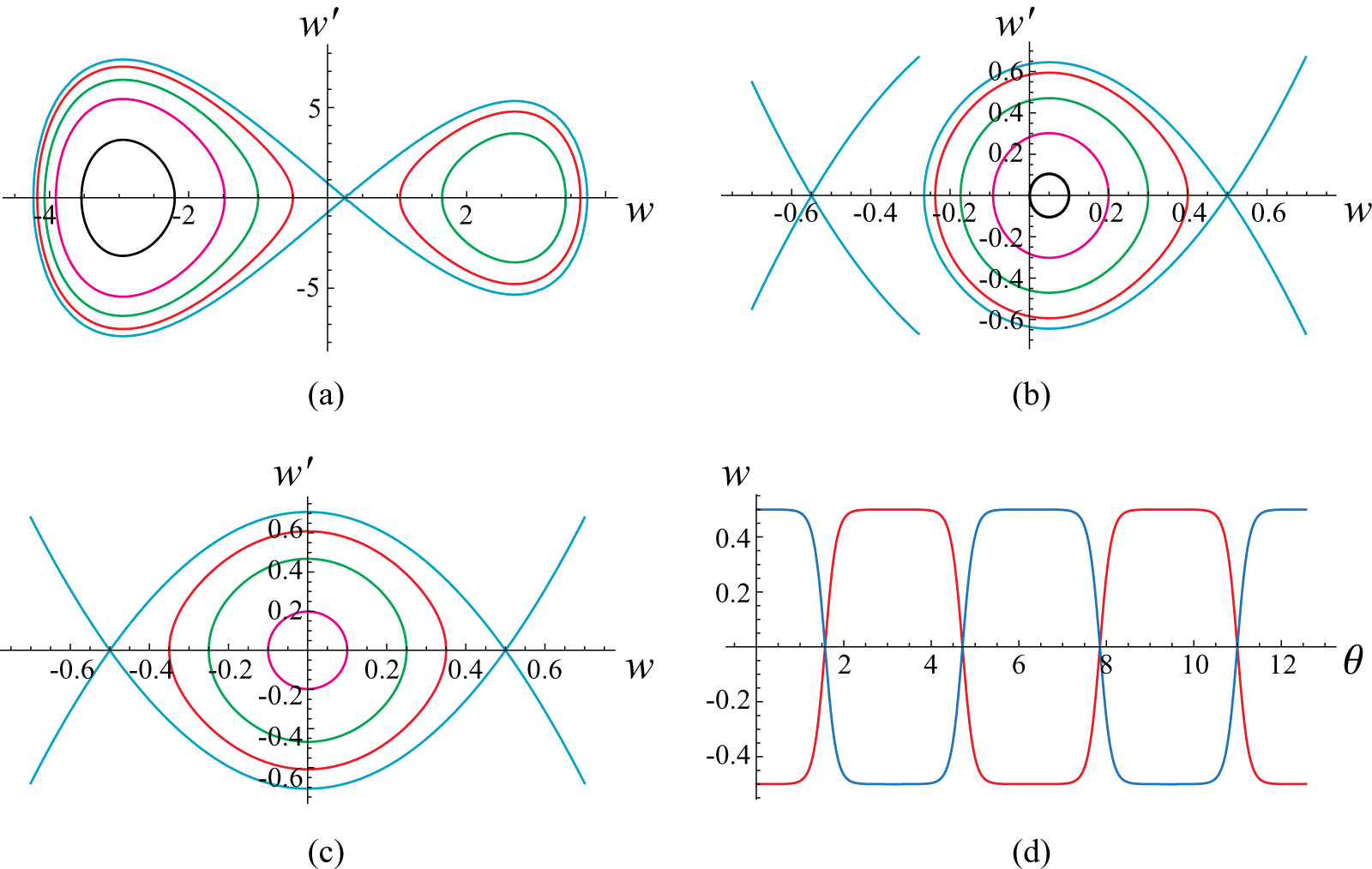


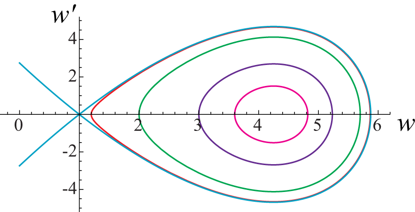


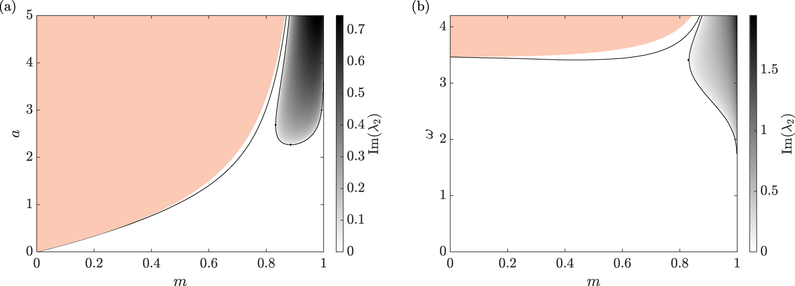


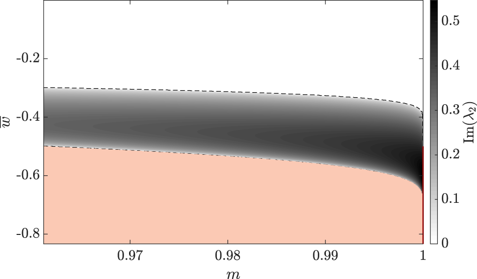


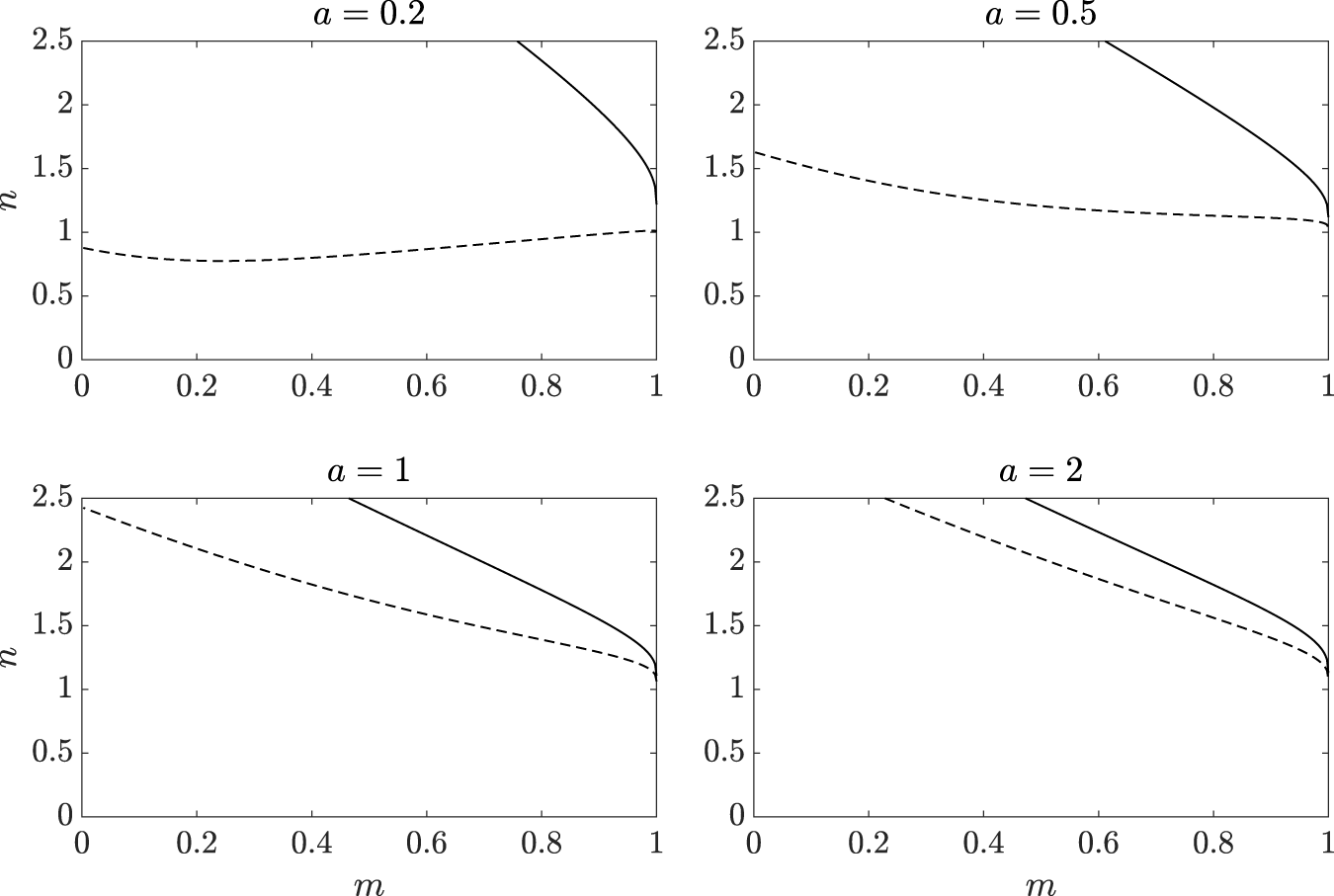


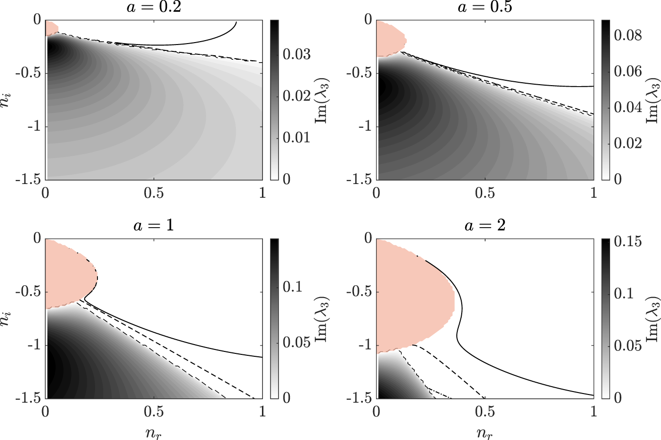


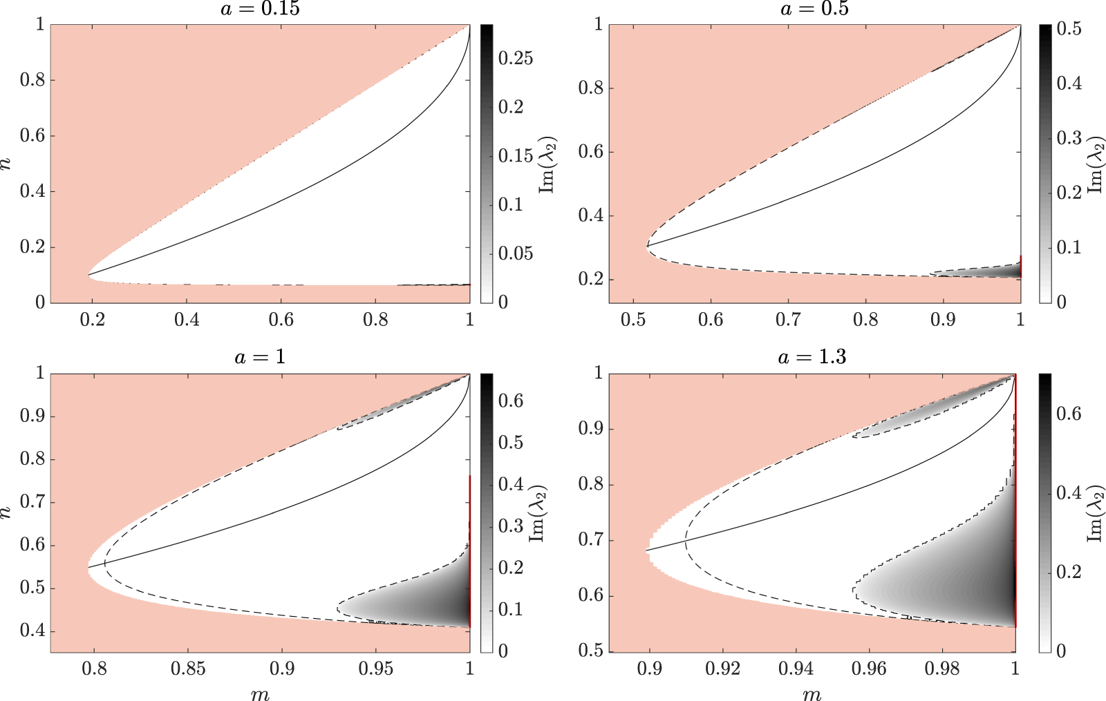


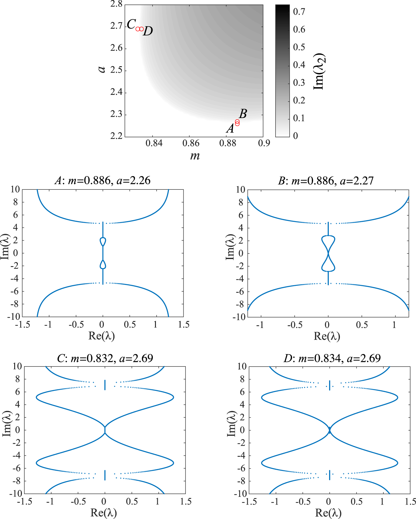


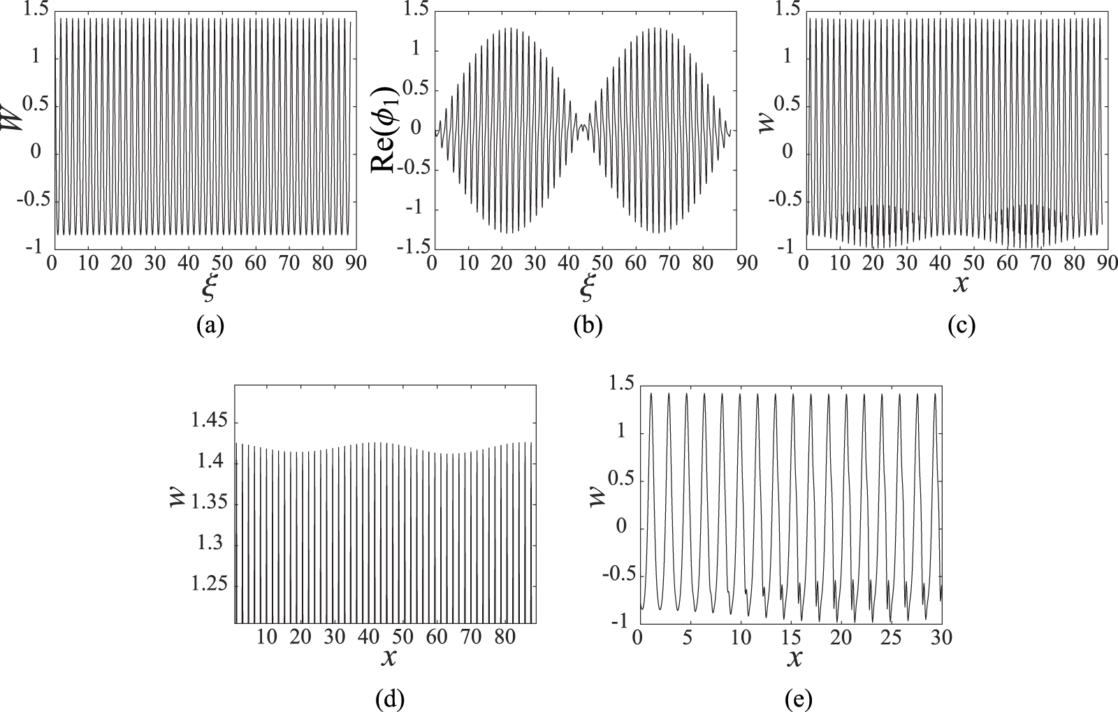


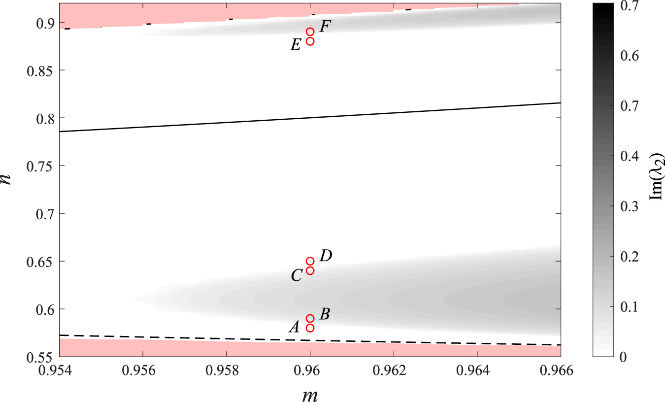


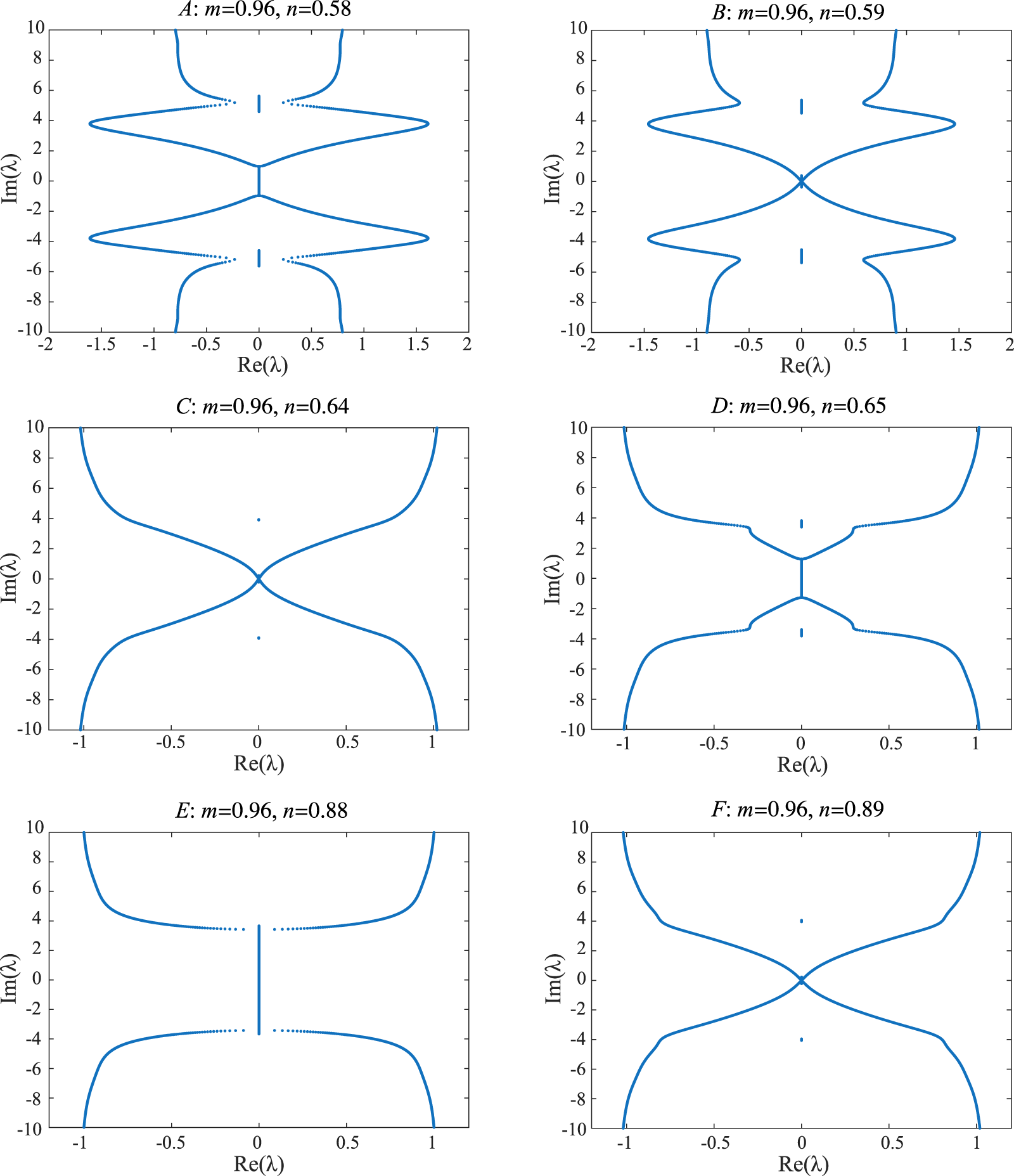


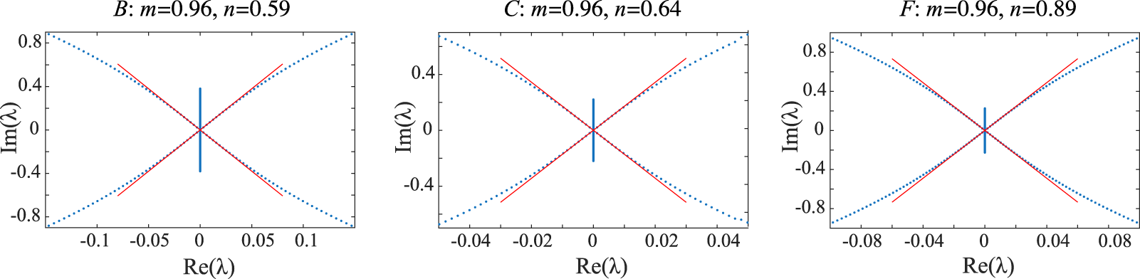


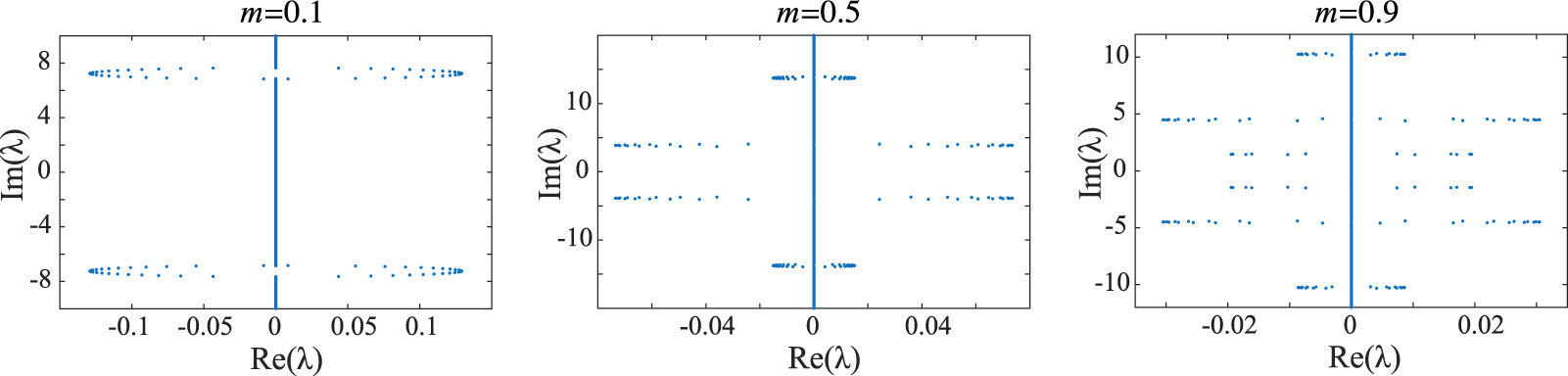


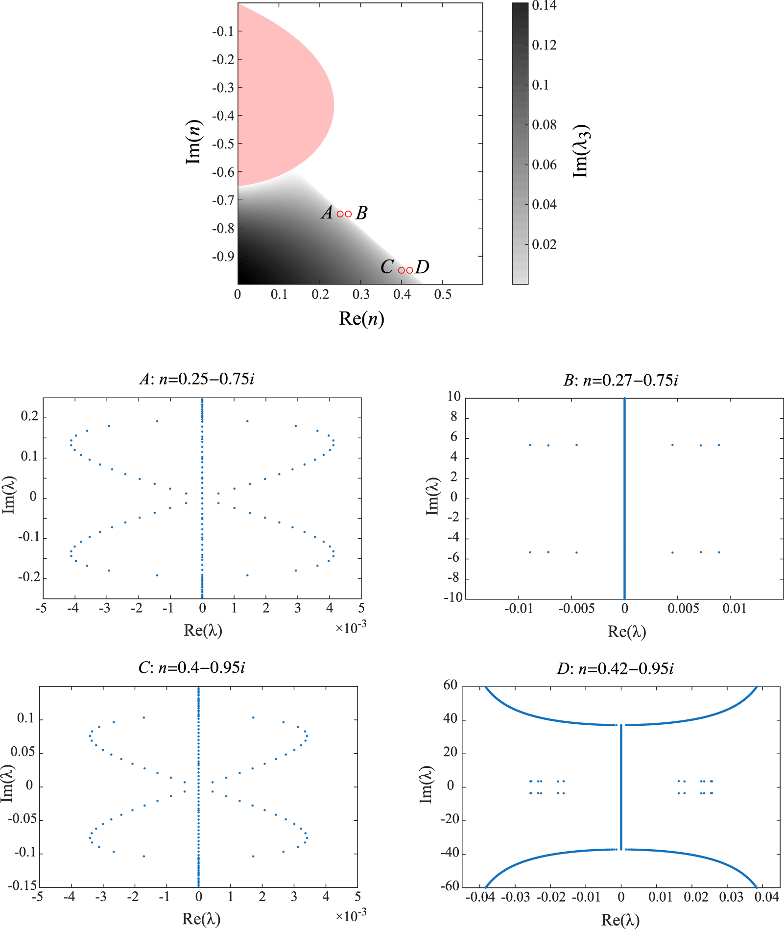


 Open access

