2.1. Spatial and temporal discretisation

The starting point is the incompressible Navier–Stokes (N–S) equations, considering a Newtonian fluid,

(2.1) \begin{gather} \dfrac {\partial u_i}{\partial x_i} = 0, \end{gather}

(2.2) \begin{gather} \dfrac {\partial u_i}{\partial t} + u_j \dfrac {\partial u_i}{\partial x_{\!j}} = -\dfrac {1}{\rho }\dfrac {\partial p}{\partial x_i} + \nu \dfrac {\partial ^2 u_i}{\partial x_{\!j} \partial x_{\!j}}, \end{gather}

where the Einstein notation is adopted. These equations are solved numerically with a highly accurate pseudo-spectral/compact finite difference code that has been used in several previous works (see Guimarães et al. Reference Harima, Fujita and Osaka2022 and references therein). The domain is a three-dimensional box, with dimensions $L_x \times L_y \times L_z$ , along streamwise, normal and spanwise directions, respectively. The number of points along each direction ( $N_x,N_y,N_z$ ) is such that grid spacings, $\Delta x = \Delta y = \Delta z$ , are uniform. The discretisation of the spatial derivatives is done using a sixth-order-compact scheme (Lele Reference Mathew and Basu1992) in the streamwise direction, $x$ , while pseudo-spectral methods are employed in the normal, $y$ -, and spanwise, $z$ -, directions, with de-aliasing done with the 2/3rd rule. The temporal advancement is performed by a third-order low storage explicit Runge–Kutta time-stepping scheme (Williamson Reference Williamson1980), combined with a fractional step method that ensures pressure–velocity coupling and incompressibility at each substep of the time-advancing scheme (Kim & Moin Reference Krogstad and Davidson1985). The outlet boundary is treated with a non-reflective outflow condition (Orlanski Reference van Reeuwijk and Holzner1976) that produces minimum distortion of the pressure field and guarantees that the coherent structures leave the computational domain without being affected. Along the normal, $y$ -, and spanwise, $z$ -, directions, periodic boundary conditions are imposed. The inflow condition is specified in the following section.

2.2. Inflow condition

The most common method to specify inflow conditions for spatially developing flows is to impose a field of random fluctuations that are divergence-free, which are then convected through the inlet plane. These disturbances, however, only mature into real, physical turbulence after travelling a considerable distance from the inlet. A better prescription of inflow turbulence would be, for example, to impose a field of random fluctuations that follow an idealised turbulence spectrum (Guimarães et al. Reference Harima, Fujita and Osaka2022) and let the frequencies contained in this noise be amplified/destroyed as the flow transitions to fully turbulent. The best alternative, however, as recognised by Moin & Mahesh (Reference Moser, Rogers and Ewing1998), is to prescribe at the inlet results from previous simulations, as realistic turbulence is found to occur at a distance significantly closer to the inlet.

Figure 1.

Energy spectrum, $E(k)$ , for each temporal homogeneous isotropic turbulence simulation: ( $\bigcirc$ ) HIT1, ( $\triangle$ ) HIT2, ( $\square$ ) HIT3,and ( $\diamondsuit$ ) HIT4. The dashed lines ( $\hbox{- - -}$ ) present the asymptotic behaviour of the spectrum in the infrared region, where $E(k)\sim k^2$ , and in the inertial range, $E(k)\sim k^{-5/3}$ . The spectra are therefore consistent with a Saffman spectrum.

The inlet condition adopted in the present work is a variation of those implemented by Tordella & Iovieno (Reference Tordella and Iovieno2011) and Cimarelli et al. (Reference Cimarelli, Cocconi, Frohnapfel and De Angelis2015) to simulate a temporal shearless mixing layer. The idea is as follows. The velocity fluctuations imposed at the inlet are extracted from a separate temporal forced homogeneous isotropic turbulence (HIT) simulation, performed on a cubic domain with triple periodic boundary conditions. This guarantees that the fluctuating velocity fields injected at the inlet are a solution of the N–S equations and follow the characteristic energy spectrum of isotropic turbulence (see figure 1). For the four temporal simulations considered (HIT1, HIT2, HIT3, HIT4), the energy spectrum has a distinct $-5/3$ slope at the inertial region, à la Kolmogorov, and the infrared region is asymptotically well described by $E(k)\sim k^2$ , consistent with a Saffman spectrum. Note that this slope is not directly prescribed, but is a consequence of the specified location of the energy peak, which itself is an input of these simulations, as detailed later this section.

The procedure to introduce the velocity fluctuations on the spatial domain can be conceptually divided into three steps.

1. (i) First, at every time step, the instantaneous $y{-}z$ velocity plane located at the middle of the temporal cube is extracted.

2. (ii) This generates inlet planes containing only the fluctuating components of the velocity field, $u^{\prime}_1$ , $u^{\prime}_2$ and $u^{\prime}_3$ . After this, a non-turbulent region with thickness $H$ is created by setting to zero the fluctuating components in the inner region of the inlet plane. As done by Cimarelli et al. (Reference Cimarelli, Cocconi, Frohnapfel and De Angelis2015), this is achieved by convolving the $u^{\prime}_1$ , $u^{\prime}_2$ and $u^{\prime}_3$ HIT planes with a hyperbolic tangent filter, see (2.3).

3. (iii) Finally, a uniform convection velocity, $U_{\infty }$ , is added and the modified HIT planes are injected at the inlet.

The concatenation of these three steps results in the following expressions to obtain the velocity components, $u_1$ , $u_2$ , $u_3$ , at $x=0$ :

(2.3) \begin{equation} \left .\begin{array}{l} u_1(x=0,y,z) = U_{\infty } + u^{\prime}_1(y,z)*\mathcal{F}(y/H) \\[0.3cm] u_2(x=0,y,z) = u^{\prime}_2(y,z)*\mathcal{F}(y/H) \\[0.3cm] u_3(x=0,y,z) = u^{\prime}_3(y,z)*\mathcal{F}(y/H) \end{array}\!\!\!\right \} \end{equation}

where

(2.4) \begin{align} \mathcal{F}(y/H)=\dfrac {1}{2}\left (1-\tanh \left [ \dfrac {1}{a} \left (1-\dfrac {2|y|}{H}\right)\right]\right) \end{align}

is the spatial filter, and $u^{\prime}_1$ , $u^{\prime}_2$ and $u_3^{\prime}$ are the velocity components extracted from the middle plane of the HIT simulation, which, by construction, correspond to the fluctuating components of the spatial simulation. We set the smoothing parameter $a=0.05$ to keep the gradient of the convolution profile sharp, while avoiding numerical noise at the inlet region (see Appendix B for a complete discussion). The parameter $H$ is the initial slot width of the non-turbulent region and is properly selected to ensure that the irrotational central region is wider than one integral length scale, eliminating correlations between the upper and lower turbulent layers.

The HIT simulations used to generate the inlet condition are carried out in a periodic cubic domain, where the governing equations are resolved with spectral accuracy in all directions. The forcing scheme, adopted from Alvelius (Reference Alvelius1999), is applied directly in the spectral space and concentrated in a range of low wavenumbers. Since, by definition, the integral scale is where most energy is contained, by controlling the spectrum peak, we have full control on the integral scale of the HIT flow. To achieve a specific Taylor-based Reynolds number, $\textit{Re}_{\lambda }$ , the magnitude of the forcing power applied, $P$ , must be conjugated with the fluid kinematic viscosity, $\nu$ , leading to

(2.5) \begin{equation} \textit{Re}_{\lambda } = \sqrt {15} \left (\dfrac {1}{3}\dfrac {L_{11} N}{C_{\varepsilon } k_{\textit{max}}\eta }\right)^{2/3} \qquad \text{and} \qquad P = \left (\frac {1}{3}\dfrac {N}{k_{\textit{max}}\eta }\right)^4 \nu ^3, \end{equation}

where $L_{11}$ is the (longitudinal) integral length scale, $N$ is the number of points of the HIT cubic grid in each direction, $C_{\varepsilon }\equiv \varepsilon L_{11}/({u^{\prime}_1}^2)^{3/2}$ is the non-dimensional energy dissipation rate and $k_{\textit{max}}\eta$ is the resolution of HIT simulation. The reader is referred to Appendix C for the complete derivation of these relations.

The significance of (2.5) lies in its ability to guide the selection of input parameters for the temporal HIT simulation, allowing precise control over the Taylor-scale Reynolds number, integral scale, and r.m.s. velocity, which would not be achievable otherwise. Moreover, this approach also allows to introduce velocity fluctuations that are temporally correlated and not ad hoc divergence-free noise.

The turbulence parameters for these temporal simulations are listed in table 1. A range of parameter magnitudes is explored, resulting in distinct turbulent energy spectra (figure 1). The four simulations were designed to have different values of r.m.s. velocity $u^{\prime}\equiv \sqrt {\overline {{u^{\prime}_1}^2}}$ , while deliberately keeping $L_{11}$ constant for simulation pairs HIT 2/HIT 3 and HIT 1/HIT 4. This set-up allows to isolate the potential concomitant effects of integral length scale and the r.m.s. velocity on TTM, as will be further discussed in § 3.

Table 1.

Parameters of the forced homogeneous isotropic turbulence (HIT) temporal simulations used to generate the inlet conditions: Taylor-scale Reynolds number ( $\textit{Re}_{\lambda }$ ); number of grid points ( $N^3$ ); r.m.s. streamwise velocity ( $u^{\prime}\equiv \sqrt {\overline {{u^{\prime}_1}^2}}$ ); enstrophy ( $\omega ^{\prime}_i \omega ^{\prime}_i$ ); forcing power input ( $P$ ); longitudinal integral scale ( $L_{11}$ ); and average resolution ( $k_{\textit{max}}\eta$ ).

At the inlet of the spatial domain, a passive scalar is injected allowing to follow non-turbulent flow. Its concentration, $\theta$ , is initialised with a top-hat profile that sets $\theta =1$ inside the non-turbulent region and $\theta =0$ in the turbulent region,

(2.6) \begin{equation} \theta (x=0,y,z) = \dfrac {1}{2}\left (1+\tanh \left [\dfrac {1}{a}\left (1-2\dfrac {|y|}{H}\right)\right]\right), \end{equation}

where $a$ acquires the same value as in (2.3). The Schmidt number is set to unity, so that the mixing scales become of the order of Kolmogorov’s length scale and thus are fully resolved.

2.3. Computational parameters of the spatial DNS

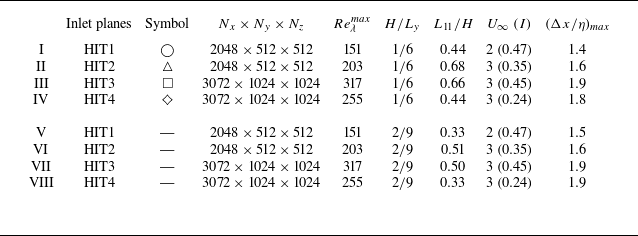
Regarding the spatial DNS, the values of physical and numerical parameters of those conducted to study turbulent/turbulent merging are summarised in table 2. For each configuration, temporal and spatial simulations are synchronised with the same (and constant) time step and the fluid properties (e.g. kinematic viscosity) are maintained from the temporal to spatial runs. These simulations can be divided in two sets (simulations I, II and III; and IV, V and VI), where only the width of the non-turbulent region, $H$ , is varied, while all other parameters are held constant. The second set of DNS (simulations IV, V and VI) is analysed only in § 3.1, for the purpose of determining the influence of the non-turbulent region width, $H$ , on the merging point location. In the remainder of this paper, only results from simulations I, II and III are presented for the sake of conciseness and to avoid duplication of similar results.

Table 2.

Physical and computational parameters of the simulations performed from left to right column-by-column: spatial simulation number; HIT simulation from which inlet planes are obtained; symbol that identifies each simulation; number of grid points of the domain along each direction $(N_x\times N_y\times N_z)$ ; Taylor-scale Reynolds number of the turbulent region at the inlet $(Re^{{max}}_{\lambda }=u^{\prime} \lambda ^{{max}}/\nu)$ ; ratio of the non-turbulent slot width to the domain size along the normal direction $(H/L_y)$ ; ratio of the integral scale of the turbulent region at the inlet to the thickness of the non-turbulent region $(L_{11}/H)$ ; convection velocity, $(U_{\infty })$ , and respective turbulence intensity, $(I=u^{\prime}/U_{\infty })$ ; and grid spacing normalised by the Kolmogorov microscale $(\Delta x/\eta)_{\textit{max}}$ , at the position where it attains its largest value.

Two examples of the resulting flowfield are depicted in figure 2, where contours of vorticity magnitude, $|\omega _i|^+=|\omega |(H/U_{\infty })$ , and passive scalar concentration, $\theta$ , sampled at the central plane, $z/H=0$ , are presented, at an illustrative instant of time. Initially, in the near-inlet region, two distinct flow regimes are clearly discernible: a central non-turbulent region, where velocity fluctuations have been removed, surrounded by turbulent inflow, extracted from HIT temporal simulations. Eventually, non-turbulent fluid is entrained into the decaying turbulent regions that grow, coalesce, merge and mix. Also, figure 2(a) evidences that the iso-vorticity structures near the inlet are stretched in the streamwise direction. This arises from the addition of a convection velocity to the HIT velocity planes that transforms the temporal correlation into a spatial one. We have verified that, in the worst case, isotropy is reattained at a distance of $1.2H$ downstream of the inlet, which corresponds to only $6\,\%$ of the domain in that direction. To avoid any ambiguities in our analysis, we always discard purposely this initial region.

Figure 2.

Two-dimensional instantaneous snapshots of (a) vorticity magnitude normalised by ( $U_{\infty }\,/\,H$ ), in $\log$ scale, and (b) passive scalar concentration, $\theta$ . Both contours are taken at the central $x{-}y$ plane ( $z=0$ ), at the same instant of time and regard simulation III. A non-turbulent region, which appears in white and black in figures (a) and (b), respectively, develops in the range of $-0.5\lt y/H\lt 0.5$ , where $\theta =1$ initially.

These snapshots (figure 2) visually suggest that ambient turbulence shreds the initially confined scalar, which is dispersed and mixed outwards. The compact scalar plume is crumbled into disjoint sheets of high values of scalar concentration, represented in dark red. Progressively, these regions of locally high concentration become less frequent and the flow evolves into a homogenised final state. Notice that, at least visually, the correlation between high-concentration regions and low-vorticity is appreciable, even for the unity Schmidt number considered, $Sc = 1$ . It is nevertheless dangerous to extend a priori this connection further and relate the geometric properties of the low-vorticity (irrotational) spots that emerge with those of scalar sheets. Enstrophy is not a passive scalar that is transported by the flow field, in the sense that its evolution reacts back on the velocity field (Sagaut & Cambon Reference Schanderl, Jenssen, Strobl and Manhart2018).

2.4. Interface detection and conditional analysis

In this work, the local analysis of TTM, conducted in § 4, relies on a correct and meaningful detection of the TNTI. The reason to reccur to conditional statistics arises from the difficulty in obtaining adequate information about the dynamics of the TNTI layer when a fixed reference frame in space and time is used (we shall refer to the latter as the ‘classical’ approach). Because the TNTI is convoluted and its position is highly intermittent, using such frame of reference to distinguish irrotational from turbulent flow turns out to be unfruitful, since a fixed frame is blind to the indentations of the irrotational boundary. Therefore, irrotational and turbulent regions will be masked and the local turbulence behaviour within the TNTI cannot be satisfactorily captured. This difficulty can be overcome by using a local, time-dependent frame of reference on top of each point of the TNTI and organising the statistics according to their local distance from the irrotational boundary (see, e.g. Bisset, Hunt & Rogers Reference Bisset, Hunt and Rogers2002).

The irrotational boundary (IB) is defined as an iso-surface of low enstrophy, whose threshold is obtained by analysing the density plot of the turbulent volume fraction of the flow (Silva et al. Reference Silva, Zecchetto and da Silva2018). Notice that, by definition, the threshold is located at the plateau of this density plot, implying that the geometry of the iso-enstrophy levels is insensitive to small variations of the threshold calculated. The points of the IB are obtained directly by interpolation of the three-dimensional enstrophy field from DNS. The local frame of reference $(x_I, y_I, z_I)$ is then constructed and aligned with the local enstrophy gradient. Accordingly, a three-dimensional normal, $y_I$ , is defined at each point of the IB (Zecchetto & da Silva Reference Zecchetto and da Silva2021), with directions $x_I$ and $z_I$ being tangent to the interface boundary, as represented in figure 3(a).

Since the three-dimensional normal is oriented towards positive enstrophy gradients, non-turbulent flow is located at $y_I\lt 0$ and rotational flow at $y_I\gt 0$ (the IB is at $y_I=0$ ). To accumulate statistics in this reference frame, the values of any field of interest are interpolated trilinearly into a grid defined along the normal and ensemble averaged according to their distance from the IB, a operation we denote as $\langle \boldsymbol{\cdot }\rangle _I$ .

Unlike most studies, we adopt the actual IB instead of the more common interface envelope, which allows the inclusion of re-entrances in the statistical sampling. Bubbles with a characteristic size smaller than $2$ grid spacings are excluded from the analysis, whether they correspond to islands of rotational flow within an irrotational region or vice versa. Depending on the Reynolds number of each case, statistics of three-dimensional fields are accumulated for a total of $80$ – $200$ time instants.

Figure 3.

(a) Illustration of the irrotational boundary (IB) and the local reference frame at an inset of a $(y,z)$ plane. (b) Domain slicing exemplified in a two-dimensional vorticity magnitude contour along the central $(x,y)$ plane. The merging region is divided into nine slices of equal thickness. These comprise regions upstream (grey gradient colour) and downstream (red gradient) of the average merging point. The colours bordering each slice will be used throughout the remainder of the paper to identify clearly each section and its respective position regarding the merging point.

Due to the decaying nature of the flow, the calculated threshold will depend on the streamwise location. To account for this, the domain is divided into nine vertical slabs of streamwise thickness $0.5H$ , covering the merging region, as depicted in figure 3(b). This analysis covers both upstream and downstream regions of the average merging location (defined later in § 3.1), and also allows to ascertain how different quantities evolve during merging. The threshold is maintained constant for each slab over different instants of time, for reasons that will become clearer in § 4, but a new threshold is calculated for each slab to accommodate the spatial evolution of the flow. In figure 4(a) and 4(b), the normalisation of the conditioned profiles by their average value at the fully turbulent region for the first slab, $\langle \boldsymbol{\cdot }\rangle ^0_T$ , clearly evidences this spatial evolution. The normal distance to the IB, $y_I$ , is normalised by the initial slot-width of the non-turbulent region, $H$ .

Figure 4.

Averaged conditional profiles of (a) enstrophy $\langle \omega _i\omega _i\rangle _I$ , (b) energy dissipation rate $\langle \varepsilon \rangle _I$ , (c) passive scalar concentration $\langle \theta \rangle _I$ and (d) local Kolmogorov length scale, $\langle \eta \rangle _I\equiv \nu ^{3/4} {\langle \varepsilon \rangle _I}^{-1/4}$ for simulation III (HIT3 inlet planes). Enstrophy and dissipation rate of kinetic energy are normalised by their value computed at the turbulent core for the first slab, $\langle \boldsymbol{\cdot }\rangle ^0_T$ , while the local Kolmogorov length scales are normalised by their value at the turbulent core for each slab, $\langle \eta \rangle _T$ . The normal distance to the IB, $y_I$ , is normalised by the initial slot width of the non-turbulent region, $H$ . The colours follow the scheme presented in figure 3.

The conditionally average enstrophy, $\langle \omega _i\omega _i\rangle _I$ , displays clearly its distinctive finite jump (Westerweel et al. Reference Westerweel, Fukushima, Pedersen and Hunt2009) and is virtually zero in the non-turbulent region. At only $y_I/H\approx 0.05$ , enstrophy has already grown to approximately its average value on the fully turbulent region. This rapid evolution occurs in just over a few Kolmogorov scales, as we will show later, and defines the TNTI.

In contrast, energy dissipation (and strain magnitude), $\langle \varepsilon \rangle _I=2\nu \langle S_{\textit{ij}} S_{\textit{ij}}\rangle _I$ , evolves much more smoothly through the IB and is non-negligible in the irrotational side (Holzner et al. Reference Holzner and Lüthi2007). The fact that irrotational flow can still dissipate turbulent kinetic energy is a manifestation of the so-called irrotational dissipation, described in great detail by da Silva & Pereira (Reference da Silva and Pereira2008). The smoothness of the strain rate can be partially interpreted by considering that $S_{\textit{ij}}S_{\textit{ij}}$ has a broader scale dependence than enstrophy, which is typically localised at the smallest scales. Notice that, in the turbulent core, strain magnitude balances enstrophy, satisfying the kinematic constraint $\langle \varepsilon \rangle _I/\nu =2\langle S_{\textit{ij}} S_{\textit{ij}}\rangle _I\approx \langle \omega _i\omega _i\rangle _I$ .

It is especially relevant to draw attention to the conditional evolution of the local Kolmogorov length scale $\langle \eta \rangle _I$ within the TNTI (see figure 4 d). The lower dissipation at the irrotational side and at the IB means that the average Kolmogorov scale in these regions is larger than at the fully turbulent core. More precisely, at the IB, $\langle \eta \rangle _I/\langle \eta \rangle _T\approx 1.7$ and, therefore, the TNTI layer is actually better resolved than the turbulent core (with the same mesh). For the simulations performed, our resolution at the interface is then $\Delta x/\eta \lesssim 1.1$ .

Over the IB, the scalar concentration, $\langle \theta \rangle _I$ , also exhibits a sharp variation, as reported in previous works (Westerweel et al. Reference Westerweel, Fukushima, Pedersen and Hunt2009). Arguably, there is a very high correlation between irrotational fluid and maximum scalar concentration. On the turbulent side, $\theta$ increases with the streamwise distance to the inlet, as a result of turbulent mixing and diffusion, while at the irrotational side, $\theta$ is practically constant and equal to one for every slab analysed. Hence, this evolution advocates for the correspondence between high concentration values and irrotational fluid, previously anticipated visually in figure 2.

These conditional profiles have been reported in many different shear flows, e.g. jets, wakes, mixing layers, boundary layers (Bisset et al. Reference Bisset, Hunt and Rogers2002; Westerweel et al. Reference Westerweel, Fukushima, Pedersen and Hunt2005; Watanabe et al. Reference Watanabe, Sakai, Nagata, Ito and Hayase2015, Reference Watanabe, da Silva and Nagata2019), and we also show here that during TTM, their qualitative overall shape is recovered.

3.1. Merging location and scalar half-width

The overall dynamics of this flow can be explained by the growth of the two initially segregated turbulent regions that entrain irrotational fluid through the TNTI, until they eventually merge. Despite this phenomenon being intermittent, in the sense that the instantaneous merging point moves back and forth, a statistical analysis shows that the distance at which they coalescence is, in essence, dependent both on the initial separation between them and the average rate at which they grow.

To detect the average merging location, the half-width of the non-turbulent region, $\delta /H$ , is calculated as a function of the streamwise coordinate, $x/H$ . Several definitions for this half-width are possible, for example, based on enstrophy (see figure 2, where the distinction between non-turbulent and turbulent regions is evident), passive scalar concentration or other less obvious quantities, each having their advantages and drawbacks.

For instance, the choice of enstrophy has the advantage of being unambiguous since, by definition, the non-turbulent region is irrotational and the turbulent has a non zero level of enstrophy, but, at the same time, has the drawback of being sensitive to the threshold value chosen, which would itself be a function of $x/H$ since the enstrophy magnitude is decaying. Notice that this threshold value is not related (directly) to the detection method of turbulent/non-turbulent interfaces. Here, we are simply concerned with computing the width of the non-turbulent region and, therefore, we consider time-averaged and not instantaneous enstrophy fields.

However, choosing the passive scalar concentration to detect the non-turbulent region is especially convenient if one considers the boundness property of the advection–diffusion equation. In this context, the choice of the scalar threshold, $\theta =0.5$ , becomes obvious. This identification is popular when scalar diffusion is small when compared with momentum diffusion or, in other words, for large Schmidt numbers. Despite the fact that this is not the case here, where $\textit{Sc}=1$ , a unity Schmidt number can prove to be well suited to trace momentum or vorticity transport. While a passive scale with $Sc\gg 1$ acts as an ideal tracer and allows to perfectly reproduce the flow kinematics, it does not capture its dynamics, which also includes diffusion effects. As will be discussed later, the proposed passive scalar threshold effectively captures the dynamics of interest (see also discussion in Appendix C). As shown in figure 4(c), the proposed passive scalar threshold of $\theta =0.5$ is actually very close to the average scalar concentration at the IB of the TNTI. Different variables, e.g. enstrophy or turbulent kinetic energy, also give similar results provided an adequate choice of their threshold value is used (see Appendix C). To exemplify the sensitivity to different scalar thresholds, an ensemble-averaged contour of scalar concentration is shown in figure 5(a), with three different iso-curves corresponding to $\theta =0.25$ , $0.5$ and $0.75$ .

Figure 5.

(a) Average scalar concentration field for simulation III. Isolines correspond to concentration levels $\theta =0.25$ , $0.5$ and $0.75$ . The inset depicts a sketch of the merging region and the streamwise evolution of the scalar half-width. (b) Normalised half-width of the non-turbulent region based on the scalar deficit, $\theta =0.5$ , for simulation VI, from table 2. Two regions are discernable: a linear one, where ${\rm d}\delta _{\theta }/{\rm d}x\approx \mathrm{const}$ , and a final one, where the half-width decays rapidly.

The scalar based half-width, $\delta _{\theta }$ , is then computed by averaging the upper and lower isocurves of scalar concentration,

(3.1) \begin{align} \frac {\delta _{\theta }}{H} (x/H) = \dfrac {1}{2}\left [y/H(\theta ^+_{0.5}) - y/H(\theta ^-_{{0.5}})\right], \end{align}

where $y/H(\theta ^+_{0.5})$ is the upper and $y/H(\theta ^-_{0.5})$ the lower $y/H$ locations where $\theta =0.5$ , for each streamwise distance $x/H$ .

By characterising the rate of entrainment into the turbulent regions, it is possible to estimate how the half-width of each turbulent layer, $\delta _T$ , evolves in space, similarly to what is often done in free shear flows. In this case, the average velocity of the turbulent stream remains constant and equal to $U_\infty$ . From mass conservation, as ilustrated in the sketch of figure 5(a), the local average entrainment velocity, $\dot {E}$ , relates to the growth of $\delta _{T}$ as

(3.2) \begin{equation} U_{\infty }(\delta _T(x+{\rm d}x) - \delta _T(x)) = \dot {E}\, {\rm d}x, \end{equation}

where $\dot {E}{\rm d}x$ denotes a mean volume flux per spanwise unit length. Rewriting (3.2) and by noting that ${\rm d}\delta _{\theta }/{\rm d}x\approx -{\rm d}\delta _{T}/{{\rm d}}x$ , the rate of entrainment can be explicitly written as

(3.3) \begin{equation} \dot {E} = -U_{\infty }\dfrac {{\rm d}\delta _{\theta }}{{\rm d}x}. \end{equation}

Now, for the purpose of this discussion, it pertinent to divide the evolution of the scalar half-width in (at least) two different regions. Figure 5(b) presents the streamwise evolution of scalar half-width, for simulation VI of table 2, and these distinct regions are suggested. Sufficiently upstream of the merging point (approximately 1.5 $H$ units of length for the case in figure 5 b), it is evident that $\delta _{\theta }/H$ varies linearly with $x/H$ , implying that ${\rm d}\delta _{\theta }/{\rm d}x\approx \mathrm{const}$ . From there until the merging point, $\delta _{\theta }/H$ approaches zero rather dramatically, with the magnitude of ${\rm d}\delta _{\theta }/{\rm d}x$ growing quickly. In the initial linear region, the simulations presented suggest that the magnitude of this slope is an increasing function of turbulence intensity. While other relationships are certainly possible, for now, we assume that a simple proportional relation holds between these quantities (which shall be promptly validated),

(3.4) \begin{align} - \dfrac {{\rm d}\delta _{\theta }}{{\rm d}x} \sim I = \dfrac {u^{\prime}}{U_{\infty }}, \end{align}

which, upon substitution of (3.3), we find

(3.5) \begin{align} \dot {E} \sim u^{\prime}, \end{align}

meaning that the (average) entrainment velocity is the same order of magnitude as the r.m.s. velocity of the turbulent layer, thus recovering the classical entrainment hypothesis (Turner Reference Turner1986; Hunt, Eames & Westerweel Reference Hussein, Capp and George2006).

It is now instructive to analyse the implications of this scaling on the merging location. Assuming that the extent of the linear region is the prevailing contribution for the merging location, or, in other words, that the rapid decay region is so fast that its contribution to the merging location can be neglected on a first approximation, (3.3) reads

(3.6) \begin{equation} \dfrac {{\rm d}\delta _{\theta }}{{\rm d}x} = - \alpha \dfrac {u^{\prime}}{U_{\infty }}, \end{equation}

where $\alpha$ is an entrainment proportionality constant, and the ratio at the right-hand side is the inlet turbulence intensity and, hence, $x\text{-independent}$ . Integrating (3.6) and dividing both sides by $H$ yields

(3.7) \begin{equation} \dfrac {\delta _{\theta }}{H} = -\alpha \dfrac {u^{\prime}}{U_{\infty }} \dfrac {x}{H} + C_0, \end{equation}

where $C_0 \equiv 1/2$ is the initial half-width non-dimensionalised by $H$ . The merging point location, $x_{\textit{merg}}$ , is estimated by equating $\delta _{\theta }$ to zero in (3.7),

(3.8) \begin{equation} x_{\textit{merg}} \sim U_{\infty } H/u^{\prime}, \end{equation}

where $\alpha$ was considered constant and, by hypothesis, independent of the initial turbulence parameters. Hence, globally and on average, large-scales govern entrainment. Specifically, the turbulence intensity dictates the ratio between entrainment and average convection velocities (and therefore sets the slope of the linear region ${\rm d}\delta _{\theta }/{\rm d}x$ ). Indeed, from (3.8), the merging locations collapse when the streamwise coordinate $x$ is appropriately rescaled (see table 3),

(3.9) \begin{equation} x \to \dfrac {x}{H} \dfrac {u^{\prime}}{U_{\infty }} \equiv x^+. \end{equation}

Interestingly, and despite the fact that integral length scales have a clear influence on the intermittent penetration across the two layers in the case of turbulent mixing layers (Veeravalli & Warhaft Reference Veeravalli and Warhaft1989; Tordella & Iovieno Reference Tordella and Iovieno2006), this does not translate into an evident influence on the global entrainment rate (or, by extension, on the merging point location), at least for the range considered in this work, as presented in table 3.

Table 3.

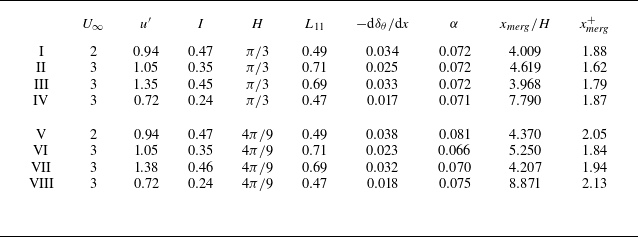
Location of the merging point, ( $x_{\textit{merg}}/H$ ) and its rescaled value ( $x_{\textit{merg}}^+$ ), for simulations in table 2. The columns present the convection velocity $(U_{\infty })$ ; r.m.s. streamwise velocity at the inlet $(u^{\prime})$ ; turbulence intensity of the inflow $(I)$ ; initial slot width of the non-turbulent flow normalised by the domain size in the normal direction $(H)$ ; longitudinal integral scale calculated near the inlet $(L_{11})$ ; the average slope of scalar half-width in the linear region ( $-{\rm d}\delta _{\theta }/{{\rm d}}x$ ); and the entrainment proportionality constant $(\alpha)$ , as defined in (3.6).

The combined influence of turbulence intensity and integral scale can be quantified by considering that a generic situation, where the entrainment rate (as measured by ${\rm d}\delta _{\theta }/{\rm d}x$ in the linear region) is a function $F()$ of these two separate variables, can be condensed into a single variable that encompasses both contributions (Kankanwadi & Buxton Reference Kim and Moin2020). Under such assumption, it follows that

(3.10) \begin{align} \dfrac {{\rm d}\delta _{\theta }}{{\rm d}x} = F\left (\dfrac {u^{\prime}}{U_{\infty }},\dfrac {L_{11}}{H} \right)\!, \quad \text{simplifies to} \; \dfrac {{\rm d}\delta _{\theta }}{{\rm d}x} = F\left ( \left (\dfrac {u^{\prime}}{U_{\infty }}\right)^{\! m} \left (\dfrac {L_{11}}{H}\right)^{\! n} \right)\!. \end{align}

Equation (3.10) can be rewritten conveniently as

(3.11) \begin{equation} \frac {{\rm d}\delta _\theta }{{\rm d}x} = A \left (\dfrac {u^{\prime}}{U_{\infty }}\right)^{\! m} \left (\dfrac {L_{11}}{H}\right)^{\! n} \!, \end{equation}

where $A$ , $m$ and $n$ are fitting parameters. (We neglect a possible summation prefactor, i.e. we consider the lower bound of ${\rm d}\delta _\theta /{\rm d}x$ to be zero.) By taking the $\log$ on both sides, one finds

(3.12) \begin{align} \underbrace { \log ({\rm d}\delta _\theta /{{\rm d}x}) - \log (A) - m\log (u^{\prime}/U_{\infty }) - n\log (L_{11}/H)}_{Q} = 0, \end{align}

which is an adequate form to calculate the values of $A$ , $m$ and $n$ that minimise the accumulated residual ( $Q^2$ ). For the data in table 3, we find

(3.13) \begin{align} \log (A)=-2.35, \quad m = 1.08 \quad \text{and} \quad n=-0.13, \end{align}

with the accumulated residual $\sum _{1}^{8}Q^2\sim 10^{-5}$ and a coefficient of determination $R^2=0.97$ for the total eight DNS carried out.

Hence, the inflow turbulence intensity is the key quantity (around eight times more predominant than the integral scale) to characterise the entrainment rate in this flow. Moreover, the value of $m$ close to unity supports the reasonability of the linear approximation (3.6) to scale the merging point, as also evidenced by the approximate constancy of $\alpha$ for the different simulations (see table 3). In fact, fixing the fitting exponents to $m=1$ and $n=0$ only reduces the coefficient of determination to $R^2=0.95$ . This diminished role of the integral length scale on the mean mass flux is consistent with previous findings for turbulent entrainment into a cylinder wake (Kankanwadi & Buxton Reference Kim and Moin2020).

The form of (3.9) and, in general, the scaling here presented for the merging point is reminiscent of the dilution length defined by Villermaux & Rehab (Reference Villermaux and Rehab2000) for mixing in coaxial jets. In a similar fashion, this length is also found to be proportional to the initial slot width (here denoted by $H$ ) and a velocity ratio that describes the entrainment rate (in this case, $u^{\prime}/U_{\infty }$ ). When mean shear is present, e.g. mixing layers, entrainment is satisfactorily characterised by a different ratio involving the mean velocities of the two streams (Brown & Roshko Reference Brown and Roshko1974). Therefore, extensions of this scaling to account for the influence of mean shear on the average merging point can easily be performed.

3.2. Turbulent kinetic energy

As the two turbulent layers grow and approach each other, velocity fluctuations are induced in the central (and initially irrotational) region. This is well represented in figure 6, where the spatial evolution of turbulent kinetic energy, $\mathcal{K}=\overline {u^{\prime}_iu^{\prime}_i}/2$ , is displayed over the centreline, $y/H=0$ , as the flow transitions from non-turbulent to turbulent, for three of the spatial simulations considered (I, II and III of table 2).

In general, the intensity of these velocity fluctuations grows sharply upstream of the merging point and decays downstream. Figure 6 also allows for a physical interpretation of the average merging location: it is a maximum of turbulent kinetic energy. As will be discussed later, this is a manifestation of the mechanisms of energy transfer between rotational and irrotational fluid. We highlight that using this maximum to define the merging point is consistent with previous observations for merging twin free jets, namely hot wire data from Harima et al. (Reference Holzner, Liberzon, Nikitin, Kinzelbach and Tsinober2005) and numerical simulations by Taddesse & Mathew (Reference Taddesse and Mathew2022), which report a maximum of turbulence intensity at the merging point of the two jets, defined by the intersection of their outer shear layers. Therefore, the scaling here presented is also expected to be successful for describing merging in free-shear flows.

At the same time, this evidences the very close relation between the passive scalar evolution, from which the merging point is detected ( $\delta _{\theta }=0$ ), and the turbulence parameters of the flowfield. The dispersion of the concentration field of passive scalar in turbulent flows is known to be closely related to the large scales of the turbulent inflow (Villermaux & Innocenti Reference Villermaux and Innocenti1999), as the scaling of the merging point evidences in this case (see (3.9)). Therefore, it is not surprising that large-scale quantities, such as turbulent kinetic energy, are well described when rescaled in relation to the merging point. The importance of the merging location in the overall dynamics of this flow is further confirmed by the fact that the evolution of $\mathcal{K}$ collapses satisfactorily when scaled with its value at merging and plotted against $x^+$ , where the merging location is universal.

Figure 6.

Streamwise evolution along the centreline of turbulent kinetic energy, $\mathcal{K}$ , normalised by the kinetic energy at the merging point, $\mathcal{K}_{\textit{merg}}$ . Simulations ( $\bigcirc$ ) I (HIT 1 inlet planes), ( $\triangle$ ) II (HIT 2 inlet planes), ( $\square$ ) III (HIT 3 inlet planes), and ( $\diamondsuit$ ) IV (HIT 4 inlet planes). The ensemble averaged normalised location of the merging point, $x^+_{\textit{merg}}$ , is marked with a dashed vertical line and the very-near-inlet region is not represented. The inset displays the evolution on a logarithmic scale in both axes ( $\log$ – $\log$ scale).

Let us now consider the evolution of $\mathcal{K}$ sufficiently downstream, i.e. $x^+\approx 4$ . In this region, homogeneity is reattained and a free decay evolution is recovered,

(3.14) \begin{equation} \dfrac {\mathcal{K}}{\mathcal{K}_{\textit{merg}}} \sim (x^{+})^{-n}. \end{equation}

This is evidenced by the $\log$ – $\log$ inset of figure 6, where $\mathcal{K}$ evolution closely follows a Saffman decay, with exponent $n=6/5$ . This result is in perfect agreement with numerical and experimental reports of energy decay in grid turbulence (e.g. Krogstad & Davidson (Reference Laban, Aleyasin, Tachie and Koupriyanov2011)), provided that the infrared region of the energy spectrum is well approximated by a Saffman spectrum, as illustrated in figure 1.

Hence, along the centreline, TTM is characterised by three distinct regions: (i) build-up of kinetic energy until the merging point; (ii) mixing/merging buffer region; and (iii) a free-decay regime, where turbulence behaves similarly to grid turbulence.

Figure 7.

Streamwise evolution along the centreline of turbulent kinetic energy associated with each component, $\overline {u^{\prime}_1u^{\prime}_1}$ in red, $\overline {u^{\prime}_2u^{\prime}_2}$ in green and $\overline {u^{\prime}_3u^{\prime}_3}$ in blue, normalised by their value at the merging point. Simulations ( $\bigcirc$ ) I (HIT 1 inlet planes), ( $\triangle$ ) II (HIT 2 inlet planes), ( $\square$ ) III (HIT 3 inlet planes) and ( $\diamondsuit$ ) IV (HIT 4 inlet planes). The ensemble averaged normalised location of the merging point, $x^+_{\textit{merg}}$ , is marked with a dashed vertical line. The top-left inset details the evolution of each component in the region upstream of the average merging point, while at the top-right, the downstream region is depicted. Both insets have a logarithmic scale in both axes ( $\log$ – $\log$ scale).

In the first region, one notable consequence of the turbulent streams approaching each other is the induction of anisotropic velocity fluctuations in the inner irrotational region (see details in figure 7). All three diagonal components of the Reynolds stresses ( $\overline {u^{\prime}_1u^{\prime}_1}$ , $\overline {u^{\prime}_2u^{\prime}_2}$ and $\overline {u^{\prime}_3u^{\prime}_3}$ ) increase up to the merging location $x^+_{\textit{merg}}$ . Among them, $\overline {u^{\prime}_1u^{\prime}_1}$ and $\overline {u^{\prime}_2u^{\prime}_2}$ peak closer to the merging point, while interestingly, $\overline {u^{\prime}_3u^{\prime}_3}$ reaches its maximum farther downstream.

Within this region, the dominant component is $\overline {u^{\prime}_2u^{\prime}_2}$ . This behaviour can be understood by considering the evolution of energy across a ‘classical’ TNTI, assuming the turbulent streams are still sufficiently separated such that their mutual interaction is negligible. Under such assumption, the streamwise component $\overline {u^{\prime}_1u^{\prime}_1}$ decays much faster than the cross-stream component $\overline {u^{\prime}_2u^{\prime}_2}$ across the TNTI, leading to the dominance of the latter in the irrotational region (Xavier et al. Reference Xavier, Teixeira and da Silva2021).

In turn, if the focus is placed on the growth rather than the absolute magnitude, figure 7 shows that the streamwise component exhibits the most significant increase from the inlet to the merging point. These dissimilarities between the energy present in each velocity component can be analysed by examining their respective turbulent kinetic energy budgets. Assuming $\partial /\partial y \gg \partial /\partial x$ , the equations simplify as follows (a full evaluation of each term will follow later, see (3.16)):

(3.15) \begin{equation} \left .\begin{array}{ll} x:& \qquad U_{\infty } \dfrac {\partial }{\partial x} \left (\dfrac {1}{2} \overline {u^{\prime}_1u^{\prime}_1} \right) \approx \dfrac {\partial }{\partial y} \left (-\dfrac {1}{\rho } \overline {p^{\prime}u^{\prime}_2} -\dfrac {1}{2} \overline {u^{\prime}_1u^{\prime}_1u^{\prime}_2}\right) - \varepsilon _x, \\[0.3cm] y:& \qquad U_{\infty } \dfrac {\partial }{\partial x} \left (\dfrac {1}{2} \overline {u^{\prime}_2u^{\prime}_2} \right) \approx \dfrac {\partial }{\partial y} \left (-\dfrac {1}{\rho } \overline {p^{\prime}u^{\prime}_2} -\dfrac {1}{2} \overline {u^{\prime}_2u^{\prime}_2u^{\prime}_2}\right) - \varepsilon _y, \\[0.3cm] z:& \qquad U_{\infty } \dfrac {\partial }{\partial x} \left (\dfrac {1}{2} \overline {u^{\prime}_3u^{\prime}_3} \right) \approx \dfrac {\partial }{\partial y} \left (-\dfrac {1}{\rho } \overline {p^{\prime}u^{\prime}_2} -\dfrac {1}{2} \overline {u^{\prime}_3u^{\prime}_3u^{\prime}_2}\right) - \varepsilon _z,\\ \end{array}\!\!\!\right \} \end{equation}

where $(\boldsymbol{\cdot })^{\prime}$ denotes the fluctuating component of each variable, after the Reynolds decomposition, and $(\varepsilon _x,\varepsilon _y,\varepsilon _z)$ are the contributions of turbulent kinetic energy dissipation associated with each velocity component (e.g. $\varepsilon _x=2\nu \overline {s^{\prime}_{1j}s^{\prime}_{1j}}$ ). Averages are taken along the homogeneous spanwise direction $z$ and time; hence, $\partial \overline {(\boldsymbol{\cdot })}/\partial z=0$ and $\partial \overline {(\boldsymbol{\cdot })}/\partial t = 0$ . Note also that in (3.15), the viscous diffusion and turbulent kinetic energy production by mean shear have been neglected, anticipating the results from the full analysis.

The first term on the right-hand side of (3.15) (pressure–velocity redistribution) is common to all three components and therefore contributes equally to both streamwise and cross-stream fluctuations. The dissipation terms are associated with the (more isotropic) small-scale motions, thus are assumed to be of similar magnitude. The turbulent transport terms that remain are notably different. Consistent with the observation that $\overline {u^{\prime}_1u^{\prime}_1}$ decreases more rapidly than the cross-stream components away from the TNTI, the turbulent transport associated with streamwise fluctuations is expected to be more intense. From (3.15), the streamwise variation of $\overline {u^{\prime}_1u^{\prime}_1}$ is therefore more pronounced in the early region.

The stages of merging become more evident once each of the turbulent kinetic energy transfer mechanisms are analysed. The full evolution equation for turbulent kinetic energy, $\mathcal{K}=\overline {u^{\prime}_iu^{\prime}_i}/2$ , allows to detail the role of each term for the generation of turbulence in the core region and reads (without any simplifications for this flow configuration)

(3.16) \begin{align} U_{\infty } \dfrac {\partial }{\partial x} \left (\dfrac {1}{2}\overline {u^{\prime}_iu^{\prime}_i}\right) = &\dfrac {\partial }{\partial x_{\!j}} \bigg (\underbrace {-\dfrac {1}{\rho } \overline {p^{\prime}u^{\prime}_{\!j}}}_{\text{Pressure-velocity}} \underbrace {+2\vphantom {\dfrac {1}{\rho }}\nu \overline {u^{\prime}_i s^{\prime}_{\textit{ij}}}}_{\text{Diffusion}}\underbrace {-\vphantom {\dfrac {1}{\rho }}\dfrac {1}{2}\overline {u^{\prime}_iu^{\prime}_iu^{\prime}_{\!j}}}_{\text{Turbulent transport}}\bigg) \\ \nonumber & \underbrace {-\overline {u^{\prime}_iu^{\prime}_j}\dfrac {\partial \overline {u_i}}{\partial x_{\!j}}}_{\text{Production}}\hspace {0.2cm} - \underbrace {2\nu \vphantom {\dfrac {\partial \overline {u_i}}{\partial x_{\!j}}}\overline {s^{\prime}_{\textit{ij}} s^{\prime}_{\textit{ij}}}}_{\text{Dissipation},\,\varepsilon }, \end{align}

where $s^{\prime}_{\textit{ij}}= ({1}/{2}) (\partial u^{\prime}_i/\partial x_{\!j} + \partial u^{\prime}_j/\partial x_i)$ is the fluctuating rate of strain. The left-hand side is the total variation of $\mathcal{K}$ (by advection) and all budgets that represent local sources or sinks of kinetic energy are placed at the right-hand side. Due to the spatial dimension of the simulations, the index $j$ covers the streamwise direction $x$ and the inhomogeneous direction $y$ . Average spanwise $z$ and time derivatives are null for the same reason as in (3.15).

Figure 8.

Turbulent kinetic energy budgets evaluated at consecutive downstream $x^+$ stations: (a) $x^+=1.5$ ; (b) $x^+=2.0$ ; (c) $x^+=3.0$ and (d) $x^+=4.5$ . The results correspond to the spatial simulation II. From left to right, column-by-column, the legend refers to: turbulent kinetic energy dissipation rate, production, viscous diffusion, advection (which is the sum of all remaining terms), turbulent transport and pressure–velocity correlation. All terms are normalised by the average energy dissipation at the merging point. The scale is maintained for all $x^+$ stations.

The contribution of each term along profiles in the normal direction, $y$ , is depicted in figure 8. The budgets are sampled at various $x^+$ sections and regard simulation II (HIT2 inlet planes). Very similar results were obtained for the other spatial simulations, but are omitted for the sake of brevity. After the value of each term is normalised by the magnitude of dissipation at the merging point, these curves also collapse at equal $x^+$ locations. The level of convergence of the terms in (3.16) is not perfect, but it is adequate to draw conclusions about energy transfer mechanisms. Specifically, larger-scale budgets, such as pressure–velocity redistribution and turbulent transport exhibit less smooth profiles than dissipation rate, which is dominated by small-scale dynamics.

Recall that, by construction, turbulent and non-turbulent flow are convected with equal velocity $U_{\infty }$ ; hence, (3.16) can be further simplified. It is straightforward to realise that the production term must be zero at every $x^+$ station, since there is no mean shear, i.e. $\partial \overline {u_i}/\partial x_{\!j} = 0$ . This absence of turbulent kinetic energy production is indeed confirmed by the results obtained, see figure 8, where for all stations, production is virtually zero. Over the normal direction, viscous diffusion of energy is also negligible at all locations.

At the turbulent regions, $|y|/H\gtrsim 0.5$ , the contribution of turbulent transport and pressure–velocity correlation is negligible on average, which is characteristic of HIT, being a direct consequence of mass conservation and isotropy. The dissipation rate of turbulent kinetic energy, $\varepsilon$ , along this region decreases for progressively downstream locations, evidencing the spatial turbulence decay. In the inner region, where the flow is initially non-turbulent, turbulence is induced by the turbulent transport term, whose contribution surpasses the losses caused by a depleted dissipation rate (with respect to the turbulent region) and pressure–velocity redistribution, which are both negative in this region. The prevailing contribution for turbulent transport comes from the derivatives along the normal direction, in which the flow is highly inhomogeneous. Consequently, the transport of turbulence by turbulence itself is responsible for a streamwise increase of kinetic energy, which is notorious in the first station analysed, $x^+=1.5$ , which is located upstream of the merging point. Sufficiently downstream of merging (see budgets regarding section $x^+=4.5$ in figure 8), turbulence spreads and the flow is homogenised. The spatial variation of kinetic energy becomes exclusively dictated by the dissipation rate and all the other contributions are negligible, leading to the free decay reported previously,

(3.17) \begin{equation} \dfrac {D\mathcal{K}}{Dt} = U_{\infty } \dfrac {\partial }{\partial x} \left (\dfrac {1}{2} \overline {u^{\prime}_i u^{\prime}_i}\right) \approx - \varepsilon . \end{equation}

Furthermore, because kinetic energy has a maximum at $x^+_{\textit{merg}}$ , one has that $D\mathcal{K}/Dt$ must be zero at merging. Since production and viscous diffusion are negligible throughout the merging event, (3.16) evidences that, to be a maximum, an equilibrium among turbulent transport, pressure–velocity and dissipation rate terms must suffice at the merging point,

(3.18) \begin{equation} \dfrac {\partial }{\partial x_{\!j}} \left (\dfrac {1}{2}\overline {u^{\prime}_iu^{\prime}_iu^{\prime}_j}\right) = - \dfrac {\partial }{\partial x_{\!j}}\left (\dfrac {1}{\rho }\overline {p^{\prime}u^{\prime}_j}\right) - \varepsilon . \end{equation}

In other words, at this point, the r.m.s. velocities in the inner region have grown enough so that the dissipation rate has increased (in absolute value) and turbulent transport has decreased just in the right amount for the aforementioned balance to hold.

The trajectory along the phase of turbulent transport and pressure–velocity contributions is depicted in figure 9, at the four $x^+$ stations considered. The arrow points in the direction of increasing $x^+$ , or for a given streamwise location, indicates increasing $|y|/H$ . Therefore, in any case, the arrow is indicative of increasing turbulence intensity, either by travelling along the normal direction, at a constant $x^+$ , from the non-turbulent core to the surrounding turbulent region, or by travelling along the centreline from the initial non-turbulent flow towards the merging region.

Figure 9.

Trajectories of pressure–velocity and turbulent transport of turbulent kinetic energy, at different $x^+$ stations, for simulation II. The dashed line indicates the preferred direction along which points lie, $\text{(turbulent transport)}=-3\,\text{(pressure}{-}\text{velocity)}$ .

There is an evident anti-correlation between these two terms, across all $x^+$ stations both in the inner (initially non-turbulent) and outer (turbulent) regions. The most extreme events, appearing as maxima (minima) of turbulent transport (pressure–velocity) terms occur at the most upstream sections of the inner region, where the contribution of turbulent transport to increase energy is approximately three times greater in magnitude than the loss provoked by pressure–velocity diffusion. Therefore, the trajectory to merging corresponds to a linear descent (along the direction of the arrow in figure 9) in the phase space, which follows approximately $(\text{pressure}{-}\text{velocity})\approx -1/3 (\text{turbulent transport})$ . From (3.18), it is straightforward to estimate that energy dissipation should account for the remaining $2/3$ of turbulent transport at the merging point. The anti-correlation of turbulent–turbulent interactions and pressure–velocity redistribution is transversal to different sorts of turbulent flows: mixing layers (Veeravalli & Warhaft Reference Veeravalli and Warhaft1989), jets (Hussein, Capp & George Reference Kankanwadi and Buxton1994) and bluff-body wakes (Schanderl et al. Reference da, Carlos, Hunt, Eames and Westerweel2017).

4.1. Conditional enstrophy, enstrophy budgets and entrainment velocity

The conditional enstrophy evolution has been presented in figure 4, but once these profiles are normalised by the average local Kolmogorov scales ( $\eta _I$ and $u_{\eta _I}$ ), as proposed by Zecchetto & da Silva (Reference Zecchetto and da Silva2021), the TNTI becomes much clearer. To compute the thickness of the vorticity jump, we define a limit value for the derivative ${\rm d}(\omega _i\omega _i)/{\rm d}y_I$ of 25 % of its maximum, following Watanabe et al. (Reference Watanabe, Riley and Nagata2017, Reference Watanabe, da Silva and Nagata2019). This thickness, which delimits the TNTI, has an average value across the nine slabs analysed of $\langle \delta _I \rangle =13\eta _T=10\eta _I$ (note the difference between turbulent and local Kolmogorov micro-scales), which is in good agreement with previous works (Taveira & da Silva Reference Taveira and da Silva2014; Silva et al. Reference Silva, Zecchetto and da Silva2018). Figure 10 confirms that $\langle \delta _I \rangle$ coincides with the peak of normalised enstrophy.

Furthermore, these non-dimensional conditional profiles collapse for $y_I/\eta _I\gtrsim 35$ . At large distances from the IB, kinematic constraints enforce

(4.1) \begin{equation} \left \langle \dfrac {\omega _i\omega _i}{(u_{\eta }/\eta)^2}\right \rangle _I \to 1. \end{equation}

We recall that this is exactly the same constraint obeyed by strain magnitude and enstrophy, highlighted in § 2.4, that is imposed by homogeneity considerations.

Figure 10.

Averaged conditional profiles of enstrophy magnitude normalised by local Kolmogorov scales, $\langle \eta \rangle _I$ and $\langle u_{\eta } \rangle _I$ . The two vertical lines delimit the average width of the TNTI, $\langle \delta _I \rangle$ . The curves correspond to simulation III and follow the colour scheme presented in § 2.4.

The most interesting phenomenon is concentrated at the region immediately adjacent to the IB (i.e. $0\lt y_I/\eta _I\lesssim 35$ ), where the normalised enstrophy profiles do not collapse. As the two turbulent layers merge, the peak of $\langle \omega _i\omega _i/(u_{\eta }/\eta)^2\rangle _I\approx 1.25$ initially located at $y_I/\eta _I\approx 10$ decreases and is displaced closer to the IB, as evidenced in the inset of figure 10. For instance, the last slab analysed exhibits its peak at $y_I/\eta _I\approx 8$ , where $\langle \omega _i\omega _i/(u_{\eta }/\eta)^2\rangle _I\approx 1.18$ . This can be better understood based on the following analytical argument. Consider the normalisation of enstrophy by the local Kolmogorov scales,

(4.2) \begin{equation} \bigg \langle \dfrac {\omega _i\omega _i}{(u_{\eta }/\eta)^2}\bigg \rangle _I = \dfrac {\langle (\partial u_i/\partial x_{\!j})^2\rangle _I - \langle (\partial u_i/\partial x_{\!j})(\partial u_j/\partial x_i) \rangle _I}{\langle (\partial u_i/\partial x_{\!j})^2\rangle _I + \langle (\partial u_i/\partial x_{\!j})(\partial u_j/\partial x_i)\rangle _I}. \end{equation}

Clearly, values of normalised enstrophy larger than one (as occurs in the peak) are a consequence of $\langle (\partial u_i/\partial x_{\!j})(\partial u_j/\partial x_i) \rangle \lt 0$ , which is only possible if the flow is not homogeneous (Taylor Reference Taylor1938).

Figure 11.

Probability density function (p.d.f.) of the alignment between the interface normal, $y_I$ , and the fixed reference frame versors (a) $\boldsymbol{e_x}$ , (b) $\boldsymbol{e_y}$ and (c) $\boldsymbol{e_z}$ . The curves correspond to simulation III and follow the colour scheme presented in § 2.4.

Based on this, as merging occurs, its effect is to homogenise the flow in the immediate proximity of the irrotational boundary, $y_I/\eta _I\approx 10$ , where the flow is inherently inhomogeneous. Therefore, during merging, we depart from the typical TNTI and non-turbulent fluid becomes organised in bubbles that are surrounded by homogeneous turbulence. This effect is evident by the loss of preferential orientation of the interface, as presented in figure 11, where the probability density function (p.d.f.) of the alignment between $y_I$ and each base direction $(x,y,z)$ is presented. While for the most upstream sections it is highly probable that the interface normal $y_I$ is aligned with the domain normal direction, $y$ , i.e. it is more likely that $|\cos (y_I\boldsymbol{\cdot }\boldsymbol{e_y})|\gt 0.5$ than its opposite, for sections downstream, this behaviour is greatly reduced, suggesting the appearance of pockets of irrotational fluid without a preferential alignment. In fact, after merging, the probability of the interface normal being perfectly aligned with the $y$ direction is lower than that with the other two directions.

To complement the analysis of enstrophy, we now consider the evolution of its budgets. Applying a conditional average to the enstrophy transport equation yields

(4.3) \begin{equation} \left \langle \dfrac {\rm D}{{\rm D}t} \left (\dfrac {\omega _i\omega _i}{2}\right) \right \rangle _I = \underbrace {\vphantom {\dfrac {\partial \omega _i}{\partial x_{\!j}}}\langle \omega _i\omega _jS_{\textit{ij}}\rangle _I}_{\text{Production}} + \underbrace {\left \langle \nu \dfrac {\partial ^2}{\partial x_{\!j}\partial x_{\!j}}\left (\dfrac {\omega _i\omega _i}{2}\right)\right \rangle _I}_{\text{Diffusion}} - \underbrace {\left \langle \nu \left (\dfrac {\partial \omega _i}{\partial x_{\!j}} \dfrac {\partial \omega _i}{\partial x_{\!j}}\right)\right \rangle _I}_{\text{Dissipation}} \end{equation}

(which is only near-exact, since it considers that the interface moves at a constant speed (Westerweel et al. Reference Westerweel, Fukushima, Pedersen and Hunt2009)). The evolution of the right-hand side terms of (4.3) is depicted in figure 12, after normalisation with local Kolmogorov scales.

Figure 12.

Averaged conditional profiles of enstrophy budgets normalised by local Kolmogorov scales, $\langle \eta \rangle _I$ and $\langle u_{\eta } \rangle _I$ . ( $\hbox{- - -}$ ) enstrophy production, $\langle \omega _i \omega _j S_{\textit{ij}} \rangle _I$ ; ( $\hbox{$\cdots\cdots$}$ ) enstrophy diffusion; and ( $\hbox{- $\cdot$ - $\cdot$}$ ) enstrophy dissipation, as defined in (4.3). VSL stands for viscous superlayer and TSL for turbulent sublayer. The curves correspond to simulation III and follow the colour scheme presented in § 2.4.

The two layers of the TNTI are clearly visible in the figures: in the viscous superlayer (VSL), which extends approximately $2\eta _I$ , viscous diffusion dominates and in the turbulent sublayer (TSL), which has a thickness of around $8\eta _I$ , production becomes dominant, surpassing diffusion. The distinction between these two regions is especially clear when the budgets are non-dimensionalised using local scales, which also highlights some subtle differences between the slabs considered. At the VSL, diffusion becomes progressively more dominant for downstream sections, as evidenced by the increase of its peak. At the same time, the magnitude of both production and dissipation slightly increases at the TSL. These two observations are key to understand the displacement of the normalised enstrophy peak closer to the IB. Despite this spatial evolution, the thickness of the sublayers is found to be approximately constant for all slabs. A crucial conclusion is that the locally normalised curves approximately collapse in the very close proximity of the IB, regardless of the normalisation with local or turbulent Kolmogorov microscales. This is particularly important because, as we highlight later, it also implies that the average value of the local entrainment velocity, which is obtained from the enstrophy budgets (see (4.4)), expresses a similar universality along the merging region.

The irrotational boundary is defined as an isosurface of enstrophy, therefore, its total variation must be zero when moving along with the IB. This change in reference frame enables the derivation of an equation for the entrainment velocity (Holzner & Lüthi Reference Hopfinger and Toly2011; Wolf et al. Reference Wolf, Lüthi, Holzner, Krug, Kinzelbach and Tsinober2012),

(4.4) \begin{equation} v_e = - \underbrace {\dfrac {\omega _i\omega _j S_{ij}}{\left \lvert \boldsymbol{\nabla }\left (\dfrac {\omega _i \omega _i}{2} \right)\right \rvert }}_{\text{Inviscid, } v_e^{{\textit{in}v}}} - \underbrace {\dfrac {\nu \dfrac {\partial ^2}{\partial x_{\! j} \partial x_{\! j}} \left (\dfrac {\omega _i\omega _i}{2}\right)}{\left \lvert \boldsymbol{\nabla }\left (\dfrac {\omega _i \omega _i}{2} \right)\right \rvert } + \dfrac {\nu \left (\dfrac {\partial \omega _i}{\partial x_{\! j}}\dfrac {\partial \omega _i}{\partial x_{\! j}}\right)}{\left \lvert \boldsymbol{\nabla }\left (\dfrac {\omega _i \omega _i}{2} \right)\right \rvert }}_{\text{Viscous, } v_e^{{v\textit{is}}}}, \end{equation}

which is entirely described by the enstrophy budgets in (4.3) and the magnitude of the enstrophy gradient appearing as a common denominator. We recall that the calculation of the entrainment velocity is only meaningful at the IB, where each term should be calculated. Also, we follow the same convention as Wolf et al. (Reference Wolf, Lüthi, Holzner, Krug, Kinzelbach and Tsinober2012), where $v_e\lt 0$ denotes local entrainment events, i.e. turbulent flow advances into the irrotational region, while $v_e\gt 0$ represents detrainment events, where irrotational regions advance into the turbulent layer.

From figure 12, the magnitude of enstrophy diffusion and dissipation are evidently larger than production by vortex stretching at the IB, which is the typical behaviour across the TNTI (e.g. Zecchetto & da Silva Reference Zecchetto and da Silva2021). However, from (4.4), because these two contributions to the average entrainment velocity oppose each other, their combined effect, denoted as the viscous component $v_e^{{v{\textit{is}}}}$ , is found to be approximately the same order of magnitude as the inviscid one, $v_e^{{\textit{in}v}}$ . Therefore, although viscous effects are dominant right at the VSL, a correct characterisation of the entrainment velocity must account for all these contributions.

Figure 13.

Probability density function (p.d.f.) of (a) the entrainment velocity, $v_e$ , and (b) its viscous and inviscid components, $v_e^{{v\textit{is}}}$ and $v_e^{{\textit{in}v}}$ , respectively. The curves correspond to simulation III and follow the colour scheme presented in § 2.4.

We depict in figure 13 the p.d.f. of the entrainment velocity for the different slabs, during the merging stages. The distribution of $v_e$ is in good agreement with the p.d.f. from previous works (Holzner & Lüthi Reference Hopfinger and Toly2011; Wolf et al. Reference Wolf, Lüthi, Holzner, Krug, Kinzelbach and Tsinober2012). The wide tails of the p.d.f. evidence its non-Gaussian character, as opposed to the Gaussian distribution presented by the dashed line in figure 13(a). The pronounced peak of the distribution is located at negative values of $v_e$ , indicating a preference for entrainment rather than detrainment events. The average value is approximately constant throughout the sections analysed, oscillating between $0.1\,\text{and}\,0.2 u_{\eta _T}$ , which falls in the range of these previous observations (Holzner & Lüthi Reference Hopfinger and Toly2011; Wolf et al. Reference Wolf, Lüthi, Holzner, Krug, Kinzelbach and Tsinober2012).

In figure 13(b), we decompose the distribution of $v_e$ into its inviscid and viscous contributions, $v_e^{{\textit{in}v}}$ and $v_e^{{v\textit{is}}}$ , respectively. Clearly, the overall shape of the distribution is dominated by viscous effects that confer the characteristic wide tails. The larger standard deviation of $v_e^{{v\textit{is}}}$ is related to the fact that this term is associated with the smaller dissipative scales, which are more intermittent.

The contribution of the inviscid component by vortex stretching is negatively skewed, attesting the asymmetric behaviour of average enstrophy production ( $\langle \omega _i\omega _jS_{\textit{ij}}\rangle \gt 0$ ). Therefore, while the distribution of viscous entrainment peaks at more negative values than the inviscid component, we find that the average of both contributions is almost equal for the overall entrainment velocity.

We stress that the specific values presented here should not be taken strictly, but interpreted in light of the physical mechanisms at play, since $v_e$ and its viscous and inviscid components are highly dependent on the threshold obtained to locate the IB (van Reeuwijk & Holzner Reference Sagaut and Cambon2014). To illustrate this sensitivity, note that just half a Kolmogorov microscale into the non-turbulent region, the absolute value of $v_e$ can be up to two times larger than at the detected IB and the viscous contribution much larger. Hence, discussing the absolute values of these quantities holds little significance. The great takeaway from this analysis should be that during merging, the average entrainment velocity is unaffected by the presence of a nearby turbulent region and, therefore, is insufficient to explain the rapid decay region of the half-width of the irrotational core. This comes as a consequence of the approximately good collapse of the enstrophy budgets at the irrotational boundary, even in merging TNTIs. Accordingly, these conclusions are expected to hold in different flow configurations, namely merging jets and wakes.

The only appreciable change on the shape of these p.d.f.s is the slight reduction of the probability of detrainment events ( $v_e\gt 0$ ) as merging occurs. This is illustrated in figure 13, as the positive tail of the p.d.f. gradually decays for downstream sections, which may indicate ongoing structural changes. In fact, the correlation between entrainment/detrainment events and the local geometry of the TNTI is well documented (Wolf et al. Reference Wolf, Lüthi, Holzner, Krug, Kinzelbach and Tsinober2012); therefore, the reduction in detrainment events suggests changes on the geometry of the merging TNTI, as compared with the ‘classical’ turbulent interfaces.

4.2. Geometry and area-volume properties

The range of turbulent motions enclosed by the TNTI are responsible for defining its shape (Taveira & da Silva Reference Taveira and da Silva2014) and the regions where irrotational fluid advances into the turbulent region (detrainment events) are intimately related to the arrangement of the vortices immediately adjacent to the interface (Westerweel et al. Reference Westerweel, Fukushima, Pedersen and Hunt2005; Chen & Buxton Reference Chen and Buxton2024). In fact, the valleys of the IB are predominantly correlated with entrainment events ( $v_e\lt 0$ ), while strong detrainment (irrotational fluid moving towards the turbulent region) only occurs at the crests (Wolf et al. Reference Wolf, Lüthi, Holzner, Krug, Kinzelbach and Tsinober2012). A top view of the merging IB visually confirms such correlation (figure 14). Valleys are predominantly in grey, indicating local entrainment, while at the sharp peaks, there are local detrainment events, coloured in red. Notice that in figure 14, the viewer is placed inside the turbulent region looking into the non-turbulent region, so that concave/convex surfaces seen from this side are seen as convex/concave surfaces from the opposite side, respectively.

Figure 14.

Instantaneous top view of the irrotational boundary (IB) for simulation III coloured by the local entrainment velocity, $v_e/u_{\eta }$ . The viewer is placed inside the turbulent region looking into the non-turbulent region, so that concave/convex surfaces seen from this side are seen as convex/concave surfaces from the opposite side, respectively. The figure spans from $x^+=0.7$ to $2.3$ , which encompasses the linear and rapid decay regions. The average merging location is also marked, $x^+_{\textit{merg}}$ . Strong detrainment events are coloured in red.

Figure 15.

Joint p.d.f. between local entrainment velocity, $v_e/u_{\eta }$ , and mean curvature of the irrotational boundary, $\kappa _{\! H}$ . The curves correspond to simulation III and follow the colour scheme presented in § 2.4.

On a statistical basis, further conclusions may be drawn from the joint p.d.f. between the entrainment velocity, $v_e$ , and the local mean curvature of the interface, $\kappa _{\! H} = (\kappa _1+\kappa _2)/2$ , where $\kappa _1$ and $\kappa _2$ are the local principal curvatures (see figure 15). Note that the local mean curvature is calculated for the three-dimensional irrotational boundary, with a standard algorithm based on surface triangulation (Dyn et al. Reference Guimarães, Pinho and da Silva2001). The curves corresponding to the different slices analysed along the merging region are consistent with figure 13. A slight reduction in detrainment events ( $v_e\gt 0$ ) is observed as merging occurs, accompanied by a gradual decrease in the maximum mean curvature. Overall, the most common behaviour is the occurrence of entrainment events ( $v_e\lt 0$ ) in convex regions of the IB ( $\kappa _{\! H}\gt 0$ ). Conversely, the detrainment events are more evenly distributed throughout the different IB geometries, with a significant number of occurrences in concave regions (sharp peaks in figure 14). Despite this fact, in concave regions, entrainment events are still predominant.

Another distinctive geometric feature, evidenced in figure 14, is the appearance of merging spots, i.e. locations where the IB is fully perforated from top to bottom. These are fully turbulent regions, where merging has already occurred locally, and are surrounded by fragmented arms of non-turbulent fluid that detach from each other and extend into the turbulent islands. As argued in the previous section, this breakdown is demonstrated by the loss of preferential orientation of the TNTI (see figure 11). Note that the merging spots are mostly located within the rapid decay region, where the TNTIs start to interact.

The evolution of the portion of non-turbulent fluid is displayed in figure 16, for progressively downstream sections, during TTM. The merging of the two streams leads to the creation of finer, detached structures of irrotational fluid that populate the merging region, while the initially compact volume is disrupted into several filaments.

Figure 16.

Instantaneous volume occupied by irrotational fluid at consecutively downstream slices, for simulation III (table 2). These sections correspond to six of the nine domain slices analysed (defined in figure 3) and comprise the merging region, spanning from $x/H=2$ to $x/H=5$ . Each slice has a streamwise thickness of $0.5H$ . Panels (a,b) are located at the linear decay region; panels (c,d) at the rapid decay region; while panels (e,f) are immediately downstream of the average merging location.

In effect, this strong interaction between the merging turbulent regions leads to the growth of the overall surface area of the irrotational boundary $S_{\textit{IB}}$ , as shown in figure 17(a). The inset presents the difference between the maximum and minimum values of area obtained, and can be regarded as a measure of the deviation from the local mean. As the average merging point is approached, not only does the surface area increase, but the dispersion between maximum and minimum values grows as well, with the total variation being the same order of magnitude of the area itself. This wide variation occurs mostly at the rapid decay region (delimited in red in figure 17 a) and is a sign of the intermittent behaviour of local merging, whose instantaneous location can vary significantly from instant to instant. Downstream of the merging point, the average surface area of the TNTI decreases, although the deviation from the mean continues to grow.

It is worth highlighting that both surface area and volume are computed directly on the DNS data. The irrotational boundary and irrotational volume are reconstructed by mesh triangulation (triangles for the surface and tetrahedrons for the volume) and the total area/volume results from the integration of the reconstructing elements. Our resolution requirements guarantee that this reconstruction is faithful, since the interface is smooth at the Kolmogorov microscale level. The result is then normalised by a reference ‘flat’ area or volume (figure 17 a and 17 b). This reference surface is estimated as the product between the streamwise width of the domain slab and its transverse depth, $H/2\times L_z$ , and the flat volume is given by the flat area times the non-turbulent slot width, $H$ . Under this normalisation, figure 17(a) evidences that the real TNTI surface is significantly larger than its ‘flat’ equivalent. Although the actual value is of course threshold- and $Re\text{-dependent}$ , the TNTI multi-scale corrugations increase their area with respect to the flat estimate by a factor of $5$ to $10$ times, which is in agreement with Catrakis, Aguirre & Ruiz-Plancarte (Reference Catrakis, Aguirre and Ruiz-Plancarte2002).

Figure 17.

(a) Streamwise evolution of the time-averaged irrotational boundary surface area for each slab, normalised by a reference slab area ( $H/2\times L_z$ ). (b) Volume of irrotational fluid in each slab, normalised by a reference volume ( $H^2/2\times L_z$ ). (c) Area-to-volume ratio (in $\log$ scale). (d) Evolution of the probability of a point along the central plane ( $y=0$ ) belonging to the irrotational region, $P(|\omega |\lt \omega ^{\mathrm{th}})$ , where $\omega ^{\mathrm{th}}$ is the vorticity magnitude threshold of irrotational boundary. Data correspond to simulations ( $\bigcirc$ ) I, ( $\triangle$ ) II, ( $\square$ ) III and ( $\diamondsuit$ ) IV. The insets present the difference between maximum and minimum values of the irrotational boundary area, volume and area-volume ratio for simulation III. The green colour refers to slabs located at the linear decay region, while the red delimits the rapid decay region (see figure 5 for these definitions).

The unsteady and intermittent nature of the process is also evident in the evolution of the volume of non-turbulent fluid enclosed by the TNTI (see figure 17 b). Although the average volume steadily decreases in the streamwise direction, the largest fluctuations, i.e. the greatest difference between maximum and minimum values, occur near the merging point, within the rapid decay region. At certain instants, the volume of irrotational fluid is large, indicating that the instantaneous merging point lies downstream of its average position. At other times, the volume is smaller, suggesting that merging has occurred earlier, upstream of the mean location.

To elucidate the nature of the rapid decay region, consider the following. As the turbulent layers grow, the likelihood of a point located at the centreline belonging to the irrotational region decreases. We quantify this probability by counting the number of instances in which a point at the central region ( $y=0$ ) remains below the threshold $\omega ^{\mathrm{th}}$ used to identify the interface boundary (IB), expressed as $P(|\omega | \lt \omega ^{\mathrm{th}})$ (see figure 17 d).

Interestingly, this probability drops to just below $0.5$ in the rapid decay region ( $1.2 \lesssim x^+ \lesssim 1.8$ , see figure 17 d), implying that, after such a distance from the inlet, a point on the centreline is equally likely to be in the turbulent or irrotational region. This provides strong evidence that merging occurs intermittently.

This intermittency may occur in two ways. One possibility is that the irrotational boundary (that meanders at a velocity comparable to the turbulent r.m.s. velocity) intrudes into the centreline, but without visible interaction with the opposing TNTI. The other possibility is that the two TNTIs actually merge, forming a fully turbulent region at the central plane. While, in the linear decay region, the higher likelihood that a point on the centreline is irrotational suggests that the first mechanism dominates (the probability is not exactly unitary because of the TNTI meandering); the fact that, in the rapid decay region, this probability has severly decreased is indicative of an actual interaction between the turbulent layers.

Figure 18.

Successive instantaneous snapshots of the enstrophy field of simulation III, defined in table 2, zoomed at the merging region. These insets correspond to transversal $(y,z)$ planes sampled at different streamwise locations $x^+$ : (a,b) $x^+=0.92 {-} 1.15$ is in the linear decay region; (c,d) $x^+= 1.15 {-} 1.61$ belongs to the rapid decay region, where the turbulent fronts clearly interact; (e) $x^+=x^+_{\textit{merg}}=1.83$ is located at the average merging location; and (f) $x^+=2.03$ is positioned downstream. See figure 5 for the definition of these different regions.

Within the first region, attention should be given to the fact that, initially, the volume of irrotational fluid decreases linearly (figure 17 b). This can be regarded as another interpretation of the linear decay region already presented in § 3. Accordingly, it is now particularly important to reassess our entrainment hypothesis (4.4), where we claimed that, on average, irrotational fluid is entrained at a velocity of order $u^{\prime}$ . Then, across a given large-scale reference area (e.g. the projected or ‘flat’ area of the irrotational boundary that is of order ${\sim} H/2 \times L_z$ ) and using the frozen flow hypothesis ( ${\rm d}x/{\rm d}t \approx U_{\infty }$ ), the spatial variation of the normalised volume reads

(4.5) \begin{equation} \dfrac {{\rm d}V_{\textit{NT}}}{{\rm d}x} \sim -\dfrac {u^{\prime}}{U_{\infty }}. \end{equation}

In rescaled coordinates $x^+$ , (4.5) estimates that $-{\rm d}V_{\textit{NT}}/{\rm d}x^+\sim 1$ should be constant and approximately equal across the different simulations. This is confirmed by figure 17(b), where the volume closely follows the linear decrease indicated by the dashed lines with slope ${\rm d}V_{\textit{NT}}/{\rm d}x^+\approx -0.4$ . Once again, the rescaled variable $x^+$ emerges as the most natural choice for analysing this flow.

Figure 17(c) shows the area-to-volume ratio, plotted in logarithmic scale and normalised by $H$ , so that this non-dimensional ratio can be interpreted as a measure of deviation from the Euclidean volume of a cube. The consistent increase of the area-to-volume ratio during the merging process (from $S_{\textit{IB}} H/V_{\textit{NT}} \approx 8$ to $\approx 50$ ) indicates a progressive disintegration of the initial volume into finer structures, such as filaments or sheets, which are characterised by high surface area and low volume. Remarkably, this trend persists even downstream of the average merging point. The intensity of the disruption is such that the growth of the ratio is linear in logarithmic scale (see figure 17 c), implying an exponential growth with streamwise distance.

We finalise by noting that a great deal of previous works have addressed the complex geometry of scalar mixing and showed that its paradigm is the organisation of scalar blobs in stretched sheets (Catrakis & Dimotakis Reference Catrakis and Dimotakis1996; Villermaux & Innocenti Reference Villermaux and Innocenti1999). Here, we provide evidence that the appearance of structures characterised by these large area-to-volume ratios is not only a trademark of scalar mixing but, more generally, of mixing of turbulence with itself. The road to this geometry breakdown is illustrated in figure 18, where insets of transverse planes are presented in the merging region at six different streamwise locations. Concave regions of the TNTIs that are, on average, defined by a negative entrainment velocity (as we have discussed previously), move towards the non-turbulent region by the combined action of vortex stretching and diffusion (see (4.4); and figure 18 a,b). Once the two TNTIs are close enough, the two regions converge and the local merging process initiates (snapshots in figure 18 c,d). This interaction occurs predominantly in the rapid decay region. Then, the bridging action of diffusion generates fine-scale irrotational regions, with very large area-to-volume ratios, that contribute to the reported increase of the surface area (figure 18 e, f ).