2.1 Wind-tunnel set-up

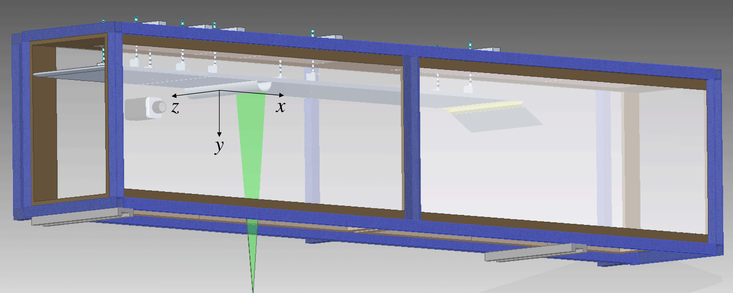
The experiments were conducted in the closed-loop, low-speed wind-tunnel with a 4 m long and $0.75\times 0.5~\text{m}^{2}$ (height and width respectively) cross-sectional area test section (Lindgren & Johansson Reference Lindgren and Johansson2002) at the KTH Fluid Physics laboratory and consisted of a turbulent boundary layer developing on a flat plate, approaching and flowing over a cylindrical bump attached to the plate, as can be seen in figure 1. The 2 cm thick and 3 m long Plexiglas flat plate was placed upside down, i.e. the bump was fixed on the bottom wall of the plate, and fixed 0.13 m beneath the roof of the top section. Although this configuration was necessary as the particle image velocimetry (PIV) laser accessed the test section through the test section bottom wall, all results are presented with the wall-normal axis ( $y$ ) directed towards the top of the page to ease the understanding of the reader. The elliptical leading edge of the flat plate was tripped using two arrays of DYMO tape with the letter ‘V’ embossed in order to trigger the boundary layer transition. The windward edge of the cylindrical bump is placed 1 m downstream of the leading edge of the plate and occupies the entire span of the test section (of 0.5 m span). The diameter of the cylinder is $D=2h=0.100\pm 0.005~\text{m}$ and the distance in the wall-normal direction from the plate to the test section wall is equal to 0.6 m giving a blockage ratio of 9 %. Thin, transparent end plates were mounted on the plate, with an insert for the bump, expanding from $1D$ upstream of the cylinder to $4D$ downstream and over $3D$ in the wall-normal direction, reducing the effective spanwise length to $L=0.4~\text{m}$ and the aspect ratio of the bump to $L/h=8$ . The end plates were needed to reduce the controlled spanwise length as the number of actuators to be applied on the bump was limited by the power source. In the following $x$ is the coordinate in the streamwise direction, $y$ is normal to the flat plate and $z$ is in the spanwise direction. The origin of the coordinate system is at the cylinder centre (1.05 m from the plate leading edge) and on the centreline of the plate.

Figure 1.

Drawing of the set-up with the plate and cylindrical bump mounted upside down and attached to the top wall of the test section. The green area represents the laser sheet used for the PIV measurements and the camera can be seen placed behind the test section from the viewer’s point of view. This PIV configuration was used for PIV measurements in the streamwise/wall-normal plane ( $xy$ -plane). Flow is from left to right.

Figure 2.

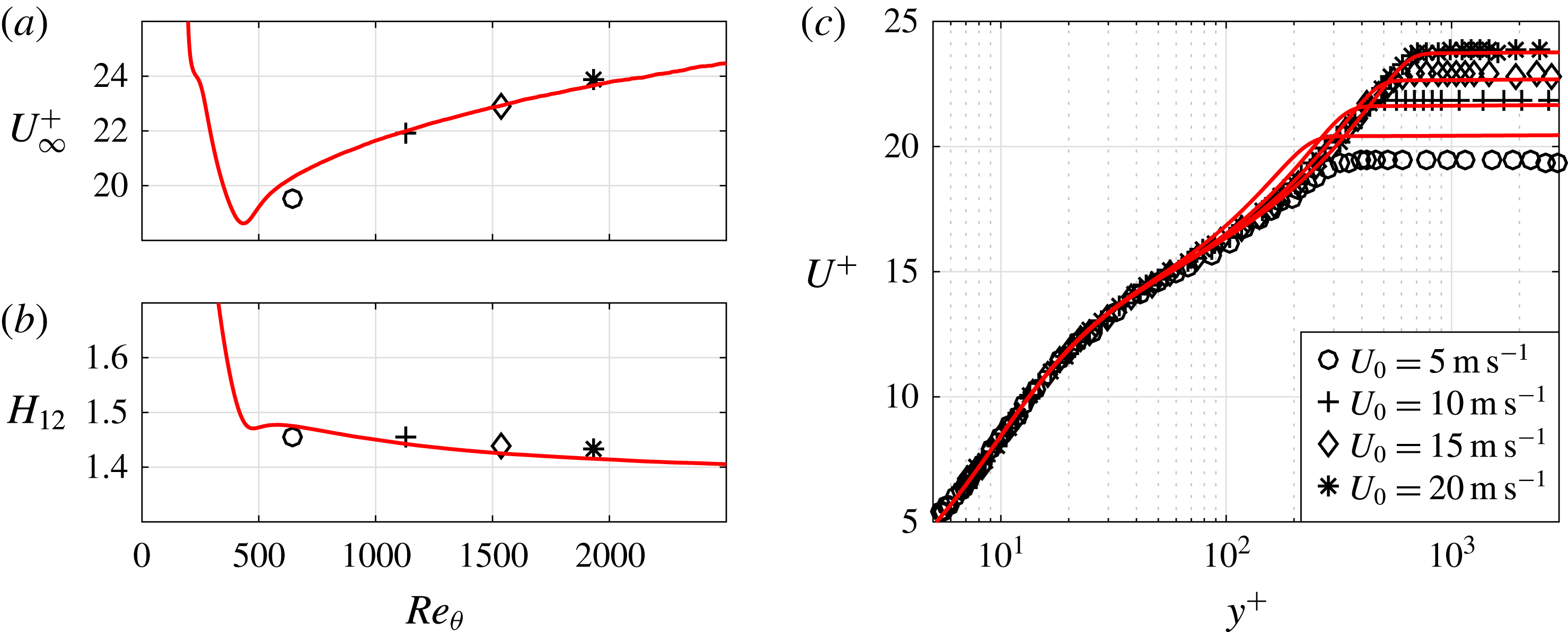
Characteristics of the incoming turbulent boundary layer for $U_{0}=5$ , 10, 15 and $20~\text{m}~\text{s}^{-1}$ . (a) Inner-scaled free-stream velocity, i.e.  $U_{\infty }^{+}$ , and (b) shape factor $H_{12}$ as a function of momentum-loss thickness based Reynolds number $Re_{\unicode[STIX]{x1D703}}$ , as well as (c) inner-scaled mean streamwise velocity together with results from DNS (solid lines) of a zero-pressure-gradient turbulent boundary layer (Schlatter & Örlü Reference Schlatter and Örlü2010) at matched  $Re_{\unicode[STIX]{x1D703}}$ .

The inlet velocity $U_{0}$ was set using a Prandtl tube placed at the inlet of the test section and monitored with a pressure transducer of type Furness FC012, variations of the inlet velocity were observed to be lower than 1 %. The measurements were realised for different inlet velocities $U_{0}$ of 5, 10, 15 and $20~\text{m}~\text{s}^{-1}$ resulting in a range of Reynolds numbers based on $U_{0}$ and the height ( $h$ ) of the cylinder from $Re_{h}=17\times 10^{3}$ to $Re_{h}=67\times 10^{3}$ .

Prior to the flow control study, the flat-plate configuration, i.e. without the bump, was used for the study of the streamwise vortices created by the DBD plasma actuators; the trailing edge of the actuators was placed 0.6 m downstream of the flat-plate leading edge. Figure 2 shows some turbulent boundary characteristics at a position 0.6 m downstream of the leading edge for the four inlet velocities of this study. These measurements were done with hot-wire anemometry and without the cylindrical bump mounted.

The ratio $U_{\infty }^{+}=U_{\infty }/u_{\unicode[STIX]{x1D70F}}$ , where $U_{\infty }$ is the local free-stream velocity and $u_{\unicode[STIX]{x1D70F}}$ is the friction velocity, and the shape factor $H_{12}$ are plotted as function of the Reynolds number based on the momentum-loss thickness ( $\unicode[STIX]{x1D703}$ ). The present results are compared with direct numerical simulation (DNS) results from Schlatter & Örlü (Reference Schlatter and Örlü2010). As can be seen there is an overall good agreement which gives confidence that the tripping is efficient enough so that the boundary layer can be viewed as fully turbulent also at the lowest Reynolds number (cf.  Schlatter & Örlü Reference Schlatter and Örlü2012). Furthermore figure 2(c) shows the mean velocity distribution in the direction normal to the plate ( $y$ ) in the standard logarithmic–linear plot and also here there is a good agreement between the DNS results and the present experiments. Besides using these hot-wire measurements to assess the incoming turbulent boundary layer to the bump, the data were also used to design the DBD-VGs as will be discussed in § 2.2. In particular, the boundary layer thickness $\unicode[STIX]{x1D6FF}$ (which is approximately 18, 14, 13 and 12 mm for the 5, 10, 15 and $20~\text{m}~\text{s}^{-1}$ cases, respectively) at the station of the hot-wire measurements is taken as the characteristic length scale for the design.

2.2 DBD-VG plasma actuator

The DBD plasma actuators are in-house built and made of $66~\unicode[STIX]{x03BC}\text{m}$ -thick copper electrodes applied on both sides of a $396~\unicode[STIX]{x03BC}\text{m}$ thick dielectric sheet made of Kapton and Teflon layers. Positioning the electrodes asymmetrically, with a small overlap of 0.5 mm, as advised by Post & Corke (Reference Post and Corke2004), and applying a high-voltage, high-frequency alternating current between the electrodes produces a plasma. As the actuators are placed on a surface, the plasma only develops along the top electrode, also called the exposed electrode, on the side disposed above the bottom electrode, the former being then embedded. The width of the embedded electrode is an important parameter of DBD plasma actuators as a too narrow electrode would limit the extension of the plasma (Enloe et al. Reference Enloe, McLaughlin, Van Dyken, Kachner, Jumper, Corke, Post and Haddad2004; Forte et al. Reference Forte, Jolibois, Pons, Moreau, Touchard and Cazalens2007). After observing that the plasma extends over only a few millimetres from the edge of the exposed electrode, the bottom electrode width was then chosen to be equal or higher than 10 mm.

To produce CtR streamwise vortices, the DBD-VG plasma actuators were built with the electrodes oriented in the streamwise direction as Jukes & Choi (Reference Jukes and Choi2012) showed that aligning the exposed electrode with the flow direction was optimal for the production of streamwise vortices. An electrode was placed below the dielectric on both sides of the exposed electrode as well as at its extremity, producing a plasma along three sides of the electrode as depicted in figure 3. The actuation length was chosen to be equal to 40 mm ( $\ell$ ) on the sides and 14 mm ( $d$ ) at the extremity of the top electrode. The spacing between the exposed electrodes, i.e. the actuation wavelength, was 55.5 mm ( $\unicode[STIX]{x1D706}$ ). The parameters $\unicode[STIX]{x1D706}$ and $d$ were selected using the boundary layer thickness at $U_{0}=5~\text{m}~\text{s}^{-1}$ (i.e. 18 mm) from the hot-wire measurements shown in figure 2 and parametric studies on passive VGs (Lögdberg, Fransson & Alfredsson Reference Lögdberg, Fransson and Alfredsson2009). The actuation length ( $\ell$ ) was chosen from the literature (among others Jukes & Choi Reference Jukes and Choi2012) and to be able to test driving voltages ( $V_{d}$ ) of up to $12~\text{kV}_{p-p}$ as the available power was limited. In this configuration a total of seven exposed electrodes were used along the spanwise direction giving rise to seven pairs of CtR vortices. For the study of the formation of the streamwise vortices, the actuator and its support were directly mounted on the flat plate creating a 0.83 mm high step protruding from the plate. When applying the actuators on the cylinder, the support and the dielectric sheet were applied all around the cylindrical bump to ensure that nothing was protruding from the surface except for the exposed electrodes of the actuator. It should be noted that there are a number of recent studies following the work by Wicks et al. (Reference Wicks, Thomas, Schatzman, Bowles, Corke, Patel and Cain2012), namely Wicks et al. (Reference Wicks, Thomas, Corke, Patel and Cain2015) and Kelley et al. (Reference Kelley, Corke, Thomas, Patel and Cain2016), which investigated the vorticity generation by DBD-VG plasma actuators with respect to the geometrical parameters of the actuator array.

A high-voltage generator of type Minipuls2 (GBS Elektronik) was used to provide the high-voltage, high-frequency, alternating current to the exposed electrode of the DBD plasma actuators while the bottom electrodes were grounded. A high-voltage probe (Pintek Electronics HVP-39PRO) connected to an oscilloscope (Tektronix TDS 2014C) was used to monitor the sine-like wave amplitude and frequency between the Minipuls2 and the exposed electrode of the actuator. The peak-to-peak value of the driving voltage ( $V_{d}$ ) was here varied between 8 and $12~\text{kV}_{p-p}$ and the driving frequency ( $f_{d}$ ) was kept constant and equal to 6.5 kHz.

Figure 3.

Picture of an operated DBD plasma actuator array placed on the flat plate. $\ell =40~\text{mm}$ , $d=14~\text{mm}$ and $\unicode[STIX]{x1D706}=55.5~\text{mm}$ indicate the actuation length, the width of the electrode as well as the centreline spacing between the electrodes (actuation wavelength), respectively. Flow is from left to right.

2.3 Particle image velocimetry measurements

Particle image velocimetry measurements were conducted in order to:

1. (i) characterise the streamwise vortices produced by the DBD-VG plasma actuator in a turbulent boundary layer on the flat plate,

2. (ii) characterise the flow field around the bump for the baseline case, i.e. the uncontrolled case and

3. (iii) study the effect of DBD-VG plasma actuation on the recirculation region downstream of the bump.

In this paper, stereoscopic PIV (S-PIV) data in $yz$ -planes have been used to investigate (i) and 2-D PIV in $xy$ -planes as well as S-PIV in $yz$ -planes were used for (ii) and (iii).

A Dantec Dynamics PIV system was used to conduct the measurements. A Litron Dualpower 50-200 (50 mJ, 200 Hz) Nd:YAG laser produced a laser sheet (approximately 1 mm thick for the 2-D PIV and 2 mm thick for the S-PIV) illuminating an area of approximately $0.2\times 0.2~\text{m}^{2}$ in the plane of interest. Two 12-bit SpeedSense M120 CMOS cameras with a sensor resolution of 1920 $\times$ 1200 pixels and a storage capacity of 1825 image pairs were used to capture images of Diethylhexylsebacate particles of $1~\unicode[STIX]{x03BC}\text{m}$ nominal diameter, produced by a seeding generator (Dantec Dynamics, 10F03 High Volume Liquid Seeder) illuminated by the laser sheet. For the 2-D PIV measurements one camera was employed and was mounted with the optical axis perpendicular to the laser sheet. For the S-PIV a second camera was added to the system in order to be able to reconstruct the third component of the velocity field in the common field of view (FOV) of the two cameras. The cameras were mounted on each side of the test section and separated by an angle of $86^{\circ }$ for the measurements of the streamwise vortices produced by the DBD-VG plasma actuator on the flat plate and $85.5^{\circ }$ for the measurements of the separated flow downstream of the cylindrical bump, hence close to the optimal $90^{\circ }$ .

Figure 4.

Streamwise vortices produced by DBD-VGs for the case with $U_{0}=5~\text{m}~\text{s}^{-1}$ . The colour scale represents the streamwise component of the velocity normalised by $U_{0}$ and the arrows indicate the in-plane motion. The dielectric of the actuator is represented by dark grey, the brown rectangles are the electrodes and the violet part the induced plasma. Flow is from left to right. In the flat-plate configuration $x=0~\text{m}$ is 0.6 m downstream of the leading edge of the flat plate.

Both for 2-D PIV and S-PIV measurements the cameras and the laser were mounted on a traversing system (ISEL C142-4) allowing them to move together in the spanwise and streamwise directions, hence it was possible to change easily the spanwise or streamwise location of the measurement plane. The S-PIV measurements for the study of the vortices produced by the DBD-VGs were carried out at three streamwise locations (0.014, 0.035 and 0.087 m downstream of the edge of the exposed electrodes (as can be appreciated in the three-dimensional figure 4). For the separation control study, successive 2-D PIV measurement planes were recorded along the streamwise direction to reconstruct the entire region of separated flow as well as several successive planes in the spanwise direction to study the effect of the three-dimensional actuation technique (DBD-VGs); a table summarising all 2-D PIV measurements is available as supplementary material available at https://doi.org/10.1017/jfm.2017.773. S-PIV measurements were carried out at the streamwise position $x=0.099~\text{m}$ ( $1.98h$ ) and $x=0.189~\text{m}$ (3.78 $h$ ) as can be seen in figure 5. Moreover, the cameras were mounted on a specific holding system allowing us to rotate the camera, i.e. the image plane, but keep the lens fixed so the Scheimpflug criterion could be fulfilled and the area of focus increased.

The software DynamicStudio v4.10 was used to run the acquisition and the processing of the PIV images. An in situ planar target was used to calibrate the cameras. For the calibration of the S-PIV measurements along the third dimension, hence the streamwise direction in this study, the planar target was kept still inside the test section and the cameras were moved along the streamwise direction using the ISEL traverse to capture the calibration images and a pinhole model was selected. Finally, a calibration refinement was realised on the raw PIV images to correct eventual misalignment errors. The temporal minimum background was removed from the raw PIV images in order to remove noise from the images. The velocity-vector field was evaluated using a multipass iteration procedure starting with an interrogation window size of 64 $\times$ 64 pixels and finishing with 16 $\times$ 16 pixels and 50 % overlap. Finally the ‘universal outlier detection’ (Westerweel & Scarano Reference Westerweel and Scarano2005) was used to detect eventual spurious vectors and replace them by the median value evaluated from 5 $\times$ 5 neighbouring vectors. For 2-D PIV measurements approximately 2 % of spurious vectors were detected and the measurement uncertainty was estimated to be of the order of 0.1 pixel (Raffel et al. Reference Raffel, Willert, Wereley and Kompenhans2007) which represents $0.062~\text{m}~\text{s}^{-1}$ for the measurements with $U_{0}=5~\text{m}~\text{s}^{-1}$ , hence 1.24 % of the inlet velocity.

For the S-PIV measurements, special care has been taken to estimate the vector field as the out-of-plane component of the velocity (streamwise component) was larger in magnitude than the in-plane components. S-PIV measurements were only carried out for inlet velocities $U_{0}$ up to $15~\text{m}~\text{s}^{-1}$ , since for higher velocities the necessary time interval to obtain a good correlation was too short for the current measurement system. During the analysis procedure a minimal value of 10 particles per window of interrogation was imposed on the multipass iteration, hence the iteration procedure started with the largest interrogation size (here 64 $\times$ 64 pixels) and adapted the size of the window for the next pass depending on the number of particles. Finally, in the last step, the vector grid was interpolated on a regular grid with the spacing defined by the last step of the iteration procedure. The spatial resolution of the S-PIV measurements was between 32 pixels and 8 pixels, changing for different regions of the FOV and hence limiting to the measurements and observations of large-scale structures. This method improved the evaluation of the vector field as the number of outliers recognised by the ‘universal outlier detection’ and replaced by the median value decreased to 6 %, while it was higher than 15 % without adapting the interrogation window size to the number of particles.

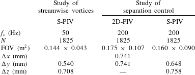
Table 1 summarises the different parameters of the PIV measurements presented here, such as the sampling frequency $f_{s}$ , the number of image pairs recorded $N$ , the size of the FOV and the vector spacing $\unicode[STIX]{x0394}x$ , $\unicode[STIX]{x0394}y$ and $\unicode[STIX]{x0394}z$ . The vector fields were then exported and further analysed in MATLAB (MathWorks).

Figure 5.

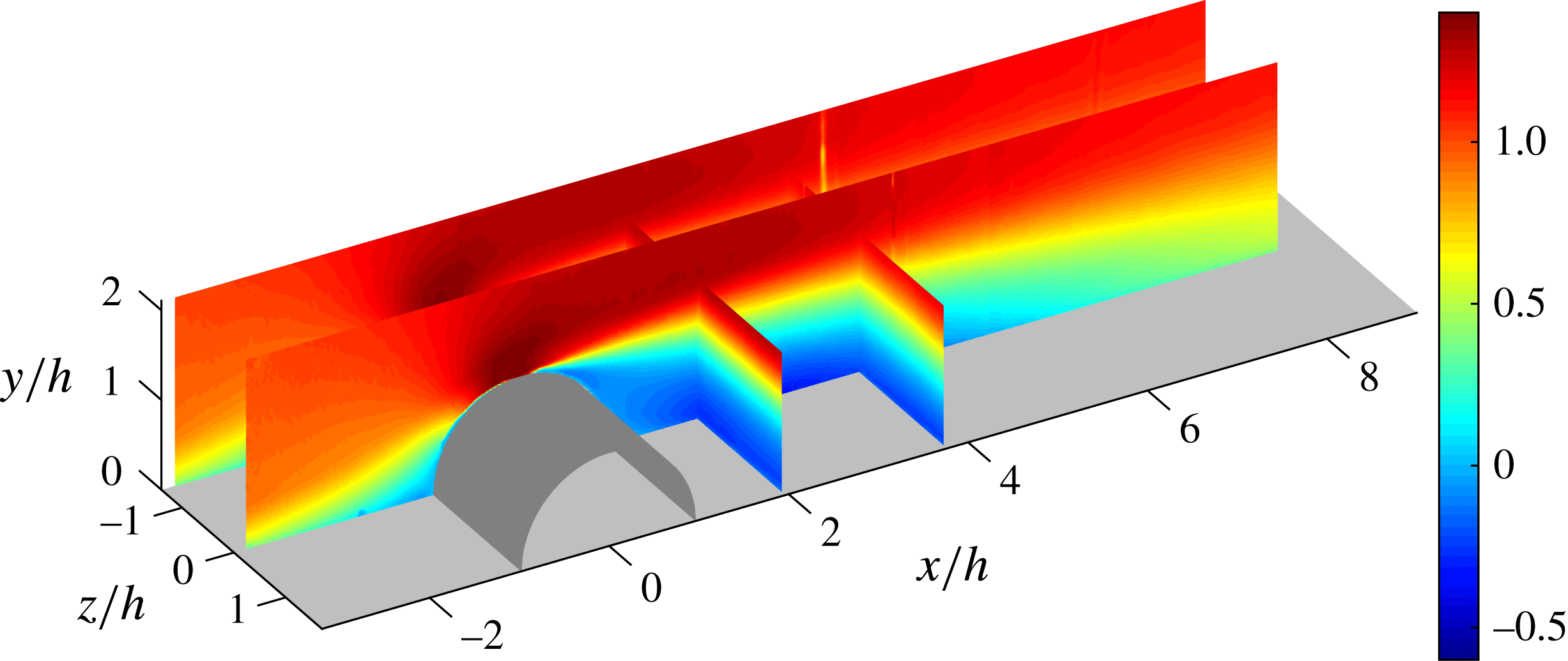
Baseline flow for the case $U_{0}=10~\text{m}~\text{s}^{-1}$ . The colour scale represents the mean streamwise component of the velocity normalised by $U_{0}$ . The flow in the $xy$ -plane is reconstructed from four 2-D PIV measurements. The 2-D PIV at $z/h=0$ and $z/h=-1.388$ . S-PIV in the $yz$ -planes at the positions $x/h=1.98$ and $x/h=3.78$ are also presented. Flow is from left to right.

Table 1.

Parameters and characteristics of the PIV measurements. The dimensions of the FOV correspond to dimension in the spanwise and wall-normal direction, respectively, for the S-PIV measurements and in the streamwise and wall-normal direction, respectively, for the 2-D PIV measurements.

4.1 Baseline flow

The turbulent boundary layer develops upstream of the cylindrical bump and the flow is accelerated as it passes the windward side of the bump under a favourable pressure gradient (FPG). Downstream of the apex of the obstacle, the flow close to the surface of the cylinder loses kinetic energy until it cannot withstand the adverse pressure gradient (APG) and separates; the flow closest to the surface is pressure driven and evolves in the opposite direction to the free-stream flow creating a recirculation region downstream of the cylinder. As Simpson (Reference Simpson1989) described, the curvature also impact the flow separation, the streamlines of the flow not being able to follow strong geometry changes, the detachment of the flow is also a consequence of mass conservation. Once the pressure gradient decreases and relaxes to zero, the flow recovers and reattaches to the flat plate, closing the recirculation region as is apparent from figure 5.

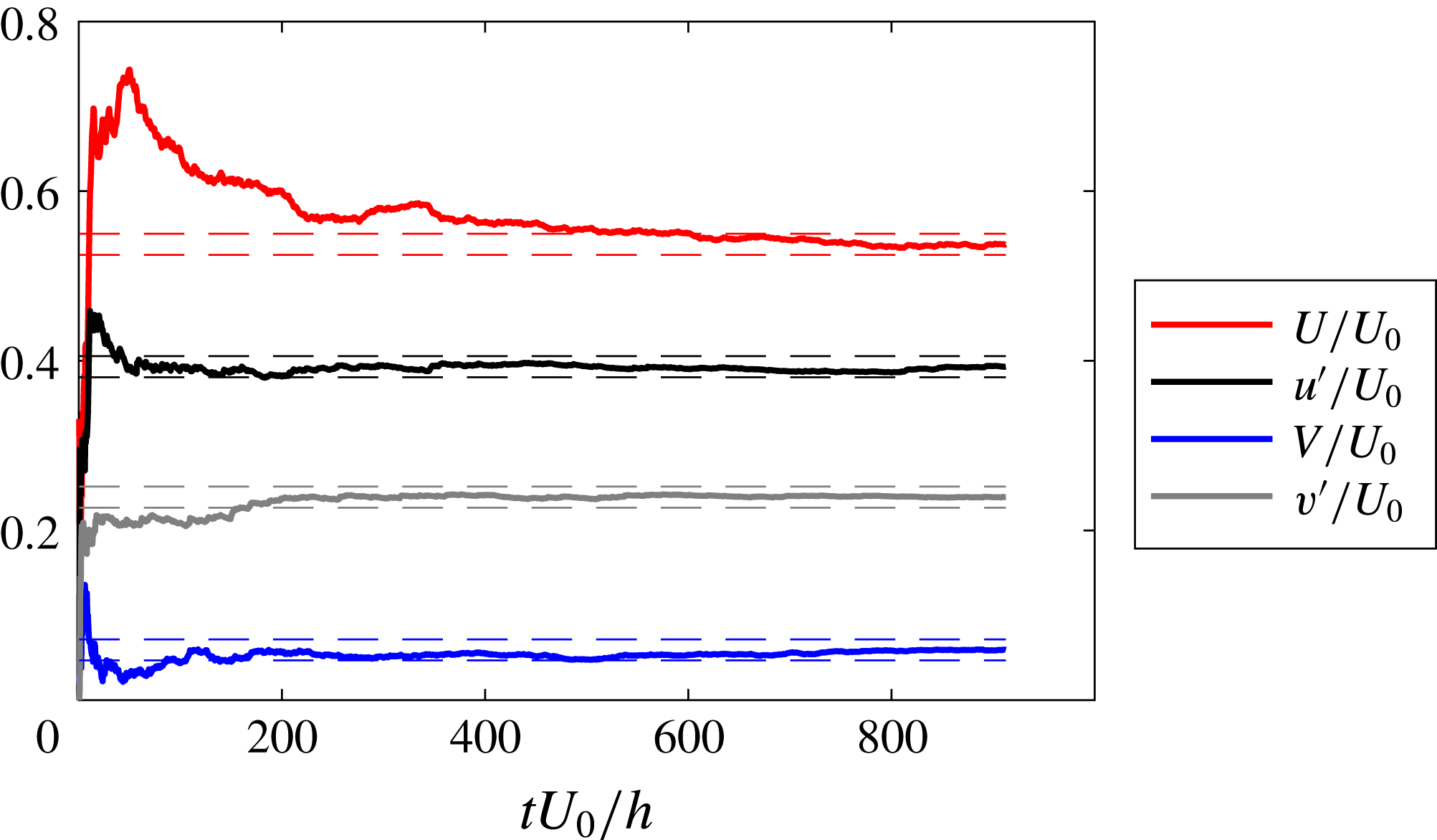
Since the field of interest in the $xy$ -plane is larger than the field of view of the PIV camera, 4 planes were stacked together thereby spanning an area of $11.5h\times 2.2h$ (length $\times$ height). Figure 5 also shows spanwise/wall-normal planes, indicating the spanwise homogeneity of the mean flow. Since the flow field shown in figure 5 consists of several independent experimental views, statistical convergence needs to be ensured prior to combining the different FOVs. Therefore, a convergence study was conducted for the flow case at $U_{0}=5~\text{m}~\text{s}^{-1}$ , which constitutes the most crucial one in terms of the eddy-turnover time. As apparent from figure 6 the streamwise and wall-normal mean and r.m.s. components are well converged for the lowest free-stream velocity, thereby ensuring that the cases at higher $U_{0}$ are at least equally well converged.

Figure 6.

Statistical convergence for the measurements at $U_{0}=5~\text{m}~\text{s}^{-1}$ without actuation. The study is conducted in the shear layer at $x/h=0.4$ and the wall-normal position corresponding to the maximum streamwise r.m.s. value. The bounds correspond to the estimated measurement uncertainty of the PIV measurements i.e.  $\pm$ 0.0124 for this case.

4.2 Effect of control on the recirculation area

In this section the effect of actuation with the DBD-VG plasma actuator on the recirculation region is investigated. A measure of this effect is how the length of the recirculation region changes with actuation. Therefore, the position of the reattachment point of the boundary layer downstream of the bump is evaluated for the different measurement cases in order to quantify this effect. Simpson (Reference Simpson1989) defines various stages of flow detachment. He defines incipient detachment as the location where the flow is directed in the opposite direction as compared to the free-stream direction, i.e. backflow, 1 % of the time, intermittent transitory detachment where backflow occurs 20 % of the time and transitory detachment where backflow occurs 50 % of the time. He also defines detachment where the mean wall-shear stress is equal to zero. In general, transitory detachment and detachment occur close to each other, but not necessarily at exactly the same streamwise position. In principle the direction of the flow should be determined by the wall-shear stress, but since the sign of $u$ and $\text{d}u/\text{d}y$ is the same close to the wall, the velocity there can be used as a measure of backflow. The definition of Simpson (Reference Simpson1989) can be extended to find the reattachment location as the location where the flow is directed in the backflow direction 50 % of the time. In the experiments we do not have the possibility to measure the wall-shear stress directly and therefore we investigate the PIV measurements to find the flow direction at a position close to the wall to determine the backflow coefficient $\unicode[STIX]{x1D712}$ , i.e. the amount of time (with respect to the total time) the flow spends in the upstream direction, and the location of shear-layer reattachment $x_{\unicode[STIX]{x1D712}=50}$ (as commonly done in the literature, e.g. Angele & Muhammad-Klingmann Reference Angele and Muhammad-Klingmann2006; Lögdberg, Angele & Alfredsson Reference Lögdberg, Angele and Alfredsson2008).

Figure 7 shows the evolution of $\unicode[STIX]{x1D712}$ downstream of the cylindrical bump for the different inlet velocities (i.e.  $U_{0}=5$ , 10, 15 and $20~\text{m}~\text{s}^{-1}$ ). The PIV data from $xy$ -plane measurements close to the wall ( ${<}1~\text{mm}$ from the wall) are used to evaluate $\unicode[STIX]{x1D712}$ and the horizontal red line represents $\unicode[STIX]{x1D712}=50\,\%$ to help evaluate at which $x$ -position the flow is considered as separated or attached to the plate. The measurements are realised along the centreline of the test section ( $z/h=0$ ) for the cases at $U_{0}=5$ and $10~\text{m}~\text{s}^{-1}$ and at $z/h=-0.278$ for the cases at 15 and $20~\text{m}~\text{s}^{-1}$ . Immediately downstream of the cylinder, the flow is attached to the plate as $\unicode[STIX]{x1D712}<50\,\%$ for all inlet velocities; this is due to the presence of a small recirculation region forming at the corner between the downstream side of the bump and the plate and rotating in the opposite direction to the main recirculation region, i.e. in the anti-clockwise direction (cf. figure 5). For simplicity, here and henceforth, reattachment and separation are taken as those locations where $\unicode[STIX]{x1D712}=50\,\%$ , which coincides with the skin-friction coefficient being equal to zero, as found in Alving & Fernholz (Reference Alving and Fernholz1995) and employed in recent studies (Angele & Muhammad-Klingmann Reference Angele and Muhammad-Klingmann2006; Lögdberg et al. Reference Lögdberg, Angele and Alfredsson2008). The curves present some outliers around the position $x/h=4.1$ ; this is an error caused by a distortion of the PIV laser sheet when passing through a joint in the test section window. The decreasing rate of $\unicode[STIX]{x1D712}$ is different depending on the inlet velocity, when $U_{0}$ increases, and the reattachment position ( $x_{\unicode[STIX]{x1D712}=50}$ ) moves upstream showing that the Reynolds number has an effect on the length of the recirculation bubble, as can be seen in figure 7 and was previously shown by the authors in Vernet, Örlü & Alfredsson (Reference Vernet, Örlü, Alfredsson, Peinke, Kampers, Oberlack, Waclawczyk and Talamelli2016); the higher the Reynolds number, the shorter the recirculation region.

Figure 7.

Evolution of the percentage of backflow $\unicode[STIX]{x1D712}$ close to the wall and along the streamwise direction $x$ for the baseline flow. The horizontal red line indicates $\unicode[STIX]{x1D712}=50\,\%$ .

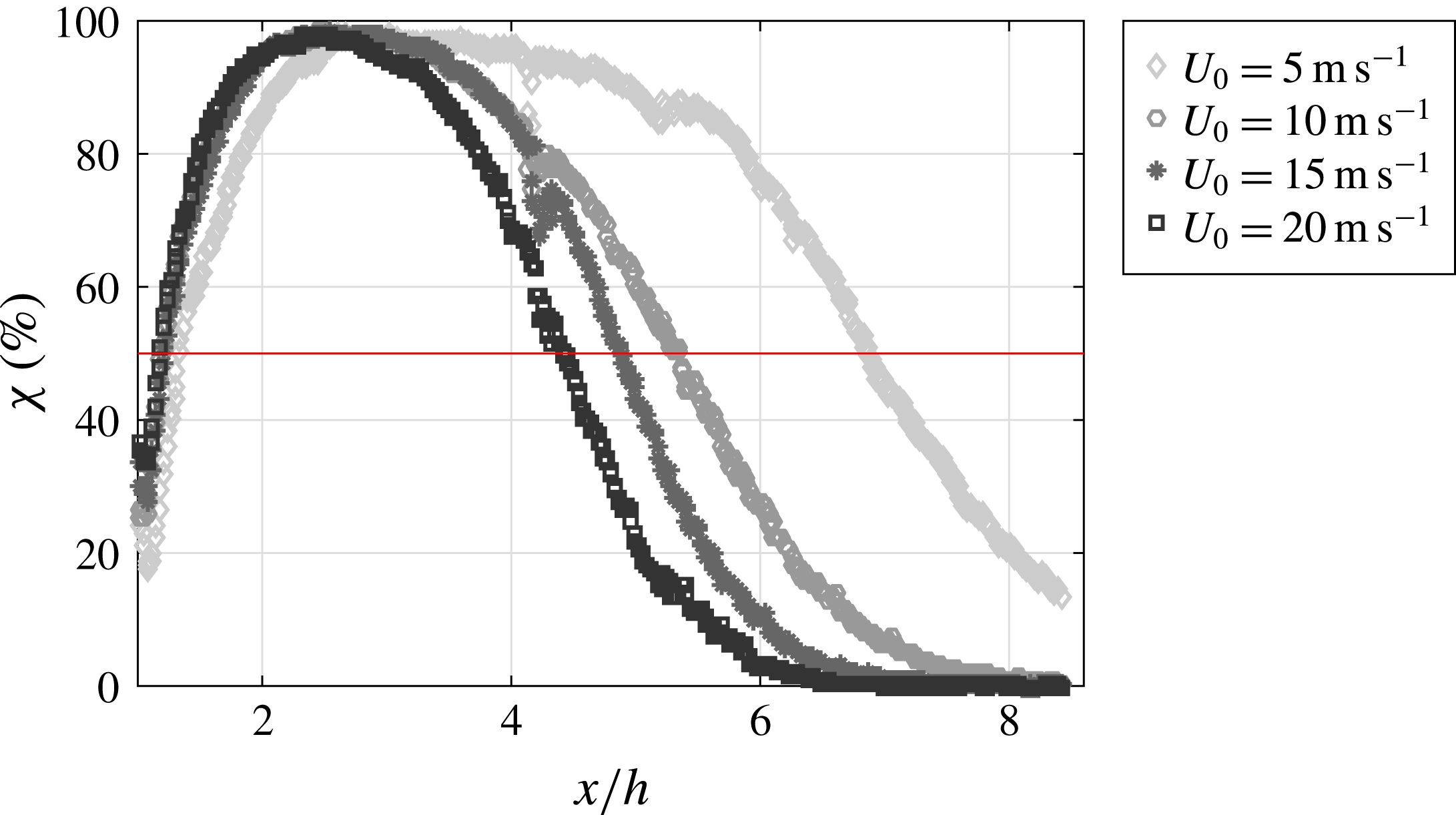
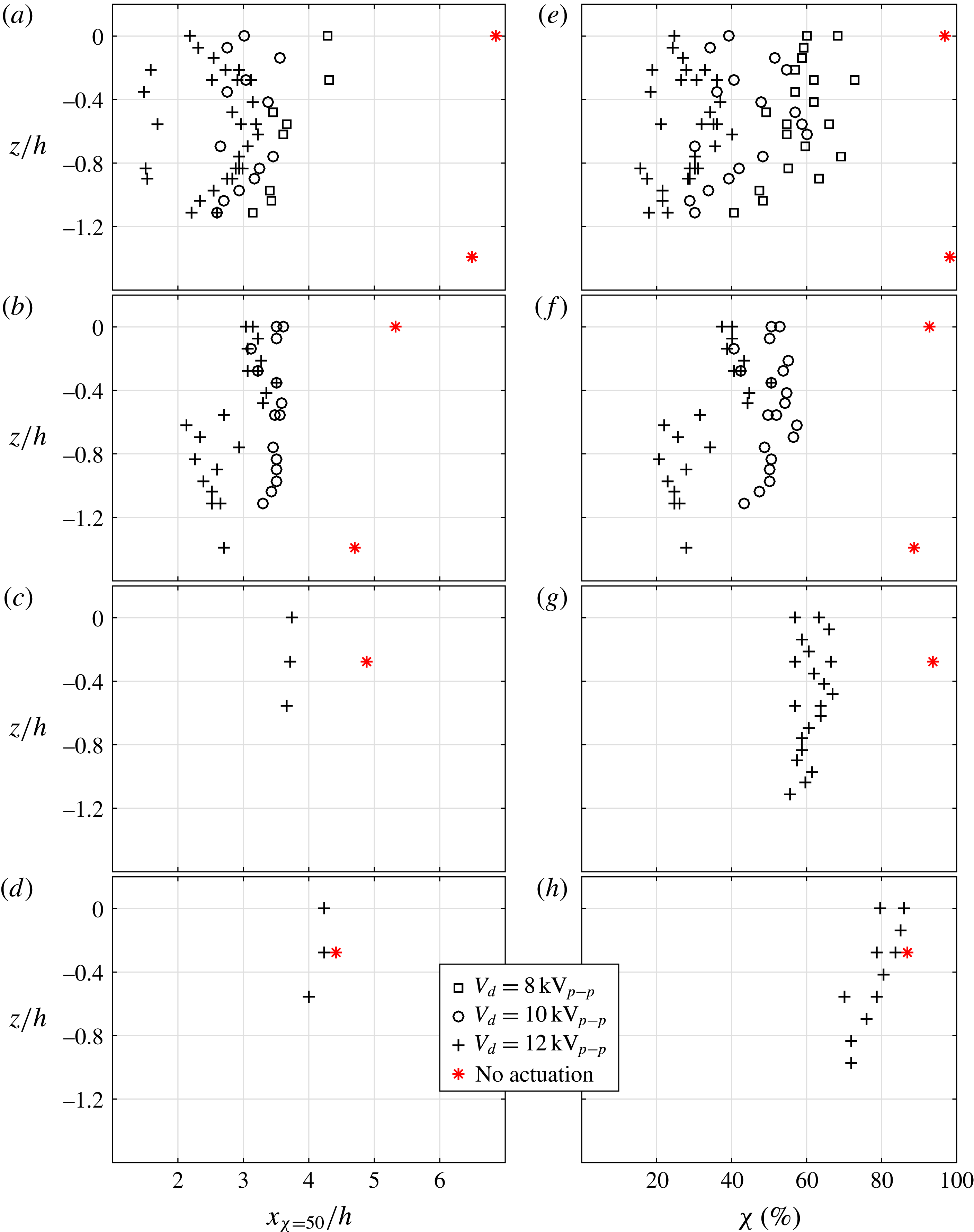
Figure 8(a,c,e,g), the streamwise location of the flow reattachment ( $x_{\unicode[STIX]{x1D712}=50}$ ) is compared between cases with and without actuation for all inlet velocities $U_{0}$ tested. The red marks show the location of the reattachment for the baseline case while the black marks correspond to the cases with the DBD-VG plasma actuator activated; different symbols are used for the different driving voltages $V_{d}$ tested.

Figure 8.

Streamwise location of the flow reattachment $x_{\unicode[STIX]{x1D712}=50}/h$ (a–d) and percentage of backflow $\unicode[STIX]{x1D712}$ at $x/h=3.5$ (e–h) at different $z/h$ and close to the wall, with and without actuation, for $U_{0}=5~\text{m}~\text{s}^{-1}$ (a,e), $10~\text{m}~\text{s}^{-1}$ (b,f), $15~\text{m}~\text{s}^{-1}$ (c,g) and $20~\text{m}~\text{s}^{-1}$ (d,h).

For the cases at $U_{0}=5$ and $10~\text{m}~\text{s}^{-1}$ , shown in figure 8(a,b), the baseline flow was studied at two different spanwise locations and it can be observed that the recirculation region is slightly longer in the centre of the test section than closer to the side walls, which could be due to an influence of the side walls. As shown by Tylli, Kaiktsis & Ineichen (Reference Tylli, Kaiktsis and Ineichen2002), studying side-wall effects in flows over backward-facing steps, the secondary flow away from the side-walls results in the development of wall-jet profiles, which causes flow three-dimensionality. However, this is found to be a noticeable only for high Reynolds number laminar and transitional flows. Furthermore, the length of the recirculation region seems to be strongly influenced by the DBD-VG plasma actuation for cases with $U_{0}$ up to $15~\text{m}~\text{s}^{-1}$ . Figure 8(a) shows that for $U_{0}=5~\text{m}~\text{s}^{-1}$ and $z/h=0$ , $x_{\unicode[STIX]{x1D712}=50}$ moves 2.6 $h$ upstream when using a driving voltage of $8~\text{kV}_{p-p}$ , 3.9 $h$ with $V_{d}=10~\text{kV}_{p-p}$ and 4.7 $h$ with $V_{d}=12~\text{kV}_{p-p}$ . These results seem to indicate that a higher driving voltage induces a stronger control effect and a larger reduction of the recirculation region, as also shown for the case with $U_{0}=10~\text{m}~\text{s}^{-1}$ shown in figure 8(b).

Most of the 2-D PIV measurements were realised with a FOV extending from $x/h=0.14$ to 3.62 and thus could not show the flow reattachment location if the latter occurred downstream of the FOV. As this could lead to a misinterpretation of the results based on figure 8(a–d), the right panels of the figure, i.e. figure 8(e–h), show the percentage of backflow $\unicode[STIX]{x1D712}$ at the streamwise location $x/h=3.5$ for all measurements available at this location. These plots confirm that the DBD-VG plasma actuators have a strong effect on the length of the recirculation region as $\unicode[STIX]{x1D712}$ becomes smaller when the actuator is activated than for the baseline flow. It also confirms that by increasing the voltage the control effect increases since $\unicode[STIX]{x1D712}$ is reduced for most of the measurements, as is apparent from figure 8(e–g). Ultimately, the ability of the actuators to have a sustained effect on the recirculation bubble seems to vanish for the highest tested velocity, i.e.  $U_{0}=20~\text{m}~\text{s}^{-1}$ .

Another observation that can be made when inspecting figure 8, is the three-dimensionality of the location of the reattachment for the cases with actuation. As expected, the position moves slightly upstream as $z$ decreases, i.e. the measurement plane comes closer to the end walls as compared to the baseline case. Furthermore, the actuation is three-dimensional when using DBD-VG plasma actuators, which could result in a three-dimensional reattachment location. However, in this case $x_{\unicode[STIX]{x1D712}=50}$ should appear periodic along the spanwise direction matching the wavelength of the actuation and should be consistent when repeating measurements in the same conditions. In reality, however, the inhomogeneity of the results do not fit any of the explanations given above and furthermore increases with increasing $V_{d}$ . The next section demonstrates that this is an effect of the flow showing bi-modality under actuation.

5.1 Bi-modality of the flow

A turbulent flow is unsteady by definition and often studied in terms of the statistics of the velocity components, thus the measurement time and frequency must be chosen adequately in order to obtain converged statistics. It was shown in figure 6, that for the sampling time used the random errors became smaller than the measurement uncertainty of the baseline flow with $U_{0}=5~\text{m}~\text{s}^{-1}$ . This is then also true for higher inlet velocities since the sampling time was kept constant for all cases. However, as will be shown below, the flow under actuation exhibits a low-frequency unsteadiness that we denote as an inherent bi-modality, i.e. flow structures change between two rather distinct locations.

We first illustrate this bi-modality by studying time series of the streamwise component of the velocity ( $u$ ). The data are obtained from S-PIV measurements in the spanwise/wall-normal ( $zy$ ) plane at the streamwise position $x/h=1.98$ .

Figure 9 shows the evolution of the spanwise distribution of $u$ with time ( $tU_{0}/h$ ) at $x/h=1.98$ and $y/h=0.6$ above the plate, with $U_{0}=10~\text{m}~\text{s}^{-1}$ . The figure shows three cases: the first case (figure 9 a) is without actuation (baseline case) and then two cases with different strength of actuation; figure 9(b) with $V_{d}=10~\text{kV}_{p-p}$ and figure 9(c) with $V_{d}=12~\text{kV}_{p-p}$ . Black indicates negative (i.e. backflow) and white positive streamwise velocity. As apparent the DBD-VG plasma actuation has a clear effect on the flow and, in particular, introduces large time scales in the flow. The baseline flow shows only high-frequency unsteadiness as inherent in a turbulent flow, while the actuated flow cases seem to be more organised and show a clear low-frequency variation. The ordinate of figure 9 is normalised with the bump height, hence the location of the centre of the electrodes are aligned with $z/h=-1.11$ , 0 and 1.11. The structures developing in case of actuation have a spanwise wavelength close to twice the actuation wavelength, i.e. when $u$ is positive between the spanwise position $z/h=-1.11$ and 0, it is negative between $z/h=0$ and 1.11 and vice versa. This observation seems to indicate that the structure is not directly linked to the streamwise vortices produced by the DBD-VGs actuators as the same flow behaviour would then occur between $z/h=-1.11$ and 0, as well as $z/h=0$ and 1.11. Furthermore, the low-frequency alternation between positive and negative states indicates a bi-modality of the flow.

Figure 9.

Evolution of $u$ along the spanwise direction at $(x/h,y/h)=(1.98,0.6)$ with time for the cases at $U_{0}=10~\text{m}~\text{s}^{-1}$ . Panel (a) shows the case without actuation (baseline flow), while (b) is with an actuation at $V_{d}=10~\text{kV}_{p-p}$ and (c) at $12~\text{kV}_{p-p}$ . Black represents $u<0$ and white $u>0$ .

To be able to further quantify this low-frequency phenomenon, the area of separated flow $A_{0}(t)$ in a domain $\unicode[STIX]{x1D6FA}$ can be defined following Pearson, Goulart & Ganapathisubramani (Reference Pearson, Goulart and Ganapathisubramani2013). For the instantaneous velocity field at time $t$ a measure, $A_{0}(t)$ , is evaluated according to:

This definition is valid for a three-dimensional field, however, since here 2-D PIV and S-PIV are employed and two-dimensional velocity fields are obtained, the domain $\unicode[STIX]{x1D6FA}$ is consequently applied on a two-dimensional domain.

As the spanwise wavelength for the low-frequency phenomenon is close to the span of the FOV of the S-PIV measurements, $A_{0}(t)$ would be constant with time if the whole FOV was taken as $\unicode[STIX]{x1D6FA}$ . Instead, two domains were considered: $\unicode[STIX]{x1D6FA}_{1}$ is defined from the span position $z/h=-1.11$ (i.e.  $z/\unicode[STIX]{x1D706}=-1$ ) to the position $z/h=0$ and covers the entire FOV of the S-PIV in the wall-normal direction. $\unicode[STIX]{x1D6FA}_{2}$ covers the same size wall-normal span as $\unicode[STIX]{x1D6FA}_{1}$ for $z/h=0$ to 1.11 (i.e.  $z/\unicode[STIX]{x1D706}=1$ ).

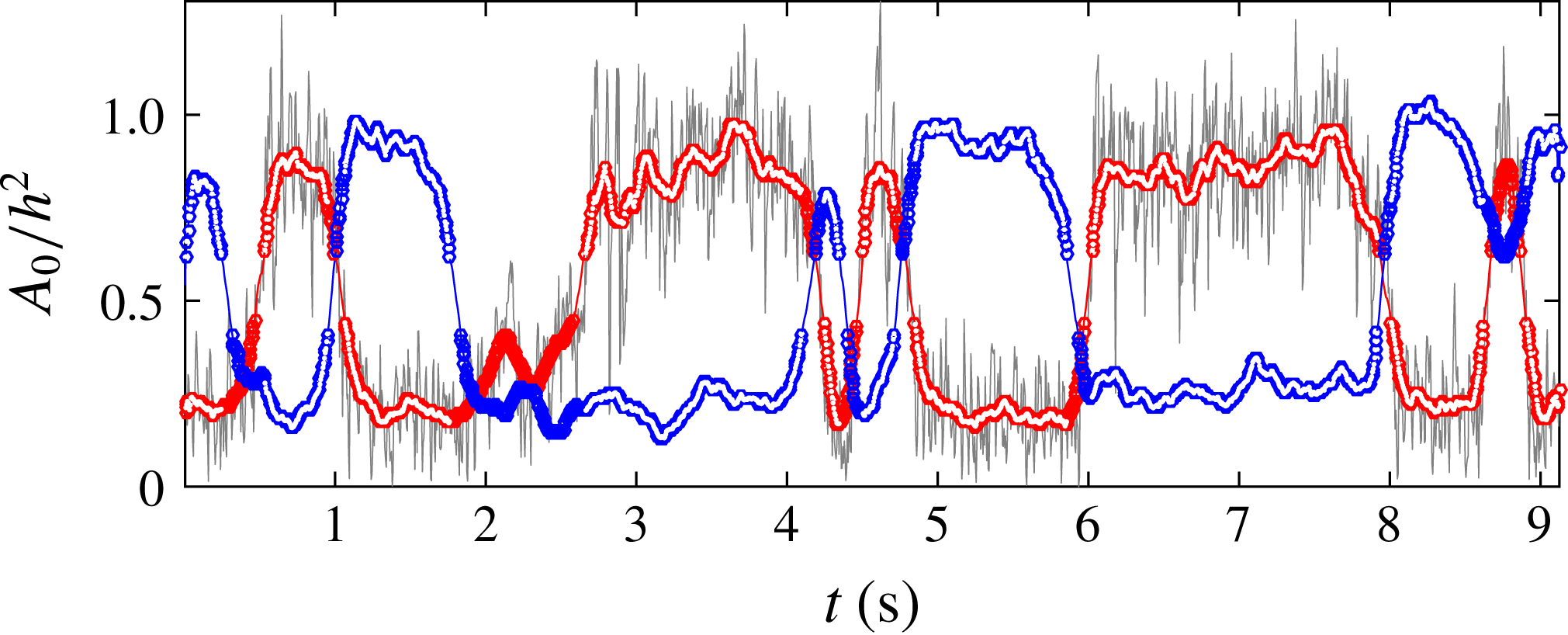
Figure 10 shows the evolution of $A_{0}(t)$ normalised by $h^{2}$ in the domain $\unicode[STIX]{x1D6FA}_{1}$ (grey curve) and can be linked to figure 9(c), i.e. 

1. – when $u$ is positive (white colour), between $z/h=-1.11$ and 0 the normalised area of separated flow $A_{0}/h^{2}$ is low, i.e. approximately 0.25, whereas

2. – when $u$ is negative (black colour), the value of $A_{0}/h^{2}$ is high, i.e. approximately 0.9.

Figure 10.

Evolution of $A_{0}/h^{2}$ in the domain $\unicode[STIX]{x1D6FA}_{1}$ in grey and low-pass filtered $A_{0}/h^{2}$ in $\unicode[STIX]{x1D6FA}_{1}$ in red. The blue curve is the low-pass filtered $A_{0}/h^{2}$ in $\unicode[STIX]{x1D6FA}_{2}$ . The fully blue and red symbols denote data which are evaluated to be part of the same flow mode. The symbols filled in white show the data used in the conditional averaging.

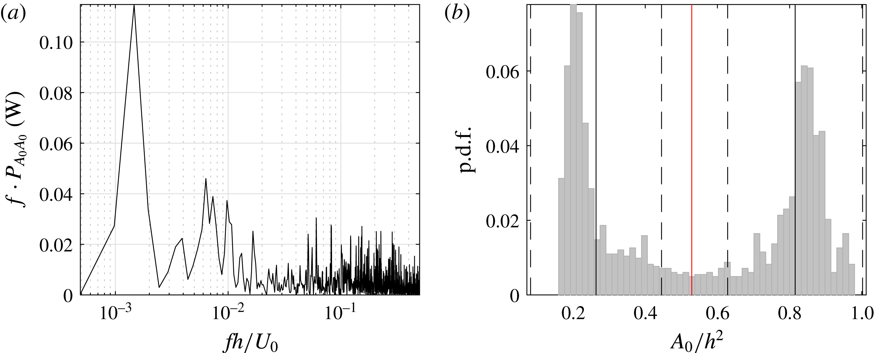
The spectra of the time evolution of the area of separated flow $A_{0}$ in $\unicode[STIX]{x1D6FA}_{1}$ , given in figure 11(a), confirms the dominance of low-frequency variations with a value of around $fh/U_{0}=0.0015$ . As the bi-modality is linked to this low frequency, a low-pass filter at $fh/U_{0}=0.025$ is applied to the signal of $A_{0}$ ; the low-pass filtered $A_{0}/h^{2}$ in $\unicode[STIX]{x1D6FA}_{1}$ corresponds to the red curve in figure 10, while the low-pass filtered $A_{0}/h^{2}$ in $\unicode[STIX]{x1D6FA}_{2}$ corresponds to the blue curve. These two signals, which are expectedly anti-correlated, confirm that the wavelength of the structure developing in the flow is close to double the actuation wavelength as was observed in figure 9.

Figure 11.

(a) Premultiplied spectra of $A_{0}$ in $\unicode[STIX]{x1D6FA}_{1}$ . (b) Probability density function (p.d.f.) of the low-pass filtered $A_{0}/h^{2}$ in grey; the red line is the separation line between the two states of the bi-modal p.d.f. evaluated using the Otsu thresholding method, while the full black lines indicate the mean ( $\unicode[STIX]{x1D707}$ ) of each of the two states and the dashed lines indicate the range $\unicode[STIX]{x1D707}\pm 2\unicode[STIX]{x1D70E}$ of each state.

The low-pass filtered $A_{0}/h^{2}$ in $\unicode[STIX]{x1D6FA}_{1}$ and $\unicode[STIX]{x1D6FA}_{2}$ evolve between a low and a high state (see figure 10). This is also visible in figure 11(b) showing the probability density function (p.d.f.) of the low-pass filtered signal $A_{0}/h^{2}$ in $\unicode[STIX]{x1D6FA}_{1}$ . The bi-modality of the p.d.f. highlights these two states. The Otsu thresholding method (Otsu Reference Otsu1979) commonly used for image grey-level segmentation is used here to separate the two states or classes. The method uses the histogram to find the threshold value between the two classes corresponding to the minimum of the within-class variance, also called the intra-class variance. For this case, the Otsu method gives a threshold of the bi-modal p.d.f. at $A_{0}/h^{2}=0.53$ ; this value is represented by the vertical red line in figure 11(b). Each state of the bi-modal p.d.f. is then analysed independently, i.e. their mean ( $\unicode[STIX]{x1D707}$ ), represented by the full black lines, and their standard deviation ( $\unicode[STIX]{x1D70E}$ ) is calculated. Values inside the range of $\unicode[STIX]{x1D707}\pm 2\unicode[STIX]{x1D70E}$ for each state (dashed lines in figure 11 b) are selected to be part of a conditional averaging; these values are presented with red symbols in figure 10. A first conditional average will represent data for which $A_{0}/h^{2}$ is in the low state (low values, i.e. left side of the bi-modal p.d.f.) and a second conditional average will use data in the high state (high values, i.e. right side of the p.d.f.).

The same method is applied to the low-pass filtered signal $A_{0}/h^{2}$ in $\unicode[STIX]{x1D6FA}_{2}$ and the values selected to be part of the conditional averages are represented by blue symbols. As mentioned, the two signals are anti-correlated except during short transition periods. To avoid utilising these instances, the conditional-averaging operation is limited to data present in the low state in $\unicode[STIX]{x1D6FA}_{1}$ while simultaneously in the high state in $\unicode[STIX]{x1D6FA}_{2}$ and vice versa. The data fulfilling this additional condition are represented by white dots in figure 10. To summarise, the two conditional averages or modes are defined as:

1. – Mode A: $A_{0}/h^{2}$ in $\unicode[STIX]{x1D6FA}_{1}$ is in the low state while $A_{0}/h^{2}$ in $\unicode[STIX]{x1D6FA}_{2}$ is in the high state (yielding 578 instantaneous velocity fields, corresponding to 32 % of the total measurement data) and,

2. – Mode B: $A_{0}/h^{2}$ in $\unicode[STIX]{x1D6FA}_{1}$ is in the high state while $A_{0}/h^{2}$ in $\unicode[STIX]{x1D6FA}_{2}$ is in the low state (yielding 792 instantaneous velocity fields, corresponding to 43 % of the total measurement data).

Contour plots of the two modes are depicted in figure 12(b,c), while figure 12(a) shows the mean using the complete dataset.

Figure 12.

Averages of the instantaneous velocity fields of the S-PIV measurement at $x/h=1.98$ ( $U_{0}=10~\text{m}~\text{s}^{-1}$ , $V_{d}=12~\text{kV}_{p-p}$ ). (a) Mean based on the full dataset (1825 instantaneous fields), (b) conditional averaging of mode A (578 instantaneous fields), (c) conditional averaging of mode B (792 instantaneous fields). The colour scale represents the streamwise component of the velocity normalised by $U_{0}$ and the arrows the in-plane motion. White vectors indicate the strongest in-plane velocity vector corresponding to (a) 0.25, (b) 0.57 and (c) 0.54 $U_{0}$ .

The conditionally averaged data in figure 12(b,c) show clearly the existence of large-scale structures consisting of counter-rotating streamwise vortices, which were not visible when all data are averaged, as is apparent from figure 12(a). Each of these vortices have their centre nearly aligned with the spanwise location of the centre of an exposed electrode of the DBD-VG plasma actuator. For mode A, the vortices are fed through entrainment of high-speed flow between the positions $z/h=-1.11$ and 0, i.e. the flow is directed towards the wall, which is responsible for the reduction of the area of separated flow in $\unicode[STIX]{x1D6FA}_{1}$ during mode A, while they push low-speed flow away from the wall between the positions $z/h=0$ and 1.11. The wavelength of the streamwise vortices is for each mode approximately 2.4 $h$ and thus close to twice the actuation wavelength, i.e.  $2\unicode[STIX]{x1D706}/h=2.22$ .

5.2 Three-dimensional reconstruction of the flow

Planar PIV measurements in the streamwise/wall-normal ( $xy$ ) plane were made at several spanwise positions between the centre of two exposed electrodes under actuation. In the region close to the cylinder, $x/h$ $\in$ [0.14; 3.62], measurements were made for 17 such planes for 5, 10 and $15~\text{m}~\text{s}^{-1}$ whereas for $20~\text{m}~\text{s}^{-1}$ only every second plane was measured (in total 8 planes). These data can be utilised to reconstruct the 3-D flow downstream of the cylinder to obtain a fuller picture of the flow structures from the apex of the cylinder to (close to) the reattachment position. The same method as used for the S-PIV measurements was applied to study the time series of the measurements as well as to reveal the bi-modality of the flow, i.e. 

1. (i) an area $\unicode[STIX]{x1D6FA}_{3}$ in the $xy$ -plane was defined from the cylinder/wall position to the highest position away from the wall, included in the FOV of the 2-D PIV and for the streamwise positions $x/h=0.14$ to $x/h=3.62$ ,

2. (ii) the quantity of separated flow at each instant $t$ , $A_{0}(t)$ , in $\unicode[STIX]{x1D6FA}_{3}$ is evaluated following the same method as that in § 5.1 (see (5.1) and (5.2)),

3. (iii) a low-pass filter was applied to $A_{0}$ in $\unicode[STIX]{x1D6FA}_{3}$ and the p.d.f. of the resulting signal was analysed with the Otsu thresholding method to carry out the conditional averaging and reveal the two modes present in the flow.

Figure 13 shows the spanwise reconstruction of the p.d.f. of the low-pass filtered $A_{0}$ in $\unicode[STIX]{x1D6FA}_{3}$ of the 2-D measurements with different inlet velocities $U_{0}$ and driving voltages. The bi-modality of the p.d.f. is noticeable for all cases with $U_{0}=5$ , 10 and $15~\text{m}~\text{s}^{-1}$ , but not for the case with $U_{0}=20~\text{m}~\text{s}^{-1}$ (cf. figure 13 g). Focusing on the cases with $U_{0}=10~\text{m}~\text{s}^{-1}$ , the bi-modality is ‘blurred’ in the case of actuation with a driving voltage $V_{d}$ of $10~\text{kV}_{p-p}$  (figure 13 d) and becomes more discernible and thus ‘stronger’ for the case with $V_{d}=12~\text{kV}_{p-p}$  (figure 13 e). This indicates that by increasing the actuation the bi-modality becomes clearer. Since the same measurement frequency is used for the different cases, this implies that the flow switches more rapidly from one mode to another or that it prevails longer in the dominant states rather than between them.

Figure 13.

Spanwise reconstruction of the spectra of the low-pass filtered $A_{0}$ in $\unicode[STIX]{x1D6FA}_{3}$ for $U_{0}=5~\text{m}~\text{s}^{-1}$ (a–c), $10~\text{m}~\text{s}^{-1}$ (d,e), $15~\text{m}~\text{s}^{-1}$ (f) and $20~\text{m}~\text{s}^{-1}$ (g) and $V_{d}=8~\text{kV}_{p-p}$ (a), $10~\text{kV}_{p-p}$ (b,d) and $12~\text{kV}_{p-p}$ (c,e–g).

There is a clear relation between the spanwise position and the bi-modality of the p.d.f.; there is no real evidence of bi-modality for spanwise positions aligned with the electrodes positions while the bi-modality becomes more evident when moving towards the centre of the two electrodes; the two peaks of the p.d.f. move away from each other. This gives the ‘oval’ shape of the reconstructed p.d.f. between the spanwise positions $z/h=0$ and $z/h=-1.11$ and confirms that the wavelength of the phenomenon is close to twice the actuation wavelength as mentioned before. Indeed for the case $U_{0}=10~\text{m}~\text{s}^{-1}$ and $V_{d}=12~\text{kV}_{p-p}$ we can make the following observations:

1. – when the quantity of separated flow is low, i.e. following the left branch of the oval shape of $A_{0}$ in figure 13, it can be linked to mode A depicted in figure 12(b) while,

2. – when the quantity of separated of flow is high, i.e. following the right branch, it is linked to mode B in figure 12(c).

The previous results are confirmed by the p.d.f. of the measurements with $U_{0}=5~\text{m}~\text{s}^{-1}$ , i.e. the strong bi-modality becomes apparent for the cases with 10 and $12~\text{kV}_{p-p}$ (figure 13 b,c). However, looking closer at these two cases, it can be noticed that at some spanwise positions, as for instance at $z/h=-0.555$ in figure 13(c), the p.d.f. is actually unimodal. The PIV measurement of the flow was repeated 3 times at this spanwise position for the same configuration, i.e. same flow, actuation and measurement parameters. The results of these three measurements can be seen in figure 14.

Figure 14.

Results of three 2-D PIV measurements (a–c) repeated in the same flow ( $U_{0}=5~\text{m}~\text{s}^{-1}$ ) and actuation ( $V_{d}=12~\text{kV}_{p-p}$ ) conditions at $z/h=-0.555$ . Plots on the left show the mean streamwise velocity component in colour (unit of $\text{m}~\text{s}^{-1}$ ), the arrows show the in-plane motion. The p.d.f. of low-pass filtered $A_{0}$ in $\unicode[STIX]{x1D6FA}_{3}$ of each measurement is on the right.

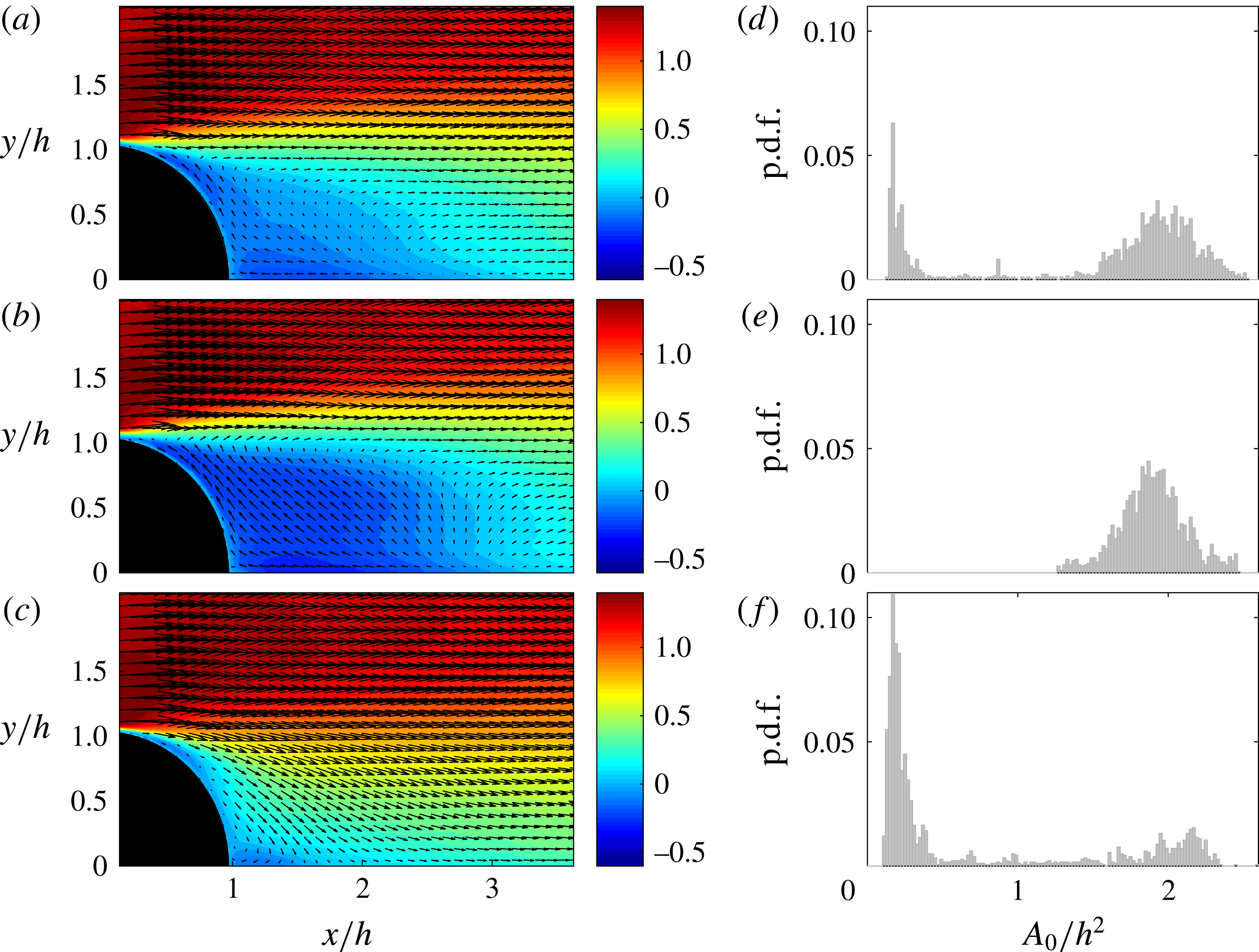
As apparent, for each of the three measurements the mean, i.e. the ensemble average using all 1825 instantaneous velocity fields, was computed and is presented in figure 14(a–c), while the p.d.f. of the low-pass filtered $A_{0}$ in $\unicode[STIX]{x1D6FA}_{3}$ of each of the measurements is presented in figure 14(d–f). Although the three measurements were repeated under the same conditions, the mean flow appears very different from one measurement to another: measurement (b,e) shows a strongly separated flow, while measurement (c,f) depicts a nearly attached flow. The measurement (a,d) on the other hand shows a flow exhibiting a combination of the two previous ones. The study of the p.d.f. of $A_{0}$ of the three measurements confirm the previous observation; measurement (b,e) shows a unimodal p.d.f. centred around $A_{0}/h^{2}=1.9$ , while the p.d.f. of measurement (c,f) contains most data around the value 0.2. The p.d.f. of measurement (a,d) in contrast presents a clear bi-modal behaviour with peak values around 0.2 and 1.9. Separating the two parts of the latest p.d.f. and applying the ensemble averaging method as described in § 5.1 to decompose the flow into modes A and B gives a mode A similar to the measurement in (c,f) and a mode B similar to the one in (b,e). The difference between those three measurements is due to the fact that as the actuation strength, i.e. the driving voltage, increases, the frequency at which the flow experiences alternations between mode A and B decreases and the measurement time is not long enough to always observe both modes, as for instance in measurement (b,e) where only mode B is experienced. This was also observed during the S-PIV measurement of the flow at $x/h=1.98$ with $U_{0}=5~\text{m}~\text{s}^{-1}$ and $V_{d}=12~\text{kV}_{p-p}$ ; only mode B was observed during the measurement time as will be shown in the next section of the paper.

In figure 15(a) a 3-D reconstruction of the two different modes (A and B) are shown for the $10~\text{m}~\text{s}^{-1}$ case with the actuation at $V_{d}=12~\text{kV}_{p-p}$ using only the 2-D PIV measurements data. Seven $yz$ -planes are shown for different streamwise positions and three $xz$ -planes at different wall-normal distances. The left-hand side shows the mode A and the right-hand side the mode B, whereas the upper figures show the streamwise and the lower the wall-normal velocity. The total spanwise width is 1.12 $h$ and the figure is made to show the correct proportions. Further $yz$ and $xz$ planes, complementing the overall picture, are available as supplementary material. Overall figure 15 shows clearly the difference between the two modes, mode A shows a flow that is attached over almost the full width of the domain whereas the opposite is true for mode B. These results confirm the picture obtained from the S-PIV measurements of the $yz$ -planes as shown in figure 12, which shows a rather narrow region of incoming, high streamwise velocity flow towards the wall between two wide, low-velocity regions of flow out from the wall.

Figure 15.

Three-dimensional reconstruction of the modes A and B from 2-D PIV measurements in the $xy$ -plane. Panels (a,c) show the streamwise and the wall-normal components of the velocity, normalised by $U_{0}$ , of mode A respectively, while (b,d) show the streamwise and the normal components of the velocity, normalised by $U_{0}$ , of mode B respectively.

5.3 Proper orthogonal decomposition of stereo measurements

A possible way to extract energetic flow structures in a turbulent environment is to use the so-called proper orthogonal decomposition (POD). This technique was introduced by Bakewell & Lumley (Reference Bakewell and Lumley1967) to detect near-wall flow structures in wall-bounded turbulence and is a methodology to decompose the flow into the most energetic structures in terms of orthogonal modes. For a general description of POD the reader is referred to Berkooz, Holmes & Lumley (Reference Berkooz, Holmes and Lumley1993) and Meyer, Pedersen & Ozcan (Reference Meyer, Pedersen and Ozcan2007).

The snapshot POD method (Sirovich Reference Sirovich1987) is used here since the S-PIV data correspond to 1825 snapshots of the same FOV and the number of snapshots is significantly smaller than the number of spatial measurement points. The data are organised in an $M\times N$ matrix $\unicode[STIX]{x1D650}$ with $M$ corresponding to the number of velocity components used, i.e. here all three, times the number of spatial measurement points or velocity vectors and $N$ is the number of snapshots. The eigenvalues and eigenvectors of the matrix $\unicode[STIX]{x1D650}^{\text{T}}\unicode[STIX]{x1D650}$ , where $\unicode[STIX]{x1D650}^{\text{T}}$ is the transpose, are then computed. The eigenvectors are used to reconstruct the basis of the POD modes, also called spatial modes, ( $\unicode[STIX]{x1D6F7}_{i}$ ) with $0\leqslant i\leqslant N-1$ . The eigenvalues ( $\unicode[STIX]{x1D6EC}_{i}$ ) are proportional to the kinetic energy of the flow field represented by the associated POD mode ( $\unicode[STIX]{x1D6F7}_{i}$ ) (Meyer et al. Reference Meyer, Pedersen and Ozcan2007), by ranking them from the highest to the lowest it is possible to classify the POD modes with the most energetic structures first. The projection of the flow field onto the basis of POD modes gives the POD coefficients, also called time coefficients ( $a_{i}$ ). Finally the flow field can be reconstructed using:

if $K=N-1$ the results should be exactly equal to the ‘input’ flow field, while a value of $K<N$ is used to obtain a low-order reconstruction of the flow field only using the most energetic structures and thereby ‘energy filtering’ the flow. The eigenvalues are also used to compute the relative energy associated with each POD mode as:

Figure 16.

The three first POD modes ( $\unicode[STIX]{x1D6F7}_{0}$ , $\unicode[STIX]{x1D6F7}_{1}$ and $\unicode[STIX]{x1D6F7}_{2}$ ) of the S-PIV measurements at $x/h=1.98$ with $U_{0}=10~\text{m}~\text{s}^{-1}$ for the baseline flow (a) and the actuated flow with $V_{d}=10~\text{kV}_{p-p}$ (b) and $12~\text{kV}_{p-p}$ (c). The velocity components are scaled by an identical arbitrary scale. The colour scale shows the streamwise component of the velocity, i.e. the out-of-plane component, while the arrows show the in-plane motion.

In many applications of the POD technique the mean of the flow is first subtracted, however, here the mean is not removed from the data before applying the POD algorithm. The reason for this is mainly due to the low-frequency nature of the modulation and the associated difficulty in defining a proper mean value for the limited sampling time. This means that the POD analysis is not only on the fluctuating part of the velocity and therefore $\unicode[STIX]{x1D6F7}_{0}$ shows a flow structure similar to the mean flow and contains most of the energy (e.g.  ${>}65\,\%{-}85$  % in the present study). It should be noted that a longer sampling time would be required in case of actuation if the aim were to statistically describe the flow field through the most energetic POD modes (i.e. in terms of a low-order model), as apparent from e.g. figures 9(c) and 14 highlighting the limited number of switches between the two states of the (low-frequency) bi-modality, which is not the case for the baseline case, where the flow is statistically steady (see e.g. figures 5 and 6). The aim of using POD in the present work is hence, to reveal whether there are large-scale streamwise structures inherent in the baseline case, that get amplified through the actuation.

In figure 16, the first three POD modes of the S-PIV in the $yz$ -plane at $x/h=1.98$ of the baseline case and the two actuated cases with $V_{d}=10~\text{kV}_{p-p}$ and $12~\text{kV}_{p-p}$  are shown for the case $U_{0}=10~\text{m}~\text{s}^{-1}$ . The baseline case $\unicode[STIX]{x1D6F7}_{0}$ shows an almost homogeneous distribution of the streamwise velocity in the spanwise direction and the cross-flow velocities do not show any significant structures. 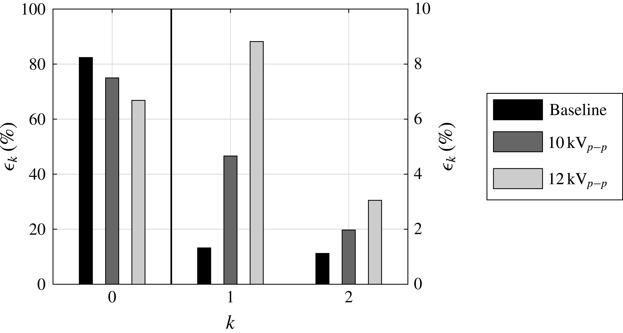The two higher modes $\unicode[STIX]{x1D6F7}_{1}$ and $\unicode[STIX]{x1D6F7}_{2}$ look similar but are almost spanwise mirror images of each other. In figure 17 one can see that more than 80 % of the energy is contained in mode 0 and that modes 1 and 2 have an equal amount of only approximately 1 % each of the total energy. The hypothesis that large-scale streamwise structures are contained also in the baseline flow seems to be a possible explanation for the appearance of two mirror-imaged modes, there is no preferred location of those structures, they are moving randomly in the spanwise direction and are not locked to any specific positions as also seen in figure 9. Therefore there is no preferred phase and modes 1 and 2 have the same energy content and are equally probable.

Figure 17.

Comparison of the energy contained in the three first POD modes of the S-PIV measurements at $x/h=1.98$ with $U_{0}=10~\text{m}~\text{s}^{-1}$ . The black vertical line separates mode 0 to mode 1 and 2 as well as the respective labels.

For the two actuated cases with $V_{d}=10~\text{kV}_{p-p}$ and $12~\text{kV}_{p-p}$  the picture is different. First of all figure 17 shows that the energy in the mean flow is decreasing with increasing $V_{d}$ and correspondingly the energy in $\unicode[STIX]{x1D6F7}_{1}$ and $\unicode[STIX]{x1D6F7}_{2}$ is increasing; for $12~\text{kV}_{p-p}$  the sum of the energy content in these two modes is approximately 12 %. In figure 16 the mean flow mode is less homogeneous for the actuated cases, however, mode 1 for both voltages shows two large-scale structures of different phase. They are, however, almost mirror images of each other, and they also correspond well to modes 1 and 2 for the baseline case. Mode 2 for the two actuated cases are on the other hand very similar. Also for the actuated cases the phase of the signal changes as seen in figure 9, where the structures seem to be locked into two specific positions.

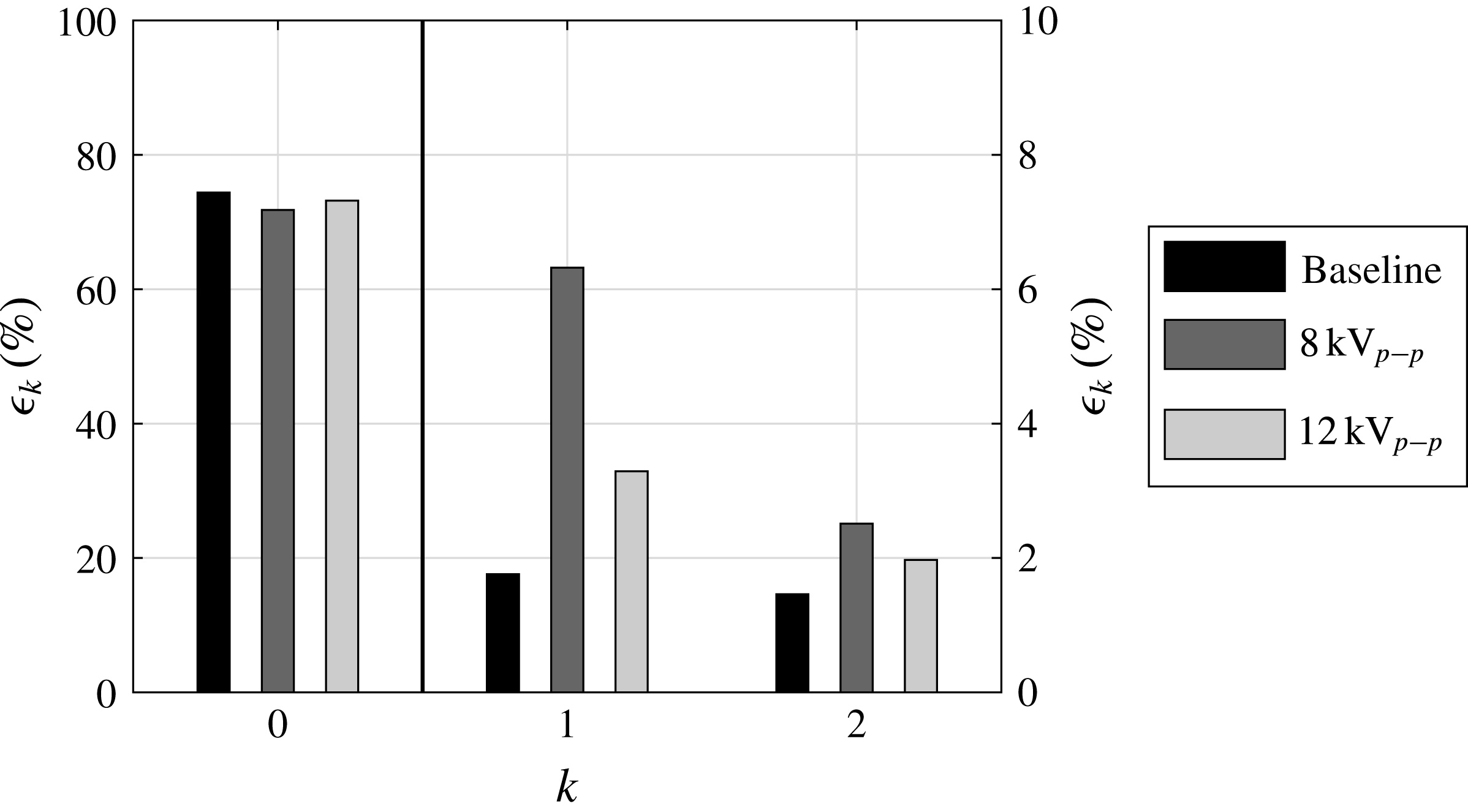
Measurements at $5~\text{m}~\text{s}^{-1}$ are shown in figures 18 and 19, for the baseline case and for $8~\text{kV}_{p-p}$  and $12~\text{kV}_{p-p}$  actuation voltage. When comparing the energy content in the first three modes the picture is quite different as compared to the $10~\text{m}~\text{s}^{-1}$ case, since the relative energy of mode 0 does not change much with the actuation voltage, except that here the $8~\text{kV}_{p-p}$  case shows the smallest relative energy, whereas, mode 1 has the highest relative energy of the three cases. By looking at figure 18 one observes that the baseline case is homogeneous in the spanwise direction which was also observed at $10~\text{m}~\text{s}^{-1}$ , whereas as the actuation voltage increases it becomes more inhomogeneous and at $12~\text{kV}_{p-p}$  a vortical structure can be identified in mode 0, i.e. in the mean flow. This is probably so because the actuation is strong enough to keep the vortex structure locked at one position during most of the time of the measurements. A similar observation can be made from figure 13, where for some of the spanwise positions the flow stays at either mode A or mode B over the full measurement time. Therefore, the vortex structures show up in mode 0 and not in mode 1. On the other hand for $8~\text{kV}_{p-p}$  mode 0 shows a fairly homogeneous spanwise distribution, hence the actuation is probably not strong enough to lock the structures in one place and therefore they show up in mode 1. In this case the baseline and the $8~\text{kV}_{p-p}$  actuation cases show strong similarities although the relative energy content of mode 1 is four times larger for the actuated case.

Figure 18.

The three first POD modes ( $\unicode[STIX]{x1D6F7}_{0}$ , $\unicode[STIX]{x1D6F7}_{1}$ and $\unicode[STIX]{x1D6F7}_{2}$ ) of the S-PIV measurements at $x/h=1.98$ with $U_{0}=5~\text{m}~\text{s}^{-1}$ for the baseline flow (a) and the actuated flow with $V_{d}=8~\text{kV}_{p-p}$ (b) and $12~\text{kV}_{p-p}$  (c). The velocity components are scaled by an identical arbitrary scale. The colour scale shows the streamwise component of the velocity, i.e. the out-of-plane component, the arrows show the in-plane motion.

Figure 19.

Comparison of the energy contained in the three first POD modes of the S-PIV measurements at $x/h=1.98$ with $U_{0}=5~\text{m}~\text{s}^{-1}$ . The black vertical line separates mode 0 from mode 1 and 2 as well as the respective labels.