





1. Introduction
Particle-driven gravity currents arise in many situations in nature and industry, including large turbidity currents that spread from 1 km to hundreds of km over the sea floor (Sparks et al. Reference Sparks, Bonnecaze, Huppert, Lister, Hallworth, Mader and Phillips1993), volcanic ash flows that travel tens of km from volcanic vents (Sparks et al. Reference Sparks, Bursik, Carey, Gilbert, Glaze, Sigurdsson and Woods1997), and particle suspensions produced during deep-sea mining operations (Ouillon et al. Reference Ouillon, Kakoutas, Meiburg and Peacock2021; Peacock & Ouillon Reference Peacock and Ouillon2023). Much research into the dynamics of these flows has focused on the patterns of particle fallout (e.g. Gladstone & Pritchard Reference Gladstone and Pritchard2010) and the impact of the associated change in density on the speed of the current (e.g. Felix & Peakall Reference Felix and Peakall2006).
In some situations, it is important to understand the mixing of the current with ambient fluid: e.g. with an ash flow, the ambient air mixed into the flow may be heated up by the thermal energy in the particles, leading to generation of buoyancy, or in a submarine turbidity current, the ambient fluid may be of different salinity from the source fluid in the current, leading to a change in the ionic concentration of the suspending fluid. This can cause flocculation and hence accelerated sedimentation of any clay particles in the flow. While there have been systematic experimental studies of the process of entrainment in single-phase gravity currents (e.g. Sher & Woods Reference Sher and Woods2015), less is known quantitatively about the entrainment and mixing in particle-driven currents.
Here, we present a series of new experiments to explore the impact of such mixing on particle-driven finite-volume gravity currents. In carrying out our new experiments, we have recognised that the separation of particles from the fluid at the top of the current is also a key process in particle-driven gravity currents. Although such particle–fluid separation is a well-known process in settling columns, it has not been explored in detail in the context of particle-driven gravity currents. The competition between such particle settling, which reduces the current volume, and entrainment, which increases the current volume, forms a central focus of the present work.
To place our work in context, we now review some of the earlier work on single-phase and then particle-driven gravity currents related to our study. Gravity currents are produced from either a finite release or a continuous release of dense fluid into a less dense fluid: in experimental studies of gravity currents, a dense fluid is typically released from one end of a long horizontal flume using either a continuous source or a finite volume of dense fluid, as shown in figure 1. As suggested by this figure, the dynamics of finite-volume gravity currents is different from their continuous-source counterparts: the differences emerge both from the mixing of ambient fluid into the flow and also from the settling of particles from the flow. The sketch in figure 1 has been drawn from some experimental studies that focused on the impact of mixing in these different types of gravity current, as presented by Sher & Woods Reference Sher and Woods2015; Sher & Woods Reference Sher and Woods2017 and Lippert & Woods (Reference Lippert and Woods2020), and the present work. We now review some of these studies, as well as the large body of work modelling the dynamics of gravity currents, to provide context for the present study in which we focus on high Reynolds number currents (
 ${\textit{Re}}_0 \gt 10^4$
) produced by the release of a dense suspension of particles and fluid of finite volume (figure 1
d).
Schematic of the mixing processes for homogeneous and particle-driven gravity currents produced by either a continuous supply or a release of a finite volume of fluid. Models as proposed by (a) Sher & Woods (Reference Sher and Woods2015), (b) Sher & Woods (Reference Sher and Woods2017), (c) Lippert & Woods (Reference Lippert and Woods2020) and (d) the present work.

Figure 1 Long description
A schematic diagram illustrating mixing processes in gravity currents driven by homogeneous and particle-driven fluids under continuous supply and finite-volume release conditions. Panel A: A diagram showing a continuous supply of homogeneous fluid creating a steady gravity current. The wake region of mixed fluid is depicted with arrows indicating entrainment and mixing at the head, and displaced ambient fluid. Panel B: A diagram showing a finite-volume release of homogeneous fluid creating a transient gravity current. The stratified wake is shown with arrows indicating entrainment and mixing at the head, and displaced ambient fluid. Panel C: A diagram showing a continuous supply of particle-driven fluid creating a steady gravity current. The particle-free fluid is depicted with a settling front, and arrows indicating entrainment and mixing at the upper interface, along with sedimentation. Panel D: A diagram showing a finite-volume release of particle-driven fluid creating a transient gravity current. The particle-free fluid is depicted with a settling front, and arrows indicating entrainment and mixing at the head, along with sedimentation.
Prandtl (Reference Prandtl1952) described some of the processes involved in high Reynolds number single-phase gravity currents, including a qualitative picture of the generation of eddies at the head of the flow and the associated mixing with ambient fluid. Subsequently, Huppert & Simpson (Reference Huppert and Simpson1980) presented one of the first detailed experimental studies of single-phase gravity currents produced by a finite release of fluid in the case when the two fluids are miscible. They focused on the speed of the head of the current as a function of time, and found that after an initial slumping phase, as the current becomes established, the speed of the head can be described in terms of a local balance
 \begin{equation} u_h = \textit {Fr}\, (g'h_h)^{1/2}, \end{equation}
where
 $\textit {Fr}$
is the Froude number,
 $g'$
is the reduced gravity of the fluid in the head, and
 $h_h$
is the depth of the head. There have been several different models developed to predict or quantify the value of the Froude number in this relation, and its possible dependence on the ratio of the depth of the head and the fluid,
 $h_h/H$
, using shallow-water theory, or arguments based on Bernoulli-type analyses (Benjamin Reference Benjamin1968; Huppert & Simpson Reference Huppert and Simpson1980; Marino et al. Reference Marino, Thomas and Linden2005; Ungarish Reference Ungarish2023). These models have been tested through experimental studies in which
 $\textit {Fr}$
has been estimated from measurements of the speed and depth of the head of the current (e.g. Marino et al. Reference Marino, Thomas and Linden2005).
There have also been experimental studies exploring the mixing between the ambient and current fluid in finite-volume, single-phase currents (Hallworth et al. Reference Hallworth, Phillips, Huppert and Sparks1993; Sher & Woods Reference Sher and Woods2015). The advent of digital cameras and image processing systems has enabled very detailed measurement of the mixing in these flows. As ambient fluid ahead of the current is displaced up and over the head of the flow, a shear layer develops at the rear of the head; Sher & Woods (Reference Sher and Woods2015) proposed that the entrainment of ambient fluid into the current results in a constant fraction, of order 0.5–0.6 of this displaced fluid, being mixed into the flow, and they tested this picture of the mixing with a series of detailed laboratory experiments.
This mixing of the ambient and current fluid causes the reduced gravity of the fluid to decrease. In a single-phase current produced from a finite volume of fluid, the total buoyancy of the current per unit width,
 $B= g'_0V_0$
, is constant (where
 $V_0$
is the initial volume per unit width), even if the current mixes with ambient fluid, provided that the buoyancy arises from a conserved quantity (e.g. total salt content) and that the change in density is linearly proportional to this quantity. In this case, dimensional analysis suggests that for a unidirectional current, the speed of the current depends on
 $x_h$
, the position of the head, and
 $B$
, the buoyancy per unit width of the current, so that
 \begin{equation} u_h(x_h) = K (B/x_h)^{1/2}, \end{equation}
where
 $K$
is a constant that can be determined empirically from experimental data. According to this scaling law, the position of the head of the current may be re-expressed in terms of time as
 \begin{equation} x_h(t) = \left ( x_h(t_0)^{3/2} +\frac {3K}{2} B^{1/2}(t-t_0) \right )^{2/3}. \end{equation}
Many experimental studies have shown that this model describes the motion of the current for times
 $t\gt t_0$
following the initial slumping phase of the flow (Huppert & Simpson Reference Huppert and Simpson1980; Sher & Woods Reference Sher and Woods2015), and in this phase of the flow, the current approaches a self-similar form. The experiments suggest that
 $\textit {Fr}= 0.7$
, which has been shown to be equivalent to
 $K=1.07$
. Through detailed experimental measurement of the density of the flow, Sher & Woods (Reference Sher and Woods2015) established that in this regime, the current density is stratified both vertically and horizontally: the highest-density fluid advances in the head of the flow, and as ambient fluid mixes into this fluid, the fluid becomes progressively less dense. Data show that the volume can increase by a factor of 4–5 as the current travels through the first 10 lock lengths. In accord with this picture, numerical simulations of particle-driven gravity currents (Necker et al. Reference Necker, Härtel, Kleiser and Meiburg2005) have shown mixing with ambient fluid.
We now turn to the literature on particle-driven gravity currents. The seminal work on such flows was reported by Bonnecaze et al. (Reference Bonnecaze, Huppert and Lister1993), who presented laboratory experiments and a shallow-water model to describe the dynamics. The primary measurements presented in that work were the location of the head of the current as a function of time for a series of currents with different particle fall speeds compared to the buoyancy speed of the initial flow (1.1), but there were also some data on the spatial distribution of the deposit. They presented a shallow-water model in which it was assumed that (i) the particles remained well-mixed throughout the flow and (ii) there was no mixing between the ambient and the current fluid. The model allowed for the sedimentation of particles from the base of the flow, which led to a gradual decrease in the density of the current. At the head of the flow, the current speed was assumed to be governed by a relation of the form (1.1), but now allowing for the density
 $g'$
to decrease gradually owing to the sedimentation. This modelling approach has been developed to account for multiple particle sizes (e.g. Harris et al. Reference Harris, Hogg and Huppert2002) and an integral ‘box model’ has also been proposed (Dade & Huppert Reference Dade and Huppert1995).
These models, which are based on shallow-water theory, predict the speed and run-out distance for the flow based on the rate of sedimentation compared to the rate of advance of the flow. Since the models assume that the flow remains well mixed and that there is no mixing between the ambient and the current fluid (cf. Bonnecaze et al. Reference Bonnecaze, Huppert and Lister1993; Harris et al. Reference Harris, Hogg and Huppert2002), there is an important question about the momentum balance. In particular, for a water-based dilute suspension of particles, the majority of the mass and hence momentum of the current is carried by the host fluid. As the particles sediment from the base of the flow, the current therefore retains the majority of its momentum and mass, but the buoyancy
 $g'$
decreases towards zero. The model for the speed of the head, based on (1.1), then leads to prediction of a deepening and slowing of the head of the current (Bonnecaze et al. Reference Bonnecaze, Huppert and Lister1993). In the present paper, we describe a suite of new experiments, recorded using high-speed video cameras and using light attenuation techniques, to explore the evolution of the current in more detail, and this leads to some new insights about particle-driven gravity currents. As we describe in the paper, our new experiments suggest that as the current approaches the maximum run-out distance, the depth of the head in fact falls to zero. Using dye to visualise the motion of the fluid in the particle-driven current, we also show that particles settle from the fluid at the top surface of the flow. As the flow approaches the maximum run-out distance, this settling of particles leads to a decrease in the volume of the flow, and the momentum of the fluid in the current can then be carried off in the fluid that is released by this settling at the top surface of the flow.
Indeed, literature about settling columns suggests that if the speed of turbulent fluctuations is much larger than the particle fall speed, then the turbulence may act to suspend and mix the particles in the column, but as the turbulence intensity falls, some separation of fluid and particles at the top surface of the suspension may develop (Oliver Reference Oliver1961; Kim & Klima Reference Kim and Klima2004; Akutina et al. Reference Akutina, Revil-Baudard, Chauchat and Eiff2020). This releases particle-free fluid at the top of the suspension. In an analogous fashion, the experiments reported in this paper show that in particle-driven gravity currents, there is some settling of the particles from the top surface of the current, especially in the region behind the head, and this releases particle-free fluid from the top of the current.
Evidence for the importance of such settling at the top of a gravity current has been explored in the context of continuous particle-driven gravity currents by Lippert & Woods (Reference Lippert and Woods2020). In that study, a series of experiments was reported in which a continuous source of particle-driven fresh water was released at the end of a flume filled with fresh water. As the particle suspension travelled along the flume, particles settled through the flow, releasing particle-free fluid across a settling front (figure 1
 $c$
). In addition, some particles sedimented from the base of the flow to the floor of the tank. Eventually, as the fluid continued forwards, the settling front descended to the floor of the tank, and this point marked the leading edge of the particle-laden flow.
The above discussion identifies that there is a competition between the entrainment of ambient fluid into the head of the flow, tending to increase the current volume, and the settling of particles and the release of fluid from the top of the flow, tending to decrease the current volume. Yet, to our knowledge, this aspect of particle-driven gravity currents has not been explored in detail in the literature. Therefore, we have carried out a systematic series of new experiments on particle-driven gravity currents. Our objective is to measure the volume and speed of the current as a function of the position of the head of the flow, to assess the controls on the evolution of the volume as the current evolves along the flume. To help in the interpretation of our new experimental data, it is useful to use a model to provide insight into the controls. To this end, we develop an idealised ‘box model’ for the flow. Although there are box models described in the literature that model the motion of finite-volume single-phase (Huppert & Simpson Reference Huppert and Simpson1980) and particle-driven gravity currents (Dade & Huppert Reference Dade and Huppert1995; Gladstone & Woods Reference Gladstone and Woods2000), these models do not account for the processes of either entrainment of ambient fluid or settling of particles and release of fluid from the top of the flow. Instead, they assume that the volume of the flow is constant. We therefore develop a new box model that combines (i) the entrainment model of Sher & Woods (Reference Sher and Woods2015) for single-phase gravity currents, and (ii) the sedimentation model of Bonnecaze et al. (Reference Bonnecaze, Huppert and Lister1993), but which also includes (iii) a new model for the settling of particles through the top surface of the current. Through use of our new experimental data, we are able to explore and test the model predictions as a function of the ratio
 $S_0$
of the scaling for the current speed
 \begin{equation} u_0 = \textit {Fr}\, (g'_0L_s)^{1/2} \end{equation}
and the particle fall speed
 \begin{equation} v_s = \frac {d_p^2 (\rho _p - \rho _a)g}{18\eta _a} \end{equation}
as defined by
 \begin{equation} S_0 = \frac {u_0}{v_s}, \end{equation}
where the initial buoyancy is
 $g'_0$
, and
 $L_s = (L_0H_0)^{({1}/{2})}$
, where the depth and length of the lock gate are
 $H_0$
and
 $L_0$
,
 $\eta _a$
is the viscosity of water, and
 $d_p$
is the particle diameter.
The ranges of values of
 $S_0$
and of the Reynolds number explored in our experiments overlap with many previous studies, as shown in table 1; the novelty in the present paper is the analysis of these new experiments to measure the evolution of the volume of the current with position of the head of the current, and to interpret this in terms of the different processes. For convenience, throughout this paper, ‘volume’ refers to ‘volume per unit width’ of the gravity current.
Comparison of previous experimental and modelling studies of particle-laden gravity currents produced from a finite volume of fluid. Entrainment: incorporation of ambient fluid. Settling: particle settling from the top surface of the flow. Sedimentation: explicit representation of the basal deposition of particles in the governing equations. Here,
 $S_0$
is the ratio of the initial velocity scale of the current to the settling velocity, and
 ${\textit{Re}}_0$
is the initial Reynolds number.

Table 1 Long description
A table comparing studies of particle-laden gravity currents. The table has six rows and seven columns. The columns are labeled Paper, Type of gravity current, Entrainment, Settling, Sedimentation, S0, and Re0. The rows list different studies with their respective data. Row 1: Bonnecaze et al. (1993), Finite-volume particle-driven, X, X, Checkmark, 70-200, 15000-45000. Row 2: Sher & Woods (2017), Finite-volume particle-driven, X, Checkmark, Checkmark, 6-23, 40000-72000. Row 3: Lippert & Woods (2020), Steady particle-driven, Checkmark, Checkmark, Checkmark, 5-170, 500-1600. Row 4: Tonoyama & Woods, Finite-volume particle-driven, Checkmark, Checkmark, Checkmark, 5-1100, 12000-40000.
We have arranged the paper as follows. First, we describe our experiments, and present new measurements of the evolution of the volume of particle-driven gravity currents to explore the competition between (i) entrainment, as the head of the current displaces ambient fluid up and over the current, (ii) settling of particles from the surface of the flow, and (iii) sedimentation of particles from the base of a particle-driven current. This leads to a new picture of the evolution of the volume of the current with distance from the source, and of the rate of mixing of ambient fluid into the current. We then compare the experimental data with a ‘box model’, which provides a simplified quantification of the entrainment, the settling and the sedimentation.
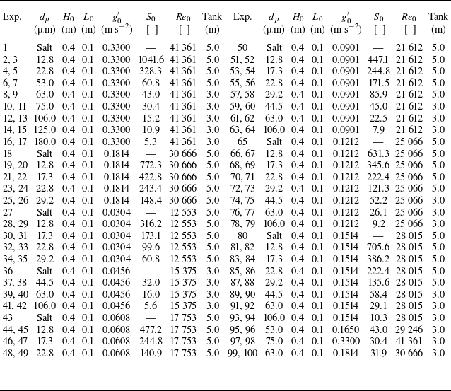
Table of experimental parameters; a smaller experiment number indicates that no dye was used, whereas a larger number indicates that dye was added to the fluid behind the lock gate. Here, we give particle diameter (
 $d_p$
), height and length of the fluid behind the lock gate (
 $H_0, L_0$
), the ratio of the current velocity scale to the settling velocity (
 $S_0$
), and the Reynolds number (
 ${\textit{Re}}_0$
).

Table 2 Long description
A table with 50 rows and 14 columns comparing experimental parameters for fluid dynamics studies. The columns are labeled as follows: Exp., d_p (µm), H_0 (m), L_0 (m), g’_0 (m s^-2), S_0, Re_0, Tank (m), Exp., d_p (µm), H_0 (m), L_0 (m), g’_0 (m s^-2), S_0, Re_0, Tank (m). The table presents data for experiments with and without dye, showing particle diameter, height and length of the fluid behind the lock gate, the ratio of the current velocity scale to the settling velocity, and the Reynolds number. The experiments are grouped into pairs, with each pair sharing similar parameters but differing in the use of dye.
2. Experimental method
We have carried out a series of experiments in two different flumes, each of width 0.1 m, depth 0.5 m, which are 3 and 5 m long. Silicon carbide particles (
 $\rho _p = 3217$
kg m−3, Washington Mills) were mixed with fresh water (
 $\rho _a = 998$
kg m−3) and then released from behind a lock gate located 0.1 m from one end of the tank. The fluid in the tank was 0.4 m deep. A series of experiments was run with different particle loads (
 $g^{\prime }_0 = 0.0304{-}0.33$
m s−2) and sizes (
 $d_p = 12.8{-}180$
 ${\unicode[Arial]{x03BC}}$
m) as listed in table 2, and a single-phase aqueous saline current of the same initial buoyancy was run as a reference in each case. The experiments were repeated with the fluid behind the lock gate being dyed red or being clear so that the fate of the particles and the original suspension fluid could be followed. For the dyed experiments, 0.75 g l−1 of TRS red food dye was mixed inside the lock gate, and to compensate for the change in density of this fluid, 0.6 g l−1 of salt was stirred into the ambient water so the solutions had the same density. The densities of the different aqueous solutions were measured by weighing a fixed volume of each solution; these were also compared with density tables from the CRC Handbook of Chemistry and Physics. The experiments were recorded by video using Nikon D5300 cameras, with the tank being back-lit by an electroluminescent light sheet (W & Co Displays and Signs).
Photographs of (
 $a$
) a saline gravity current, Exp. 1; (
 $b$
) a particle-driven gravity current with no dye in the source fluid, Exp. 8; (
 $c$
) a particle-driven gravity current with the source fluid dyed, Exp. 9. In each image, the green line, obtained by thresholding the light intensity of the image, indicates the top of the current as a function of distance along the tank.

Images were analysed using MATLAB in order to identify the volume of the current, and as far as was possible, to measure the particle load, as a function of position in the current. There are two different volumes that we measure: first, the volume of the particle-driven flow, and second, the volume of fluid into which the fluid behind the lock gate has mixed. In order to measure the volume of the particle-driven current, we do not use any dye. We take a reference image prior to the start of the experiment. Once the current is released from the lock and runs along the flume, we subtract the reference image from each of the series of images of the evolving current. We then assess the location of the edge of the current by using a small threshold value for the change in light intensity of each pixel. By varying the value of this threshold, we estimate that our measurement of the current volume is accurate to within 5
 $\,\%$
for a given experiment. In order to measure the volume of fluid into which the fluid behind the lock gate has mixed, we carry out a second experiment in which we add dye to the particle-driven fluid behind the lock gate. We then use the same thresholding technique to detect the edge of the region of dyed fluid.
Figure 2 illustrates the result of the edge-detection algorithm for a photograph taken from each of three experiments. First, we show a single-phase saline current; second, we show a particle-driven current with no dye; and third, we show a particle-driven current with dye. In each case, the top boundary of the current is shown by the green line.
To measure the particle load in the current, calibration experiments were carried out in which the tank was filled with a series of suspensions of different known particle loads, and in each case, a series of photographs were taken. The particle-driven fluid becomes opaque above a certain particle concentration, so it is hard to measure the full distribution of particle load using light attenuation. However, as the concentration falls below approximately 10
 $\,\%$
of the initial value in our experiments, it is possible to measure variations in the light intensity. This enables us to relate the light intensity, averaged across the width of the tank, to the width-averaged particle load, in cases in which the fluid had no dye. To measure the particle load in an experiment, we take a series of images of a current as it moves along a tank, and using the calibration curve, we convert the light intensity to particle load, averaged across the width of the tank, as the current evolves along the tank.
The turbulent fluctuations in the flow can lead to some variability in the measured volume between different experiments using the same source conditions. We have therefore repeated several of the experiments, and find that the instantaneous volume varies by up to
 $10 \,\%$
between otherwise identical experiments. An example of this is shown in Appendix.
In order to parametrise the experiments (table 1), the initial reduced gravity is given by
 \begin{equation} g^{\prime }_0 = \phi _0 g(\rho _p-\rho _a)/\rho _a, \end{equation}
where the initial volume fraction of particles is
 $\phi _0$
, the particle and fluid densities are
 $\rho _p$
and
 $\rho _a$
, and
 $g$
is the gravitational acceleration. In each experiment, the volume fraction of particles
 $\phi _0$
was calculated by combining the density of the particles and the density of the solution, with the measurement of the mass of particles
 $m_p$
that were mixed with a mass
 $m_a$
of aqueous solution, so that
 \begin{equation} \phi _0 = \frac {m_p/\rho _p}{(m_p/\rho _p) + (m_a/\rho _a)}. \end{equation}
The speed of the head
 $u_h$
is scaled with
 $u_0$
in (1.4). The particle settling velocity
 $v_s$
for the present particles, of diameter
 $d_p$
, was based on data presented by Lippert & Woods (Reference Lippert and Woods2020) using the Stokes settling speed
 $v_s$
in (1.5) The currents are characterised in terms of the parameter
 $S_0$
in (1.6), which compares the scaling for the current speed in (1.4) with the particle fall speed.
The Reynolds number of the currents is defined as
 ${\textit{Re}}_0=(u_0 L_s)/\nu _w$
, where,
 ${\nu _w} = 1.0\times 10^{-6}$
m
 $^2$
s−1 is the kinematic viscosity of water. In all the experiments, this exceeds
 $\sim 10\,000$
, so the flows rapidly become fully turbulent following release from the lock gate.
3. Experimental observations
In figure 3, we illustrate three series of photographs of gravity currents with the same initial buoyancy. For reference, figure 3(
 $a$
) shows a series of images of a single-phase current of an aqueous salt solution, and figure 3(
 $b$
) corresponds to a particle-driven gravity current. The frames are taken at time intervals of 1.8 s. As these currents advance along the base of the tank, the volume initially increases as ambient fluid ahead of the current is displaced upwards over the head of the flow, and some of this fluid mixes into the current (cf. Sher & Woods Reference Sher and Woods2015). This leads to formation of a tail of mixed fluid, and dilution of the head. In the particle-driven flow (figure 3
 $b$
) some of the particles settle out from the tail, eventually leading to a reduction in the volume of particle-driven fluid.
Series of photographs showing the time evolution of: (
 $a$
) a saline gravity current, at intervals of 1.8 s, Exp. 1; (
 $b$
) a particle-driven gravity current with clear source fluid, at intervals of 1.8 s, Exp. 8; (
 $c$
) a particle-driven gravity current with the source fluid dyed red, at intervals of 1.8 s, Exp. 9. Experiments (
 $a$
–
 $c$
) had initial buoyancy
 $g^{\prime }_0=0.33$
, and the particle diameter (b,c) is 63
 ${\unicode[Arial]{x03BC}}$
m, so (b,c)
 $S_0$
= 43.0.

A complementary understanding of the evolution of the source fluid in the particle-driven gravity current can be seen in the third set of images, in which the source fluid is dyed red (figure 3
 $c$
). On release from the lock gate, the source fluid spreads out in the tail as well as the head of the flow. As particles settle through the tail, the fluid develops a vertical particle stratification, with the upper part of the tail being nearly particle-free and red, while the lower parts are much darker owing to the presence of particles. The volume of the particle-bearing region of the current initially increases but then decreases as the particles settle from the flow. However, the volume of red-dyed fluid continues to increase. Once the particles settle from the tail, eddies in the particle-free dyed fluid appear to engulf and mix more ambient fluid. This may be contrasted with the saline current in figure 3(
 $a$
), in which the depth of the fluid in the tail remains much smaller.
We define the depth of the head using a light attenuation technique in the region just behind the front of the current,
 $x_h-L_0\lt x\lt x_h$
. In particular, in this region, we find the maximum depth above the base of the tank at which the light attenuation, relative to the background (no current) value, exceeds a threshold. The threshold has been varied to ensure that our measurements are consistent within an error of
 $5\,\%$
. In virtually all the experiments, the depth of the head appears to remain close to
 $(0.4\pm 0.05) H_0$
, where
 $H_0$
is the depth of the water in the flume. This observation is consistent with previous observations of single-phase aqueous gravity currents (cf. Sher & Woods Reference Sher and Woods2015).
Indeed, in figure 4(a), we present a graph of the evolution of the volume of the current, and in figure 4(b), the depth of the head of a typical current as a function of the distance downstream. As expected, it is seen that the volume increases owing to the entrainment and mixing, while the depth of the head of the current remains close to
 $0.4H_0$
. Eventually, the volume reaches a maximum then decreases to zero, but the data suggest that regardless of whether the volume increases or decreases, the depth of the head remains approximately constant until just before reaching the maximum run-out distance. In the next section, we explore this in more detail for a series of currents with different values of
 $S_0$
.
Variation of (
 $a$
) the volume and (
 $b$
) the height of the current head as a function of time. Regardless of whether the volume increases or decreases, the current continues to propagate while maintaining an approximately constant head height until just before the run-out distance of the current. (
 $c$
) Series of false colour images from Exp. 99, with
 $d_p = 63.0$
 ${\unicode[Arial]{x03BC}}$
m,
 $S_0 = 31.9$
, which show the evolution of the regions of different particle concentration as a function of distance downstream
 $x/L_s$
. Particle concentration is shown in the legend. (
 $d$
) Variation of the volume of particle-laden fluid with concentration in excess of different fractions of the initial particle concentration as a function of the position of the head of the current. The colour categories correspond to different concentrations shown in the legend, and the volumes are scaled by
 $L_s^2$
.

Figure 4 Long description
Panel A: A line graph shows the variation of the volume of the current head as a function of time. The x-axis is labeled ‘t/√(L_s/g_0’)‘ and the y-axis is labeled ‘V/L_s^2’. The data points form a curve that rises to a peak and then gradually declines. Panel B: Another line graph displays the height of the current head as a function of time. The x-axis is labeled ‘t/√(L_s/g_0’)’ and the y-axis is labeled ‘h_h/H_0’. The data points fluctuate around a relatively constant value with a slight downward trend. Panel C: A series of false color images show the evolution of regions with different particle concentrations as a function of distance downstream. The x-axis is labeled ‘x_h/L_s’ and the color legend indicates different concentration ranges from less than 2 percent to over 10 percent. Panel D: A scatter plot illustrates the variation of the volume of particle-laden fluid with concentration in excess of different fractions of the initial particle concentration as a function of the position of the head of the current. The x-axis is labeled ‘x_h/L_s’ and the y-axis is labeled ‘V/L_s^2’. Different colored data points represent different concentration ranges as indicated in the legend.
To illustrate the interior structure of the current, we have used the light attenuation technique to assess the evolution of the particle load in the current in more detail. In figure 4(
 $c$
), we present a series of images in which we show the spatial distribution of the particle load as the current advances along the flume. The different colours in each image denote different concentration values as a fraction of the initial concentration, as shown in the colour bar. The figure illustrates that a significant vertical and lateral stratification of particle concentration develops in the current, with the fluid in the head being of the highest concentration. Using the particle concentration data in the current, we have calculated the volume of fluid in the current in which the concentration exceeds a series of different values as a function of the position of the head of the current. This is shown in figure 4(
 $d$
). As the current advances along the flume, the volume exceeding each particle concentration initially increases but eventually reaches a maximum, and then decreases to zero.
The time and hence position of the head at which the maximum volume is reached increases as the concentration falls, eventually leading to a plot similar to figure 4(
 $a$
) of the total volume.
The data also show that the volumes of fluid with concentrations in excess of
 $6\,\%$
and
 $10\,\%$
of the initial concentration evolve in a very similar way. This corresponds to the region of relatively high particle load, which is located mainly in the head. As the particles settle through the current, and more ambient fluid is mixed into the current, a region of progressively smaller concentration forms, especially in the upper part of the flow (see the first five rows of figure 4
 $c$
). In part, this results from the separation of the fluid and particles at the top of the particle-driven flow, as a result of particle settling.
Figure 4(
 $c$
) also illustrates that the tail of the current is composed of a series of eddy-type structures, with relatively low particle concentration. These structures do not advance very far along the flume before the particles settle to the base of the flume, releasing particle-free fluid into the ambient. Meanwhile, the head continues advancing down the flume. The key processes observed in the experiments are sketched in figure 1(
 $d$
), illustrating the mixing, settling and sedimentation.
Experimental measurement of: (
 $a$
) the volume of a particle-driven gravity current as a function of distance of the head from the source; (
 $b$
) the distance of the head from the source as a function of time; and (
 $c$
) the height of the head as a function of the position of the head, scaled by the position of the head when the volume is a maximum. In (
 $a$
), the open symbols correspond to the particle-driven fluid in experiments using undyed source fluid, while the solid symbols correspond to the volume of dyed fluid in an equivalent experiment in which the source fluid was dyed (
 $d_p = 12.8{-}180$
 ${\unicode[Arial]{x03BC}}$
m,
 $g^{\prime }_0=0.33$
m s−2, Exp. 1–17). The dashed line in (
 $a$
) corresponds to the rate of increase of volume of a single-phase gravity current (Sher & Woods Reference Sher and Woods2015). In (
 $c$
), curves are shown for a range of values of
 $S_0$
as indicated in the legend in (a).

4. Quantitative measurements
In order to understand the relative rates of the different processes controlling the evolution of the flow, we now explore the impact of variations in
 $S_0$
on the evolution of the volume, the speed, and the height of the head of the current.
In figure 5(
 $a$
), we present a series of experimental measurements of the volume of the particle-driven fluid (open symbols) and of the fluid containing dye that originates behind the lock gate (solid symbols). Both are shown as a function of the distance of the head of the current from the rear of the lock gate. The volume is normalised by the initial volume behind the lock gate,
 $L_s^2$
, and the position of the head,
 $x_h$
, is normalised by the length scale of the flow,
 $L_s$
. The different experiments correspond to different particle sizes, as shown in the legend for the plot, and for a fixed total initial current buoyancy. The currents all have different values of
 $S_0$
. The dashed line corresponds to the rate of change of the volume of a saline gravity current, as measured by Sher & Woods (Reference Sher and Woods2015).
During the initial phases of the flow, the volumes of both the dyed fluid and the particle-driven fluid increase at a similar rate to the reference saline gravity current. However, eventually, the volume of the particle-driven fluid reaches a maximum, and as the flow continues downstream, this volume begins to fall. We interpret this as the point at which settling of particles from the top surface of the flow exceeds the rate of mixing of ambient fluid into the head, and a layer of particle-free dyed fluid develops above the current (cf. figure 2
 $c$
). This fluid retains its forward momentum, but loses the buoyancy associated with the particle load. It is then able to mix more readily with the overlying ambient fluid, so the volume of fluid that contains red dye continues to increase with time. The data for the single-phase saline current shown by the black crosses show the same increase in volume with distance for
 $x_h/L_s \lt 10$
, but as the flow travels further from the lock gate, there is a gradual decrease in the rate of increase of volume; this may be the result of bottom friction (cf. Sher & Woods Reference Sher and Woods2015).
In figure 5(
 $b$
), we illustrate the position of the head of the current as a function of time, scaled with the characteristic time for the gravity current
 $\sqrt {L_s/g'_0}$
for currents with a range of values of
 $S_0$
. This figure illustrates that the currents all initially have a comparable speed, but for smaller values of
 $S_0$
, the particles settle through the fluid progressively more quickly, and the flow does not travel as far along the flume before slowing down and waning. As a result, the maximum volume and the overall run-out length of the current decrease.
In figure 5(
 $c$
), we show the scaled height of the head of the current as a function of position of the head scaled by
 $x_{V_{\textit{max}}}$
, the position of the head at which the maximum volume is reached. Curves are shown for a large range of values of
 $S_0$
. This figure illustrates that for all currents, the depth of the current remains close to
 $(0.4\pm 0.05)H$
as the current advances to points beyond approximately
 $x_h = 1.2x_{V_{\textit{max}}}$
, but then it begins to decrease to zero as the current wanes and all the particles sediment to the base.
We have measured the maximum volume of the particle-driven current, and the dimensionless position of the head at which the current reaches this volume; the data are shown in figure 6. As
 $S_0$
increases, the current travels further before reaching the maximum volume (figure 6
a). Also, there appears to be a strong, and nearly linear, relationship between the maximum volume and the distance at which this is attained for a range of values of
 $S_0$
,
 $30 \lt S_0\lt 300$
(figure 6
b). With larger values of
 $S_0$
, the current reaches the distal end of the flume prior to reaching the maximum volume. As
 $S_0$
increases, the settling slows down, and the current is able to entrain more fluid prior to reaching the maximum volume. Figure 6(c) shows the position of the distal end of the current as a function of
 $S_0$
, illustrating that the maximum run-out distance increases with
 $S_0$
.
Experimental measurement of (
 $a$
) the position of the head when the current reaches the maximum volume as a function of
 $S_0$
, and (
 $b$
) the maximum volume as a function of the position of the head when the current reaches the maximum volume. Points are shown for a range of values of
 $S_0$
in (a). (
 $c$
) The position of the head at the distal end of the current as a function of
 $S_0$
. The curves are predictions from the box model, and error bars denote a 10 % error in distances.

Figure 6 Long description
Three scatter plots compare experimental data with model predictions for particle-driven gravity currents. Panel A: A scatter plot shows the position of the head when the current reaches the maximum volume as a function of S0. The x-axis is labeled S0, and the y-axis is labeled xVmax. The plot includes experimental data points and a model prediction line. Panel B: A scatter plot shows the maximum volume as a function of the position of the head when the current reaches the maximum volume. The x-axis is labeled xVmax, and the y-axis is labeled Vmax. The plot includes experimental data points and a model prediction line. Panel C: A scatter plot shows the position of the head at the distal end of the current as a function of S0. The x-axis is labeled S0, and the y-axis is labeled xterm. The plot includes experimental data points and a model prediction line. Error bars denote a 10 percent error in distances.
5. Box model development
In order to illustrate the competing effects of entrainment and settling on the current volume, as a function of
 $S_0$
, it is helpful to use a ‘box model’ approach to describe the evolution of the current (cf. Huppert & Simpson Reference Huppert and Simpson1980; Sher & Woods Reference Sher and Woods2015). Although such box models are simplified and do not describe all details of the flow, they do have value in providing insight. In this section, we motivate a new box model from the physical processes that we have described, which influence the boundary conditions, coupled with the underpinning equations for fluid and particle conservation. Figure 7 provides a reference for the properties of the current defined in the model.
Schematic of the particle-driven current to illustrate the definitions of the variables used in the box model.

If we consider a small element of fluid in the current lying between
 $x$
and
 $x+\delta x$
, and spanning the depth of the current,
 $0\lt y\lt h(x,t)$
, then the rate of change of the volume of this element of the current in some interval of time,
 ${\partial h(x,t)}/{\partial t}$
, can be expressed as
 \begin{equation} \frac {\partial h}{\partial t} =- \frac {\partial (h\overline {u})}{\partial x} - v_s, \end{equation}
where the first term on the right-hand side denotes the difference between the horizontal flux into and out of the volume, with
 \begin{equation} h\overline {u} = \int _0^h u\, \text{d}y, \end{equation}
and the second term on the right-hand side represents the loss of fluid associated with any settling of the particles at the top surface of the flow, assumed to occur with speed
 $v_s$
. We note that since the flow is turbulent, there may be some resuspension of particles in the flow that suppresses the particle settling (cf. Blanchette & Bush Reference Blanchette and Bush2005; Guazzelli & Hinch Reference Guazzelli and Hinch2011; Lippert & Woods Reference Lippert and Woods2020). This effect is likely to depend on the local ratio of the current speed compared to the particle fall speed. Near the head of the current where the turbulence is very intense, many of the particles may remain suspended, but in the growing tail of the current, behind the advancing head, the flow is less intense, and the capacity for the current to resuspend particles gradually decreases. We therefore assume, for simplicity, that the particles settle with their fall speed
 $v_s$
along the top surface of the current, noting that this approximation should become progressively more accurate as the lateral extent of the current becomes larger than the length scale of the head of the current.
In general, the volume of the current can be written in the form
 \begin{equation} V = \int _0^{x_h(t)} h(x,y)\, \text{d}x, \end{equation}
where
 $x_h$
is the location of the nose of the flow. Using the integral expression for
 $V$
in (5.3), we find that
 \begin{equation} \frac {\text{d}V}{\text{d}t} = h_h \frac {\text{d}x_h}{\text{d}t}- \int _0^{x_h(t)} \frac {\partial h}{\partial t}\, \text{d}x . \end{equation}
Substituting (5.1) then leads to the relation
 \begin{equation} \frac {\text{d}V}{\text{d}t} = h_h \frac {\text{d}x_h}{\text{d}t}- h_h \overline {u_h}- v_s x_n. \end{equation}
Following Sher & Woods (Reference Sher and Woods2015), we note that the entrainment of fluid in the head of the flow leads to the relation (their (4.17))
 \begin{equation} \overline {u_h} = (1-\alpha ) \frac {\text{d}x_h}{\text{d}t}, \end{equation}
so that in the present case,
 \begin{equation} \frac {\text{d}V}{\text{d}t} = \alpha h_h \frac {\text{d}x_h}{\text{d}t} - v_s x_h . \end{equation}
This equation reduces to the result of Sher & Woods (Reference Sher and Woods2015) in the limit
 $v_s=0$
, corresponding to a single-phase saline aqueous gravity current.
We now consider the local conservation of particles:
 \begin{equation} \frac {\partial g'}{\partial t} + \boldsymbol{u}\boldsymbol{\cdot }\boldsymbol{\nabla }g' = -v_s\frac {\partial g'}{\partial y} . \end{equation}
If we integrate over the depth of the flow, then we obtain the relation
 \begin{equation} \frac {\partial }{\partial t} (\hat {g'}(x,t)\,h) + \lambda \frac {\partial }{\partial x} (\overline {u} \hat {g'}(x,t)\,h) = -\beta \hat {g'}(x,t)\, v_s, \end{equation}
where
 \begin{equation} \hat {g'}h = \int _0^h g'\,\text{d}y,\quad \lambda \overline {u} \hat {g'}h = \int _0^h u g'\,\text{d}y,\quad \beta \hat {g'} = g'(0,x,t) . \end{equation}
Here,
 $\lambda$
is a constant associated with any vertical variations in the horizontal velocity and/or the particle load, while
 $\beta$
relates the concentration at the base of the flow to the mean concentration. Equation (5.9) is equivalent to that presented by Bonnecaze et al. (Reference Bonnecaze, Huppert and Lister1993), but in that earlier work, it was assumed that
 $\lambda = 1$
and
 $ \beta = 1$
, corresponding to a well-mixed flow. We also adopt this simplification in the present idealised box model, and test the model with our experimental data that span the range
 $30 \lt S_0 \lt 300$
.
The total particle load in the current is given by
 \begin{equation} \overline {g'}V = \int _0^{x_h} \hat {g'}(x,t)\,h\,\text{d}x , \end{equation}
so differentiating with time, we find
 \begin{equation} \frac {\text{d}(\overline {g'}V)}{\text{d}t} =\frac {\text{d}x_h}{\text{d}t} \left [ \int _0^{h(x_h)} g'|_{x_h}\,\text{d}y \right ] + \int _0^{x_h} \frac {\partial (\hat {g'}h)}{\partial t}\,\text{d}x . \end{equation}
If we substitute the expression for
 ${\partial (\hat {g'}h)}/{\partial t}$
in the last term on the right-hand side, as given by (5.9), we find that this equation becomes
 \begin{equation} \frac {\text{d} (\overline {g'} V) }{\text{d}t} = \frac {\text{d}x_h}{\text{d}t} \left [ \int _0^{h(x_h)} g'|_{x_h}\,\text{d}y \right ] - \left [ \int _0^{h(x_h)} u g'|_{x_h}\, \text{d}y \right ]- \overline {g'} x_h v_s, \end{equation}
where for the last term, for simplicity, we assume that the particle load is uniform along the length of the flow, so that
 $\int _0^{x_h} \hat {g'}\, \text{d}x = \overline {g'} x_h$
. The first two terms on the right-hand side are associated with the entrainment of ambient fluid at the nose of the flow; this does not change the particle load of the current, so these terms add to zero (cf. Sher & Woods Reference Sher and Woods2015). This leads to the relation
 \begin{equation} \frac {\text{d}(\overline {g'} V)}{\text{d}t} = - \overline {g'} x_h v_s. \end{equation}
This equation is equivalent to that in the box models of Bonnecaze et al. (Reference Bonnecaze, Huppert and Lister1993) and Dade & Huppert (Reference Dade and Huppert1995).
To complete the model, we draw on the existing literature and use (1.1) to specify the speed of the head of the flow:
 \begin{equation} \frac {\text{d}x_h}{\text{d}t} = \textit {Fr}\, (\overline {g'}h_h)^{1/2} . \end{equation}
For convenience, we scale the system so that the dimensionless volume, distance, buoyancy, depth of the head, and time (denoted by subscript
 $s$
) are given by
 $ V_s = V/L_s^2$
,
 $ x_s = x_h/L_s$
,
 ${g^{\prime }_s}=\overline {g^{\prime }}/g^{\prime }_0$
,
 $h_s=h_h/L_s$
and
 $ t_s = t/(L_s / g^{\prime }_0)^{1/2}$
.
Combining the equation for the speed of the head (5.15) with that for the rate of change of the volume with time (5.7) leads to the dimensionless equation for the rate of change of volume as a function of the position of the head,
 \begin{equation} \frac {\text{d}{V_s}}{\text{d}{x_s}} = \alpha h_s - \frac { x_s }{ S_0 {g'_s}^{1/2}h_s^{1/2} }, \end{equation}
and the rate of change of the product of the buoyancy and volume with position of the head,
 \begin{equation} \frac {\text{d}(g'_sV_s)}{\text{d}{x_s}} = - \frac { x_s {g'_s}^{1/2} } { S_0 {h_s}^{1/2} }, \end{equation}
while the position of the head increases with time according to the relation
 \begin{equation} \frac {\text{d}x_s}{\text{d}t_s} = \textit {Fr}\, {g'_s}^{1/2} h_s^{1/2}. \end{equation}
The three equations (5.16)–(5.18) determine the evolution of the current volume
 $V_s$
, nose position
 $x_s$
, and particle load
 $g'_s$
, as a function of time. The main parameter controlling the evolution of the current is
 $S_0$
, which appears in (5.16). The initial conditions for our experiments are
 $x_s=L_0/L_s=0.5$
,
 $V_s=1$
and
 $g'_s =1$
. Motivated by the data in figure 5(
 $c$
), we assume that the depth of the head is constant and given by
 $h_h=0.4H_0$
. We now compare the solutions of (5.16)–(5.18) with our data.
First, we note that the equation for the evolution of the volume includes the term proportional to
 $\alpha$
that parametrises the entrainment through the head of the flow. Near the source, the current volume increases nearly linearly with the position of the head (figure 5
 $a$
). The best-fit value for the rate of increase of this volume with position of the head,
 $\alpha h_s$
, in the region
 $0\lt x_s\lt 0.5 x_{V_{\textit{max}}}$
, suggests that
 $\alpha \sim 0.6 \pm 0.1$
. This is consistent with the value of
 $\alpha$
found for a saline current (cf. Sher & Woods Reference Sher and Woods2015), as also shown in the figure. The second term in (5.16), corresponding to the settling of particles through the top surface of the current, is new, and becomes progressively more important as the flow travels further along the flume. As a result, the volume of particle-driven fluid reaches a maximum and then begins to decrease. We have measured the maximum volume of the current
 $V_{\textit{max}}$
, and the position of the head at this maximum volume
 $x_s(V_{\textit{max}})$
, for a number of experimental currents, covering a large range of values of
 $ S_0$
,
 $30 \lt S_0 \lt 300$
. The model predictions for the maximum volume and the head position at the maximum volume as a function of
 $ S_0$
are compared with the experimental data in figures 6(a) and 6(b). The model captures the trend in the experimental data.
Our experiments show that once the current has reached the maximum volume, the height of the head remains at value
 $0.4H_0$
for some distance, but then begins to decrease, and falls to zero at the end of the flow, when all the particles have separated from the fluid; as a result, we do not expect the model to be fully accurate in this region. However, we have compared the prediction of the model for the final run-out distance with the experimental data for those experiments that did not reach the end of the experimental flume. This comparison is shown in figure 6(
 $c$
) as a function of
 $S_0$
. The trend of increasing run-out distance with
 $ S_0$
in the data is also seen in the model, but we note that there is some scatter in the experimental data.
Experimental observations from a range of particle-laden gravity currents (
 $d_p = 12.8{-}106.0$
 ${\unicode[Arial]{x03BC}}$
m,
 $g'_0 = 0.030{-}0.33$
m s−2,
 $S_0 = 10.3{-}1041.6$
, Exp. 2, 34, 55, 76, 93) illustrating (
 $a$
) the volume as a function of distance, and (
 $b$
) the nose position as a function of time. The symbols correspond to measurements from the experiments, and the solid lines correspond to the idealised box model.

Figure 8 Long description
Two line graphs illustrate experimental observations of particle-laden gravity currents. Panel A shows the volume as a function of distance, while Panel B shows the nose position as a function of time. In Panel A, the x-axis represents the normalized horizontal distance (xh/Ls) and the y-axis represents the normalized volume (V/Ls^2). Different colored lines and circles represent various initial conditions (S0 values). The solid lines correspond to the idealized box model, while the circles represent measurements from the experiments. Panel B shows the x-axis as normalized time (t/√(Ls/g’0)) and the y-axis as normalized nose position (xh/Ls). Similar to Panel A, different colored lines and circles represent various initial conditions, with solid lines for the model and circles for experimental measurements. The graphs show how the volume and nose position evolve over time and distance, highlighting the competition between entrainment of ambient fluid and particle settling.
In the experiments, for values of
 $S_0$
smaller than approximately 30, the particles tend to settle from the flow more rapidly, within a distance of a few lock lengths from the source, and this coincides with the initial slumping phase of the flow (cf. Huppert & Simpson Reference Huppert and Simpson1980); for this range of values, the model is less applicable.
In figure 8, we compare the predictions of the idealised box model with data from five example experiments, with different values of
 $S_0$
, in which we have measured the volume of the flow as a function of distance from the source, and the nose position as a function of time. The figure demonstrates how the simplified box model, accounting for entrainment, settling and sedimentation, captures some of the complexity of the temporal evolution of the flow, including the increase and then decrease in volume, and the slow-down of the flow. It also captures some of the variation in the rates of these different processes as
 $S_0$
changes.
Although the model captures the processes and the trend in the behaviour with
 $S_0$
, it is important to stress that the detailed dynamics of each experiment is more complex than this simplified box model; however, for the range of values of
 $S_0$
in our study, the approximate model provides some insight into the evolving balance between the different controlling processes as the current moves along the flume. We have repeated many of the experiments, and found that there is approximately 5–10
 $\,\%$
variability in the data of both the volume and the total run-out distance between repeated realisations of the same experiment owing to some of the natural turbulent fluctuations in the flow (e.g. see Appendix).
6. Discussion
New experiments have demonstrated that particle-driven gravity currents entrain ambient fluid through the head of the flow. The entrainment is quantitatively very similar to that in a saline current, and suggests that a fraction of approximately
 $0.6 \pm 0.1$
of the fluid displaced up and over the current by the head of the flow is then entrained and mixed into the flow.
However, as the current gradually slows, particles begin to settle through the upper surface of the flow, and the associated decrease in volume of the particle-driven fluid begins to dominate the entrainment, leading to a net decrease in the volume. The release of fluid from the top of the current also leads to a reduction in the momentum of the remaining current. Furthermore, once the fluid released from the top of the current loses its remaining particles, its density rapidly converges to that of the ambient, so it continues to mix with the overlying ambient fluid (figures 3 and 5).
With large values of
 $S_0$
, the particle settling velocity is small relative to the translational velocity of the current, and the current travels a significant distance along the flume prior to the settling becoming important, so the current becomes much more dilute. However, for slower current speeds or larger particles, with smaller
 $S_0$
, the settling is more important, and begins to dominate the flow much closer to the source, leading to much less dilution of the current with the ambient fluid.
Knowledge of the evolution of the concentration of the source fluid, as well as of the particles, in the current as it propagates downstream is important for situations in which the composition or temperature of the fluid impacts the hazards or the evolution of the flow. For example, when mud-laden fresh water flows offshore from a river, it can develop into a dense sea-floor current, mixing with sea water. This mixing can lead to a change in the ionic concentration and associated promotion of flocculation of the clay particles in the flow. This may cause a transition to a flow in which the particle settling speed increases, and hence in which there is a smaller effective
 $S_0$
. In turn, this may change the overall run-out and sediment patterns. We are presently developing models to explore these additional complexities.
We also note that the modelling herein has focused on currents with one grain size, hence one settling speed. With particles of different settling speeds, the settling process at the top of the current may become much more complex, and could lead to stratification of particle sizes within the current. We plan to explore these effects with further experiments. It would be of great interest to develop a more complete shallow-water model for the flow that includes the spatial and temporal structure of the flow. Key to such a model is the development of a more detailed parametrisation of the particle settling process at the top of the flow, building from the experimental and modelling framework presented herein.
Variation of the volume as a function of time for three realisations of an experiment, corresponding to the experimental conditions for Exp. 12 (table 1). The dashed line indicates the variance of the three measurements of volume.

Funding
This work was supported by the Institute for Energy and Environmental Flows, the funding of JSPS KAKENHI (grant no. 22J23301), the RIKEN TRIP initiative (Prediction Science), and Fugaku Kodoka.
Declaration of interests
The authors report no conflict of interest.
Appendix. Investigation of the variation of volume between experiments
We repeated some of the experiments using the same experimental conditions in order to investigate the variability in the turbulent mixing from experiment to experiment, and its impact on the volume and run-out. In figure 9, we show the volume of the current as a function of time in three different realisations of an experiment. This illustrates that there is approximately 10
 $\,\%$
fluctuation in the instantaneous measurement of volume owing to turbulent fluctuations, and the standard deviation of the volume across the three experiments is shown as the dashed line just above the
 $x$
-axis.


 S0
 Re0
 dp
 H0,L0
 S0
 Re0

 a
 b
 c

 a
 b
 c
 a
 c
 g0′=0.33
 μ
 S0

 a
 b
 c
 dp=63.0
 μ
 S0=31.9
 x/Ls
 d
 Ls2

 a
 b
 c
 a
 dp=12.8−180
 μ
 g0′=0.33
 a
 c
 S0

 a
 S0
 b
 S0
 c
 S0


 dp=12.8−106.0
 μ
 g0′=0.030−0.33
 S0=10.3−1041.6
 a
 b


 Open access

