1 Introduction
Bubble plumes are examples of two-phase flows found in natural and man-made water bodies. Examples include natural gas seeps rising from the seafloor in the deep oceans (Wang et al. Reference Wang, Socolofsky, Breier and Seewald2016), oil/gas plumes formed during subsea oil well blowout events (Socolofsky, Adams & Sherwood Reference Socolofsky, Adams and Sherwood2011), aeration tanks used for enhanced mixing (Asad, Kratzsch & Schwarze Reference Asad, Kratzsch and Schwarze2017) and gas diffusers used in lake aeration projects (Wuest, Brooks & Imboden Reference Wuest, Brooks and Imboden1992). A plume is formed when a continuous, heterogeneous swarm of bubbles having a density smaller than that of its surroundings is released into a water body, thereby not only inducing a non-zero mean vertical velocity in the surrounding liquid but also causing turbulent mixing. The dynamics of the two-phase bubbly flow in a bubble plume is governed by the complex interactions of momentum, energy and mass between the phases. Although boundary-layer resolving (capturing all relevant physical processes inside a bubbly swarm) direct numerical simulations (DNS) involving the simultaneous computation of thousands of bubbles (e.g. Santarelli, Roussel & Frohlich Reference Santarelli, Roussel and Frohlich2016), have become feasible in recent years, predictive models that can produce results in a short time and that can also be flexible enough to allow for changing initial/boundary conditions are desirable from a process design and emergency response perspective. For instance, integral plume models (Socolofsky, Bhaumik & Seol Reference Socolofsky, Bhaumik and Seol2008) are used in oil spill response to quickly produce 12–48 h forecasts of oil fate and transport in the oceans. One must then resort to under-resolved simulations, where closure modelling of the liquid turbulence induced by bubbles has to be made.
The turbulent kinetic energy (t.k.e. or
 $k$
) equation or budget is an important theoretical tool that is used to understand and model turbulent flows. It is an integral part of the widely used family of
 $k-\overline{\unicode[STIX]{x1D716}}$
(
 $\overline{\unicode[STIX]{x1D716}}$
is the mean turbulent dissipation rate) turbulence closure models and also arises in other closely related models that use
 $k$
as a velocity scale (Pope Reference Pope2000). Vaidheeswaran & Hibiki (Reference Vaidheeswaran and Hibiki2017) gives a comprehensive review of bubble-induced turbulence modelling used in the Reynolds-averaged Navier Stokes (RANS) simulation of vertical bubbly flows. The
 $k$
-equation was previously used to study the modulation of liquid-phase turbulence due to the presence of air bubbles in a vertical pipe (Shawkat & Chng Reference Shawkat and Chng2011) and a duct (Hosokawa & Suzuki Reference Hosokawa and Suzuki2012). Santarelli et al. (Reference Santarelli, Roussel and Frohlich2016) examined the budget of homogeneous bubble swarms rising in a vertical channel using two DNS datasets and compared the ability of several existing models to represent the momentum coupling between phases. The applicability of these models calibrated based on homogeneous bubble swarms needs to be investigated for heterogeneous bubbly flows. In this paper, we present the t.k.e. budget derived from a set of laboratory experiments for a dilute bubble plume in the asymptotic regime, after the influence of the source geometry has vanished. Our objective is to provide an observational database of turbulence quantities relevant to numerical modelling and to improve current understanding of the physics of heterogeneous bubbly flows.
Herein, we consider bubbly swarms to be any instantaneous or continuous release of bubbles. Homogeneous bubble swarms have a spatially uniform void fraction and generally occur in a confined conduit, such as a bubble column. When bubbles are released locally into an unbounded domain, their void fraction varies spatially, and we refer to these instantaneous bubble clouds or continuous bubble plumes as heterogeneous bubble swarms. The liquid velocity fluctuations induced by the relative motions between the bubbly swarm and the liquid is conventionally referred as pseudo-turbulence (Lance & Bataille Reference Lance and Bataille1991) or bubble-induced agitation (BIA) (Risso Reference Risso2018). Lance & Bataille (Reference Lance and Bataille1991) was the first to introduce the bubblance parameter
 $b$
to compare the strength of fluctuations induced by bubbles to a pre-existing (without bubbles) background turbulence level;
 $b$
can be written as:
 $$\begin{eqnarray}b=\frac{1}{2}\frac{\unicode[STIX]{x1D6FC}_{g}V_{r}^{2}}{u_{0}^{\prime 2}},\end{eqnarray}$$
where
 $\unicode[STIX]{x1D6FC}_{g}$
is the air void fraction,
 $V_{r}$
is the terminal rise velocity of a bubble in a still ambient fluid and
 $u_{0}^{\prime 2}$
is the velocity variance characteristic of the background turbulence. The two limiting cases of a single fluid and an initially quiescent ambient correspond to
 $b=0$
and
 $b=\infty$
, respectively.
Although several questions on the fine details of BIA remain open (Risso Reference Risso2018), extensive experimental (Risso & Ellingsen Reference Risso and Ellingsen2002; Roig & de Tournemine Reference Roig and de Tournemine2007; Mercado et al.
Reference Mercado, Gomes, van Gils, Sun and Lohse2010; Riboux, Risso & Legendre Reference Riboux, Risso and Legendre2010; Prakash et al.
Reference Prakash, Mercado, van Wijngaarden, Mancilla, Tagawa, Lohse and Sun2016; Almeras et al.
Reference Almeras, Mathai, Lohse and Sun2017) and numerical (Riboux, Legendre & Risso Reference Riboux, Legendre and Risso2013) studies done in the past two decades have identified the fundamental mechanisms responsible for the generation of liquid velocity fluctuations by bubbles in bubble swarms. Risso (Reference Risso2018) summarizes in a recent topical review the following characteristics for homogeneous bubbly swarms rising in an initial quiescent ambient (
 $b=\infty$
): (i) the fluctuations are anisotropic, with larger turbulent intensities observed in the vertical component than the horizontal component; (ii) the probability density functions (PDFs) of both velocity components are non-Gaussian and exhibit multiple stretched exponential tails; (iii) the PDF of the vertical velocity is positively skewed; whereas, that of the horizontal velocity is symmetric; (iv) the positive skewness is primarily contributed by the wake immediately behind each bubble; and (v) the spatial wavenumber spectra of both velocity components exhibit a
 $-3$
spectral slope regardless of the properties of the swarm. These characteristics are also reported in two recent studies on homogeneous bubbly flows rising within a background homogeneous isotropic turbulence for
 $0.01<b<5$
in Prakash et al. (Reference Prakash, Mercado, van Wijngaarden, Mancilla, Tagawa, Lohse and Sun2016) and for
 $0<b<1.3$
in Almeras et al. (Reference Almeras, Mathai, Lohse and Sun2017). The consensus from these studies is that bubbles create distinct signatures in the liquid flow that are insensitive to void fraction, bubble diameter and characteristics of the background turbulent flow. Another related observation for bubble swarms is the dominant temporal frequency at which the collective wake instability injects energy into the liquid:
 $f_{cwi}=0.14u_{s}/d$
(Riboux et al.
Reference Riboux, Legendre and Risso2013) where
 $u_{s}$
is the slip velocity between the two phases. This result was originally derived for
 $b=\infty$
, and it is recently found to be also applicable for finite values of
 $b$
in two recent experimental studies (Prakash et al.
Reference Prakash, Mercado, van Wijngaarden, Mancilla, Tagawa, Lohse and Sun2016; Almeras et al.
Reference Almeras, Mathai, Lohse and Sun2017). The frequency
 $f_{cwi}$
marks the beginning of the characteristic
 $-3$
spectral slope region in the frequency spectra. In this paper we address the question of whether these signatures are also present in heterogeneous bubble swarms (i.e. bubble plumes), which differ from homogeneous bubble swarms in several aspects: (i) there is a self-induced liquid mean flow; (ii) their properties are heterogeneous; and, (iii) they exist within a spatially developing, free shear layer flow.
From an integral plume modelling viewpoint, the time-averaged dynamics of air–water bubble plumes in an unstratified and initially quiescent, unbounded ambient is governed by a length scale
 $D$
that can be derived from the governing equations of a two-fluid numerical model (Bombardelli et al.
Reference Bombardelli, Buscaglia, Rehmann, Rincon and Garcia2007).
 $$\begin{eqnarray}D=\frac{gQ_{b}}{4\unicode[STIX]{x03C0}\unicode[STIX]{x1D6FC}^{2}u_{s}^{3}},\end{eqnarray}$$
where
 $g=9.81~\text{m}^{2}~\text{s}^{-1}$
is the gravitational acceleration,
 $Q_{b}$
is the air volume flow rate at in situ pressure,
 $\unicode[STIX]{x1D6FC}=0.083$
is the plume entrainment coefficient and
 $u_{s}$
is the bubble slip velocity. The length scale
 $D$
delineates elevations
 $z$
above source into two ranges. For non-dimensional source heights
 $z/D<5$
, the plume flow is in the adjustment phase and is dependent on source conditions (e.g. source size and geometry), and it has a local Froude number different from the asymptotic value of approximately 1.7 (Wuest et al.
Reference Wuest, Brooks and Imboden1992). For
 $z/D\geqslant 5$
, the plume is in the asymptotic regime, where the source conditions are forgotten and all normalized plume properties behave the same. In subsea oil well blowout events such as the Deep Horizon,
 $D$
is comparable to the water depth (
 $O(10^{3}~\text{m})$
), and the multiphase plume almost never reaches the asymptotic regime. On the contrary, natural oil and gas seeps emanating from the sea floor in the deep ocean reach the asymptotic state almost immediately because of their very low volumetric flow rate (Wang et al.
Reference Wang, Socolofsky, Breier and Seewald2016). Likewise, lake aeration plumes are designed to generate minimal mixing in the hypolimnia of eutrophic lakes and have similar small values of
 $D$
. Hence, the properties of the asymptotic regime are important to many environmental applications of bubbly plume and are also valuable as they provide a basis on which the adjustment phase can be gauged.
To cover both the adjustment and asymptotic regimes, the experiments reported in this study cover
 $z/D=2{-}11$
. Another important analytical prediction from Bombardelli’s work is the dependence of plume properties on the physical dimension of inlet gas diffuser for
 $z$
inside the adjustment regime. For a given
 $D$
, the effect of increasing the diffuser size is to prolong the initial acceleration phase of the plume to a larger
 $z/D$
and, hence, delay the attainment of the asymptotic
 $z^{-1/3}$
decay scaling for the time-averaged streamwise velocity
 $W$
(Bombardelli et al.
Reference Bombardelli, Buscaglia, Rehmann, Rincon and Garcia2007, figure 4). This prediction is corroborated by the recent numerical simulations in Fraga & Stoesser (Reference Fraga and Stoesser2016); these authors simulated bubble plumes using large-eddy simulation (LES) that followed a Eulerian–Lagrangian approach. In their figure 8, the liquid plume flow for the largest diffuser showed strong contraction of the plume core, and the plume had minimal spreading for
 $z/D<2$
. This is in contrast to the smallest diffuser tested where the plume acceleration phase was very short and the plume immediately spread linearly above the source. Because we are interested in the properties of bubble plumes beyond the acceleration phase, we have used a small diffuser (details in § 2).
Previous experimental studies have looked at the hydrodynamics of bubble plumes in different ranges of
 $z/D$
. Simiano et al. (Reference Simiano, Zboray, de Cachard, Lakehal and Yadigaroglu2006) and Simiano et al. (Reference Simiano, Lakehal, Lance and Yadigaroglu2009) focused on the dynamics of the plume acceleration phase for
 $z/D\leqslant 1$
; except for their smallest
 $Q_{b}$
, which gave results for
 $z/D<2$
. They were also interested in the instantaneous structure of their meandering, unsteady plumes and studied how this meandering motion interacts with the plume turbulence. Using simultaneously measured velocity fields of both air and liquid phases, they applied conditional averaging to show that the apparent plume spreading in their time-averaged radial profiles of liquid streamwise velocity and void fraction was due to the meandering motion of the plume. Seol et al. (Reference Seol, Bhaumik, Bergmann and Socolofsky2007) and Duncan, Seol & Socolofsky (Reference Duncan, Seol and Socolofsky2009) focused on the range
 $2<z/D<11$
where the bubble plume behaved as a classical plume (Morton, Taylor & Turner Reference Morton, Taylor and Turner1956; Socolofsky et al.
Reference Socolofsky, Bhaumik and Seol2008). They reported statistics of the mean flow and Reynolds stresses and also the variation of the entrainment coefficient, needed in integral plume models, with
 $z/D$
. In the present study, we focus on
 $z/D>5$
and extend these studies with a detailed analysis of the liquid-phase turbulent kinetic energy budget, including turbulence production by bubbles.
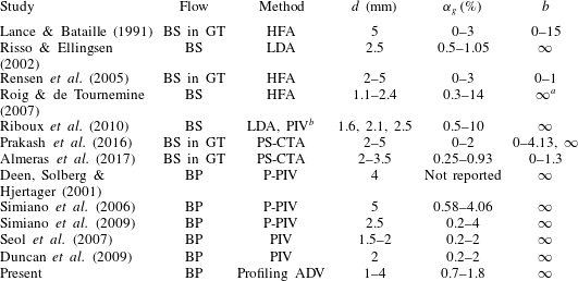
There are two challenges in making liquid velocity measurements in bubbly flows. The first is to distinguish between liquid- and bubble-phase velocities. The second is to measure the induced liquid turbulence with sufficient spatial-temporal resolution. We summarize in table 1 the experimental conditions of previous studies on vertical bubbly flows. The included studies all investigated the liquid flows created by millimetre-sized bubbles and by dilute to moderate void fractions. Hot-film (wire) anemometry (HFA) was often used in early studies. Its working principles and required signal processing for the identification of bubble spikes are described in detail in Rensen, Luther & Lohse (Reference Rensen, Luther and Lohse2005). Phase-sensitive, constant-temperature anemometry (PS-CTA) was developed by the same research group at the University of Twente (Prakash et al.
Reference Prakash, Mercado, van Wijngaarden, Mancilla, Tagawa, Lohse and Sun2016; Almeras et al.
Reference Almeras, Mathai, Lohse and Sun2017). It is essentially the same as HFA with an added optical fibre to detect bubble–probe interactions in situ, thus rendering bubble spike identification by signal processing unnecessary. Both HFA and PS-CTA sample the flow in excess of kilohertz. On the contrary, laser Doppler anemometry (LDA) and particle image velocimetry (PIV) operate in the tens to hundreds hertz range. So, what is the implication of the large difference in temporal sampling frequency on the resolved kinetic energy of the flow? The velocity spectra reported in Prakash et al. (Reference Prakash, Mercado, van Wijngaarden, Mancilla, Tagawa, Lohse and Sun2016) and Almeras et al. (Reference Almeras, Mathai, Lohse and Sun2017) show that the normalized power spectral density decreases monotonically with frequency, decaying by over four orders of magnitude (from
 $10^{0}$
to
 $10^{-4}$
) over the frequency range 1–100 Hz. We conclude from this that virtually all of the kinetic energy created by the rising bubbles can be captured by a sampling frequency of 100 Hz, at least with respect to the present and previous experimental conditions (flow rate and void fraction) reported in table 1.
Summary of the experimental conditions in previous studies on vertical bubbly flows. BS = homogeneous bubble swarm. BP = bubble plume. GT = grid turbulence. HFA = hot-film anemometry. LDA = laser Doppler anemometry. PS-CTA = phase-sensitive constant-temperature anemometry. (P)-PIV = (phase-discriminating)-particle image velocimetry. ADV = acoustic Doppler velocimetry. The bubble Reynolds number
 $Re_{b}=u_{s}d/\unicode[STIX]{x1D708}$
is greater than 400 in all studies; the bubble wakes are fully turbulent.

a
A small coflow was maintained in the vertical water channel to facilitate HFA measurements, and so
 $b$
was not exactly
 $\infty$
.
b LDA was used inside the bubble swarm whereas PIV was used in the wake behind the swarm.
In this study, we have used a different measurement technique than those listed in table 1 and used in previous studies. We apply the Nortek Vectrino II acoustic Doppler velocimeter (ADV) for three-component fluid velocity measurements. The Vectrino II is the latest generation of ADVs and is capable of simultaneous, three-velocity-component measurements at 1 mm increments along a 35 mm strip at temporal frequencies up to 100 Hz and at spatial resolutions from 4 mm down to 1 mm (Nortek 2013). The coherent-pulse technology of ADVs is well understood and its performance in probing energetic turbulent flows is well documented (Voulgaris & Trowbridge Reference Voulgaris and Trowbridge1998). When an ADV is used in a bubbly environment, concern arises on whether the measurements are physical in the presence of air bubbles, which are strong acoustic scatterers. It is commonly believed that bubbles cause non-physical velocity spikes to appear in the time series which have to be removed and replaced by interpolation. Here, we show that all data measured by the Vectrino II are physical within our bubble plumes with air void fractions
 $\unicode[STIX]{x1D6FC}_{g}<2\,\%$
. We make use of this data to study the t.k.e. budget in a bubble plume and to measure the turbulence physics of heterogeneous bubbly swarms.
This paper is organized as follows. The laboratory set-up, experimental conditions and some operational details of the Vectrino II are given in § 2. We examine the empirical probability density functions (PDF) of the three velocity components to show that they agree with those measured in homogeneous bubble swarms in § 3. In § 3, we also quantify the data fraction of bubble wakes, the slip velocity between air and water and the characteristic frequency at which the bubbles inject t.k.e. into the surrounding water. The results of the first, second- and third-order velocity statistics follow in § 4. Using fitted continuous functions derived from these statistics, we derive the t.k.e. budget in the asymptotic plume regime in § 5. We end with a summary of the key findings and general conclusions in § 6.
2 Bubble plume experiments
The experiments were done in the Fluid Dynamics Laboratory in the Zachry Department of Civil Engineering at Texas A&M University. To establish an almost symmetric flow field, a
 $1~\text{m}^{3}$
cube compartment was partitioned from a glass-walled rectangular water tank. A diagram of the experimental set-up is shown in figure 1. Compressed air was injected into the cube through an aquarium airstone (a 14 mm diameter porous cylinder with a 30 mm height) located at the centre of the bottom face; the top of the airstone is 79 mm above the tank floor. The volume inflow rate of air
 $Q_{o}$
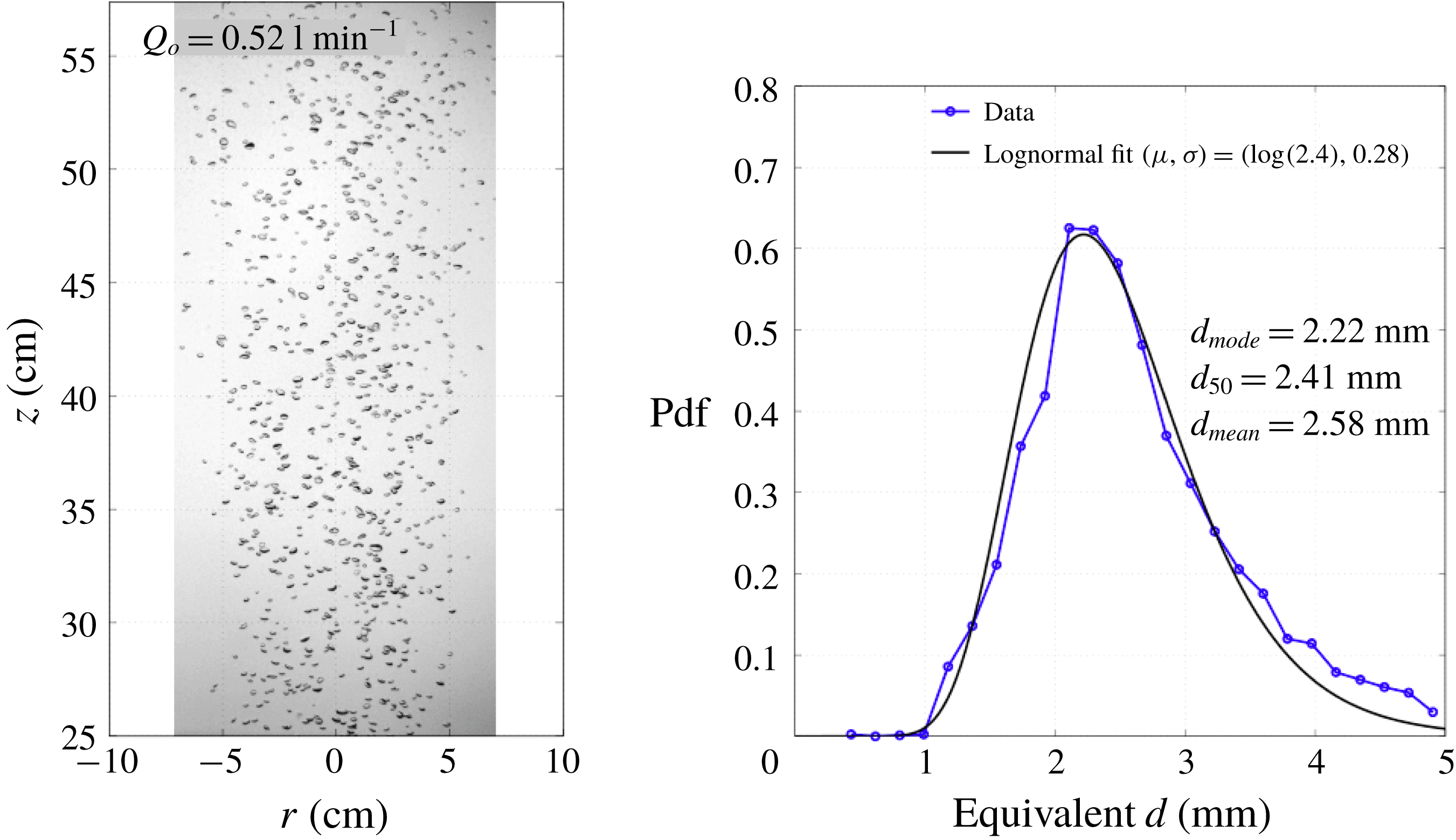
at standard temperature and pressure (STP) was monitored by a calibrated mass-based gas flowmeter (GFM 171, Aalborg Instruments & Controls, Inc.). Air bubbles generated by the airstone had diameters in the range of 1–4 mm and a median diameter
 $d_{50}$
of 2.4 mm (figure 2) with a corresponding slip velocity computed from correlation equations for bubbles of
 $0.24~\text{m}~\text{s}^{-1}$
(Clift, Grace & Weber Reference Clift, Grace and Weber1978). Both Cartesian and cylindrical polar coordinates are used: in the Cartesian system
 $(x,y,z)$
,
 $z$
is the vertical (streamwise) axis,
 $x$
is the horizontal axis of the measurements and
 $y$
is the out-of-plane axis; in the cylindrical polar system
 $(r,\unicode[STIX]{x1D703},z)$
,
 $r$
is the radial coordinate,
 $\unicode[STIX]{x1D703}$
is the horizontal angle measured from the
 $x$
-axis and
 $z$
is the same in both systems. The corresponding instantaneous velocity components are
 $\tilde{w}$
in the
 $z$
-direction,
 $\tilde{u}$
in the
 $x$
- and
 $r$
-directions and
 $\tilde{v}$
in the
 $y$
-direction. The origin of both coordinate systems is the top of the diffuser.
Schematic diagram of the laboratory set-up in present study.

Bubble size distribution for case A.

A Nortek Vectrino II profiler mounted on a motorized linear stage (Zaber Technologies) was used to measure fluid velocities at different source elevations. Data were obtained at 1 mm intervals in the radial direction along a 35 mm long strip. The sample volume is cylindrical with a diameter of 6 mm normal to the strip axis. At each measurement height, twenty-three overlapping strips were used to span the whole bubble plume. The overlap was determined so that only data from cells 6 to 16 (an 11 mm long section of the strip) needed to be stacked to obtain a complete profile. This overlap was chosen to ensure that the most sensitive region of the strip was used to obtain the data. This decision is based on the varying sensitivity of the probe and is discussed in more detail in § 2.1. Each 1 mm thick sampling disc has a sampling volume of
 $9\unicode[STIX]{x03C0}~\text{mm}^{3}$
, which is equivalent to a cube with sides of length 3 mm.
For an ADV, Garcia et al. (Reference Garcia, Cantero, Nino and Garcia2005) showed that if the dimensionless frequency
 $F=f_{s}L/U_{c}>20$
over 90 % of the total t.k.e. is captured, and the energy aliased from frequencies larger than the Nyquist frequency is negligible. Here,
 $f_{s}$
= sampling frequency,
 $L$
= size of energy containing eddies and
 $U_{c}$
= convective velocity. This criterion was satisfied in the present experiments by choosing
 $f_{s}=50$
Hz with
 $L\sim 0.1$
m and
 $U_{c}\sim 0.2~\text{m}~\text{s}^{-1}$
(see table 3). The two-phase bubble plume is known to exhibit large-scale oscillations (Milgram Reference Milgram1983). Using the empirical relationship given in Seol, Duncan & Socolofsky (Reference Seol, Duncan and Socolofsky2009), the wandering period is estimated at 1.5 min for Case A in our tank. Therefore, the plume flow was sampled for 15 min at each measurement strip, which covered approximately ten wandering periods, and a total of 5.75 h was required to complete the 23 overlapping strips at each measurement height. Table 2 shows the experimental conditions and relevant dimensional and non-dimensional quantities.


2.1 Operational details of Nortek Vectrino II
The Vectrino II profiling ADV was introduced by Nortek in 2011 (Craig et al.
Reference Craig, Loadman, Clement, Rusello and Siegel2011). Our work using the instrument in bubbly flows reveals the following. Pulse interference is common because of a tight bubble core, and we enabled the adaptive ping algorithm in the instrument software to eliminate these weak spots. To ensure the highest possible data quality, two precautionary steps were taken in the experiments. First, the water tank was adequately seeded with neutrally buoyant
 $50~\unicode[STIX]{x03BC}\text{m}$
polyamide particles such that the background (without bubble plume flow) signal-to-noise ratio (SNR) and correlation coefficient (Corr) were better than 30 and 98 %, and that their profiles were parabolic with a peak at the sweet spot of the measurement strip (Nortek 2013). Second, a probe check was performed with the plume flow turned on before each experiment run. The amplitude profiles of the four receivers should overlap and be smooth across the measuring strip, and again with a distinct maximum at the strip sweet spot. A schematic sketch of the thirty-five sampling disks is shown in figure 3. The probe’s sweet spot is approximately 5 cm from the transmitter head and corresponds to the tenth cell in the measurement strip. In this study, only data from the sixth to sixteenth cells are considered due to the decaying sensitivity, hence accuracy, at both ends of the strip. These eleven cells were repeatedly used to sample the plume flow at different radial positions. The data quality is discussed in detail in the result section § 4.
Characteristics of the sampling disks of the Vectrino II; showing the varying measurement sensitivity and the positions of data considered in present study.

2.2 Post-processing of raw ADV data
In the ADV community, the term despiking refers to the removal of faulty data in a velocity time series (Goring & Nikora Reference Goring and Nikora2002). Faulty data usually appear as extreme values and are removed by either thresholding on the SNR/Corr values, or more commonly, by statistical methods that better respond to flow physics. In recent literature on despiking, the class of phase-space despiking methods has been suggested as an objective rejection algorithm, first advocated by Goring & Nikora (Reference Goring and Nikora2002). The method is based on a classical statistical result of the normal (Gaussian) distribution: extreme values cannot appear more often than a certain limit. The presumed Gaussian behaviour appears to apply in many turbulent fluid flows although non-Gaussianity of the small dissipative scales is recognized (Pope Reference Pope2000). More importantly, this despiking method assumes that there is only one forcing responsible for the data, which is true for flows characterized by a single length scale, e.g. a single-phase jet. In multiscale flows such as bubble plumes, there can be multiple forcings. Each may have a different PDF and contribute a different data fraction. Blindly despiking such data will lead to the removal of physical data. Cea, Puertas & Pena (Reference Cea, Puertas and Pena2007) recognized the issue and applied a modified phase-space algorithm to a dataset obtained in the highly aerated flow behind a sluice gate. We will show in § 3 that our bubble plume data do not need despiking, and we will demonstrate that the extreme values are signatures of liquid fluctuations created by the rising bubbles.
2.3 Noise-reduced estimates of the Reynolds stress tensor
It is known that raw ADV data obtained from flows without any physical obstructions are accurate for computing the mean flow field while turbulent statistics are highly biased by the Doppler noise which must be estimated and removed from measurements, see e.g. Voulgaris & Trowbridge (Reference Voulgaris and Trowbridge1998) and Garcia et al. (Reference Garcia, Cantero, Nino and Garcia2005). For a four-receiver bistatic probe like the Vectrino II, the redundant (along transmitter direction) radial velocity
 $\tilde{u} 2$
can be used together with
 $\tilde{u} 1$
to directly estimate the Doppler noise. Noise-reduced estimates of the Reynolds stress tensor can then be obtained after accounting for probe geometry (Hurther & Lemmin Reference Hurther and Lemmin2001). Details of the correction procedure are given in appendix A.
3 Characteristics of liquid fluctuations
We first inspect the empirical PDFs of the raw velocities to understand the statistical nature of the velocity fluctuations. This is followed by a comparison with the PDFs measured in homogeneous bubble swarms for
 $b=1.3$
and
 $\infty$
. We then carry out a decomposition of the streamwise velocity
 $\tilde{w}$
PDF into three, superposed Gaussian distributions in order to quantify the data fraction contributed by bubble wakes and to estimate the relative (slip) velocity between bubbles and water. Further, we conduct a wavelet analysis to elucidate the non-stationary characteristics of
 $\tilde{w}$
, and in particular, to determine the characteristic frequency at which bubbles inject kinetic energy into the surrounding liquids.
3.1 Empirical probability density functions
Figure 4 shows a six minute segment (out of a full 15 min record) of the raw streamwise velocity
 $\tilde{w}$
at the plume core
 $r=0$
and at
 $z/D=6.6$
for a single sample volume along the strip for Case A. When viewed over the entire segment, the series is stationary in time but is also interlaced with intermittent large negative and positive values. This means that the series is not locally stationary, i.e. over small time intervals. Fluctuations of much higher frequencies than those present during typical times occur when
 $\tilde{w}$
attains extreme values.
Raw data for streamwise velocity
 $\tilde{w}$
at plume core
 $r=0$
(Case A,
 $z/D=6.6$
).

Empirical PDF of raw velocities at the plume core
 $r=0$
(Case A,
 $z/D=6.6$
): (a) velocities
 $\tilde{w}$
and
 $\tilde{v}$
in the Cartesian reference frame; (b) the two independent measurements
 $\tilde{u} 1$
and
 $\tilde{u} 2$
of the radial velocity.

The corresponding empirical PDFs are shown in figure 5. Two characteristics are observed for
 $\tilde{w}$
: (i) a primary peak at approximately
 $0.18~\text{m}~\text{s}^{-1}$
, characterized by a distribution of positive velocities that is right skewed; and (ii) a broad distribution of negative velocities (mean of all negative values is
 $-0.35~\text{m}~\text{s}^{-1}$
) but having low probability densities. These large negative velocities do not occur due to phase wrapping of the ADV as the same values result when doubling the velocity range of the signal processor. The interpretation of these observations is analysed in detail in § 3.2.
In contrast to the PDF for
 $\tilde{w}$
, the out-of-plane velocity
 $\tilde{v}$
has only one peak in its PDF. The PDF is symmetric with respect to zero velocity, as can be expected from the flow symmetry at the plume core. Similar observations can be found from the PDFs of the radial velocities
 $\tilde{u} 1$
and
 $\tilde{u} 2$
. Hence, the rapid vertical rise of air bubbles created definite signatures in
 $\tilde{w}$
only.
Empirical PDF of the three velocity components at the bubble plume centreline (
 $r=0$
): Case A at
 $z/D=6.6$
(a,b) and Case B at
 $z/D=2.2$
(c,d).

Empirical PDF of the three velocity components at the edge of the bubble plume (
 $r=2b_{g}$
): Case A at
 $z/D=6.6$
(a,b) and Case B at
 $z/D=2.2$
(c,d).

Figures 6 and 7 compare the velocity PDFs of our bubble plumes with those of homogeneous bubble swarms reported in Riboux et al. (Reference Riboux, Risso and Legendre2010), Prakash et al. (Reference Prakash, Mercado, van Wijngaarden, Mancilla, Tagawa, Lohse and Sun2016) and Almeras et al. (Reference Almeras, Mathai, Lohse and Sun2017). In these figures, PDFs of the standardized velocity
 $(\tilde{u} _{i}-U_{i})/u_{i,rms}$
(rms, root-mean-square) are plotted, where
 $i$
is the coordinate axis in indicial notation. This standardization facilitates the comparison among flows with different void fractions, and hence, different magnitudes of kinetic energy of the induced liquid fluctuations. The figures are also plotted with a semi-log ordinate axis to show the stretched exponential tails of the PDFs (Risso Reference Risso2018); PDFs having the form
 $p(x)\sim \exp (-|x|)$
will appear as straight lines in such a plot.
At the bubble plume centreline
 $r=0$
, figure 6 shows that for both Cases A and B the streamwise (vertical) liquid fluctuations have very similar PDFs to those of bubble swarms. All PDFs are positively skewed, and fluctuations over the range
 $2<(\tilde{w}-W)/w_{rms}<6$
have higher occurrence probabilities than that given by the standard Gaussian PDF (black dashed line). In fact, our data almost overlap exactly with the LDA data reported in Riboux et al. (Reference Riboux, Risso and Legendre2010). For the two horizontal velocity components (
 $\tilde{u} ,\tilde{v}$
), the agreement of the PDFs between the bubble plume data and the bubble swarms data (Riboux et al.
Reference Riboux, Risso and Legendre2010) is again very good. Unlike the PDF of
 $\tilde{w}$
, these PDFs are symmetric. Finally, all velocity components exhibit multiple, stretched exponential tails, an observation already reported for bubble swarms (Risso Reference Risso2018). From the comparisons just made, two conclusions on bubble-induced liquid fluctuations can be drawn: (i) rising bubbles create a specific pattern of liquid fluctuations that are insensitive to the details of the flow (e.g. heterogeneity, void fraction and background flow) as seen in the similarities of the PDFs of standardized velocity for these diverse conditions, and (ii) our temporal sampling frequency of 50 Hz was adequate to capture essentially all of the most energetic liquid fluctuations.
To extend our analysis outside the plume core, PDFs of the velocity components at the plume edge
 $r=2b_{g}$
(
 $b_{g}$
is the Gaussian plume radius; details in § 4) are shown in figure 7. At this large radial position, the flow is nearly single phase, except for the rare event of bubbles having drifted away from the core. The flow condition can be likened to bubbly flows with a small bubblance parameter
 $b$
. We therefore choose the data from Prakash et al. (Reference Prakash, Mercado, van Wijngaarden, Mancilla, Tagawa, Lohse and Sun2016) for homogeneous bubble swarms (
 $\unicode[STIX]{x1D6FC}_{g}=0.2\,\%$
) with the smallest
 $b=0.03$
and with bubble diameters in the range
 $d=2{-}4$
mm for comparison with our data. For
 $\tilde{w}$
, the comparison is good. The PDF is much less positively skewed than in the core of our bubble plume and only deviates from the Gaussian PDF for probability densities smaller than
 $10^{-3}$
at the positive tail of the distribution. These deviations with low probabilities of occurrence are associated with the stray bubbles. For the horizontal velocities (
 $\tilde{u} ,\tilde{v}$
), their PDFs conform closely to the Gaussian PDF fit. For all velocity components, the stretched exponential tails observed at the plume centreline no longer exist at the plume edge. The liquid fluctuations are created by the plume entrainment and are modified by the rare passage of rising bubbles.
Evolution of empirical PDF of raw velocities of Case A at
 $z/D=6.6$
and for
 $r=0{-}50~\text{mm}=0{-}0.92b_{g}$
;
 $\tilde{w}$
(a),
 $\tilde{v}$
(b) and
 $\tilde{u}$
(c).

Evolution of empirical PDF of raw velocities of Case A at
 $z/D=6.6$
and for
 $r=55{-}105~\text{mm}=1{-}1.92b_{g}$
;
 $\tilde{w}$
(a),
 $\tilde{v}$
(b) and
 $\tilde{u}$
(c).

The results at the plume centreline (figure 6) and plume edge (figure 7) represent the two limiting cases in the continuous evolution of velocity PDFs as one travels radially outward from the centreline. To illustrate such evolution of the PDFs across the plume, we plot the data from Case A at
 $z/D=6.6$
for the range
 $r=0{-}105~\text{mm}=0{-}1.92b_{g}$
in figures 8 and 9. In these figures, all
 $\tilde{w}$
-PDFs are positively skewed, and a tertiary peak with positive velocity gradually emerges in the
 $\tilde{w}$
-PDFs as
 $r$
increases (see figure 8
a). This tertiary peak in the
 $\tilde{w}$
PDF decays away as
 $r$
continues to increase, disappearing at around
 $r=65$
mm. In contrast, all PDFs of the horizontal velocities (
 $\tilde{u} ,\tilde{v}$
) are symmetric across all
 $r$
. These qualitative observations are also found for all other elevations
 $z/D$
and for Case B. In the next section, we decompose the
 $\tilde{w}$
-PDFs to better understand the origin of the tertiary peaks and of the negative velocities observed in figures 4, 8 and 9.
3.2 Decomposition of streamwise velocity
 $\tilde{w}$

To decompose the
 $\tilde{w}$
-PDFs, we first separate the extreme values of
 $\tilde{w}$
into two groups using a median filter:
 $$\begin{eqnarray}C_{2}\unicode[STIX]{x1D706}~\text{median}(|\tilde{w_{i}}-\text{median}(\tilde{w_{i}})|),\end{eqnarray}$$
where
 $C_{2}=1.35$
,
 $\unicode[STIX]{x1D706}=\sqrt{2\log (N)}$
and
 $N$
= number of data points in a time series (Goring & Nikora Reference Goring and Nikora2002; Cea et al.
Reference Cea, Puertas and Pena2007). This set of constants is applied to all data.
Referring back to figure 5, the median filter identifies extreme values relative to the central primary peak which is assumed to take on a Gaussian shape. We then label the extreme values as follows: those with positive values of
 $\tilde{w}$
are termed the wake (tertiary peak) and those with negative
 $\tilde{w}$
termed the return flow (secondary peak). We also calculate the data fraction
 $n_{i}$
for each of these extreme value components in the full time series. The results for both Cases A and B are shown in figure 10. The radial distance
 $r$
(abscissa) has been normalized by the Gaussian plume radius
 $b_{g}$
(see § 4). For
 $r/b_{g}<1$
, the return flow accounts for less than (
 $n_{1}=\;$
) 2 % of the data; whereas, the wake contributes a significant portion at (
 $n_{3}=\;$
) 5–25 %. As one moves away from
 $r=0$
,
 $n_{3}$
decreases steadily to low values. Previous void fraction measurements for the same diffuser at the same gas flow rates (Seol et al.
Reference Seol, Bhaumik, Bergmann and Socolofsky2007) found that the time-averaged
 $\unicode[STIX]{x1D6FC}_{g}$
is in the range 0.7–1.8 %. This correlates very well with our
 $n_{1}$
and indicates that large negative values of
 $\tilde{w}$
are related to the passage of an air bubble through the ADV sampling volume. Further, the wake fraction
 $n_{3}$
is much larger than that of the return flow because the latter is a very localized process. In their numerical simulations on bubble columns (
 $\unicode[STIX]{x1D6FC}_{g}<4\,\%$
), Riboux et al. (Reference Riboux, Legendre and Risso2013) show that bubble wakes have lengths ten times the bubble diameter. It is therefore reasonable to see a significant wake contribution in excess of the void fraction to the total data signal.
Data fraction identified as return flow
 $n_{1}$
or wake
 $n_{3}$
by the median filter in (3.1).

Through this extreme value analysis, we have shown that the positive tails of the
 $\tilde{w}$
-PDFs correspond to a signature of the bubble wakes. In fact, there are three physical mechanisms creating the velocity fluctuations in
 $\tilde{w}$
: (i) return fluid flow caused by rising bubbles, (ii) bulk entrained fluid in the bubble plume and (iii) bubble wakes. The boundary between contributions from the bulk flow and bubble wakes is not distinct because plume entrainment is a collective result of the bubble wakes. Nonetheless, this classification is useful as the bulk fluid and the bubble wake have different velocities, and we expect that the latter is larger and that the time-averaged velocity difference between these two contributions is close to the slip velocity between the two phases.
For the return flow contribution, we can show that the negative values are a necessity from mass conservation of the liquid fraction. Let us consider the return flow caused by the rise of a single bubble inside a cylinder of diameter
 $D$
in which the ambient fluid is initially motionless. If
 $d$
is the bubble diameter and
 $u_{rise}$
is the bubble rise velocity, then a void volume must be created at a rate equal to
 $(\unicode[STIX]{x03C0}/4)d^{2}u_{rise}$
along the trajectory of the bubble. As this void moves upward in an Eulerian perspective, the void at a position
 $\boldsymbol{x}$
immediately after passage of the bubble must be filled by a downflow of ambient water. The average velocity of this downflow is
 $\overline{u_{d}}=d^{2}u_{rise}/(D^{2}-d^{2})$
which shows that
 $\overline{u_{d}}$
can attain very large values as
 $D\rightarrow d$
. In figure 4, we interpret the large negative velocities as the return flow which have a mean of
 $\overline{u_{d}}=0.35~\text{m}~\text{s}^{-1}$
in this case. The rise velocity
 $u_{rise}$
is
 $0.50~\text{m}~\text{s}^{-1}$
which is the sum of the local bulk fluid velocity (
 ${\sim}0.30~\text{m}~\text{s}^{-1}$
) and slip velocity (Clift et al.
Reference Clift, Grace and Weber1978,
 $0.24~\text{m}~\text{s}^{-1}$
). Using
 $d=d_{50}=2.4$
mm and solving for
 $D$
, we find
 $D=3.6$
mm. The periphery gap
 $D-d$
that allows drainage of the return flow is, thus, a 0.6 mm thick annular ring. This scale is of the same order as the 1 mm radial resolution of the ADV, and therefore, one can expect the return flow be captured in our data.
With these heuristic arguments at hand, we expect that
 $\tilde{w}$
is created by the interaction of all three mechanisms of return flow around bubbles, mean flow of the bubble plume and wake flow behind the bubbles. We hypothesize that each of these features has a Gaussian PDF
 $p_{i}(\tilde{w})$
for which their sum is equal to the total (raw) PDF
 $p_{total}(\tilde{w})$
. We perform a nonlinear curve fitting to calculate the mean and variance of each PDF, i.e. (
 $\unicode[STIX]{x1D707}_{i},\unicode[STIX]{x1D70E}_{i}$
). A constraint that must be satisfied is
 $$\begin{eqnarray}\int _{-\infty }^{\infty }p_{total}(\tilde{w})=\int _{-\infty }^{\infty }(p_{1}(\tilde{w})+p_{2}(\tilde{w})+p_{3}(\tilde{w}))\,\text{d}\tilde{w}=1.\end{eqnarray}$$
To satisfy (3.2), the individual PDF takes the following form
 $$\begin{eqnarray}p_{i}(\tilde{w})=\frac{1}{\sqrt{\unicode[STIX]{x03C0}}}\frac{n_{i}}{\unicode[STIX]{x1D70E}_{i}}\text{e}^{-((\tilde{w}-\unicode[STIX]{x1D707}_{i})/\unicode[STIX]{x1D70E}_{i})^{2}},\end{eqnarray}$$
where
 $n_{i}$
is the data fraction corresponding to mechanism
 $i$
and
 $\sum _{i=1}^{3}n_{i}=1$
.
 $n_{i}$
is calculated from the experimental data by the median filter introduced at the beginning of this section (see also figure 10).
An example of this Gaussian decomposition is shown in figure 11. It can be seen that the total PDF is reasonably fitted by the sum of three Gaussians. Notably, the return flow is well separated from the rest of the flow and the upper end of the bulk entrained fluid flow is indistinguishable from the wake. To substantiate our heuristic arguments, the velocity differential
 $\unicode[STIX]{x0394}\unicode[STIX]{x1D707}=\unicode[STIX]{x1D707}_{3}-\unicode[STIX]{x1D707}_{1}$
, which in principle should correspond to
 $u_{s}$
, is plotted in figure 12 across the plume for both Cases A and B. The radial distance (abscissa) has been normalized by the Gaussian plume radius
 $b_{g}$
(see § 4). At all source elevations
 $z/D$
, a velocity plateau is observed for
 $r/b_{g}<0.8{-}0.9$
. For Case A, this plateau region gives
 $\unicode[STIX]{x0394}\unicode[STIX]{x1D707}=0.20~\text{m}~\text{s}^{-1}$
, and in Case B, the corresponding value is
 $0.20{-}0.25~\text{m}~\text{s}^{-1}$
. The velocity differential then drops off sharply and attains low values beyond
 $r/b_{g}=1$
. We note that value of
 $b_{g}$
in each case increases by 50 % across the measured range
 $z/D$
(see table 4), and the normalization
 $r/b_{g}$
effectively removes the plume growth and collapses the profiles. The values of the velocity plateaus are comparable to the terminal velocity (
 $0.24~\text{m}~\text{s}^{-1}$
) of a single bubble in a quiescent ambient. The observed variations are caused by group effects of bubbles and local state of fluid turbulence, both of which are known to sometimes increase and sometimes decrease the terminal velocity. From the figure, a possible definition of the bubble core radius is
 $b_{b}=0.9b_{g}$
, and this will be used to calculate the bubble column spreading ratio
 $\unicode[STIX]{x1D706}$
in § 4.
Decomposition of the streamwise velocity
 $\tilde{w}$
into the return flow of bubbles, entrained fluid and bubble wake (Case A at
 $z/D=6.6$
,
 $r=0$
).

Velocity differential
 $\unicode[STIX]{x1D707}_{3}-\unicode[STIX]{x1D707}_{1}$
.

Time-averaged slip velocity
 $u_{s}$
between the air- and liquid-phase streamwise velocities reported in the two experimental studies of Deen et al. (Reference Deen, Solberg and Hjertager2001) and Simiano et al. (Reference Simiano, Lakehal, Lance and Yadigaroglu2009). The gas inflow rate in the latter study was
 $Q_{o}=15~\text{l}~\text{min}^{-1}$
and the data were measured at an elevation 438 mm above the source. The inset shows the time-averaged streamwise velocity
 $W$
in normalized coordinates; the solid line represents a Gaussian curve fit to the data. The true slip velocity defined in Simiano et al. (Reference Simiano, Lakehal, Lance and Yadigaroglu2009) is
 $\overline{u_{s}}=\overline{(\tilde{w_{B}}-\tilde{w_{L}})\unicode[STIX]{x1D702}_{B}\unicode[STIX]{x1D702}_{L}}/\overline{\unicode[STIX]{x1D702}_{B}\unicode[STIX]{x1D702}_{L}}$
where
 $\unicode[STIX]{x1D702}_{B}$
and
 $\unicode[STIX]{x1D702}_{L}$
are phase-indicator functions that ensure the slip velocity is only calculated when both phases are present.

Finally, we plot in figure 13 the time-averaged slip velocity
 $u_{s}$
reported in Deen et al. (Reference Deen, Solberg and Hjertager2001) and in Simiano et al. (Reference Simiano, Lakehal, Lance and Yadigaroglu2009). These two experimental studies used phase-discriminating particle image velocimetry (PIV) to measure both air- and liquid-phase velocities. In the figure, we have plotted their data on a normalized
 $r/b_{g}$
-axis, where
 $b_{g}$
is determined from the radial profiles of the time-averaged streamwise velocity
 $W$
(shown in the inset of the figure). Comparing the values of our inferred
 $u_{s}$
shown in figure 12 to the directly measured
 $u_{s}$
in these two studies, we observed that the radial profiles have very similar magnitudes and shapes for
 $r<0.8b_{g}$
. All profiles show the tendency of
 $u_{s}$
to increase from the plume centreline towards the edge at
 $r=b_{g}$
. This is most apparent in the data of Simiano et al. (Reference Simiano, Lakehal, Lance and Yadigaroglu2009) and less so for Deen et al. (Reference Deen, Solberg and Hjertager2001) and for the present data. Beyond
 $r=b_{g}$
,
 $u_{s}$
attained a constant value in both previous studies. The sharp decrease in the values of
 $u_{s}$
observed in the present data can be understood by the fact that we did not directly measure the velocity of bubbles and the low void fraction in this region. As mentioned in the introduction (§ 1), the data in Simiano et al. (Reference Simiano, Lakehal, Lance and Yadigaroglu2009) were taken in the plume acceleration phase whilst the present data were in the classical plume regime. Their data have
 $Q_{o}=15~\text{l}~\text{min}^{-1}$
which is 10- and 30-fold the air inflow rates in Cases B and A, respectively. Although their data were measured at a height (
 $=438$
mm) comparable to our first measurement station at 447 mm above source level, their plume was dynamically very different from ours. Their data have a value of
 $z/D$
of only 0.22 which is much smaller than the
 $z/D=2.2$
and 6.6 for Case B and Case A, respectively. It is then quite remarkable to see the
 $u_{s}$
values determined from both studies are so similar to each other, despite the plumes being so dynamically dissimilar. Overall, we conclude that our inferred slip velocities are consistent with direct measurements that were made in bubble plumes generated under very different experimental conditions.
3.3 Wavelet analysis on streamwise velocity
$\tilde{w}$

To quantify the characteristic frequency at which rising bubbles inject kinetic energy into the surrounding fluid, a wavelet analysis is carried out on the time series of
 $\tilde{w}$
. The wavelet method is widely used to analyse time series with non-stationary statistics (Daubechies Reference Daubechies1990). It is particularly relevant here since the injection of bubble-induced kinetic energy into the bulk plume flow occurs only intermittently in time; the void fraction is at most 2 % inside the plume. Conventional Fourier transform is not applicable for characterizing the rapid and short-lived velocity fluctuations caused by the bubbles because of its poor time localization property (Farge Reference Farge1992). We elect to use the Morlet wavelet in our analysis because of its strengths in decomposing turbulent velocity signals (Farge Reference Farge1992). We employ the continuous wavelet transform and follow the recommendations in Torrence & Compo (Reference Torrence and Compo1998) in choosing the wavelet parameters so that at least 98 % of the energy (variance) in the original time series is captured by the wavelet coefficients. Because the basis functions in the wavelet transform are scaled and shifted versions of a mother wavelet that is not periodic in itself, their scales do not directly correlate with an equivalent Fourier period – which we desire in order to quantify the frequency at which bubbles inject kinetic energy to the flow. It is possible to convert the wavelet scale into its equivalent Fourier period so that one can interpret the results in the usual frequency sense, and this has been reported in Torrence & Compo (Reference Torrence and Compo1998). For a Morlet wavelet, the scale is almost equal to the Fourier period.
Continuous wavelet transform of streamwise velocity
 $\tilde{w}$
using the Morlet wavelet; number of scales analysed = 71, smallest scale
 $s_{o}=2dt=0.04$
s, largest scale
 $J=655$
s.

Figure 14 shows the wavelet results for Case A (
 $z/D=6.6$
) at two locations: (i)
 $r=5~\text{mm}=0.1b_{g}$
(plume interior), and (ii)
 $r=65~\text{mm}=1.2b_{g}$
(plume exterior). In the plume interior, there are many needle-like signatures with high frequencies in the time–frequency plot. These signatures are set against the backdrop of a band of energetic low frequencies that persists throughout the entire time record. By contrast, the plume exterior contains only the low-frequency band. From these difference, we can conclude that the high-frequency signatures in the plume core result from the bubble, which are nearly absent in the plum exterior.
A close-up view at
 $r=5$
mm for times between 230 and 250 s (shown in the same figure) reveals that the needle-like signatures are short-lived patches of high energy content. They span a range of frequencies from 1 to 20 Hz, but many of them have frequencies of approximately 10–15 Hz. The two most energetic patches are indicated by arrows, and these may represent the direct passage of bubbles through the ADV sampling volume, thus leaving behind strong signatures. The Nyquist criterion in our present experiment is
 $50~\text{Hz}/2=25$
Hz, which is approximately two times the frequency of these energetic signatures; hence, the bubble-induced turbulence observed in these wavelet analyses was well captured in our experiments.
In their model of bubble-induced turbulence based on large-scale wake interactions, Riboux et al. (Reference Riboux, Legendre and Risso2013) obtained the scaling relationship,
 $f_{cwi}=0.14u_{s}/d$
, for the frequency
 $f_{cwi}$
at which energy generated by the collective wake instability of a group of rising bubbles is injected into the surrounding fluid. Using present values of
 $u_{s}$
and
 $d$
,
 $f_{cwi}=14$
Hz by this expression, and this value corresponds to that of the short-lived energetic patches in our wavelet analysis. Although the scaling relationship in Riboux et al. (Reference Riboux, Legendre and Risso2013) was developed from homogeneous bubble swarm simulations, the correspondence of this scaling relationship with our data again suggests that the nature of bubble-induced turbulence is insensitive to different flow conditions.
4 Mean flow and turbulence statistics
4.1 Mean flow
The instantaneous velocity vector
 $\tilde{\boldsymbol{u}}(\boldsymbol{x},t)$
is decomposed into a time-averaged part
 $\boldsymbol{U}(\boldsymbol{x})$
and a fluctuating part
 $\boldsymbol{u}(\boldsymbol{x},t)$
, e.g. in the streamwise direction
 $\tilde{w}=W+w$
. Figure 15 shows
 $W$
in normalized ordinates. A Gaussian profile was fitted to the data, and the centreline streamwise velocity
 $W_{c}$
and the Gaussian jet radius
 $b_{g}$
were obtained as a result of the curve fit. In both Cases A and B, the profile
 $W/W_{c}=\text{e}^{-(r/b_{g})^{2}}$
fits the data reasonably well;
 $b_{g}$
is defined as the radial location
 $r$
where
 $W=\text{e}^{-1}W_{c}$
. The discrepancies occurring beyond
 $r\geqslant 1.5b_{g}$
are probably caused by large-scale recirculation cells set up inside the tank by the time-steady plume (Fraga et al.
Reference Fraga, Stoesser, Lai and Socolofsky2016).
Normalized radial profiles of the time-averaged streamwise velocity
 $W$
; a comparison between data in the centre portion of the ADV’s measurement strip (a,b) and the data point at sweet spot (c,d);
 $Q_{o}=0.5~\text{l}~\text{min}^{-1}$
(a,c),
 $Q_{o}=1.5~\text{l}~\text{min}^{-1}$
(b,d).

Comparisons of measured plume centreline velocity
 $W_{c}$
(a), Gaussian plume radius
 $b_{g}$
(b) and liquid-phase volume flux
 $Q$
(c) with published data.

Using dimensional analysis, the time-averaged plume centreline velocity
 $W_{c}(z)$
, Gaussian plume radius
 $b_{g}(z)$
and fluid-phase volume flux
 $Q(z)$
have the following functional dependence (Bombardelli et al.
Reference Bombardelli, Buscaglia, Rehmann, Rincon and Garcia2007),
 $$\begin{eqnarray}\frac{b_{g}(z)}{D}=f_{1}\left(\frac{z}{D}\right),\quad \frac{W_{c}(z)}{u_{s}}=f_{2}\left(\frac{z}{D}\right),\quad \frac{Q(z)}{u_{s}D^{2}}=f_{3}\left(\frac{z}{D}\right).\end{eqnarray}$$
Figure 16 shows comparisons of
 $W_{c}$
,
 $b_{g}$
and the fluid-phase volume flux
 $Q=\unicode[STIX]{x03C0}b_{g}^{2}W_{c}$
with previous experimental data in Seol et al. (Reference Seol, Bhaumik, Bergmann and Socolofsky2007) and datasets compiled in Milgram (Reference Milgram1983). The data compiled in the latter reference were obtained from bubble plumes with much larger scales than ours; the water depth was 50 m, 10 m and 3.66 m in Milgram (Reference Milgram1983), Fannelop & Sjoen (Reference Fannelop and Sjoen1980) and Milgram & Van Houten (Reference Milgram and Van Houten1982), respectively. We fit equations using the functional forms given in (4.1) to our data, and these are presented in the figure as the black, solid lines. Remarkable agreement can be seen between these empirical relationships derived from the present small-scale plumes and previous large-scale plumes. For
 $W_{c}$
, the PIV data in Seol et al. (Reference Seol, Bhaumik, Bergmann and Socolofsky2007) are approximately 20–30 % lower than the empirical fit and other datasets. We expect this is because the wake velocities immediately behind the bubbles were not captured by their PIV technique, leading to underestimated liquid-phase velocities inside the plume core. Earlier studies like that of Milgram (Reference Milgram1983) employed mechanical current meters that had no phase-discrimination problem and so
 $W_{c}$
was probably not underestimated. If it is assume that
 $W$
at the plume edge was only slightly underestimated by Seol et al. (Reference Seol, Bhaumik, Bergmann and Socolofsky2007) due to the low void fraction there, a lower
 $W_{c}$
would probably lead to a larger
 $b_{g}$
. Indeed,
 $b_{g}$
in Seol et al. (Reference Seol, Bhaumik, Bergmann and Socolofsky2007) is 18 % (
 $0.132z$
) larger than the value derived from the present data (
 $0.114z$
). This interpretation is further supported by
 $Q$
; despite the differences in
 $W_{c}$
and
 $b_{g}$
, the data for
 $Q$
agree very well with the empirical fit. Since for dilute plumes,
 $Q=\unicode[STIX]{x03C0}b_{g}^{2}W_{c}$
, if
 $Q$
is to remain the same when
 $b_{g}$
is increased by 20 %,
 $W_{c}$
must decrease by 30 %. This reduction compares very well with their
 $W_{c}$
data. Finally, the steeper decay slope of
 $W_{c}$
found by a numerical and analytical approach in Bombardelli et al. (Reference Bombardelli, Buscaglia, Rehmann, Rincon and Garcia2007) (red solid line in figure 16) is not observed in the combined dataset that spans
 $0.01<z/D<11$
. Further experiments are needed in the range
 $10<z/D<100$
to explore the
 $(z/D)^{-1/2}$
decay suggested in Bombardelli et al. (Reference Bombardelli, Buscaglia, Rehmann, Rincon and Garcia2007).
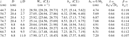
Measured mean flow properties of bubble plumes in present study. C.I. is the 95 % confidence interval of the fitted
 $W_{c}$
and
 $b_{g}$
. The
 $\sqrt{2}$
appearing in
 $\unicode[STIX]{x1D706}$
accounts for the difference between top-hat and Gaussian profile formulation of integral plume models.

Table 3 tabulates the numerical values of various mean flow properties. The bubble core radius
 $b_{b}$
is estimated from figure 12 in the manner described in § 3.2.
 $b_{b}$
is interpreted as a top-hat radius and, thus, a factor of
 $\sqrt{2}$
is multiplied to
 $b_{g}$
when calculating the spread width ratio
 $\unicode[STIX]{x1D706}$
. A value of 0.64 is obtained for
 $\unicode[STIX]{x1D706}$
, which is somewhat smaller than data in Seol et al. (Reference Seol, Bhaumik, Bergmann and Socolofsky2007). The liquid-phase spreading rate
 $\unicode[STIX]{x1D6FD}$
appears to decrease with
 $z/D$
and attains an asymptotic value of 0.11 for
 $z/D>8$
. Overall, our bubble plume data are consistent with other experimental datasets and exhibit the following dependencies on
 $z$
;
 $W_{c}\sim z^{-1/3}$
,
 $b_{g}\sim z$
and
 $Q\sim z^{5/3}$
. Integral properties of bubble plumes are adequately described by the independent parameters
 $u_{s}$
and
 $D$
. As a further comparison, the entrainment coefficient
 $\unicode[STIX]{x1D6FC}$
in the asymptotic regime (
 $z/D>5$
) of a bubble plume can be computed from the integral equation of conservation of fluid volume flux,
 $\text{d}Q/\text{d}z=2\unicode[STIX]{x03C0}b_{g}^{2}W_{c}$
, using the three empirical fits. The coefficient
 $\unicode[STIX]{x1D6FC}$
can be written as,
 $$\begin{eqnarray}\unicode[STIX]{x1D6FC}=\frac{5}{3}\frac{1}{2\unicode[STIX]{x03C0}}\frac{C_{3}}{C_{2}C_{1}}=0.095,\end{eqnarray}$$
where
 $C_{1}=0.114$
,
 $C_{2}=1.6$
and
 $C_{3}=0.065$
are the empirical-fit constants for
 $b_{g}(z)$
,
 $W_{c}(z)$
and
 $Q(z)$
respectively. This value is somewhat larger than the generally accepted value of 0.083 for a single-phase plume (Fischer et al.
Reference Fischer, List, Koh, Brooks and Imberger1979), but it is well within the range of published data. It should be noted that the spreading rate
 $\unicode[STIX]{x1D6FD}$
for a pure plume is equal to
 $(6/5)\unicode[STIX]{x1D6FC}_{p}$
(Lee & Chu Reference Lee and Chu2003, p. 95) by the equivalence of spreading hypothesis and entrainment hypothesis. Finally, the asymptotic plume densimetric Froude number
 $Fr_{p}$
can be computed from
 $Fr_{p}=(1/\sqrt{2})\sqrt{5/4\unicode[STIX]{x1D6FC}_{p}}\unicode[STIX]{x1D706}$
(Lee & Chu Reference Lee and Chu2003, p. 99); the factor of
 $1/\sqrt{2}$
is used to convert jet radius into diameter so that the definition of
 $Fr_{p}$
becomes identical to that in Wuest et al. (Reference Wuest, Brooks and Imboden1992) and Bombardelli et al. (Reference Bombardelli, Buscaglia, Rehmann, Rincon and Garcia2007). Using
 $\unicode[STIX]{x1D706}=0.64$
from our experiments,
 $Fr_{p}$
equals to 1.63, which is in agreement with the suggested value of 1.6 in Wuest et al. (Reference Wuest, Brooks and Imboden1992) and the analytical value of 1.7 in Bombardelli et al. (Reference Bombardelli, Buscaglia, Rehmann, Rincon and Garcia2007).
4.2 Turbulent Reynolds stresses
Before analysing the time-averaged turbulent stresses, we present the raw data for
 $\overline{w^{2}}$
in figure 17. Figure 17(a) shows the raw data at
 $z/D=8$
for Case A. Inside the plume core (
 $r/b_{g}<1$
), the data for
 $\overline{w^{2}}$
are discontinuous across overlapping strips of the ADV profile. This is witnessed by the upward trend along each ADV strip as the data approach the plume centreline (i.e. decreasing
 $r/b_{g}$
). This inconsistency in the data was caused by the varying sensitivity along the ADV profile described in § 2.1: the ADV probe is more accurate at locations closer to the transmitter head, and these locations were located further away from the plume centre in the experiments. In figure 17(b), data points corresponding to only the sweet spot along each measurement strip are shown, and the turbulence intensity profiles appear continuous across the plume width. This behaviour is representative of all other Reynolds stress data in the present experiments. Hence, only the data obtained at the sweet spot along the ADV profile will be used for analysis of the turbulence quantities in this and later subsections.
Raw ADV data on turbulent stresses; raw data (a) and data at sweet spot (b).

Comparison of measured turbulent stresses by ADV and PIV data (Duncan et al. Reference Duncan, Seol and Socolofsky2009) for Case A.

Comparison of measured turbulent stresses by ADV and PIV data (Duncan et al. Reference Duncan, Seol and Socolofsky2009) for Case B.

Normalized radial profiles of turbulent stresses and turbulent kinetic energy
 $k=1/2(\overline{w^{2}}+\overline{u^{2}}+\overline{v^{2}})$
; a double Gaussian profile (4.3) is fitted to the t.k.e. data.

Figure 18 shows the time-averaged turbulent stresses of Case A. All stresses (streamwise, radial and shear) are normalized using the local streamwise mean velocity at each measurement point
 $W$
and the Gaussian half-width
 $b_{g}$
;
 $W$
is used here to facilitate comparison with the PIV data (sampled at 125 Hz) in Duncan et al. (Reference Duncan, Seol and Socolofsky2009). The increasing trend from the plume centre towards the plume edge agrees with the PIV data. In particular, the comparisons on the radial stress
 $\overline{u^{2}}$
and shear stress
 $\overline{wu}$
are good. For the streamwise (vertical) stress
 $\overline{w^{2}}$
, the ADV data are much higher than the PIV data. This difference is caused by the liquid velocities immediately behind bubble wakes that are not captured in the under-resolved PIV data. Two conclusions can be drawn from this comparison: (i) the 15 min sampling time in this study was adequate to obtain converged and repeatable second-order turbulence statistics and (ii) the plume turbulence is highly anisotropic inside the heterogeneous plume core. This strong anisotropy has also been reported in other experimental studies (Deen et al.
Reference Deen, Solberg and Hjertager2001; Simiano et al.
Reference Simiano, Zboray, de Cachard, Lakehal and Yadigaroglu2006, Reference Simiano, Lakehal, Lance and Yadigaroglu2009). The results for Case B are very similar to those in Case A, as seen in figure 19.
In figure 20 we plot the same data as in figures 18 and 19, but normalized by
 $W_{c}$
instead of the local
 $W$
; the out-of-plane stress
 $\overline{v^{2}}$
is also shown. Inside the bubble plume core, anisotropy of the three stresses is strong (figure 20
a,c). The normalized centreline values of
 $\sqrt{\overline{w^{2}}}$
,
 $\sqrt{\overline{v^{2}}}$
and
 $\sqrt{\overline{u^{2}}}$
are 0.38, 0.23 and 0.18, respectively. When compared to single-phase jets and plumes (Wang & Law Reference Wang and Law2002), the two horizontal intensities are comparable (within 10–15 % of their single-phase counterparts); whereas the streamwise (vertical) intensity in the two-phase plume is 1.5–2 times the single-phase value for
 $r/b_{g}<1$
. Both
 $\overline{w^{2}}$
and
 $\overline{v^{2}}$
show a peak around
 $r/b_{g}=0.55$
. Conversely,
 $\overline{u^{2}}$
remains level across the plume core. This feature of
 $\overline{u^{2}}$
is also observed in a high Reynolds number, single-phase jet (
 $Re=1.4\times 10^{5}$
) (Darisse, Lemay & Benaissa Reference Darisse, Lemay and Benaissa2015). Beyond
 $r/b_{g}=1.5$
, the liquid turbulence attains isotropy as the flow at the plume edge is due to plume entrainment. As discussed for figure 7, the flow is single phase at
 $r/b_{g}>1.5$
(except for the rare passage of stray air bubbles), and the PDFs of liquid fluctuations are Gaussian. The off-centre peak in the
 $\overline{v^{2}}$
-profile and the observation that
 $\overline{v^{2}}>\overline{u^{2}}$
warrant more discussion here. In Darisse et al. (Reference Darisse, Lemay and Benaissa2015), the authors explained for a single-phase jet in air that the differences between the two horizontal stresses are caused by velocity events with a large incident angle relative to the jet centreplane, where
 $\overline{u^{2}}$
resides – hence, resulting from the three-dimensionality of turbulence. As a result, the common approximation
 $\overline{v^{2}}\approx \overline{u^{2}}$
is not true, but is a good approximation in single-phase jets, where their ratio is approximately 1.05. In bubble plumes, the three-dimensionality of the flow is expected to be stronger as the millimetre-sized bubbles have strong wakes and exhibit wobbling trajectories as they rise, leading to a larger
 $\overline{v^{2}}/\overline{u^{2}}$
ratio. Within the bubbly plume core (
 $r<b_{g}$
), this ratio is between 1.1 and 1.3 compared to the value 1.05 reported in single-phase jets.
The profiles of normalized turbulent kinetic energy
 $k=(1/2)(\overline{w^{2}}+\overline{u^{2}}+\overline{v^{2}})/W_{c}^{2}$
shown in figure 20 have a peak at
 $r/b_{g}=0.55$
and can be fitted by a double Gaussian profile:
 $$\begin{eqnarray}k(r)=0.18W_{c}^{2}(z)\exp \left(-\frac{(r-0.55b_{g})^{2}}{(0.5b_{g})^{2}}\right)+\exp \left(-\frac{(r+0.55b_{g})^{2}}{(0.5b_{g})^{2}}\right).\end{eqnarray}$$
We also use a double Gaussian profile to curve fit the individual components of the turbulent stresses, and the resulting curve fit equations are given in appendix D.
For comparison, we include in figure 20 the predictions (dashed lines) from Reynolds-averaged Navier–Stokes (RANS) simulations of the plume that neglect the production of t.k.e. by bubbles. The computational details are given in Lai (Reference Lai2015), and we briefly describe the settings below. The simulations were done with the commercial computational fluid dynamics (CFD) software FLUENT (Ansys Inc.). A mixture model was used in which a single set of governing equations was solved for the mass-weighted mixture properties. The continuous liquid phase and the dispersed bubble phase were modelled as two interpenetrating Eulerian fluids. The air volume fraction was considered as a conservative scalar and tracked by a transport equation. The momentum coupling between the two phases was modelled using the Schiller and Naumann dynamic drag law. The standard
 $k{-}\overline{\unicode[STIX]{x1D716}}$
model was used for closure of the liquid phase turbulence. The
 $k$
and
 $\overline{\unicode[STIX]{x1D716}}$
equations were not augmented by additional source or sink terms to account for bubble-induced liquid turbulence (Vaidheeswaran & Hibiki Reference Vaidheeswaran and Hibiki2017). The simulations therefore only include the production by fluid mean shear (Pope Reference Pope2000). We simulated only half of the time-steady plume by virtue of symmetry in a computational domain that was half of our experimental water tank, i.e. 1 m high by 1 m across the plume by 0.5 m binormal to the vertical and lateral coordinates. The simulations were initialized using the gas inflow rates in table 2, and the gas was released into the domain through a 10 mm inlet (velocity inflow boundary) at the bottom face of the domain. For simplicity, we considered monodisperse bubbles with a median diameter
 $d_{50}=2.4$
mm, matching that of our experiments. The
 $k{-}\overline{\unicode[STIX]{x1D716}}$
model with its standard coefficients do not yield satisfactory predictions of the mean flow quantities
 $W_{c},\unicode[STIX]{x1D6FD}$
and
 $\unicode[STIX]{x1D706}$
. Hence, we adjusted the eddy viscosity coefficient
 $C_{\unicode[STIX]{x1D707}}$
and the turbulent Schmidt number
 $\unicode[STIX]{x1D70E}$
from their standard values, 0.09 and 0.75, to 0.15 and 0.1, respectively, in order to match the experimental results in Seol et al. (Reference Seol, Bhaumik, Bergmann and Socolofsky2007). All other model coefficients retained their standard values. Comparing the predicted and measured
 $k$
, both exhibit an off-centre peak at
 $r/b_{g}=0.5$
. The predictions are, however, only 50–70 % of the measured values inside the plume core. Beyond the core,
 $r/b_{g}>1$
, the two become comparable in magnitude. The comparison, thus, reveals that: (i) while calibration of the closure model coefficients can predict the mean flow, the predictions are correct for the wrong reason – the model neglects the bubble-induced turbulence; and (ii) the t.k.e. injected by bubbles into the liquid is non-negligible.
An example where the t.k.e. production by bubbles is partly accounted for is in the momentum amplification factor
 $\unicode[STIX]{x1D6FE}$
used in integral plume models (Socolofsky et al.
Reference Socolofsky, Bhaumik and Seol2008). We evaluate
 $\unicode[STIX]{x1D6FE}$
using our measured turbulent stresses;
 $\unicode[STIX]{x1D6FE}$
accounts for the kinematic momentum flux carried by the plume turbulence in the model formulation, and it is defined by
 $\unicode[STIX]{x1D6FE}=(\overline{M}+M_{t})/\overline{M}$
, where
 $\overline{M}=2\unicode[STIX]{x03C0}\int _{0}^{\infty }rW^{2}\,\text{d}r$
is the mean momentum flux and
 $M_{t}=2\unicode[STIX]{x03C0}\int _{0}^{\infty }r(\overline{w^{2}}-(1/2)(\overline{u^{2}}+\overline{v^{2}}))\,\text{d}r$
is the momentum flux carried by turbulence. These expressions follow from the boundary-layer approximation to the governing equations of the plume (Lee & Chu Reference Lee and Chu2003). For single-phase jets and plumes
 $\unicode[STIX]{x1D6FE}$
is approximately 1.1 (Wang & Law Reference Wang and Law2002). For bubble plumes, Milgram (Reference Milgram1983) reported values in the range of 1–3. Using the double-Gaussian curve fits for the three normal stresses reported in appendix D,
 $M_{t}=C[0.22-(1/2)(0.097+0.035)]b_{g}^{2}W_{c}^{2}$
where
 $C=2\unicode[STIX]{x03C0}\int _{0}^{\infty }(r/b_{g})G(r/b_{g})d(r/b_{g})=6.1262$
is a shape factor. Together with
 $\overline{M}=(\unicode[STIX]{x03C0}/2)b_{g}^{2}W_{c}^{2}$
, we obtain
 $\unicode[STIX]{x1D6FE}=(0.943+\unicode[STIX]{x03C0}/2)/(\unicode[STIX]{x03C0}/2)=1.6$
in Case A at
 $z/D=8$
. If the variability of the data points used in the curve fit of
 $k$
is accounted for (see figure 20),
 $\unicode[STIX]{x1D6FE}$
is in the range 1.4–1.6. A similar analysis done for Case B yields
 $\unicode[STIX]{x1D6FE}$
in the range 1.45–1.55. The fact that two-phase plumes have larger
 $\unicode[STIX]{x1D6FE}$
values reflects their stronger turbulence anisotropy compared to single-phase jets/plumes.
Finally, some insight on the magnitude of the t.k.e. generated by the bubbles can be extracted from a recent simulation of Case A using a large-eddy simulation (LES) code in Fraga et al. (Reference Fraga, Stoesser, Lai and Socolofsky2016). An Eulerian–Lagrangian approach was used to predict the bubble plume dynamics. The Smagorinsky subgrid-scale (SGS) model with a constant coefficient of 0.1 was used to model the unresolved fluid turbulence. The LES code has been previously verified to produce accurate results in complex geometries, including open-channel flows over a rough bed, compound channel flow, vegetated flows and transport and deposition of fine sediments in open channels (Fraga et al.
Reference Fraga, Stoesser, Lai and Socolofsky2016). The model performs very well for prediction of
 $W_{c}$
,
 $\sqrt{\overline{u^{2}}}$
and
 $\overline{wu}$
; however, the model under-predicts
 $\sqrt{\overline{w^{2}}}$
for
 $r/b_{g}<1$
by up to a factor of two. This difference is because the thin boundary layers around the bubbles were not resolved in the simulation. This motivates us to quantify the t.k.e. production by bubbles.
4.3 Conservation of the total plume momentum flux
Using the mean streamwise velocity
 $W$
and the turbulent Reynolds stresses
 $R_{ii}$
, we assess in figure 21 the conservation of the total plume kinematic momentum flux
 $M$
.
 $M$
has two contributions and is equal to
 $\overline{M}+M_{t}$
:
 $\overline{M}=2\unicode[STIX]{x03C0}\int _{0}^{\infty }rW^{2}\,\text{d}r$
is the mean momentum flux carried by the mean flow;
 $M_{t}=2\unicode[STIX]{x03C0}\int _{0}^{\infty }r(\overline{w^{2}}-(1/2)(\overline{u^{2}}+\overline{v^{2}}))\,\text{d}r$
is the turbulent momentum flux carried by the turbulence (Wang & Law Reference Wang and Law2002; Lee & Chu Reference Lee and Chu2003). The analytical prediction of
 $M$
as a function of
 $z$
for a pure vertical plume is given by (Lee & Chu Reference Lee and Chu2003, p. 83),
 $$\begin{eqnarray}M=(3\sqrt{\unicode[STIX]{x03C0}}\unicode[STIX]{x1D6FD}_{tophat}/4)^{2/3}F_{o}^{2/3}z^{4/3}\approx 0.36F_{o}^{2/3}z^{4/3},\end{eqnarray}$$
where
 $\unicode[STIX]{x1D6FD}_{tophat}=\sqrt{2}\unicode[STIX]{x1D6FD}$
is the top-hat spreading rate, and
 $F_{o}=Q_{o}g$
is the kinematic buoyancy flux exerted by the air bubbles on the surrounding water. Previous experimental studies on single-phase plumes have found the proportionality constant to be 0.29 (Papanicolaou & List Reference Papanicolaou and List1988), 0.34 (Shabbir & George Reference Shabbir and George1994) and 0.38 (Wang & Law Reference Wang and Law2002).
Using the values of
 $Q_{o}$
in table 2 and the average (over the four
 $z/D$
elevations in each case)
 $\unicode[STIX]{x1D6FD}=0.114$
and 0.117 for Cases A and B, the predicted
 $M$
for Cases A and B is plotted as a solid line and a dashed line in figure 21(a), respectively. In physical units, the agreement between the analytical predictions and measurements is very good; the deviations are within
 $\pm 10\,\%$
. The measured data exhibit the expected
 $4/3$
power law with
 $z$
. In figure 21(b), we plot the non-dimensionalized total momentum flux
 $M/(u_{s}D)^{2}$
as a function of
 $z/D$
. The non-dimensionalization effectively collapses the data from both cases onto a single curve. This reinforces the choice of
 $u_{s}$
and
 $D$
as the two governing parameters for dilute bubble plumes. We conclude that our bubble plumes obey the scaling law for momentum conservation in single-phase plumes (
 $M\sim z^{4/3}$
) and that our experimental data are in agreement with the law of conservation of momentum over the range of heights measured here (
 $2<z/D<12$
).
Comparison of measured plume total kinematic momentum flux
 $M=\overline{M}+M_{t}$
and the analytical prediction
 $M=(3\sqrt{\unicode[STIX]{x03C0}}\unicode[STIX]{x1D6FD}_{tophat}/4)^{2/3}F_{o}^{2/3}z^{4/3}$
(Lee & Chu Reference Lee and Chu2003):
 $\unicode[STIX]{x1D6FD}_{tophat}=\sqrt{2}\unicode[STIX]{x1D6FD}$
is the top-hat spreading rate;
 $F_{o}=Q_{o}g$
is the kinematic buoyancy flux exerted by the air bubbles to the liquid. (a) In physical space. (b) In non-dimensional space;
 $C_{4}=(4\unicode[STIX]{x03C0}\unicode[STIX]{x1D6FC}^{2})^{2/3}(3\sqrt{\unicode[STIX]{x03C0}}\unicode[STIX]{x1D6FD}_{tophat}/4)^{2/3}=\unicode[STIX]{x03C0}(3\unicode[STIX]{x1D6FC}^{2}\unicode[STIX]{x1D6FD}_{tophat})^{2/3}$
.

4.4 Triple velocity correlation – turbulent transport of components of t.k.e.
The normalized triple velocity correlations
 $\overline{wu_{i}^{2}}/W_{c}^{3}$
and
 $\overline{uu_{i}^{2}}/W_{c}^{3}$
are shown in figures 22 and 23. In these figures, a correction for Doppler noise is possible in theory, but here this correction was not made because the skewness factor
 $\overline{\unicode[STIX]{x1D70E}_{D}^{3}}$
could not be estimated (see appendix A). Except for the component
 $\overline{uv^{2}}$
(figure 23
c,f), all other components exhibit a reasonable collapse of the data to a single curve for each term when they are normalized by
 $W_{c}^{3}$
and
 $b_{g}$
. For the three axial components
 $\overline{wu_{i}^{2}}/W_{c}^{3}$
, the profile shapes and magnitudes are dissimilar between Cases A and B (see figure 22). This may be explained by their different void fractions: Case B has three times the
 $Q_{o}$
of Case A. On the contrary, the three radial components have similar profiles in both cases (see figure 23).
Normalized radial profiles of axial turbulent
 $\overline{wu_{i}^{2}}$
transport of t.k.e. Different symbols represent data measured at different elevations above source; 44.7 cm, ○ –; 54.7 cm, ▵ –; 64.7 cm, ♢ – and 74.7 cm, ▫ –. The black solid lines are curve fits to the data.

Normalized radial profiles of radial turbulent
 $\overline{uu_{i}^{2}}$
transport of t.k.e. Different symbols represent data measured at different elevations above source; 44.7 cm, ○ –; 54.7 cm, ▵ –; 64.7 cm, ♢ – and 74.7 cm, ▫–. The black solid lines are curve fits to the data. The magenta solid lines are data for a high Reynolds number, single-phase pure jet reported in Darisse et al. (Reference Darisse, Lemay and Benaissa2015). Note that the
 $\overline{uw^{2}}$
jet data have been multiplied by 5 to facilitate the comparison with the corresponding data of the bubble plume.

For comparison, the data of a high Reynolds number, single-phase pure jet reported in Darisse et al. (Reference Darisse, Lemay and Benaissa2015) are included in the plots of figure 23 (solid magenta lines) to highlight this similarity. The
 $\overline{uw^{2}}/W_{c}^{3}$
from the jet data have been multiplied by five to facilitate a comparison of the profile shape. These data comparisons show that
 $\overline{uw^{2}}/W_{c}^{3}$
is negative close to the centreline axis of a jet or bubble plume, becoming positive outside the core, and
 $\overline{u^{3}}/W_{c}^{3}$
is positive across the whole jet or bubble plume. We note that the signs will change on the
 $-r/b_{g}$
axis because of axisymmetry (Darisse et al.
Reference Darisse, Lemay and Benaissa2015). The component
 $\overline{uv^{2}}$
fails to converge in the present experiments inside the bubble core
 $r/b_{g}<1$
. This may be caused by the weak correlation between the plume entrainment flow
 $u$
and the out-of-plane oscillatory liquid motions
 $v$
caused by the bubbles; apparently a much longer sampling time is required to produce converged statistics. Outside the core,
 $\overline{uv^{2}}$
is similar to
 $\overline{uu^{2}}$
, suggesting a similar radial transport. Overall, the results indicate that transport of t.k.e. by the entrainment velocity fluctuations
 $u$
is not sensitive to void fraction; whereas, transport by
 $w$
is sensitive to gas flow rate and, hence, void fraction.
For the purpose of computing the t.k.e. budget, we fit curves to the radial profiles of the turbulent transport components
 $\overline{wu_{i}^{2}}/W_{c}^{3}$
and
 $\overline{uu_{i}^{2}}/W_{c}^{3}$
in the form
 $$\begin{eqnarray}P_{k}(r/b_{g})\exp (-C(r/b_{g})^{2}),\end{eqnarray}$$
where
 $P_{k}(r/b_{g})$
is a polynomial of degree
 $k$
, and
 $C$
is a constant. This choice follows the experimental study on single-phase jets in Hussein, Capp & George (Reference Hussein, Capp and George1994), and the full expressions of each curve fit are given in appendix D. Because the
 $\overline{uv^{2}}$
data fail to converge, we approximate
 $\overline{uv^{2}}$
by
 $\overline{u^{3}}$
. All profiles are practically zero beyond
 $1.2b_{g}$
, indicating that the turbulent transport of t.k.e. is confined within the plume core. This is quite different from a single-phase jet where the profiles extend to
 $r=2b_{g}$
(Darisse et al.
Reference Darisse, Lemay and Benaissa2015).
4.5 Turbulent dissipation rate estimates
We calculate the mean liquid dissipation via the pseudo-dissipation expression
 $\overline{\unicode[STIX]{x1D716}}=\unicode[STIX]{x1D708}\overline{(\unicode[STIX]{x2202}u_{i}/\unicode[STIX]{x2202}x_{j})(\unicode[STIX]{x2202}u_{i}/\unicode[STIX]{x2202}x_{j})}$
, where
 $\unicode[STIX]{x1D708}=0.935\times 10^{-6}~\text{m}^{2}~\text{s}^{-1}$
is the kinematic viscosity of water at
 $23\,^{\circ }\text{C}$
(the temperature in the experiments). The difference between pseudo-dissipation and the true dissipation rate (stress power) is small in high Reynolds number turbulent flows (Pope Reference Pope2000). The full expression of
 $\overline{\unicode[STIX]{x1D716}}$
is:
 $$\begin{eqnarray}\displaystyle \overline{\unicode[STIX]{x1D716}}_{full} & = & \displaystyle \unicode[STIX]{x1D708}\left[\overline{\left(\frac{\unicode[STIX]{x2202}u_{1}}{\unicode[STIX]{x2202}x_{1}}\right)^{2}}+\overline{\left(\frac{\unicode[STIX]{x2202}u_{2}}{\unicode[STIX]{x2202}x_{2}}\right)^{2}}+\overline{\left(\frac{\unicode[STIX]{x2202}u_{3}}{\unicode[STIX]{x2202}x_{3}}\right)^{2}}+\overline{\left(\frac{\unicode[STIX]{x2202}u_{1}}{\unicode[STIX]{x2202}x_{2}}\right)^{2}}+\overline{\left(\frac{\unicode[STIX]{x2202}u_{1}}{\unicode[STIX]{x2202}x_{3}}\right)^{2}}+\overline{\left(\frac{\unicode[STIX]{x2202}u_{2}}{\unicode[STIX]{x2202}x_{1}}\right)^{2}}\right.\nonumber\\ \displaystyle & & \displaystyle +\left.\overline{\left(\frac{\unicode[STIX]{x2202}u_{2}}{\unicode[STIX]{x2202}x_{3}}\right)^{2}}+\overline{\left(\frac{\unicode[STIX]{x2202}u_{3}}{\unicode[STIX]{x2202}x_{1}}\right)^{2}}+\overline{\left(\frac{\unicode[STIX]{x2202}u_{3}}{\unicode[STIX]{x2202}x_{2}}\right)^{2}}\right],\end{eqnarray}$$
where
 $(u_{1},u_{2},u_{3})=(w,u,v)$
and
 $(x_{1},x_{2},x_{3})=(z,x~\text{or}~r,y)$
. We can directly calculate the mean-square radial gradients
 $\overline{(\unicode[STIX]{x2202}u_{1}/\unicode[STIX]{x2202}x_{2})^{2}}$
,
 $\overline{(\unicode[STIX]{x2202}u_{2}/\unicode[STIX]{x2202}x_{2})^{2}}$
and
 $\overline{(\unicode[STIX]{x2202}u_{3}/\unicode[STIX]{x2202}x_{2})^{2}}$
from the data. For the streamwise mean-square gradients
 $\overline{(\unicode[STIX]{x2202}u_{i}/\unicode[STIX]{x2202}x_{1})^{2}}$
, we calculate them indirectly from the temporal data via the modified Taylor hypothesis (Heskestad Reference Heskestad1965):
 $$\begin{eqnarray}\displaystyle \overline{\left(\frac{\unicode[STIX]{x2202}u_{i}}{\unicode[STIX]{x2202}x_{1}}\right)^{2}}=\frac{1}{W^{2}}\overline{\left(\frac{\unicode[STIX]{x2202}u_{i}}{\unicode[STIX]{x2202}t}\right)^{2}}K^{-1}. & & \displaystyle\end{eqnarray}$$
The scalar coefficient
 $K\geqslant 1$
is dependent on the local turbulence intensities and the ratios of the mean-square gradients. The original Taylor hypothesis is recovered when
 $K=1$
. Finally, the unavailable out-of-plane mean-square gradients
 $\overline{(\unicode[STIX]{x2202}u_{i}/\unicode[STIX]{x2202}x_{3})^{2}}$
are replaced by
 $\overline{(\unicode[STIX]{x2202}u_{i}/\unicode[STIX]{x2202}x_{2})^{2}}$
.
For comparison, we also evaluate
 $\overline{\unicode[STIX]{x1D716}}$
with the local isotropy assumption (Taylor Reference Taylor1935) and with the local axisymmetry assumption (George & Hussein Reference George and Hussein1991):
 $$\begin{eqnarray}\displaystyle & \displaystyle \overline{\unicode[STIX]{x1D716}}_{iso}=15\unicode[STIX]{x1D708}\overline{\left(\frac{\unicode[STIX]{x2202}u_{1}}{\unicode[STIX]{x2202}x_{1}}\right)^{2}}=7.5\unicode[STIX]{x1D708}\overline{\left(\frac{\unicode[STIX]{x2202}u_{1}}{\unicode[STIX]{x2202}x_{2}}\right)^{2}} & \displaystyle\end{eqnarray}$$
 $$\begin{eqnarray}\displaystyle & \displaystyle \overline{\unicode[STIX]{x1D716}}_{axi}=\unicode[STIX]{x1D708}\left[\frac{5}{3}\overline{\left(\frac{\unicode[STIX]{x2202}u_{1}}{\unicode[STIX]{x2202}x_{1}}\right)^{2}}+2\overline{\left(\frac{\unicode[STIX]{x2202}u_{1}}{\unicode[STIX]{x2202}x_{2}}\right)^{2}}+2\overline{\left(\frac{\unicode[STIX]{x2202}u_{2}}{\unicode[STIX]{x2202}x_{1}}\right)^{2}}+\frac{8}{3}\overline{\left(\frac{\unicode[STIX]{x2202}u_{3}}{\unicode[STIX]{x2202}x_{2}}\right)^{2}}\right]. & \displaystyle\end{eqnarray}$$
In both (4.8) and (4.9), all terms can be computed from the data either directly, for
 $\overline{(\unicode[STIX]{x2202}u_{i}/\unicode[STIX]{x2202}x_{2})^{2}}$
, or indirectly via Taylor’s hypothesis, for
 $\overline{(\unicode[STIX]{x2202}u_{i}/\unicode[STIX]{x2202}x_{1})^{2}}$
so that there is no need to approximate unavailable out-of-plane gradients. For
 $\overline{\unicode[STIX]{x1D716}}_{iso}$
, we also use
 $\overline{(\unicode[STIX]{x2202}u_{1}/\unicode[STIX]{x2202}x_{2})^{2}}$
in the calculation because it can be directly computed from the data. The required gradients are computed by finite difference and the details are explained in appendix B. The effects of finite spatial resolution on the computed gradients are assessed in appendix C.
Time-averaged normalized mean-square gradients for Case A. Different symbols represent data measured at different elevations above source; 44.7 cm, ○ –; 54.7 cm, ▵ –; 64.7 cm, ♢ – and 74.7 cm, ▫ –.

Figure 24 plots the radial profiles of the mean-square gradients (normalized by
 $(W_{c}/b_{g})^{2}$
) for Case A. Inside the bubbly core (
 $|r/b_{g}|\leqslant 1$
), the radial mean-square gradients, except for
 $\overline{(\unicode[STIX]{x2202}u/\unicode[STIX]{x2202}r)^{2}}$
, are an order of magnitude larger than the streamwise mean-square gradients, and the ratios of the gradients satisfy neither local isotropy nor local axisymmetry assumptions, e.g.
 $2\overline{(\unicode[STIX]{x2202}w/\unicode[STIX]{x2202}z)^{2}}\neq \overline{(\unicode[STIX]{x2202}w/\unicode[STIX]{x2202}r)^{2}}$
and
 $\overline{(\unicode[STIX]{x2202}u/\unicode[STIX]{x2202}x)^{2}}\neq \overline{(\unicode[STIX]{x2202}v/\unicode[STIX]{x2202}x)^{2}}$
. Of the six measurable gradients,
 $\overline{(\unicode[STIX]{x2202}w/\unicode[STIX]{x2202}r)^{2}}$
is the largest. This can be interpreted as connected to the highly dissipative, thin boundary layer around the bubbles (Santarelli et al.
Reference Santarelli, Roussel and Frohlich2016): over a radial distance of the order of the bubble diameter or less, the instantaneous streamwise velocity
 $\tilde{w}$
has to transit from a value close to the bubble rise velocity to a value corresponding to the much lower background plume flow. The streamwise counterpart to
 $\overline{(\unicode[STIX]{x2202}w/\unicode[STIX]{x2202}r)^{2}}$
, given by
 $\overline{(\unicode[STIX]{x2202}w/\unicode[STIX]{x2202}z)^{2}}$
, is small and has only one tenth the magnitude of the radial term. This is expected because the wake region behind each bubble is much longer in length than it is wide (Risso Reference Risso2018). Outside the bubbly core, the mean-square gradients tend to a state of local isotropy, e.g.
 $2\overline{(\unicode[STIX]{x2202}u/\unicode[STIX]{x2202}r)^{2}}\sim \overline{(\unicode[STIX]{x2202}w/\unicode[STIX]{x2202}r)^{2}}\approx \overline{(\unicode[STIX]{x2202}v/\unicode[STIX]{x2202}r)^{2}}\approx \overline{(\unicode[STIX]{x2202}u/\unicode[STIX]{x2202}z)^{2}}$
(Taylor Reference Taylor1935). Together with the t.k.e. (figure 20), this result demonstrates that the boundary-layer flow in the single-phase region of the bubble plume is largely isotropic. The results for Case B (not shown) are similar.
Time-averaged dissipation rate
 $\overline{\unicode[STIX]{x1D716}}$
. Different symbols represent data measured at different elevations above source; 44.7 cm, ○ –; 54.7 cm, ▵ –; 64.7 cm, ♢ – and 74.7 cm, ▫ –.

Figure 25 depicts the normalized dissipation rate profiles for both cases. From these data we find that
 $\overline{\unicode[STIX]{x1D716}}_{axi}\approx \overline{\unicode[STIX]{x1D716}}_{full}$
, that
 $\overline{\unicode[STIX]{x1D716}}_{iso}=15\unicode[STIX]{x1D708}\overline{(\unicode[STIX]{x2202}w/\unicode[STIX]{x2202}z)^{2}}$
under-predicts the dissipation inside the bubbly core, while
 $\overline{\unicode[STIX]{x1D716}}_{iso}=7.5\unicode[STIX]{x1D708}\overline{(\unicode[STIX]{x2202}w/\unicode[STIX]{x2202}r)^{2}}$
over-predicts it, and that all expressions for the dissipation produce similar results outside the bubbly core. It is fortuitous that
 $\overline{\unicode[STIX]{x1D716}}_{axi}\approx \overline{\unicode[STIX]{x1D716}}_{full}$
as we have shown in figure 24 that the mean-square gradients do not satisfy the local axisymmetry relations (George & Hussein Reference George and Hussein1991). Moreover, the behaviour inside the bubble core once again highlights the highly anisotropic nature of the flow in this region.
4.5.1 Conservation of total kinetic energy
Dissipation rate estimates derived from physical experiments commonly suffer from errors due to insufficient spatial resolution and instrument noise; we have implemented the correction method in Hurther & Lemmin (Reference Hurther and Lemmin2001) to reduce the latter’s influence on the results (see appendix A). However, these two sources of error are difficult to disentangle in real experiments in which the true value of
 $\overline{\unicode[STIX]{x1D716}}$
is unknown and in which the adjustment of experimental parameters can reduce one source of error but augment the other.
Here, we assess the accuracy of our estimates of
 $\overline{\unicode[STIX]{x1D716}}$
by carrying out a total kinetic energy balance of the bulk plume flow. This balance equation is obtained from the sum of the transport equations for the mean kinetic energy
 $K=(1/2)(W^{2}+U^{2}+V^{2})\approx (1/2)W^{2}$
(where we have used
 $W\gg U,V$
in jets and bubble plumes) and the t.k.e.
 $k=(1/2)(\overline{w^{2}}+\overline{u^{2}}+\overline{v^{2}})$
(Pope Reference Pope2000, pp. 125–126). In Lai (Reference Lai2015), the equation for
 $K+k$
has been further developed for axisymmetric jets and plumes under the integral framework (Lee & Chu Reference Lee and Chu2003). In essence, the computation of the total kinetic energy balance is to evaluate
 $$\begin{eqnarray}\frac{\text{D}\langle K+k\rangle }{\text{D}t}=-\langle \overline{\unicode[STIX]{x1D716}}\rangle +\langle Wg^{\prime }\rangle ,\end{eqnarray}$$
where
 $\langle \cdot \rangle =2\unicode[STIX]{x03C0}\int _{0}^{\infty }r\,\text{d}r$
denotes a volume average, and
 $g^{\prime }=(\unicode[STIX]{x0394}\unicode[STIX]{x1D70C}/\unicode[STIX]{x1D70C}_{ref})g\approx g=9.81~\text{m}~\text{s}^{-2}$
is the reduced gravity for air bubbles in water.
By the Gauss divergence theorem, the volume averaging removes the gradient flux terms that only redistribute kinetic energy in space by pressure–velocity correlations and by viscous diffusion. Because we only measured at discrete plume elevations, we integrate the volume-averaged total kinetic energy equation in the streamwise direction
 $z$
. This gives the following equation for steady bubble plumes:
 $$\begin{eqnarray}\overbrace{\left({\textstyle \frac{1}{2}}I_{1}+C_{I_{2}}I_{2}\right)[b_{g}^{2}(z)W_{c}^{3}(z)]_{z_{1}}^{z_{2}}}^{\int (\text{D}\langle K+k\rangle /\text{D}t)\,\text{d}z\approx \int _{z_{1}}^{z_{2}}(\unicode[STIX]{x2202}\langle W(K+k)\rangle /\unicode[STIX]{x2202}z)\,\text{d}z}=\overbrace{-{\textstyle \frac{1}{2}}[\langle \overline{\unicode[STIX]{x1D716}}(z_{1})\rangle +\langle \overline{\unicode[STIX]{x1D716}}(z_{2})\rangle ]\unicode[STIX]{x0394}z}^{-\int _{z_{1}}^{z_{2}}\langle \overline{\unicode[STIX]{x1D716}}\rangle \,\text{d}z}+\overbrace{1.36F_{o}\unicode[STIX]{x0394}z}^{\int _{z_{1}}^{z_{2}}\langle wg\rangle \,\text{d}z}.\end{eqnarray}$$
In (4.11),
 $z_{1}$
and
 $z_{2}$
(
 $z_{2}>z_{1}$
) are elevations above the air source, and
 $\langle \overline{\unicode[STIX]{x1D716}}(z)\rangle =b_{g}(z)W_{c}^{3}(z)(C_{I_{3}}I_{3})$
; we have approximated the integral
 $-\int _{z_{1}}^{z_{2}}\langle \overline{\unicode[STIX]{x1D716}}\rangle \,\text{d}z$
by the average of the dissipation measured at
 $z_{1}$
and
 $z_{2}$
:
 $F_{o}=Q_{o}g$
is the kinematic buoyancy flux due to air injection at the source. The constant factor 1.36 accounts for a narrower bubble core than the streamwise fluid velocity profile. Equation (4.11) is a statement of total kinetic energy balance of a conical control volume bounded by any two elevations. For the results presented below, we consider control volumes formed by any two consecutive elevations, leading to
 $\unicode[STIX]{x0394}z=10$
cm. For steady homogeneous bubble swarms rising in a quiescent ambient, the advection term (left-hand side of the equation) is zero and the usual estimate
 $\overline{\unicode[STIX]{x1D716}}=\unicode[STIX]{x1D6FC}_{g}V_{r}g$
is recovered (Lance & Bataille Reference Lance and Bataille1991); hence, for that case, a volume averaging is not needed as the flow is homogeneous.
The shape constants
 $(I_{1},I_{2},I_{3})$
depend on the form of curve fits applied to
 $W^{3}$
,
 $Wk$
and
 $\overline{\unicode[STIX]{x1D716}}$
. These are:
(i) the mean kinetic energy flux
$2\unicode[STIX]{x03C0}\int rW^{3}\,\text{d}r\sim I_{1}=\int _{0}^{\infty }2\unicode[STIX]{x03C0}\unicode[STIX]{x1D702}\text{e}^{-3\unicode[STIX]{x1D702}^{2}}\,\text{d}\unicode[STIX]{x1D702}$
;(ii) the turbulent kinetic energy flux
$2\unicode[STIX]{x03C0}\int rWk\,\text{d}r\sim I_{2}=\int _{0}^{\infty }2\unicode[STIX]{x03C0}\unicode[STIX]{x1D702}\text{e}^{-\unicode[STIX]{x1D702}^{2}}G(\unicode[STIX]{x1D702})\,\text{d}\unicode[STIX]{x1D702}$
;(iii) the dissipation
$2\unicode[STIX]{x03C0}\int r\overline{\unicode[STIX]{x1D716}}\,\text{d}r\sim I_{3}=\int _{0}^{\infty }2\unicode[STIX]{x03C0}\unicode[STIX]{x1D702}F_{\overline{\unicode[STIX]{x1D716}}}(\unicode[STIX]{x1D702})\,\text{d}\unicode[STIX]{x1D702}$
.


The shape profiles
 $G(\unicode[STIX]{x1D702})$
and
 $F_{\overline{\unicode[STIX]{x1D716}}}(\unicode[STIX]{x1D702})$
are double-Gaussian fits applied to radial profiles of
 $k$
and
 $\overline{\unicode[STIX]{x1D716}}$
, respectively (see appendix D). The shape constants
 $C_{I_{2}},C_{I_{3}}$
are related to fitted profiles of
 $k$
and
 $\overline{\unicode[STIX]{x1D716}}$
, respectively. Table 4 tabulates the constants found in each case. The degree to which (4.11) is satisfied is expressed as the ratio right-hand side/left-hand side of the equation (last column in the table). Because the plume is accelerated by buoyancy
 $F_{o}$
, the right-hand side is positive. We found the that balance is satisfied to within
 $\pm 30\,\%$
in both cases with the raw dissipation rate estimates. It is possible to correct for the observed imbalance by enforcing equality in (4.11) by premultiplying the dissipation profile by a constant such that the balance ratio is equal to one. We have chosen not to do this so as to present and interpret the objective experimental results.
Balance of the total kinetic energy equation. The balance is defined as the ratio of the right-hand side to the left-hand side of (4.11). At all elevations,
 $(I_{1},I_{2},C_{I_{2}})=(1.0472,1.8128,0.18)$
in both cases.

5 Time-averaged t.k.e. equation
For our dilute (air void fraction
 ${<}2\,\%$
), steady, axisymmetric, two-phase bubbly plume, the transport equation of the liquid phase t.k.e. reads (Kataoka & Serizawa Reference Kataoka and Serizawa1989; Darisse et al.
Reference Darisse, Lemay and Benaissa2015; Santarelli et al.
Reference Santarelli, Roussel and Frohlich2016)
 $$\begin{eqnarray}\displaystyle 0 & = & \displaystyle \overbrace{-\left(W\frac{\unicode[STIX]{x2202}k}{\unicode[STIX]{x2202}z}+U\frac{\unicode[STIX]{x2202}k}{\unicode[STIX]{x2202}r}\right)}^{A}\overbrace{-\left(\frac{1}{r}\frac{\unicode[STIX]{x2202}r\overline{ku}}{\unicode[STIX]{x2202}r}+\frac{\unicode[STIX]{x2202}\overline{kw}}{\unicode[STIX]{x2202}z}\right)}^{T}\overbrace{-\frac{1}{\unicode[STIX]{x1D70C}}\left(\frac{1}{r}\frac{\unicode[STIX]{x2202}r\overline{pu}}{\unicode[STIX]{x2202}r}+\frac{\unicode[STIX]{x2202}\overline{pw}}{\unicode[STIX]{x2202}z}\right)}^{T_{p}}\nonumber\\ \displaystyle & & \displaystyle \overbrace{-\left[\overline{wu}\left(\frac{\unicode[STIX]{x2202}W}{\unicode[STIX]{x2202}r}+\frac{\unicode[STIX]{x2202}U}{\unicode[STIX]{x2202}z}\right)+\overline{w^{2}}\frac{\unicode[STIX]{x2202}W}{\unicode[STIX]{x2202}z}+\overline{u^{2}}\frac{\unicode[STIX]{x2202}U}{\unicode[STIX]{x2202}r}+\overline{v^{2}}\frac{U}{r}\right]}^{P}-\overline{\unicode[STIX]{x1D716}}+P_{B}.\end{eqnarray}$$
The first five terms on the right-hand side of (5.1) give the change in t.k.e. as we follow the fluid due to advection
 $A$
, turbulent diffusion
 $T$
, pressure diffusion
 $T_{p}$
, production by fluid shear
 $P$
and dissipation
 $\overline{\unicode[STIX]{x1D716}}$
. These terms are already present in single-phase jets and plumes (Darisse et al.
Reference Darisse, Lemay and Benaissa2015). The last term
 $P_{B}$
represents the interfacial energy transfer between bubbles and liquid and is an additional source term of
 $k$
(Santarelli et al.
Reference Santarelli, Roussel and Frohlich2016). We solve for the unknown
 $P_{B}$
term as the closing term of the budget:
 $P_{B}=-(A+T+T_{p}+P-\overline{\unicode[STIX]{x1D716}})$
. The four terms
 $A$
,
 $T$
,
 $P$
and
 $\overline{\unicode[STIX]{x1D716}}$
are directly calculated from our data. For
 $T_{p}$
, we use Lumley’s model (Lumley Reference Lumley1978) as an approximation because we could not measure the required pressure–velocity correlations in the experiments:
 $\overline{pv}=-(2/5)\overline{kv}$
and
 $\overline{pu}=-(2/5)\overline{ku}$
. For a single-phase jet, this model is shown to match well with DNS results reported in Taub et al. (Reference Taub, Lee, Balachandar and Sherif2013). While this is by no means a justification for the use of the model in bubble plumes, there are no better alternatives available. The validity of the model has to be investigated in future experiments or simulations.
Turbulent kinetic energy budget of a bubble plume in the asymptotic regime (Case A,
 $z/D=8$
). The inset shows the variation of the model coefficient
 $C_{B}$
across the plume.

Figure 26 shows the
 $k$
-budget of a bubble plume in the asymptotic state at
 $z/D=8$
(Case A,
 $z=64.7$
cm). The uncertainties of the budget terms stemming from the applied curve fits are estimated and discussed in appendix E. For most of the plume, the budget is dominated by
 $P_{B}\approx \overline{\unicode[STIX]{x1D716}}$
, an observation supported by the small magnitude of the sum
 $(A+P+T+T_{p})$
, plotted as a black solid line in the figure. This situation is changed for
 $r/b_{g}<0.2$
where an increasingly positive (towards the plume centreline) turbulent diffusion term
 $T$
helps to balance the dissipation. This causes a non-physical, small negative
 $P_{B}$
at the centreline. Nonetheless, the derived budget supports the notion that the t.k.e. created by bubbles is immediately dissipated in the vicinity of bubbles. This notion was first postulated by Lance & Bataille (Reference Lance and Bataille1991) to explain the robust
 $-3$
(or
 $-8/3$
) spectral slope observed in the wavenumber and frequency spectra in bubbly flows and is reinforced in a recent experimental study reported in Prakash et al. (Reference Prakash, Mercado, van Wijngaarden, Mancilla, Tagawa, Lohse and Sun2016).
To understand the basis for the form of
 $P_{B}$
obtained here, we consider a theoretical model of bubble-induced turbulence. The results from an Eulerian–Lagrangian, large-eddy simulation (Eu–Lag LES) of Case A reported in Fraga et al. (Reference Fraga, Stoesser, Lai and Socolofsky2016) reveal that the drag force on bubbles in the turbulent plume is balanced by the bubble buoyancy on average. We, therefore, consider the following drag force model that has been used for bubbly vertical channel flows (Santarelli et al.
Reference Santarelli, Roussel and Frohlich2016).
 $$\begin{eqnarray}P_{B_{model}}=C_{B}\unicode[STIX]{x1D6FC}_{g}\left[\frac{3}{4}\frac{C_{D}}{d_{50}}(\overline{\tilde{w_{g}}-\tilde{w_{l}}})^{2}\right](\overline{\tilde{w_{g}}-\tilde{w_{l}}}),\end{eqnarray}$$
where
 $C_{D}$
is the quasi-steady state drag coefficient,
 $\unicode[STIX]{x1D6FC}_{g}$
the time-averaged air void fraction and
 $(\overline{\tilde{w_{g}}-\tilde{w_{l}}})$
the time-averaged relative (slip) velocity of the two phases (subscript
 $g$
and
 $l$
refer to air and water respectively). The coefficient
 $C_{B}$
is smaller than one and determines what fraction of the total work done by bubbles is used to create fluid velocity fluctuations. With
 $P_{B}$
determined from the budget, values of
 $C_{B}$
across the plume are found by
 $C_{B}=P_{B}/P_{B_{model}}$
. The relative velocity between phases is taken as the velocity differential
 $\unicode[STIX]{x1D707}_{3}-\unicode[STIX]{x1D707}_{2}=0.24~\text{m}~\text{s}^{-1}$
, found in § 3.2. For
 $\unicode[STIX]{x1D6FC}_{g}$
, a previous experimental study of the same flow found
 $\unicode[STIX]{x1D6FC}_{g}=0.46\,\%$
at the plume centreline at
 $z/D=8$
(Seol et al.
Reference Seol, Bhaumik, Bergmann and Socolofsky2007). We then adopt a Gaussian profile to describe the distribution of void fraction across the plume:
 $\unicode[STIX]{x1D6FC}_{g}=0.0046\exp (-(r/\unicode[STIX]{x1D706}b_{g})^{2})$
, where
 $\unicode[STIX]{x1D706}=0.9$
is the ratio of bubble core to fluid velocity spread
 $b_{g}$
. For
 $C_{D}$
, a value of 0.634 is calculated for an ellipsoidal bubble with
 $d_{50}=2.4$
mm, based on a balance between fluid drag and bubble buoyancy force; the bubble Reynolds number
 $Re_{B}$
based on terminal velocity and
 $d_{50}$
is 576 (Clift et al.
Reference Clift, Grace and Weber1978).
The resulting profile of
 $C_{B}$
is shown in the inset of figure 26;
 $C_{B}$
attains a maximum value of approximately one around the region
 $r/b_{g}=0.6{-}0.7$
. This region is to the right (towards the plume edge) of the peaks observed at
 $r/b_{g}=0.5$
in the profiles of
 $k$
and
 $\overline{\unicode[STIX]{x1D716}}$
. The close-to-one values indicate that almost all available work done by bubbles is creating t.k.e. at these locations. Moving away from this peak region to the plume centreline,
 $C_{B}$
steadily decreases to low values. The decrement implies that only a fraction of the available work done becomes t.k.e., and we interpret this to mean that an increasing portion of the work done is used to create mean kinetic energy, hence mean flow, instead of t.k.e. This makes physical sense because all of the mean kinetic energy in the plume comes from the buoyancy (drag) of the bubbles, and the bubbles are concentrated in the plume core
 $r/b_{g}<0.6$
.
 $C_{B}$
also decreases with increasing
 $r/b_{g}>0.8$
. The work done by bubbles to create t.k.e. has low values here because of the low probability of bubbles (i.e. a low
 $\unicode[STIX]{x1D6FC}_{g}$
).
Comparison of the model coefficient
 $C_{B}$
between present data and empirical fits derived from direct numerical simulations reported in Santarelli et al. (Reference Santarelli, Roussel and Frohlich2016) (black solid line) and Ma et al. (Reference Ma, Santarelli, Ziegenhein, Lucas and Frohlich2017) (dash line).

In direct numerical simulation studies on vertical bubbly channel flows, the drag force model in (5.2) was found to accurately represent the profile of the actual interfacial energy transfer term (Santarelli et al.
Reference Santarelli, Roussel and Frohlich2016; Ma et al.
Reference Ma, Santarelli, Ziegenhein, Lucas and Frohlich2017). These two studies propose empirical fits for the model coefficient
 $C_{B}$
: (A)
 $C_{B}=1.475\unicode[STIX]{x1D705}^{0.181}$
and (B)
 $C_{B}=0.18Re_{B}^{0.23}$
. The former relates
 $C_{B}$
to the local normalized turbulent kinetic energy
 $\unicode[STIX]{x1D705}=k/V_{scale}^{2}$
, where
 $V_{scale}$
is a velocity scale of the mean flow. The latter relates
 $C_{B}$
to the bubble Reynolds number. The two fits are derived using data away from the channel walls, where the
 $A,P,T$
and
 $T_{p}$
terms are essentially zero in the budget (5.1) and the mean liquid channel kinetic energy is zero, leading to
 $P_{B}=\overline{\unicode[STIX]{x1D716}}$
.
We compare the predictions by the two fits to our derived
 $C_{B}$
in figure 27. The normalized t.k.e. required for model (A) is defined as
 $\unicode[STIX]{x1D705}=k/W_{c}^{2}$
using the data at
 $z/D=8$
. With
 $Re_{B}=576$
, model (B) gives
 $C_{B}=0.78$
. We have restricted the range for comparison to
 $0.4<r/b_{g}<1$
because this is the region where
 $P_{B}\approx \overline{\unicode[STIX]{x1D716}}$
in our bubble plume (see figure 26). Values from model (A) agree with the shape of our results when
 $r/b_{g}\geqslant 0.7$
, but with values approximately 10 % larger than our data. The comparison between model (A) and the present plume data also gets worse in the range
 $0.4<r/b_{g}<0.7$
. At the same time,
 $C_{B}=0.78$
from model (B) is close to the average value of our bubble plume data (
 $=0.824$
). It then appears that a prediction based on
 $Re_{B}$
alone, a quantity known a priori, is accurate to within
 $\pm 20\,\%$
for our plume in this region at the edge of the bubble core (e.g. model (B)). However, model (B) fails to capture the variations across the plume because it does not consider the local fluid turbulence. The variations are better captured by model (A) as it uses the local value
 $\unicode[STIX]{x1D705}=k/W_{c}^{2}$
as the predictor.
The better agreement of model (A) observed for the range
 $r/b_{g}\geqslant 0.7$
can explained by a diminishing
 $T$
term such that
 $A$
is the dominant term in the sum
 $-(A+P+T+T_{p})$
; a small sum that allows us to state
 $P_{B}\approx \overline{\unicode[STIX]{x1D716}}$
in the plume. On the other hand, both
 $T$
and
 $A$
terms are important in the sum for
 $r/b_{g}<0.7$
. This makes the liquid flow in the range
 $r/b_{g}\geqslant 0.7$
in a state closer to the bulk region of the channel flow in the DNS:
 $P_{B}=\overline{\unicode[STIX]{x1D716}}$
with all other budget terms zero. As one moves towards the plume centreline from
 $r/b_{g}=0.7$
, the comparison gets worse because
 $|T|$
increases in magnitude, leading to increasing departures from the state
 $P_{B}=\overline{\unicode[STIX]{x1D716}}$
satisfied in the core of a vertical channel. To conclude, the liquid t.k.e. production by bubbles inside a bubble plume can be adequately captured in the
 $k$
-equation by the drag force model in (5.2). The model coefficient
 $C_{B}$
can be set to within
 $\pm 20\,\%$
using the empirical fit
 $C_{B}=0.18Re_{B}^{0.23}$
for the region where
 $P_{B}\approx \overline{\unicode[STIX]{x1D716}}$
. In the bubbly core region (
 $r/b_{g}\leqslant 0.3$
),
 $P_{B}$
no longer approximately balances
 $\overline{\unicode[STIX]{x1D716}}$
, and the dynamics of
 $k$
is more complicated than that found in the core of vertical bubbly channel flows and the two proposed empirical fits are not applicable.
6 Conclusions
This experimental study reports the budget of turbulent kinetic energy inside a steady bubble plume. The required three component fluid velocities have been measured in the laboratory by a profiling acoustic Doppler velocimeter. Our major conclusions are the following:
(i) The probability density functions of liquid fluctuations in a bubble plume are similar to those observed in homogeneous bubble swarms with or without a background turbulent flow. This suggests the possibility of modelling bubble-induced turbulence by a universal model (Risso Reference Risso2018).
(ii) The streamwise (vertical) velocity has three components (a) the bulk entrained fluid flow, (b) the bubble wakes and (c) the return flow due to rising bubbles. Across the plume, the entrained flow accounts for over 80 % of the data while the remaining 20 % is mostly contributed by the wakes, with the return flow being less than 1 % of the measured velocities.
(iii) Fluid turbulence inside the bubbly region of the plume is highly anisotropic; streamwise (vertical) turbulence intensities are 2.2–2.6 times those of the two horizontal directions.
(iv) Away from the plume centreline, the t.k.e. production by bubbles approximately balances the liquid dissipation; the sum of the other terms in the budget equation is small. Near the centreline, turbulent diffusion is a major term in balancing the dissipation and the role of production by bubbles diminishes. From these two observations, we infer that an increasing fraction of the available work done by bubbles is used to create t.k.e. as one moves away from the centreline; near the centreline, almost all of the work done by bubbles is used to create kinetic energy of the mean flow.
The present study has two limitations in terms of understanding inter-scale energy transfer in bubble plumes. First, the distribution of t.k.e. in wavenumber space remains unknown. Second, the inter-scale energy transfer, which requires the evaluation of the third-order velocity structure function, could not be studied. To overcome these limitations, one would need to measure all three velocity components at an adequate spatial resolution (of the order of the Kolmogorov length scale based on the mean turbulent dissipation rate) across a plane or a volume. One approach to obtain these data would be to conduct PIV experiments with a small field-of-view to measure the residual flow left behind a bubble plume after an abrupt shut-off of the gas inflow. In this manner, no phase-discrimination is needed between bubbles and continuous-phase fluid, and the computed velocity vectors are solely those of the liquid. Such an approach has been used to study wake–wake interactions behind a homogeneous bubble swarm (Riboux et al. Reference Riboux, Legendre and Risso2013). The obtained data can then be used to study the velocity spectra and inter-scale energy transfer. In particular, the latter can be assessed via computing the various terms appearing in the Kármán–Howarth–Monin equation. This approach has recently been applied to study turbulence generated behind a space-filling fractal grid (Gomes-Fernandes, Ganapathisubramani & Vassilicos Reference Gomes-Fernandes, Ganapathisubramani and Vassilicos2015).
Acknowledgements
This research was made possible by a grant from The Gulf of Mexico Research Initiative to the Gulf Integrated Spill Research (GISR) Consortium. The present data are publicly available through the Gulf of Mexico Research Initiative Information and Data Cooperative (GRIIDC) at https://data.gulfresearchinitiative.org (doi:10.7266/N7BP00QT).
Appendix A. Removal of Doppler noise in turbulent statistics computed from raw ADV data
Turbulent statistics are highly biased by Doppler noise
 $\unicode[STIX]{x1D70E}_{D}$
inherent to the ADV technology. The degree of noise contamination is different for different turbulence quantities because of the probe geometry. Let us now consider one of the ADV sampling cells. It has a unique probe geometry matrix
 $\unicode[STIX]{x1D64F}$
, and the output Cartesian velocity
 $\tilde{\boldsymbol{u}}$
is related to the beam velocity
 $\tilde{\boldsymbol{b}}$
by,
 $$\begin{eqnarray}\left[\begin{array}{@{}c@{}}\tilde{u_{1}}\\ \tilde{u_{2}}\\ \tilde{u_{3}}\\ \tilde{u_{4}}\end{array}\right]=\left[\begin{array}{@{}c@{}}\tilde{w}\\ \tilde{v}\\ \tilde{u1}\\ \tilde{u2}\end{array}\right]=\left[\begin{array}{@{}cccc@{}}\unicode[STIX]{x1D61B}_{11} & \unicode[STIX]{x1D61B}_{12} & \unicode[STIX]{x1D61B}_{13} & \unicode[STIX]{x1D61B}_{14}\\ \unicode[STIX]{x1D61B}_{21} & \unicode[STIX]{x1D61B}_{22} & \unicode[STIX]{x1D61B}_{23} & \unicode[STIX]{x1D61B}_{24}\\ \unicode[STIX]{x1D61B}_{31} & \unicode[STIX]{x1D61B}_{32} & \unicode[STIX]{x1D61B}_{33} & \unicode[STIX]{x1D61B}_{34}\\ \unicode[STIX]{x1D61B}_{41} & \unicode[STIX]{x1D61B}_{42} & \unicode[STIX]{x1D61B}_{43} & \unicode[STIX]{x1D61B}_{44}\end{array}\right]\left[\begin{array}{@{}c@{}}\tilde{b_{1}}\\ \tilde{b_{2}}\\ \tilde{b_{3}}\\ \tilde{b_{4}}\end{array}\right]\end{eqnarray}$$
i.e.
 $\tilde{u_{i}}=\unicode[STIX]{x1D61B}_{ij}\tilde{b_{j}}$
, where summation over repeated indices is implied.
It has been demonstrated in Voulgaris & Trowbridge (Reference Voulgaris and Trowbridge1998) that
 $\tilde{b}_{j}=\tilde{b}_{j,t}+\tilde{\unicode[STIX]{x1D70E}}_{j}$
where
 $\{\tilde{b}_{j,t}\}$
are the true (unbiased) beam velocities and
 $\{\tilde{\unicode[STIX]{x1D70E}}_{j}\}$
are a stochastic white noise processes with equal variances
 $\unicode[STIX]{x1D70E}_{D}^{2}$
that are also statistically uncorrelated with each other. It follows immediately that the time-averaged velocity
 $U_{i}$
is unbiased.
A.1 Second-order statistics
$\overline{u_{i}u_{j}}$

Using the definition
 $\overline{u_{i}u_{j}}=\overline{[(\tilde{u_{i}}-U_{i})][(\tilde{u_{j}}-U_{j})]}$
, the relationship between true
 $\overline{u_{i,t}u_{j,t}}$
and measured
 $\overline{u_{i}u_{j}}$
can be rigorously derived as the following.
 $$\begin{eqnarray}\left[\begin{array}{@{}c@{}}\overline{u_{t}^{2}}\\ \overline{w_{t}^{2}}\\ \overline{v_{1,t}^{2}}\\ \overline{v_{2,t}^{2}}\\ \overline{u_{t}v_{1,t}}\\ \overline{u_{t}v_{2,t}}\\ \overline{v_{1,t}w_{t}}\\ \overline{v_{2,t}w_{t}}\end{array}\right]=\left[\begin{array}{@{}c@{}}\overline{u^{2}}\\ \overline{w^{2}}\\ \overline{v_{1}^{2}}\\ \overline{v_{2}^{2}}\\ \overline{uv_{1}}\\ \overline{uv_{2}}\\ \overline{v_{1}w}\\ \overline{v_{2}w}\end{array}\right]-\left[\begin{array}{@{}cc@{}}\unicode[STIX]{x1D61B}_{1j} & \unicode[STIX]{x1D61B}_{1j}\\ \unicode[STIX]{x1D61B}_{2j} & \unicode[STIX]{x1D61B}_{2j}\\ \unicode[STIX]{x1D61B}_{3j} & \unicode[STIX]{x1D61B}_{3j}\\ \unicode[STIX]{x1D61B}_{4j} & \unicode[STIX]{x1D61B}_{4j}\\ \unicode[STIX]{x1D61B}_{1j} & \unicode[STIX]{x1D61B}_{3j}\\ \unicode[STIX]{x1D61B}_{1j} & \unicode[STIX]{x1D61B}_{4j}\\ \unicode[STIX]{x1D61B}_{2j} & \unicode[STIX]{x1D61B}_{3j}\\ \unicode[STIX]{x1D61B}_{2j} & \unicode[STIX]{x1D61B}_{4j}\end{array}\right]\overline{\unicode[STIX]{x1D70E}_{D}^{2}}.\end{eqnarray}$$
The variance of the Doppler noise
 $\overline{\unicode[STIX]{x1D70E}_{D}^{2}}$
can be estimated from the spectra of the two independent
 $u1$
and
 $u2$
measurements (Hurther & Lemmin Reference Hurther and Lemmin2001). Plugging in the values of
 $\unicode[STIX]{x1D61B}_{ij}$
(see the example in Hurther & Lemmin Reference Hurther and Lemmin2001), the relative error due to noise for
 $\overline{u_{t}^{2}}:\overline{w_{t}^{2}}:\overline{v_{1,t}^{2}}:\overline{u_{t}v_{1,t}}\approx 20:20:1:0.05$
; hence, velocities that are perpendicular to the probe axis suffer much higher noise contamination; whereas the shear stress is almost noise free.
A.2 Third-order statistics
$\overline{u_{i}u_{j}u_{k}}$

Similarly for the triple velocity correlation
 $\overline{u_{i}u_{j}u_{k}}=\overline{[(\tilde{u_{i}}-U_{i})][(\tilde{u_{j}}-U_{j})][(\tilde{u_{k}}-U_{k})]}$
, we find
 $$\begin{eqnarray}\left[\begin{array}{@{}c@{}}\overline{u_{t}^{3}}\\ \overline{u_{t}v_{1,t}^{2}}\\ \overline{u_{t}w_{t}^{2}}\\ \overline{v_{1,t}^{3}}\\ \overline{v_{1,t}u_{t}^{2}}\\ \overline{v_{1,t}w_{t}^{2}}\end{array}\right]=\left[\begin{array}{@{}c@{}}\overline{u^{3}}\\ \overline{uv_{1}^{2}}\\ \overline{uw^{2}}\\ \overline{v_{1}^{3}}\\ \overline{v_{1}u^{2}}\\ \overline{v_{1}w^{2}}\end{array}\right]-\left[\begin{array}{@{}cc@{}}\unicode[STIX]{x1D61B}_{1j} & \unicode[STIX]{x1D61B}_{1j}^{2}\\ \unicode[STIX]{x1D61B}_{1j} & \unicode[STIX]{x1D61B}_{3j}^{2}\\ \unicode[STIX]{x1D61B}_{1j} & \unicode[STIX]{x1D61B}_{2j}^{2}\\ \unicode[STIX]{x1D61B}_{3j} & \unicode[STIX]{x1D61B}_{3j}^{2}\\ \unicode[STIX]{x1D61B}_{3j} & \unicode[STIX]{x1D61B}_{1j}^{2}\\ \unicode[STIX]{x1D61B}_{3j} & \unicode[STIX]{x1D61B}_{2j}^{2}\end{array}\right]\overline{\unicode[STIX]{x1D70E}_{D}^{3}}.\end{eqnarray}$$
This computation requires the skewness factor
 $\overline{\unicode[STIX]{x1D70E}_{D}^{3}}$
of the Doppler noise, which cannot be evaluated since the probability density function of the stochastic noise is unknown even though its variance can be calculated. In the lack of better information, a Gaussian PDF is assumed, and hence,
 $\overline{\unicode[STIX]{x1D70E}_{D}^{3}}=0$
, i.e. no corrections would be needed for third-order moments.
Appendix B. Details of the dissipation rate computation
In this appendix, we explain how the required mean-square gradients in the turbulent dissipation rate
 $\overline{\unicode[STIX]{x1D716}}$
were calculated, and we use the radial gradient
 $\unicode[STIX]{x2202}u_{1}/\unicode[STIX]{x2202}x_{2}=\unicode[STIX]{x2202}w/\unicode[STIX]{x2202}x$
as an example. The first derivative is approximated by the second-order accurate, central difference. This yields at the point
 $i$
(
 $i$
th cell of the ADV profile):
 $$\begin{eqnarray}\overline{\left(\!\left.\frac{\unicode[STIX]{x2202}w}{\unicode[STIX]{x2202}x}\right|_{i}\right)^{2}}\approx \overline{\left(\frac{w_{i+1}-w_{i-1}}{2\unicode[STIX]{x0394}r}\right)^{2}}\approx \frac{1}{4(\unicode[STIX]{x0394}r)^{2}}[\overline{w_{i+1}^{2}}+\overline{w_{i-1}^{2}}-2\overline{w_{i+1}w_{i-1}}],\end{eqnarray}$$
where
 $\unicode[STIX]{x0394}r=1$
mm is the spatial resolution of the ADV data in the radial direction, and the equation involves the variance of
 $w$
at the
 $(i+1)$
th and
 $(i-1)$
th cells and also their correlation. Correction for Doppler noise contamination in the first two terms appearing in the right most expression in (B 1) was done using the technique in Hurther & Lemmin (Reference Hurther and Lemmin2001), the details of which have been discussed in appendix A. No correction was need for the correlation term as the beam velocities
 $\boldsymbol{b}$
and Doppler noise are statistically independent among different cells.
The mean-square gradients in the streamwise direction
 $\overline{(\unicode[STIX]{x2202}u_{i}/\unicode[STIX]{x2202}z)^{2}}$
were indirectly computed from the temporal data via the modified Taylor hypothesis (Heskestad Reference Heskestad1965), and the central difference was also employed for the first derivative. For
 $\overline{(\unicode[STIX]{x2202}w/\unicode[STIX]{x2202}z)^{2}}$
, we have:
 $$\begin{eqnarray}\overline{\left(\!\left.\frac{\unicode[STIX]{x2202}w}{\unicode[STIX]{x2202}z}\right|_{i}\right)^{2}}\approx \frac{1}{W^{2}}\overline{\left(\frac{w_{i,t+1}-w_{i,t-1}}{2\unicode[STIX]{x0394}t}\right)^{2}}K^{-1}\approx \frac{1}{W^{2}}\frac{1}{4(\unicode[STIX]{x0394}t)^{2}}[\overline{w_{i,t+1}^{2}}+\overline{w_{i,t-1}^{2}}-2\overline{w_{i,t+1}w_{i,t-1}}]K^{-1},\end{eqnarray}$$
where
 $\unicode[STIX]{x0394}t=0.02$
s (inverse of the temporal sampling frequency at 50 Hz),
 $t$
denotes the data point at time
 $t$
and
 $W$
is the local mean streamwise velocity at the point
 $i$
. Because the bubble plume flow is stationary in time,
 $\overline{w_{i,t-1}^{2}}=\overline{w_{i,t+1}^{2}}=\overline{w_{i,t}^{2}}=\overline{w_{i}^{2}}$
. This means that these two terms can be, and were, similarly corrected for Doppler noise as in (B 1). Again, the correlation term
 $2\overline{w_{i,t+1}w_{i,t-1}}$
did not require correction because the noise is uncorrelated in time (Voulgaris & Trowbridge Reference Voulgaris and Trowbridge1998).
The scalar coefficient
 $K\geqslant 1$
depends on the local turbulence intensities. For
 $\overline{(\unicode[STIX]{x2202}w/\unicode[STIX]{x2202}z)^{2}}$
,
 $K$
is the following:
 $$\begin{eqnarray}K=\left[1+\frac{\overline{w^{2}}}{W^{2}}+\frac{\overline{u^{2}}}{W^{2}}\frac{\overline{\left({\displaystyle \frac{\unicode[STIX]{x2202}w}{\unicode[STIX]{x2202}r}}\right)^{2}}}{\overline{\left({\displaystyle \frac{\unicode[STIX]{x2202}w}{\unicode[STIX]{x2202}z}}\right)^{2}}}+\frac{\overline{v^{2}}}{W^{2}}\frac{\overline{\left({\displaystyle \frac{\unicode[STIX]{x2202}w}{\unicode[STIX]{x2202}y}}\right)^{2}}}{\overline{\left({\displaystyle \frac{\unicode[STIX]{x2202}w}{\unicode[STIX]{x2202}z}}\right)^{2}}}\right].\end{eqnarray}$$
Because
 $K$
is always larger than one, the modified Taylor hypothesis always produces a smaller mean-square gradient than the standard hypothesis with
 $K=1$
. A preliminary estimate using
 $K=1$
on
 $\overline{(\unicode[STIX]{x2202}w/\unicode[STIX]{x2202}z)^{2}}$
gives us the ratio
 $\overline{(\unicode[STIX]{x2202}w/\unicode[STIX]{x2202}r)^{2}}/\overline{(\unicode[STIX]{x2202}w/\unicode[STIX]{x2202}z)^{2}}=10$
. Ignoring the fourth term in (B 3),
 $K=[1+\overline{w^{2}}/W^{2}+10\overline{u^{2}}/W^{2}]$
provides an upper bound on the magnitude of
 $\overline{(\unicode[STIX]{x2202}w/\unicode[STIX]{x2202}z)^{2}}$
. To compare this result from the modified Taylor hypothesis, we note that
 $\overline{(\unicode[STIX]{x2202}w/\unicode[STIX]{x2202}z)^{2}}$
is also equal to
 $\overline{((1/r)(\unicode[STIX]{x2202}ru/\unicode[STIX]{x2202}r))^{2}}$
from the continuity equation of the axisymmetric plume in cylindrical coordinates
 $\unicode[STIX]{x2202}w/\unicode[STIX]{x2202}z+(1/r)(\unicode[STIX]{x2202}ru/\unicode[STIX]{x2202}r)=0$
. This provides an independent check on the Taylor hypothesis. More importantly, this allows us to assess the effect of the coarser (inferred) spatial resolution, given by
 $W\unicode[STIX]{x0394}t=1.2{-}4$
mm for Case A and 2–6 mm for Case B, on the computed mean-square gradient. When
 $\overline{(\unicode[STIX]{x2202}w/\unicode[STIX]{x2202}z)^{2}}$
is computed via
 $\overline{((1/r)(\unicode[STIX]{x2202}ru/\unicode[STIX]{x2202}r))^{2}}$
, it is computed at the 1 mm resolution of the ADV data.
Comparison on the normalized mean-square gradient
 $\overline{(\unicode[STIX]{x2202}w/\unicode[STIX]{x2202}z)^{2}}$
computed by the modified Taylor hypothesis (open symbol) and by the continuity equation (filled symbol). Different symbols represent data measured at different elevations above source; 44.7 cm, ○ –; 54.7 cm, ▵ –; 64.7 cm, ♢ – and 74.7 cm, ▫ –.

Figure 28 shows that the two methods compute comparable normalized mean-square gradients across the plume in both Cases A and B; the magnitudes are of the same order of
 $10(W_{c}/b_{g})^{2}$
. For Case A, the results inside the bubbly core (
 $|r/b_{g}|<0.8$
) agree with each other to within a factor of 1.5. The comparison for Case B is less satisfactory, but the results remain consistent. We conclude that: (i) the coarser (inferred) spatial resolutions in the modified Taylor hypothesis were sufficient to resolve the streamwise gradients, and (ii) the modified Taylor hypothesis worked reasonably well in this two-phase flow even when many of its built-in assumptions cannot be strictly satisfied (Heskestad Reference Heskestad1965).
We do not have an explanation for the mismatch in the results outside the bubbly core of Case A, but we note that the magnitudes are very low and make little contributions to the dissipation. Finally, there are no similar independent relationships that can be used to check for the remaining two streamwise gradients
 $\overline{(\unicode[STIX]{x2202}u/\unicode[STIX]{x2202}z)^{2}}$
and
 $\overline{(\unicode[STIX]{x2202}v/\unicode[STIX]{x2202}z)^{2}}$
. It is reasonable to expect that they were also adequately resolved by the hypothesis because
 $(u,v)$
have lower turbulence intensities than
 $w$
(see figure 20). As a replacement, we adopt the isotropic expression
 $K=[1+\overline{w^{2}}/W^{2}+1.5(\overline{u^{2}}/W^{2})]$
for these two streamwise gradients (Heskestad Reference Heskestad1965). Again, better estimates are not necessary as the streamwise mean-square gradients are negligible when compared to the radial ones (see figure 24).
Appendix C. Effects of finite experimental spatial resolution on resolved dissipative length scales
In this appendix, we assess the effects of finite spatial resolution of the ADV probe when computing the dissipation, and we start by analysing the one-dimensional spatial velocity spectra and its associated dissipation spectrum.
In figure 29(a), we show the one-dimensional spatial spectra of the vertical velocity fluctuations in homogeneous bubble swarms. This choice is supported by our observation that the velocity fluctuation PDFs are very similar in both bubble swarms and bubble plume (see figure 6). The dashed lines are experimental data reported in Risso (Reference Risso2018) for void fraction between 0.5 % and 7 %. The coloured solid lines are numerical data from DNS of rigid bubbles (Lai et al.
Reference Lai, Fraga, Dodd and Chan2018). The black solid line is the Pope spectrum (Pope Reference Pope2000), modified to match the measured and simulated spectra; details of the procedure can be found in Lai & Socolofsky (Reference Lai and Socolofsky2018). Among all data, the comparison is very good for inverse length scales
 $\unicode[STIX]{x1D706}_{1}<500~\text{m}^{-1}$
, which corresponds to a bubble diameter
 $d=2$
mm used in the DNS and is close to
 $d=2.4$
mm in the experiments. For smaller scales, corresponding to inverse length scales larger than
 $500~\text{m}^{-1}$
, the DNS spectra drop off sharply and deviate from the experimental data, where instrument noise in the experimental measurements likely bias the energy estimate.
(a) One-dimensional spectra
 $E_{ww}(\unicode[STIX]{x1D706}_{1})$
of the vertical velocity
 $w$
. The dash lines are experimental data reported in Risso (Reference Risso2018). (b) One-dimensional dissipation spectra
 $D_{ww}(\unicode[STIX]{x1D706}_{1})=2\unicode[STIX]{x1D708}\unicode[STIX]{x1D706}_{1}^{2}E_{ww}(\unicode[STIX]{x1D706}_{1})$
. The inset shows the normalized cumulative dissipation
 $\overline{\unicode[STIX]{x1D716}}(0,\unicode[STIX]{x1D706}_{1})$
as a function of
 $\unicode[STIX]{x1D706}_{1}$
.

To study the relationship between spatial resolution of a measurement and dissipative length scales, we plot the one-dimensional dissipation spectra
 $D_{ww}(\unicode[STIX]{x1D706}_{1})=2\unicode[STIX]{x1D708}\unicode[STIX]{x1D706}_{1}^{2}E_{ww}(\unicode[STIX]{x1D706}_{1})$
in figure 29(b), based on the modified Pope spectrum
 $E_{ww}(\unicode[STIX]{x1D706}_{1})$
. The result of this procedure is shown for the case of rigid bubbles in a black solid line. Very interestingly, the peak of the dissipation occurs at
 $\unicode[STIX]{x1D706}_{1}=100~\text{m}^{-1}$
, corresponding to scales approximately five times the bubble diameter, i.e.
 $\unicode[STIX]{x1D706}_{1}=500~\text{m}^{-1}$
. Further, length scales smaller than half the bubble diameter, i.e.
 $\unicode[STIX]{x1D706}_{1}=1000~\text{m}^{-1}$
, contribute very little to the total dissipation. This situation becomes more evident when we plot in the inset the cumulative dissipation as a function of resolved
 $\unicode[STIX]{x1D706}_{1}$
,
 $$\begin{eqnarray}\overline{\unicode[STIX]{x1D716}}(0,\unicode[STIX]{x1D706}_{1})=\int _{0}^{\unicode[STIX]{x1D706}_{1}}D_{ww}(\unicode[STIX]{x1D706}_{1})\,\text{d}\unicode[STIX]{x1D706}_{1}.\end{eqnarray}$$
The cumulative dissipation is normalized by the total dissipation
 $\overline{\unicode[STIX]{x1D716}}(0,\infty )=2\unicode[STIX]{x1D708}\overline{(\unicode[STIX]{x2202}w/\unicode[STIX]{x2202}z)^{2}}$
to vary between 0 and 1. At
 $\unicode[STIX]{x1D706}_{1}=500~\text{m}^{-1}$
, corresponding to
 $d=2$
mm, the cumulative dissipation is already 80 % of the total. When the bubbles are deformable (blue dash line, Lai et al.
Reference Lai, Fraga, Dodd and Chan2018), the overall picture is the same. However, the cumulative dissipation resolved up to the bubble diameter is smaller (at 60 % in this case) because the smaller scales contain more kinetic energy due to the mobile bubble/water interface.
The observation that length scales of the order of the bubble diameter
 $d=2$
mm have sizable contribution to the total dissipation suggests that the usual estimate of Kolmogorov microscale
 $\unicode[STIX]{x1D702}\approx dRe_{b}^{-0.75}=0.03$
mm, where the bubble Reynolds number
 $Re_{b}=576$
, is not appropriate. The computed
 $\unicode[STIX]{x1D702}$
is very small and corresponds to a
 $\unicode[STIX]{x1D706}_{1}=33\,333~\text{m}^{-1}$
in which the plot of
 $D_{ww}(\unicode[STIX]{x1D706}_{1})$
shows that such length scale has zero contribution to the total dissipation. So, what is the reason for
 $\unicode[STIX]{x1D702}$
not being representative of the length scale at which the bulk dissipation takes place? The answer is that liquid turbulence in bubbly flows does not satisfy the separation-of-scales postulate by Kolmogorov (Pope Reference Pope2000) – t.k.e. is produced on scales comparable to
 $d$
but these scales also have non-negligible dissipation. This lack of scale separation and the local balance of t.k.e. production and dissipation form the basis for the
 $-3$
-spectral scaling first hypothesized in Lance & Bataille (Reference Lance and Bataille1991).
On physical grounds, our results do not come as a surprise as we are measuring the dissipation at a fixed spatial point but not in a moving frame attached to a rising bubble. Because of the low void fraction, any point in space is only intermittently forced by bubbles. For most of the time, the point experiences velocity fluctuations related to the bulk plume flow and far-field bubble wakes, but not those of the thin boundary layers around the bubbles that have significantly higher dissipation values. The scaling
 $\unicode[STIX]{x1D702}\approx dRe_{b}^{-0.75}$
is more appropriate for the fluid dissipation around a bubble.
Now, the ADV probe has a radial spatial resolution of 1 mm, meaning the smallest resolvable length scale in the radial direction is 2 mm according to the Nyquist criterion. Figure 29(b) then suggests that our measurements have included between 60 % and 80 % of the total dissipation as our bubbles are ‘dirty’ and small i.e. they have no-slip boundary conditions on their surfaces and are close to the spherical shape, which have negligible interfacial waves. As for the streamwise spatial gradients obtained using the Taylor hypothesis, the inferred spatial resolution is
 $W\unicode[STIX]{x0394}t=1.2{-}4$
mm for Case A and 2–6 mm for Case B. Taking an average value of 3 mm, the smallest resolvable length scale is 6 mm, meaning about 40 % of the total dissipation is resolved. The less resolved dissipation in the inferred streamwise gradient is not a problem as we have shown that the total dissipation is dominated by the radial gradients that are an order of magnitude larger (figure 24).
Appendix D. Curve fits of turbulence quantities needed in evaluating the budget terms appearing in the t.k.e. equation
Here, we provide the curve fit results applied to the turbulent quantities needed to compute the budget terms in the t.k.e. equation. These curve fits belong to Case A at
 $z/D=8$
, producing the budget shown in figure 26. As with previous experimental studies on single-phase turbulent jets and plumes (e.g. Hussein et al.
Reference Hussein, Capp and George1994), the curve fit profile for turbulent quantity
 $\unicode[STIX]{x1D719}$
is assumed to take on the separable form
 $\unicode[STIX]{x1D719}=F(z)G(\unicode[STIX]{x1D702})$
where
 $\unicode[STIX]{x1D702}=r/b_{g}$
. In all cases,
 $F(z)$
is equal to a certain power of the centreline velocity
 $W_{c}(z)$
; whereas, the shape function
 $G(\unicode[STIX]{x1D702})$
is determined empirically from the data by means of a nonlinear least-squares fit.
D.1 Reynolds stresses
The results for each of the Reynolds stress terms are:
- $\overline{w^{2}}:0.22W_{c}(z)^{2}G(\unicode[STIX]{x1D702})$
;
- $\overline{v^{2}}:0.097W_{c}(z)^{2}G(\unicode[STIX]{x1D702})$
;
- $\overline{u^{2}}:0.035W_{c}(z)^{2}G(\unicode[STIX]{x1D702})$
;
- $k=(1/2)(\overline{w^{2}+u^{2}+v^{2}}):0.18W_{c}(z)^{2}G(\unicode[STIX]{x1D702})$
;
- $\overline{wu}:W_{c}(z)^{2}[-0.0034(\unicode[STIX]{x1D702})+0.1903(\unicode[STIX]{x1D702})^{3}-0.0012(\unicode[STIX]{x1D702})^{5}]\exp (-2.9329(\unicode[STIX]{x1D702})^{2})$
;





where we found
 $$\begin{eqnarray}G(\unicode[STIX]{x1D702})=\exp \left(-\frac{(r-0.55b_{g})^{2}}{(0.5b_{g})^{2}}\right)+\exp \left(-\frac{(r+0.55b_{g})^{2}}{(0.5b_{g})^{2}}\right).\end{eqnarray}$$
D.2 Turbulent transport of t.k.e.
The different terms in the transport of t.k.e. are given by:
- $\overline{ww^{2}}:W_{c}(z)^{3}[0.1217+0.9142(\unicode[STIX]{x1D702})^{2}-8.1987(\unicode[STIX]{x1D702})^{4}+12.6911(\unicode[STIX]{x1D702})^{6}]\exp (-5.4186(\unicode[STIX]{x1D702})^{2})$
;
- $\overline{wu^{2}}:W_{c}(z)^{3}[0.0107+0.0126(\unicode[STIX]{x1D702})^{2}+0.3426(\unicode[STIX]{x1D702})^{4}-0.0035(\unicode[STIX]{x1D702})^{6}]\exp (-4.5746(\unicode[STIX]{x1D702})^{2})$
;
- $\overline{wv^{2}}:W_{c}(z)^{3}[0.0310+0.1909(\unicode[STIX]{x1D702})^{2}+0.6236(\unicode[STIX]{x1D702})^{4}+1.4932(\unicode[STIX]{x1D702})^{6}]\exp (-5.1664(\unicode[STIX]{x1D702})^{2})$
;
- $\overline{uu^{2}}:W_{c}(z)^{3}[0.0004(\unicode[STIX]{x1D702})+0.0391(\unicode[STIX]{x1D702})^{3}-0.1120(\unicode[STIX]{x1D702})^{5}+0.1884(\unicode[STIX]{x1D702})^{7}]\text{exp}(-4.5188(\unicode[STIX]{x1D702})^{2})$
;
- $\overline{uw^{2}}:W_{c}(z)^{3}[-0.0381(\unicode[STIX]{x1D702})+0.5188(\unicode[STIX]{x1D702})^{3}-1.7664(\unicode[STIX]{x1D702})^{5}+3.7645(\unicode[STIX]{x1D702})^{7}]\text{exp}(-6.0305(\unicode[STIX]{x1D702})^{2})$
;
- $\overline{uv^{2}}$
is approximated by
$\overline{uu^{2}}$
.


D.3 Turbulent dissipation rate
We fit the turbulent dissipation rate
 $\overline{\unicode[STIX]{x1D716}}$
by the function:
 $$\begin{eqnarray}\overline{\unicode[STIX]{x1D716}}:0.09\frac{W_{c}(z)^{3}}{b_{g}(z)}\left[\exp \left(-\frac{(r-0.53b_{g})^{2}}{(0.42b_{g})^{2}}\right)+\exp \left(-\frac{(r+0.53b_{g})^{2}}{(0.42b_{g})^{2}}\right)\right].\end{eqnarray}$$
Appendix E. Uncertainty analysis for the t.k.e. budget
Following the procedure given in Charonko & Prestridge (Reference Charonko and Prestridge2017), we determine the uncertainty in the budget terms due to the applied curve fits. For this purpose, the error level introduced by the fitting process is estimated by the root-mean-square (r.m.s.) difference between the fitted and raw values across the measurement domain of each of the statistical quantities needed in the computation of the budget equation (5.1). For the clarity of presentation, we consider the generic variable
 $f$
, where
 $f$
is one of the set (
 $k,\overline{ku},\overline{kw},\overline{wu},\overline{w^{2}},\overline{u^{2}},\overline{v^{2}}$
and
 $\overline{\unicode[STIX]{x1D716}}$
). The standard uncertainty or error,
 $\unicode[STIX]{x1D70E}_{f}$
, of
 $f$
was assumed to be constant across the fitted region, where
 $N_{1}\times N_{2}$
is the discrete size of the domain, according to the relation
 $$\begin{eqnarray}\unicode[STIX]{x1D70E}_{f}^{2}=\frac{1}{N_{1}N_{2}}\mathop{\sum }_{N_{1},N_{2}}(f_{measured}-f_{curvefit})^{2}.\end{eqnarray}$$
The uncertainty was then propagated through each of the budgets terms using a Taylor series method for uncertainty
 $$\begin{eqnarray}\unicode[STIX]{x1D70E}_{g}^{2}=\mathop{\sum }_{m=1}^{M}\left(\frac{\unicode[STIX]{x2202}g}{\unicode[STIX]{x2202}f_{m}}\right)^{2}\unicode[STIX]{x1D70E}_{fm}^{2},\end{eqnarray}$$
where
 $g=g(f_{1},f_{2},\ldots ,f_{M})$
is some function of the
 $M$
elemental uncertainties
 $f_{m}$
. The errors on the
 $f_{m}$
had been assumed to be independent, and so the covariance terms were neglected. For instance, when
 $g$
is set to the closing term of the budget equation (5.1), i.e.
 $g=P_{B}=-(A+T+T_{p}+P-\overline{\unicode[STIX]{x1D716}})$
, the standard error of
 $P_{B}$
is
 $\unicode[STIX]{x1D70E}_{P_{B}}=\sqrt{\unicode[STIX]{x1D70E}_{A}^{2}+\unicode[STIX]{x1D70E}_{T}^{2}+\unicode[STIX]{x1D70E}_{T_{p}}^{2}+\unicode[STIX]{x1D70E}_{P}^{2}+\unicode[STIX]{x1D70E}_{\overline{\unicode[STIX]{x1D716}}}^{2}}$
.
As discussed in Charonko & Prestridge (Reference Charonko and Prestridge2017), the application of (E 2) is largely straightforward except when dealing with the uncertainties of the spatial gradient operations. The authors explained that the underlying uncertainty on differentiating the smoothed fields should depend more on the residual bias error on the fit, and this residual bias should be more closely related to the error on the mean (i.e. the curve fitted quantity) as calculated from a noisy signal with uncertainty
 $\unicode[STIX]{x1D70E}_{f}$
. The naive approach of differentiating the measured quantities and then calculate the r.m.s. difference between that field and the derivative calculated from the smooth, fitted variable would have greatly amplified the random error.
In that paper, the differential operator is modelled as
 $$\begin{eqnarray}\frac{\unicode[STIX]{x2202}f}{\unicode[STIX]{x2202}x_{i}}\approx \frac{F_{1}-F_{2}}{L_{i}},\end{eqnarray}$$
where
 $L$
is some representative length scale of the differentiation. Because the velocity fields were smooth, they took
 $L_{i}$
to be the length of the fitted domain in the direction of the derivative,
 $x_{i}$
; we follow this procedure. The uncertainties on the values of
 $F_{1}$
and
 $F_{2}$
are taken to be the uncertainty that would be estimated for calculating the mean from a discrete sequence of
 $N$
noisy values with uncertainty
 $s_{f}$
:
 $$\begin{eqnarray}\unicode[STIX]{x1D70E}_{F_{1}}=\unicode[STIX]{x1D70E}_{F_{2}}=\unicode[STIX]{x1D70E}_{\overline{f}}=\unicode[STIX]{x1D70E}_{f}/\sqrt{N_{i}},\end{eqnarray}$$
where
 $N_{i}$
is the number of data points in the measurement domain in the direction of the derivative. Hence, the final uncertainty on a derivative operation is assumed to be
 $$\begin{eqnarray}s_{\unicode[STIX]{x2202}f/\unicode[STIX]{x2202}x_{i}}\approx \frac{\sqrt{2}s_{f}}{L_{i}\sqrt{N_{i}}}.\end{eqnarray}$$
Turbulent kinetic energy budget and uncertainty due to the curve fits for Case A at
 $z/D=8$
.

In figure 30, we plot the results of the above procedure for the data of Case A at
 $z/D=8$
. The budget terms (already appeared in figure 26) are plotted along with their respective
 $\pm 2\unicode[STIX]{x1D70E}$
error bounds that correspond to a 95 % confidence interval (assuming large sample sizes and Gaussian error distributions).