1 Introduction
Reducing the turbulent drag in general, and the turbulent skin-friction drag in particular, is a potentially rewarding technological goal, which, however, presents several challenges that span from the understanding of a complex physics to the design of a reliable and affordable control system.
In the last few decades, fundamental research efforts in skin-friction drag reduction have met with considerable success, and several viable strategies to reduce drag have been introduced, although often only proofs of concept based on numerical simulations or laboratory experiments are available. For obvious reasons, such studies are typically limited to low-Reynolds-number flows, and the question naturally arises how to extrapolate the observed performance (in terms of, for example, maximum drag reduction, or energy cost of the control technique) to the higher values of the Reynolds number
 $Re$
typical of most industrial applications.
Some of the earliest techniques, however, have already been demonstrated in the envisaged application: the most notable example is perhaps riblets (Walsh Reference Walsh and Hough1980; Bechert & Bartenwerfer Reference Bechert and Bartenwerfer1989; García-Mayoral & Jiménez Reference García-Mayoral and Jiménez2011), i.e. small streamwise-aligned grooves patterned on an otherwise smooth surface, which have been tested on a full-scale airplane in flight conditions (Walsh, Sellers & McGinley Reference Walsh, Sellers and McGinley1989). Although in flight tests an indirect measure of the riblets’ effectiveness based on changes in fuel consumption is often preferred, in simple and well-controlled laboratory flows like a channel flow the friction drag reduction achieved by riblets is typically characterized directly in terms of the drag-reduction rate
 $\mathscr{R}$
, defined as the relative change of skin-friction coefficient
 $C_{f}$
between the controlled and the reference flow:
 $$\begin{eqnarray}\displaystyle \mathscr{R}=1-\frac{C_{f}}{C_{f,0}}. & & \displaystyle\end{eqnarray}$$
In this definition, the subscript ‘0’ indicates a quantity measured in the reference flow, and the skin-friction coefficient is defined as
 $$\begin{eqnarray}\displaystyle C_{f}=2\frac{\unicode[STIX]{x1D70F}_{w}}{\unicode[STIX]{x1D70C}U_{b}^{2}}, & & \displaystyle\end{eqnarray}$$
where
 $\unicode[STIX]{x1D70F}_{w}$
is the wall-shear stress,
 $\unicode[STIX]{x1D70C}$
is the fluid density and
 $U_{b}$
is the bulk velocity. The maximum drag reduction for riblets is known (Luchini Reference Luchini, Desideri, Hirsch and Tallec1996; Spalart & McLean Reference Spalart and McLean2011) to vary with
 $Re$
, owing to the (mild)
 $Re$
dependence of
 $C_{f}$
itself. A
 $Re$
-independent quantification of the riblets’ ability to reduce drag is obtained by considering riblets as a particular roughness distribution that yields a decrease of the skin friction instead of the typical increase. Hence, drag changes due to riblets can be characterized by a quantity often employed to describe the effects of wall roughness: the vertical shift induced in the logarithmic portion of the mean velocity profile when plotted in the law-of-the-wall form. This shift, positive (upwards) in the case of drag reduction and physically interpreted as a consequence of the thickening of the viscous sublayer (Choi Reference Choi1989), implicitly contains the
 $Re$
dependence of
 $C_{f}$
through the friction velocity used for the non-dimensionalization. Thus, if
 $Re$
is large enough for the logarithmic law to be valid in a
 $Re$
-independent form, the amount of this shift is constant with
 $Re$
, and is the preferred way to characterize the ability of riblets to reduce drag, as clearly advocated by Spalart & McLean (Reference Spalart and McLean2011).
Turning our attention now to active wall-based techniques for skin-friction drag reduction, a lively debate is taking place in the scientific community regarding the high-
 $Re$
behaviour of the last generation of techniques, in particular the open-loop ones that promise large benefits with the advantage of reasonable implementation complexity. Such techniques operate by enforcing suitable temporal and spatial distributions of velocity perturbations at the wall, and have been shown to be able to relaminarize an otherwise turbulent flow, with an energy cost that can be significantly smaller than the energy savings. Assessing their potential for achieving sizeable benefits at high
 $Re$
is obviously important to motivate further research in this field.
The specific case of spanwise-forcing techniques for drag reduction includes the well-known spanwise-oscillating wall (Jung, Mangiavacchi & Akhavan Reference Jung, Mangiavacchi and Akhavan1992) and its generalizations made by the spanwise-travelling waves (Du, Symeonidis & Karniadakis Reference Du, Symeonidis and Karniadakis2002) and streamwise-travelling waves (Quadrio, Ricco & Viotti Reference Quadrio, Ricco and Viotti2009). Although most of the available information concerns internal flows, numerical experiments (Skote Reference Skote2011; Lardeau & Leschziner Reference Lardeau and Leschziner2013; Skote Reference Skote2013; Mishra & Skote Reference Mishra and Skote2015) have shown that the forcing is effective in external flows too. The streamwise-travelling waves, in particular, yield larger maximum drag reduction and, more importantly, improved energy efficiency, which is essential if drag reduction is motivated by the need to save energy. Laboratory implementations of such techniques range from proof-of-principle experiments (Auteri et al.
Reference Auteri, Baron, Belan, Campanardi and Quadrio2010) to experiments with novel actuation technologies, such as electroactive polymers (Gouder, Potter & Morrison Reference Gouder, Potter and Morrison2013) or plasma actuators, specifically addressing the problem of actuation efficiency (Gatti et al.
Reference Gatti, Güttler, Frohnapfel and Tropea2015). Thanks to the wealth of data available for this class of forcing, it is known that the impressive low-
 $Re$
performance, i.e. 58 % drag reduction and 28 % net energy saving at
 $Re_{\unicode[STIX]{x1D70F}}=200$
in a turbulent channel flow (Quadrio et al.
Reference Quadrio, Ricco and Viotti2009), and flow relaminarization at
 $Re_{\unicode[STIX]{x1D70F}}=200$
in a turbulent pipe flow (Xie Reference Xie2014), does indeed degrade with
 $Re$
.
The drag-reduction rate
 $\mathscr{R}$
is often considered to decrease with the Reynolds number following a power law, i.e.
 $\mathscr{R}\sim Re_{\unicode[STIX]{x1D70F}}^{-\unicode[STIX]{x1D6FE}}$
, with the exponent
 $\unicode[STIX]{x1D6FE}$
determined empirically. Early
 $Re$
-dependence studies were typically based upon a large parameter study carried out at low
 $Re$
and given forcing amplitude, where the best combination of parameters for drag reduction was first identified. This sole set or a few sets of parameters were then tested at higher
 $Re$
, and the performance drop measured under the assumption that the control parameters identify the optimal point scale in viscous wall units. However, as discussed by Quadrio (Reference Quadrio2011), the assumption of viscous scaling not only needs to be verified, but also implies a choice in selecting the velocity scale. In drag-reduction studies, besides the friction velocity
 $u_{\unicode[STIX]{x1D70F},0}$
of the non-controlled flow, an additional friction velocity is available to build viscous units, namely the actual friction velocity
 $u_{\unicode[STIX]{x1D70F}}$
of the drag-reduced flow. In this paper, we will indicate with the customary
 $+$
superscript the ‘reference’ wall units, whereas a
 $\ast$
superscript will indicate the ‘actual’ wall units. Limiting ourselves to the literature where more than one value of
 $Re$
was considered, quantities have been scaled through either reference (
 $+$
) units (Quadrio et al.
Reference Quadrio, Ricco and Viotti2009; Touber & Leschziner Reference Touber and Leschziner2012; Gatti & Quadrio Reference Gatti and Quadrio2013; Hurst, Yang & Chung Reference Hurst, Yang and Chung2014) or actual (
 $\ast$
) units (Moarref & Jovanović Reference Moarref and Jovanović2012). The choice of non-dimensionalization is particularly delicate and may cause spurious
 $Re$
effects, since
 $\mathscr{R}$
is a function of all control parameters, including
 $Re$
.
A recent study that thoroughly describes the literature relevant to the higher-
 $Re$
behaviour of spanwise-forcing techniques is that by Hurst et al. (Reference Hurst, Yang and Chung2014). Choi, Xu & Sung (Reference Choi, Xu and Sung2002) considered the oscillating wall for
 $Re_{\unicode[STIX]{x1D70F}}=100,~200$
and
 $400$
and, although not addressing the Reynolds-number dependence directly, provided results implying
 $\unicode[STIX]{x1D6FE}=0.2{-}0.4$
. Ricco & Quadrio (Reference Ricco and Quadrio2008) considered the oscillating wall at
 $Re_{\unicode[STIX]{x1D70F}}=200$
and
 $400$
and measured
 $\unicode[STIX]{x1D6FE}=0.21$
for the point with largest drag reduction, although the rate of decrease appeared to depend on the parameters of the oscillating wall. Quadrio et al. (Reference Quadrio, Ricco and Viotti2009) for the streamwise-travelling waves measured
 $\unicode[STIX]{x1D6FE}=0.24$
. Touber & Leschziner (Reference Touber and Leschziner2012) went up to
 $Re_{\unicode[STIX]{x1D70F}}=1000$
for the oscillating wall and suggested
 $\unicode[STIX]{x1D6FE}=0.20$
. This is a rather strong decrease rate: with
 $\unicode[STIX]{x1D6FE}=0.24$
, the 58 % drag reduction of the travelling waves at
 $Re_{\unicode[STIX]{x1D70F}}=200$
would become a mere 7 % at
 $Re_{\unicode[STIX]{x1D70F}}=10^{6}$
. Note that these figures do not account yet for the energy cost of the active control.
However, there are indications that the picture might be more complicated and possibly not as negative. First of all, the few experimental data available (Choi & Graham Reference Choi and Graham1998; Ricco & Wu Reference Ricco and Wu2004) observe a small, if any,
 $Re$
effect. Moreover, numerical studies based on alternative approaches suggest a different scenario. Duque-Daza et al. (Reference Duque-Daza, Baig, Lockerby, Chernyshenko and Davies2012) solved the linearized Navier–Stokes equations to study how the growth of the near-wall streaks is affected by the travelling waves; they found no significant
 $Re$
effect when comparing the growth between
 $Re_{\unicode[STIX]{x1D70F}}=200$
and
 $2600$
. They also observed that, at least at
 $Re_{\unicode[STIX]{x1D70F}}=200$
where direct numerical simulation (DNS) data for the drag change are available, streak amplification correlates well with drag reduction. Thus, the implicit message is that drag reduction might be mildly affected by increasing
 $Re$
, similarly to streak growth. Moarref & Jovanović (Reference Moarref and Jovanović2012) developed a model-based approach for studying spanwise-wall oscillations. They used eddy-viscosity-enhanced linearization of the turbulent flow with control in conjunction with turbulence modelling to determine skin-friction drag without resorting to heavy simulations. Unfortunately, their method relies upon the availability of statistical results from a DNS of the uncontrolled flow at the same
 $Re$
, and does not lend itself to being used at very high Reynolds numbers. However, up to
 $Re_{\unicode[STIX]{x1D70F}}=1000$
they found
 $\unicode[STIX]{x1D6FE}=0.15$
for the oscillating wall. Belan & Quadrio (Reference Belan and Quadrio2013) studied turbulent drag reduction in conjunction with the Reynolds-averaged Navier–Stokes (RANS) equations, and carried out an asymptotic analysis to extrapolate the performance of streamwise-travelling waves at high
 $Re$
. Their finding is that, at
 $Re_{\unicode[STIX]{x1D70F}}=20\,600$
, drag reduction decreases by only 15 % from the value at
 $Re_{\unicode[STIX]{x1D70F}}=200$
, which is equivalent to
 $\unicode[STIX]{x1D6FE}=0.04$
.
The recent study by Gatti & Quadrio (Reference Gatti and Quadrio2013) began to shed some light upon these contrasting indications. Their numerical study, based on DNS applied to rather small computational domains, went up to
 $Re_{\unicode[STIX]{x1D70F}}=1000$
, with a few points at
 $Re_{\unicode[STIX]{x1D70F}}=2000$
, and confirmed that maximum drag reduction at the considered forcing amplitude indeed decreases quickly with
 $\unicode[STIX]{x1D6FE}\approx 0.2$
. However, Gatti & Quadrio (Reference Gatti and Quadrio2013) were able to carry out a larger parameter study at
 $Re_{\unicode[STIX]{x1D70F}}=1000$
too, and evaluated
 $\unicode[STIX]{x1D6FE}$
at several points in the space of control parameters, finding that
 $\unicode[STIX]{x1D6FE}$
is a strong function of the parameters that define the forcing, and that the performance drop is more pronounced where drag reduction at low
 $Re$
is maximum. The results obtained by Gatti & Quadrio (Reference Gatti and Quadrio2013) were confirmed by Hurst et al. (Reference Hurst, Yang and Chung2014) with a less detailed parameter study but with the added reliability of using DNS with full-size computational domains. Data at
 $Re_{\unicode[STIX]{x1D70F}}=200,~400,~800$
and
 $1600$
confirmed that
 $\unicode[STIX]{x1D6FE}$
depends on the flow control parameters, typically ranging between 0.1 and 0.5.
Overall, this calls for a deeper understanding and generalization of these findings, as the outlook for practical applications would be strongly affected. Hence, the goal of the present paper is to further address the high-
 $Re$
behaviour of spanwise forcing techniques. Two DNS databases are built to characterize the streamwise-travelling waves in terms of drag reduction and net energy savings at two well-separated values of the Reynolds number:
 $Re_{\unicode[STIX]{x1D70F}}=200$
and
 $1000$
. The parameter study is extremely large and is made by 4020 DNS calculations on small domain sizes, plus 20 additional cases with a larger domain size. For the first time the amplitude of the travelling waves is systematically studied together with their wavelength and speed: this will for the first time allow for a clear interpretation of the results in terms of the actual forcing intensity. Details of the numerical procedures and the computational parameters are given in § 2, with particular attention to the spatial discretization issue: the employed computational domain, like in Gatti & Quadrio (Reference Gatti and Quadrio2013), is smaller than the usual one to reduce the computational cost, and monitoring the uncertainty of the results is essential. The results are then presented and discussed in § 3, while in § 4 the drag-reduction data are examined in terms of
 $\unicode[STIX]{x1D6FE}$
, to show that this quantity is not particularly well suited to describe the
 $Re$
effect. The vertical shift in the logarithmic portion of the mean velocity profile is then shown to be a more robust alternative. An analytical relation is eventually developed to predict drag reduction at arbitrarily high values of
 $Re$
based on low-
 $Re$
information.
2 Method
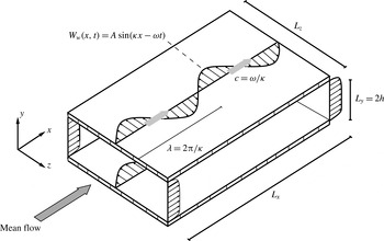
Schematic of a turbulent channel flow modified by streamwise-travelling waves of spanwise-wall velocity, with amplitude
 $A$
, streamwise wavenumber
 $\unicode[STIX]{x1D705}$
and angular frequency
 $\unicode[STIX]{x1D714}$
. Here
 $\unicode[STIX]{x1D706}$
is the streamwise wavelength;
 $c$
is the phase speed of the waves; and
 $L_{x}$
,
 $L_{y}=2h$
and
 $L_{z}$
are the dimensions of the computational domain in the streamwise, wall-normal and spanwise directions, respectively.

DNS of the turbulent flow in a doubly periodic channel are used to study the effect of the Reynolds number
 $Re$
on the reduction of turbulent drag achieved by streamwise-travelling waves of spanwise-wall velocity (Quadrio et al.
Reference Quadrio, Ricco and Viotti2009), imposed on both walls as the boundary condition:
 $$\begin{eqnarray}\displaystyle W_{w}(x,t)=A\sin (\unicode[STIX]{x1D705}x-\unicode[STIX]{x1D714}t). & & \displaystyle\end{eqnarray}$$
In the above expression for the wall forcing,
 $W_{w}$
is the spanwise velocity enforced at the wall,
 $A$
is the amplitude of the forcing,
 $\unicode[STIX]{x1D705}$
is the streamwise wavenumber,
 $\unicode[STIX]{x1D714}$
is the angular frequency, and
 $x$
and
 $t$
are the streamwise coordinate and time, respectively. The forcing, sketched in figure 1, consists of a wall distribution of streamwise-modulated waves of the spanwise (
 $z$
) velocity component with wavelength
 $\unicode[STIX]{x1D706}=2\unicode[STIX]{x03C0}/\unicode[STIX]{x1D705}$
and period
 $T=2\unicode[STIX]{x03C0}/\unicode[STIX]{x1D714}$
, which travel at speed
 $c=\unicode[STIX]{x1D714}/\unicode[STIX]{x1D705}$
forwards (
 $c>0$
) or backwards (
 $c<0$
) with respect to the direction
 $x$
of the mean flow. The three independent parameters (for example,
 $A$
,
 $\unicode[STIX]{x1D705}$
and
 $\unicode[STIX]{x1D714}$
) of the control law (2.1) combined with the Reynolds number
 $Re$
define a four-dimensional parameter space, whose complete investigation represents a computational challenge.
The simulations have been run with the solver for the incompressible Navier–Stokes equations developed by Luchini & Quadrio (Reference Luchini and Quadrio2006), and adapted in this work to run on a Blue Gene/Q system at the Italian Supercomputing Center CINECA, where most of the calculations were carried out. Simulations enforcing either a constant flow rate (CFR) or a constant pressure gradient (CPG) (for details, see Hasegawa, Quadrio & Frohnapfel Reference Hasegawa, Quadrio and Frohnapfel2014; Quadrio, Frohnapfel & Hasegawa Reference Quadrio, Frohnapfel and Hasegawa2016) are considered. The aim is to obtain and compare two comprehensive sets of cases at
 $Re_{\unicode[STIX]{x1D70F}}=200$
and
 $1000$
, where
 $Re_{\unicode[STIX]{x1D70F}}=u_{\unicode[STIX]{x1D70F}}h/\unicode[STIX]{x1D708}$
is the Reynolds number based on the channel half-height
 $h$
, the friction velocity
 $u_{\unicode[STIX]{x1D70F}}$
of the uncontrolled flow and the kinematic viscosity
 $\unicode[STIX]{x1D708}$
of the fluid. This is enforced directly in the CPG cases where the value of
 $Re_{\unicode[STIX]{x1D70F}}$
is specified as an input parameter, while in the CFR cases the imposed flow rate (hence the input value of
 $Re_{b}=U_{b}2h/\unicode[STIX]{x1D708}$
) leads to values of
 $Re_{\unicode[STIX]{x1D70F}}$
that only approximately correspond to the target. In the following, for ease of discussion, we will conventionally refer to the two case sets as the low-
 $Re$
(or
 $Re_{\unicode[STIX]{x1D70F}}=200$
) case set and the high-
 $Re$
(or
 $Re_{\unicode[STIX]{x1D70F}}=1000$
) case set.
In both case sets, the initial condition is that of an uncontrolled turbulent flow, and care is taken to begin the statistical analysis after properly discarding the initial transient (of duration up to 1000 viscous time units), where the control leads the flow towards a reduced level of friction drag. The spatial resolution in wall units is always better than
 $\unicode[STIX]{x0394}x^{+}=12.3$
and
 $\unicode[STIX]{x0394}z^{+}=6.1$
(or
 $\unicode[STIX]{x0394}x^{+}=8.2$
and
 $\unicode[STIX]{x0394}z^{+}=4.1$
if the additional modes used to completely remove the aliasing error are considered); and
 $\unicode[STIX]{x0394}y^{+}$
smoothly varies from
 $\unicode[STIX]{x0394}y^{+}\approx 1$
near the wall to
 $\unicode[STIX]{x0394}y^{+}\approx 7$
at the centreline. In the CFR cases, the spatial resolution in every direction strongly improves with drag reduction and the related drop in
 $Re_{\unicode[STIX]{x1D70F}}$
. Time integration is carried out with a partially implicit approach, with a Crank–Nicolson scheme for the viscous terms and a third-order Runge–Kutta scheme for the convective terms. The Courant–Friedrichs–Lewy (CFL) number is set at unity, well below the stability limit of the temporal integration scheme; the consequent average size of the time step is always below
 $\unicode[STIX]{x0394}t^{+}=0.17$
for the low-
 $Re$
cases, and below
 $\unicode[STIX]{x0394}t^{+}=0.1$
for the high-
 $Re$
cases. The duration of the simulation obviously affects the quality of the estimate of the mean value of drag: the total integration time is thus adjusted in order to reach an acceptably small uncertainty over the whole dataset. The integration time is at least 24 000 viscous time units, and in certain cases it increases up to 80 000 viscous units. For each value of
 $Re$
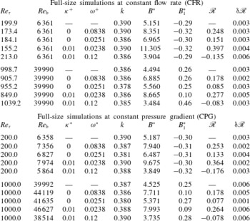
, the computational study considers two distinct sets of simulations, described below, details of which are reported in table 1.
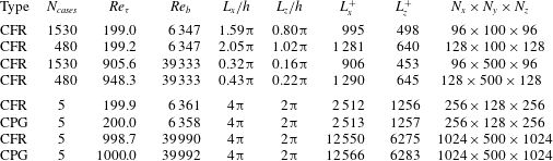
Details of the small-box (upper half) and large-box (lower half) simulations. Every case set is detailed in terms of simulation type (CFR or CPG), number of cases
 $N_{cases}$
, values of friction Reynolds number
 $Re_{\unicode[STIX]{x1D70F}}$
and bulk Reynolds number
 $Re_{b}$
, length and width of the computational domain in inner and outer units, number of Fourier modes in the homogeneous directions (additional modes are used for dealiasing, according to the
 $3/2$
rule) and collocation points in the wall-normal direction.

2.1 The small-box large database
The first set (upper half of table 1) is a parameter study designed to produce a massive database of drag-reduction data (4020 cases overall); the parameter space includes the forcing wavenumber
 $\unicode[STIX]{x1D705}$
, the forcing angular frequency
 $\unicode[STIX]{x1D714}$
and, for the first time, the forcing amplitude
 $A$
too. For each
 $Re$
, six values of
 $A^{+}=\{2,4.5,5.5,7,12,20\}$
, a wide frequency range
 $-0.5\leqslant \unicode[STIX]{x1D714}^{+}\leqslant 1$
and 13 different values of
 $\unicode[STIX]{x1D705}^{+}$
are considered, between the limiting case
 $\unicode[STIX]{x1D705}^{+}=0$
when the control law (2.1) reduces to the classic spanwise-oscillating wall and the maximum considered wavenumber
 $\unicode[STIX]{x1D705}^{+}=0.05$
. Previous knowledge of the drag-reduction pattern is exploited to focus on the interesting regions of the parameter space through a non-uniform distribution of the simulation points. Values of
 $A^{+}$
are chosen to describe reasonably well the region for maximum energy efficiency near
 $A^{+}=5$
, to include the point
 $A^{+}=12$
that corresponds to most available information (Quadrio et al.
Reference Quadrio, Ricco and Viotti2009; Touber & Leschziner Reference Touber and Leschziner2012; Hurst et al.
Reference Hurst, Yang and Chung2014), and to include an additional point at larger
 $A^{+}$
to better characterize the absolute maximum of drag reduction. Availability of data at different
 $A^{+}$
is essential for appreciating the difference, discussed below, between ‘reference
 $u_{\unicode[STIX]{x1D70F}}$
’ or
 $+$
scaling and ‘actual
 $u_{\unicode[STIX]{x1D70F}}$
’ or
 $\ast$
scaling.
For this set of calculations, carried out under the CFR condition, a relatively small computational domain (whose dimensions are kept constant in wall units when
 $Re$
is increased) is employed: the consequent savings in computing time are key to make this huge parameter study possible. For each value of
 $Re_{b}$
, adjusted to yield the target value of
 $Re_{\unicode[STIX]{x1D70F}}$
as nearly as practicable, two subsets of simulations are reported in table 1, which differ for the slightly different value of the length
 $L_{x}$
of the computational domain. Since the wavelength of the wall forcing is constrained to integer submultiples of the box length, this mitigates the quantization effect and allows a better investigation of the lower forcing wavenumbers. In changing box size, the aspect ratio of the computational domain is always kept constant at
 $L_{x}=2L_{z}$
, and the number of Fourier modes in the wall-parallel directions is adjusted to keep the spatial resolution in wall units unchanged.
2.2 The large-box small database
The second set of simulations (lower half of table 1) employs a larger domain size, whose dimensions are kept constant in outer units when
 $Re$
is increased. Owing to the larger computational cost, only a few representative cases are computed. For both
 $Re$
, we consider the reference uncontrolled case, and four other cases at the amplitude
 $A^{+}=7$
, which is a control amplitude near the largest net savings. One case is for the oscillating wall at nearly optimal period
 $T^{+}=75$
, one case with oscillating wall at the larger period
 $T^{+}=250$
, one case with travelling waves with large drag reduction (
 $\unicode[STIX]{x1D714}^{+}=0.0239$
and
 $\unicode[STIX]{x1D705}^{+}=0.01$
) and one case for travelling waves with drag increase (
 $\unicode[STIX]{x1D714}^{+}=0.12$
and
 $\unicode[STIX]{x1D705}^{+}=0.01$
). Each case is run under both CFR and CPG (and for the latter the forcing parameters listed above are to be intended in actual wall units), for a total of 20 simulations featuring the larger computational domain.
2.3 Domain size and uncertainty
For the simulations described in § 2.1, the computational domain is rather small, with a streamwise length of the order of 1000 wall units (one half of that for the domain width). Such domains, which imply a reduced computational cost per time step, have already been used in the past for similar studies. Although several times larger than the minimal domain shown by Jiménez & Moin (Reference Jiménez and Moin1991) to be capable of sustaining the near-wall turbulent cycle, the present computational domain is not large enough to guarantee flow statistics truly independent of spatial truncation. The large outer structures that become more and more important as
 $Re$
increases do not entirely fit into such a small domain, the mean velocity in the outer region progressively deviates from the correct profile, and even the prediction of wall friction is affected by an error. A trace of this can be observed in table 1, where at high
 $Re$
a 35 % increase in box length brings approximately a 5 % change in
 $Re_{\unicode[STIX]{x1D70F}}$
.
However, Gatti & Quadrio (Reference Gatti and Quadrio2013) demonstrated that reliable information concerning drag reduction can still be extracted from such simulations. In fact, most of the inaccuracy in predicting friction cancels out when the two friction coefficients (with and without control) are subtracted to compute drag reduction. It must be noted that the much shorter computing time per time step comes at the cost of a larger number of time steps required to obtain meaningful temporal averages of spatially averaged quantities, which present larger temporal fluctuations as a consequence of the lesser contribution of the spatial average (Jiménez & Moin Reference Jiménez and Moin1991). Lozano-Durán & Jiménez (Reference Lozano-Durán and Jiménez2014b ) have shown that the standard deviation of the spatially averaged skin friction is roughly inversely proportional to the square root of the area of the computational box. Hence, it is imperative to monitor the statistical uncertainty of the main quantities, and to increase the averaging time (i.e. the duration of the simulations) until the uncertainty reduces to an acceptable level.
In the present paper, the main quantity of interest is the drag-reduction rate
 $\mathscr{R}$
, as defined in (1.1). Its uncertainty
 $\unicode[STIX]{x03B4}\mathscr{R}$
is written by propagating the standard uncertainty of the skin-friction coefficients for the uncontrolled and controlled flows, and by assuming they are independent variables,
 $$\begin{eqnarray}\displaystyle \unicode[STIX]{x03B4}\mathscr{R}=\frac{C_{f}}{C_{f,0}}\sqrt{\left(\frac{\unicode[STIX]{x03B4}C_{f}}{C_{f}}\right)^{2}+\left(\frac{\unicode[STIX]{x03B4}C_{f,0}}{C_{f,0}}\right)^{2}}, & & \displaystyle\end{eqnarray}$$
and then extended to a 95 % confidence interval. The standard uncertainties
 $\unicode[STIX]{x03B4}C_{f,0}$
and
 $\unicode[STIX]{x03B4}C_{f}$
are evaluated with the procedure described by Oliver et al. (Reference Oliver, Malaya, Ulerich and Moser2014), by calculating an integral time scale via an autoregressive method. This is slightly different from the strategy employed by Gatti & Quadrio (Reference Gatti and Quadrio2013), who estimated the time scale differently, and it is interesting to note that the two methods end up with essentially the same result. For instance, when applied to the time history of skin friction in an unmanipulated channel flow at
 $Re_{\unicode[STIX]{x1D70F}}=200$
, with domain size
 $L_{x}=4\unicode[STIX]{x03C0}h,~L_{z}=2\unicode[STIX]{x03C0}h$
and an integration time of
 $4480h/U_{b}$
, the present method yields a relative standard uncertainty of 0.70 % while the method by Gatti & Quadrio (Reference Gatti and Quadrio2013) yields the slightly lower value of 0.66 %. Similar values of 0.61 % and 0.64 % are obtained respectively with the well-known method of non-overlapping batch means (Schmeiser Reference Schmeiser1982), which is related to the procedure followed by Hoyas & Jiménez (Reference Hoyas and Jiménez2008), and the similar method proposed by Mockett, Knacke & Thiele (Reference Mockett, Knacke and Thiele2010), which relies on the known statistical properties of white noise. The present method provides the most conservative estimate.
The uncertainty on the value of other quantities, such as the mean velocity profile or the control performance estimators presented below, is computed analogously. Hereinafter the uncertainty is always reported in the text when applicable and represented with error bars or shading in all the relevant figures.
3 Results
3.1 Validation for the oscillating wall
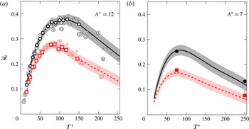
Drag-reduction rate
 $\mathscr{R}$
versus period of wall oscillation
 $T^{+}$
at
 $A^{+}=12$
in reference scaling (a) and versus
 $T^{\ast }$
at
 $A^{\ast }=7$
in actual scaling (b). Black (darker) colour identifies low-
 $Re$
data, and red (lighter) colour corresponds to high-
 $Re$
data. Present data are identified by large symbols connected with thick lines, with the shaded area representing the corresponding interval at 95 % confidence level. In panel (a), small open symbols are from Gatti & Quadrio (Reference Gatti and Quadrio2013), while symbols with letters identify literature data: Q, Quadrio & Ricco (Reference Quadrio and Ricco2004); T, Touber & Leschziner (Reference Touber and Leschziner2012); H, Hurst et al. (Reference Hurst, Yang and Chung2014) with the higher
 $Re$
data at
 $Re_{\unicode[STIX]{x1D70F}}=800$
. In panel (b), present data are represented by thick lines only, because these are obtained through linear interpolation, while symbols are present data for large-box simulations.

We show first the results for the temporal oscillation of the wall (i.e.
 $\unicode[STIX]{x1D705}=0$
), which can be used as a further validation of the present dataset, thanks to the availability of several literature data at various
 $Re$
. Figure 2(a) shows the drag-reduction rate against the period of wall oscillation
 $T^{+}$
for oscillations with an amplitude of
 $A^{+}=12$
in reference inner scaling. At
 $Re_{\unicode[STIX]{x1D70F}}=200$
the present results agree very well with those from Gatti & Quadrio (Reference Gatti and Quadrio2013), who employed a comparable domain size, as well as with the full-size simulations of Touber & Leschziner (Reference Touber and Leschziner2012) and Hurst et al. (Reference Hurst, Yang and Chung2014). An optimal oscillation period exists at
 $T^{+}=100{-}125$
(Baron & Quadrio Reference Baron and Quadrio1996; Yakeno, Hasegawa & Kasagi Reference Yakeno, Hasegawa and Kasagi2014), which maximizes at every
 $A^{+}$
the interaction of the oscillating Stokes layer of proper thickness with the convecting turbulence structures. At optimal values of
 $T^{+}$
and
 $A^{+}=12$
, for instance, values
 $\mathscr{R}=0.385$
(Touber & Leschziner Reference Touber and Leschziner2012)
 $\mathscr{R}=0.364$
(Hurst et al.
Reference Hurst, Yang and Chung2014) and
 $\mathscr{R}=0.384$
(Gatti & Quadrio Reference Gatti and Quadrio2013) have been observed. All agree well with the present value of
 $0.374\pm 0.018$
. The only exception is the data point at
 $T^{+}\approx 200$
by Hurst et al. (Reference Hurst, Yang and Chung2014), which lies well below the other datasets. (It is possible that their averaging time was chosen too small and/or not as an integer multiple of the oscillation period: at large
 $T^{+}$
the wall friction exhibits significant periodic oscillations. Indeed, travelling-wave data by Hurst et al. (Reference Hurst, Yang and Chung2014), which are not affected by this problem, agree very well with the present and other results: see figure 7 below.) The comparison against the reference dataset by Quadrio & Ricco (Reference Quadrio and Ricco2004) confirms the slight (less than 0.02) overestimation of
 $\mathscr{R}$
in a narrow region close to the optimal period
 $T^{+}\approx 100$
, already known (see the discussion of figures 5 and 6 in Gatti & Quadrio (Reference Gatti and Quadrio2013)) and attributed to domain-size effects; this is limited to the region of largest drag reduction (
 $\mathscr{R}>0.3$
) and becomes milder for streamwise-travelling waves (
 $\unicode[STIX]{x1D705}>0$
). The agreement between the present dataset and the available literature data is excellent also at
 $Re_{\unicode[STIX]{x1D70F}}=1000$
. The data points by Hurst et al. (Reference Hurst, Yang and Chung2014) lie slightly above the present results for small oscillation periods, but it must be recalled that they are computed at the lower
 $Re_{\unicode[STIX]{x1D70F}}=800$
. As already known (Gatti & Quadrio Reference Gatti and Quadrio2013; Hurst et al.
Reference Hurst, Yang and Chung2014), the optimal oscillation period decreases with
 $Re$
and becomes
 $T^{+}\approx 75$
at
 $Re_{\unicode[STIX]{x1D70F}}=1000$
. At this value of
 $T^{+}$
a drag reduction of
 $0.277\pm 0.016$
is measured, which is very close to
 $\mathscr{R}=0.275$
measured by Hurst et al. (Reference Hurst, Yang and Chung2014) and
 $\mathscr{R}=0.29$
reported by Touber & Leschziner (Reference Touber and Leschziner2012) at
 $T^{+}=100$
.
Figure 2(b) shows
 $\mathscr{R}$
versus
 $T^{\ast }$
at constant
 $A^{\ast }=7$
, i.e. with actual viscous scaling, which would require data from simulations driven at CPG. The present small-box simulations are indeed computed at CFR, but the availability of data at several values of
 $A^{+}$
makes a
 $\ast$
scaling possible through interpolation. As far as we know, no such data exist for
 $Re_{\unicode[STIX]{x1D70F}}=1000$
or nearby; the only data we can compare with are the large-domain CPG simulations described in table 1, and this motivates the choice of the amplitude
 $A^{\ast }=7$
. At
 $Re_{\unicode[STIX]{x1D70F}}=200$
the optimal period is
 $T^{\ast }\approx 75$
, where a drag reduction of
 $0.255\pm 0.020$
is achieved. This value is very close to
 $0.253\pm 0.002$
of the large-domain data point at the same
 $T^{\ast }$
. Good agreement between the present full-size DNS and reduced-domain database is evident also at
 $Re_{\unicode[STIX]{x1D70F}}=1000$
, where at
 $T^{\ast }=75$
the former achieved
 $0.167\pm 0.015$
and the latter
 $0.175\pm 0.005$
. The shift of the optimal
 $T^{\ast }$
with
 $Re$
is, if present at all, much milder than that of
 $T^{+}$
, suggesting that actual inner scaling might be more appropriate. A possible rationale to explain the existence of the optimal oscillation period can be found in Yakeno et al. (Reference Yakeno, Hasegawa and Kasagi2014).
3.2 The whole dataset at a glance
Travelling-wave results are now presented as in Quadrio et al. (Reference Quadrio, Ricco and Viotti2009) and Hurst et al. (Reference Hurst, Yang and Chung2014), by plotting drag-reduction maps in the space of the control parameters
 $(\unicode[STIX]{x1D705}^{+},\unicode[STIX]{x1D714}^{+})$
at
 $A^{+}=12$
. The data just discussed in figure 2 are those lying on the
 $\unicode[STIX]{x1D705}=0$
horizontal axis. Note that, to produce such maps, first the raw results are interpolated on a finer Cartesian grid, without any smoothing or removal of outliers, and then contour lines are drawn on the Cartesian grid. Using
 $\ast$
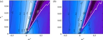
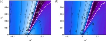
scaling also implies interpolation along the third axis (forcing amplitude). Figure 3 compares the drag-reduction rate
 $\mathscr{R}$
at
 $Re_{\unicode[STIX]{x1D70F}}=200$
and
 $1000$
. The map at
 $Re_{\unicode[STIX]{x1D70F}}=200$
reproduces the well-known shape described by Quadrio et al. (Reference Quadrio, Ricco and Viotti2009), with a maximum
 $\mathscr{R}$
at given
 $A^{+}=12$
of
 $\mathscr{R}_{m,A^{+}}=0.500\pm 0.015$
located at
 $(\unicode[STIX]{x1D714}^{+},\unicode[STIX]{x1D705}^{+})=(0.0195,0.0063)$
, which agrees with
 $\mathscr{R}_{m,A^{+}}=0.48$
at
 $(0.018,0.005)$
measured by Quadrio et al. (Reference Quadrio, Ricco and Viotti2009) and
 $\mathscr{R}_{m,A^{+}}=0.5$
at
 $(0.025,0.008)$
obtained by Hurst et al. (Reference Hurst, Yang and Chung2014). The triangular drag-increasing region associated (Quadrio et al.
Reference Quadrio, Ricco and Viotti2009) to a lock-in phenomenon between the travelling waves and the convecting turbulence structures is clearly evident and well captured. The side-by-side comparison with data at
 $Re_{\unicode[STIX]{x1D70F}}=1000$
clearly shows that, consistent with all previous information, the forcing becomes less effective as
 $Re$
grows, since both the largest drag reduction and drag increase weaken. The
 $\mathscr{R}_{m,A^{+}}$
value decreases to
 $0.388\pm 0.014$
and its location in the plane moves along the drag-reduction ridge towards higher frequencies and wavenumbers to
 $(\unicode[STIX]{x1D714}^{+},\unicode[STIX]{x1D705}^{+})=(0.05,0.0195)$
. It must be observed, however, that the precise location of
 $\mathscr{R}_{m,A^{+}}$
in the
 $(\unicode[STIX]{x1D714}^{+},\unicode[STIX]{x1D705}^{+})$
plane is not robust information, since the region of maximum drag reduction presents a rather flat peak. This is particularly true at
 $Re_{\unicode[STIX]{x1D70F}}=1000$
, where the contour level drawn for
 $\mathscr{R}=0.388-0.014$
, i.e.
 $\mathscr{R}_{m,A^{+}}$
minus its uncertainty, is an elongated region that almost encloses the low-
 $Re$
maximum. However, the decrease of
 $\mathscr{R}_{m,A^{+}}$
at larger
 $Re$
as well as its shift towards higher frequencies and wavenumbers is clear, and it agrees with previous evidence by Gatti & Quadrio (Reference Gatti and Quadrio2013) and by Hurst et al. (Reference Hurst, Yang and Chung2014), with the latter being based on fewer data at
 $Re_{\unicode[STIX]{x1D70F}}=800$
but computed on a larger computational domain.
Map of drag reduction
 $\mathscr{R}_{A^{+}}$
at constant forcing amplitude for streamwise-travelling waves at
 $A^{+}=12$
, for
 $Re_{\unicode[STIX]{x1D70F}}=200$
(a) and
 $Re_{\unicode[STIX]{x1D70F}}=1000$
(b). Contours are spaced by 0.1, negative contours are dashed. The thick white line corresponds to zero drag change, while the dash-dotted line is the locus of points where
 $\mathscr{R}=\mathscr{R}_{m,A^{+}}-\unicode[STIX]{x03B4}\mathscr{R}$
, and the cross indicates the position of
 $\mathscr{R}_{m,A^{+}}$
.

Isosurfaces of drag reduction
 $\mathscr{R}$
in the three-dimensional parameter space
 $(\unicode[STIX]{x1D714}^{+},\unicode[STIX]{x1D705}^{+},A^{+})$
for
 $Re_{\unicode[STIX]{x1D70F}}=200$
(a) and
 $Re_{\unicode[STIX]{x1D70F}}=1000$
(b). Isosurfaces from dark to light range from
 $\mathscr{R}=-0.2$
to 0.5 in steps of 0.1. The cloud of dots represents the 2010 data points where, at each
 $Re$
, a DNS has been carried out.

Map of drag reduction
 $\mathscr{R}_{A^{\ast }}$
at constant forcing amplitude for streamwise-travelling waves at
 $A^{\ast }=12$
, for
 $Re_{\unicode[STIX]{x1D70F}}=200$
(a) and
 $Re_{\unicode[STIX]{x1D70F}}=1000$
(b). Lines and symbols as in figure 3.

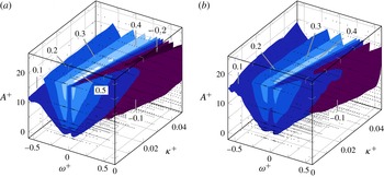
The present database contains much more information than that shown in figure 3, because several values of forcing amplitude are considered. Figure 4 shows the entire dataset at a glance in the three-dimensional parameter space
 $(\unicode[STIX]{x1D714}^{+},\unicode[STIX]{x1D705}^{+},A^{+})$
, in comparative form between the two Reynolds numbers. The three-dimensional field of
 $\mathscr{R}$
is visualized via isosurfaces of
 $\mathscr{R}=\text{const.}$
, and the cloud of tiny dots in the figure indicates the 4020 points where a DNS has been performed. Such an extensive database makes the description of
 $\mathscr{R}$
with actual inner scaling possible. In the past, only a few channel flow studies (e.g. Ricco et al.
Reference Ricco, Ottonelli, Hasegawa and Quadrio2012) have been performed at CPG, thus ensuring that drag reduction does not lead to changes in
 $Re_{\unicode[STIX]{x1D70F}}$
. When CFR is employed, a significant drop in the friction velocity and
 $Re_{\unicode[STIX]{x1D70F}}$
due to drag reduction implies that viscous units change, and in particular that the forcing for a given
 $A^{+}$
becomes stronger in physical units than the forcing for the same given value of
 $A^{\ast }$
. Using
 $+$
scaling is thus equivalent to employing outer scaling. Hence, the choice between
 $+$
and
 $\ast$
scaling leads to different scenarios (Quadrio Reference Quadrio2011). Since in the drag-reduced state only the actual viscous units are relevant,
 $\ast$
scaling should be adopted when comparing results obtained at different
 $Re$
. The present data have been computed on
 $A^{+}=\text{const.}$
planes, but they can be easily interpolated to produce figure 5, where a map of
 $\mathscr{R}$
in the
 $(\unicode[STIX]{x1D714}^{\ast },\unicode[STIX]{x1D705}^{\ast })$
plane at
 $A^{\ast }=12$
is shown. At
 $Re_{\unicode[STIX]{x1D70F}}=200$
, the maximum drag reduction at constant
 $A^{\ast }$
is
 $\mathscr{R}_{m,A^{\ast }}=0.453\pm 0.015$
at
 $(\unicode[STIX]{x1D714}^{\ast },\unicode[STIX]{x1D705}^{\ast })=(0.0167,0.067)$
, to be compared with
 $\mathscr{R}_{m,A^{+}}=0.500\pm 0.015$
at
 $(\unicode[STIX]{x1D714}^{+},\unicode[STIX]{x1D705}^{+})=(0.0195,0.0063)$
. This agrees with data at the same
 $A^{\ast }$
and
 $Re$
by Quadrio & Ricco (Reference Quadrio and Ricco2011), who drove the channel at CPG and found
 $\mathscr{R}_{m,A^{\ast }}=0.45$
at
 $(\unicode[STIX]{x1D714}^{\ast },\unicode[STIX]{x1D705}^{\ast })=(0.012,0.045)$
. At the higher
 $Re_{\unicode[STIX]{x1D70F}}=1000$
,
 $\mathscr{R}_{m,A^{\ast }}=0.343\pm 0.019$
at
 $(\unicode[STIX]{x1D714}^{\ast },\unicode[STIX]{x1D705}^{\ast })=(0.0246,0.0789)$
is observed instead of
 $\mathscr{R}_{m,A^{+}}=0.388\pm 0.014$
at
 $(\unicode[STIX]{x1D714}^{+},\unicode[STIX]{x1D705}^{+})=(0.05,0.0195)$
.
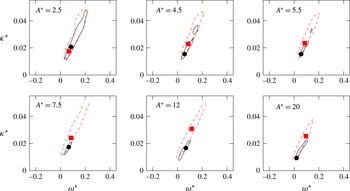
Region of large drag reduction, defined as the region where
 $\mathscr{R}$
is at least
 $\mathscr{R}_{m,A^{\ast }}-0.015$
, for various values of
 $A^{\ast }$
. Solid black lines,
 $Re_{\unicode[STIX]{x1D70F}}=200$
; dashed red lines,
 $Re_{\unicode[STIX]{x1D70F}}=1000$
. The location of
 $\mathscr{R}_{m,A^{\ast }}$
is marked by a black circle at
 $Re_{\unicode[STIX]{x1D70F}}=200$
and a red square at
 $Re_{\unicode[STIX]{x1D70F}}=1000$
.

Looking at
 $\mathscr{R}$
with different scalings leads to important remarks. First, the difference between
 $\mathscr{R}_{m,A^{+}}$
and
 $\mathscr{R}_{m,A^{\ast }}$
is small at
 $A^{+}=12$
. This is explained by the known weak dependence of
 $\mathscr{R}$
on
 $A$
at large amplitudes where saturation occurs (Quadrio et al.
Reference Quadrio, Ricco and Viotti2009). Indeed, at lower forcing intensities we observe a stronger drop, which at the lower
 $Re$
is from
 $\mathscr{R}_{m,A^{+}}=0.035\pm 0.016$
for
 $A^{+}=4.5$
to
 $\mathscr{R}_{m,A^{\ast }}=0.29\pm 0.015$
for
 $A^{\ast }=4.5$
. Second, the effect of
 $Re$
on the value of
 $\mathscr{R}_{m,A^{\ast }}$
is qualitatively similar to that on
 $\mathscr{R}_{m,A^{+}}$
, and the shift of the location of the maximum in the
 $(\unicode[STIX]{x1D714},\unicode[STIX]{x1D705})$
plane is confirmed. Since the maximum of drag reduction is rather flat, this last observation is better highlighted in figure 6 by observing, at several values of
 $A^{\ast }$
, how the shape and size of the region where
 $\mathscr{R}$
is nearly maximum change while
 $Re$
increases. This region is identified by the contour line drawn for
 $\mathscr{R}=\mathscr{R}_{m,A^{\ast }}-0.015$
, with 0.015 being a representative value of
 $\unicode[STIX]{x03B4}\mathscr{R}$
. For every value of
 $A^{\ast }$
, this region at
 $Re_{\unicode[STIX]{x1D70F}}=1000$
is found to be larger than that at
 $Re_{\unicode[STIX]{x1D70F}}=200$
, which is enclosed by the former but for a small part at low wavenumbers and frequencies.
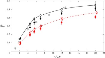
Maximum drag reduction
 $\mathscr{R}_{m,A}$
as a function of the forcing amplitude. Black continuous line and symbols are for low-
 $Re$
data, and red dashed line and symbols are for high-
 $Re$
data. At each
 $Re$
, open symbols refer to reference scaling (
 $\mathscr{R}_{m,A^{+}}$
against
 $A^{+}$
) and closed symbols to actual scaling (
 $\mathscr{R}_{m,A^{\ast }}$
against
 $A^{\ast }$
). As in figure 2, open symbols with letters are literature data. Note that Quadrio et al. (Reference Quadrio, Ricco and Viotti2009) assumed reference inner scaling for the optimal
 $(\unicode[STIX]{x1D714}^{+},\unicode[STIX]{x1D705}^{+})$
pair determined at
 $A^{+}=12$
.

A global view of the drag-reduction performance of the travelling waves as determined by the present dataset can be obtained from figure 7, which shows for both values of
 $Re$
how the maximum drag reduction
 $\mathscr{R}_{m,A}$
increases with the forcing amplitude. It is confirmed that, regardless of the scaling adopted, the general shape of the curve is always that of a saturated growth of
 $\mathscr{R}$
with
 $A$
, as already observed, for instance, for spanwise-wall oscillations by Quadrio & Ricco (Reference Quadrio and Ricco2004) and for streamwise-travelling waves by Quadrio et al. (Reference Quadrio, Ricco and Viotti2009). The curves with
 $\ast$
scaling are consistently lower than the curves with
 $+$
scaling, and data at
 $Re_{\unicode[STIX]{x1D70F}}=1000$
are lower than data at
 $Re_{\unicode[STIX]{x1D70F}}=200$
. Figure 7 also includes a few data points from Quadrio et al. (Reference Quadrio, Ricco and Viotti2009) at
 $Re_{\unicode[STIX]{x1D70F}}=200$
. Their point at
 $A^{+}=12$
falls slightly below the present data, something that Gatti & Quadrio (Reference Gatti and Quadrio2013) already documented as an effect of the limited computational domain. However, the larger values of
 $\mathscr{R}_{m,A^{+}}$
observed for
 $A^{+}<12$
in the present study also result from a better scan of the parameter space. In fact, Quadrio et al. (Reference Quadrio, Ricco and Viotti2009) simply assumed a simple (reference) viscous scaling for the location of
 $\mathscr{R}_{m,A^{+}}$
, whereas here a full parameter study avoids this assumption and determines that
 $\mathscr{R}_{m,A^{+}}=0.38\pm 0.017$
can still be achieved at
 $A^{+}=5.5$
and
 $Re_{\unicode[STIX]{x1D70F}}=200$
, which becomes
 $\mathscr{R}_{m,A^{+}}=0.26\pm 0.020$
at
 $Re_{\unicode[STIX]{x1D70F}}=1000$
. The comparison at
 $A^{+}=12$
with the data from Hurst et al. (Reference Hurst, Yang and Chung2014) shows excellent agreement, considering that the slightly higher
 $\mathscr{R}$
of the high-
 $Re$
data point is due to its lower value of
 $Re_{\unicode[STIX]{x1D70F}}=800$
.
3.3 Performance indicators
Active techniques for skin-friction drag reduction should not be characterized by
 $\mathscr{R}$
alone: the net power saving rate
 $\mathscr{S}$
, which also accounts for the energy cost of the control, is an important additional figure of merit for a complete assessment. The rate
 $\mathscr{S}$
can be defined as
 $$\begin{eqnarray}\displaystyle \mathscr{S}=\mathscr{R}-\frac{P_{in}}{P_{0}}, & & \displaystyle\end{eqnarray}$$
where
 $P_{0}$
is the power (per unit area) required to drive the uncontrolled channel flow, and
 $P_{in}$
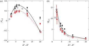
is the control input power, computed here following Baron & Quadrio (Reference Baron and Quadrio1996) by neglecting the mechanical losses of a real actuator. Figure 8(a) presents the maximum net power saving
 $\mathscr{S}_{m,A}$
at given amplitude. At both
 $Re$
the largest
 $\mathscr{S}_{m,A}$
is observed at
 $A^{+}\approx 6$
, where the travelling waves yield
 $\mathscr{S}_{m,A^{+}}=0.31\pm 0.021$
at
 $Re_{\unicode[STIX]{x1D70F}}=200$
and
 $\mathscr{S}_{m,A^{+}}=0.19\pm 0.018$
at
 $Re_{\unicode[STIX]{x1D70F}}=1000$
. In comparison with existing data from Quadrio et al. (Reference Quadrio, Ricco and Viotti2009), there is a noticeable improvement due to the more detailed scan of the parameter space at low forcing amplitude. As observed by Ricco & Quadrio (Reference Ricco and Quadrio2008) and Gatti & Quadrio (Reference Gatti and Quadrio2013), the power expenditure per unit pumping power
 $P_{in}/P_{0}$
decreases with
 $Re$
at a rate proportional to
 $Re_{\unicode[STIX]{x1D70F}}^{-0.136}$
and faster than
 $\mathscr{R}$
in many parts of the control parameter space. This means that
 $\mathscr{S}$
decreases as
 $\mathscr{R}$
, or at a slower rate. Also,
 $\mathscr{S}_{m,A^{\ast }}$
is slightly lower than
 $\mathscr{S}_{m,A^{+}}$
at both
 $Re$
up to
 $A^{\ast }\approx 7$
. In this range of forcing amplitudes, the main contributor to
 $\mathscr{S}$
is
 $\mathscr{R}$
, the input power being much smaller, and
 $\mathscr{R}$
obtained for a given
 $A^{\ast }$
is lower than
 $\mathscr{R}$
obtained for a given
 $A^{+}$
. Starting from
 $A^{\ast }\approx 7$
, the opposite occurs, and
 $\mathscr{S}_{m,A^{\ast }}$
becomes larger than
 $\mathscr{S}_{m,A^{+}}$
, because at high forcing amplitude
 $\mathscr{S}$
is dominated by
 $-P_{in}/P_{0}$
, which is smaller (in absolute value) when forcing is considered at given
 $A^{\ast }$
than at
 $A^{+}$
.
Maximum net power saving
 $\mathscr{S}_{m,A}$
(a) and maximum control gain
 $\mathscr{G}_{m,A}$
(b) as functions of the forcing amplitude. Lines and symbols are as in figure 7.

The control gain
 $\mathscr{G}$
is defined as the power benefit per unit control power,
 $$\begin{eqnarray}\displaystyle \mathscr{G}=\frac{\mathscr{R}P_{0}}{P_{in}}, & & \displaystyle\end{eqnarray}$$
and is plotted in figure 8(b). Gain
 $\mathscr{G}_{m,A^{+}}$
increases rapidly for decreasing forcing amplitude, since
 $P_{in}$
is proportional to the square root of
 $A$
(Quadrio & Ricco Reference Quadrio and Ricco2011), while
 $\mathscr{R}$
varies less than linearly with
 $A$
. At the amplitude value yielding the largest
 $\mathscr{S}_{m,A^{+}}$
, we measure
 $\mathscr{G}=5.3\pm 0.24$
at
 $Re_{\unicode[STIX]{x1D70F}}=200$
and
 $\mathscr{G}=3.9\pm 0.31$
at
 $Re_{\unicode[STIX]{x1D70F}}=1000$
, with a mild decrease with
 $Re$
. In fact, the beneficial
 $Re$
effect on
 $P_{in}/P_{0}$
is even more effective on
 $\mathscr{G}$
than on
 $\mathscr{S}$
.
4 The effect of
 $Re$
on drag reduction

We now focus our attention on understanding how the drag-reduction performance of the streamwise-travelling waves is affected by an increase of the Reynolds number.
4.1 Characterizing
$\mathscr{R}$
via a power law

Power-law exponent
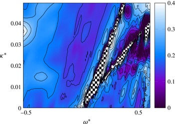
 $\unicode[STIX]{x1D6FE}$
as a function of
 $\unicode[STIX]{x1D705}^{\ast }$
and
 $\unicode[STIX]{x1D714}^{\ast }$
at
 $A^{\ast }=12$
, measured according to the formula (4.2). Contour lines are from 0 to 0.45 in 10 steps. In the regions marked by the chequerboard pattern, the exponent
 $\unicode[STIX]{x1D6FE}$
is undefined.

The effect of
 $Re$
on
 $\mathscr{R}$
has been traditionally quantified, as discussed in § 1, by assuming (Choi et al.
Reference Choi, Xu and Sung2002; Duque-Daza et al.
Reference Duque-Daza, Baig, Lockerby, Chernyshenko and Davies2012; Moarref & Jovanović Reference Moarref and Jovanović2012; Touber & Leschziner Reference Touber and Leschziner2012; Belan & Quadrio Reference Belan and Quadrio2013) that
 $\mathscr{R}$
decreases with
 $Re$
according to a simple power law, i.e.
 $$\begin{eqnarray}\displaystyle \mathscr{R}\propto Re_{\unicode[STIX]{x1D70F}}^{-\unicode[STIX]{x1D6FE}}. & & \displaystyle\end{eqnarray}$$
The power-law assumption was originally adopted by Choi et al. (Reference Choi, Xu and Sung2002) to fit early DNS-computed drag-reduction results obtained for the spanwise-oscillating wall, and it is not endowed with a specific physical significance. Recently, Gatti & Quadrio (Reference Gatti and Quadrio2013) and Hurst et al. (Reference Hurst, Yang and Chung2014) observed that
 $\unicode[STIX]{x1D6FE}$
is not a simple constant, but depends on the control parameters
 $\unicode[STIX]{x1D714}$
,
 $\unicode[STIX]{x1D705}$
and
 $A$
. The function
 $\unicode[STIX]{x1D6FE}=\unicode[STIX]{x1D6FE}(\unicode[STIX]{x1D714}^{\ast },\unicode[STIX]{x1D705}^{\ast },A^{\ast })$
can easily be constructed from the present dataset. For a given
 $(\unicode[STIX]{x1D714}^{\ast },\unicode[STIX]{x1D705}^{\ast },A^{\ast })$
combination, one knows the drag-reduction values
 $\mathscr{R}_{200}$
and
 $\mathscr{R}_{1000}$
measured at
 $Re_{\unicode[STIX]{x1D70F}}=200$
and
 $1000$
, and
 $\unicode[STIX]{x1D6FE}$
can be computed as
 $$\begin{eqnarray}\displaystyle \unicode[STIX]{x1D6FE}=\frac{\ln (\mathscr{R}_{200}/\mathscr{R}_{1000})}{\ln (200/1000)}. & & \displaystyle\end{eqnarray}$$
This quantity is shown in figure 9 for
 $A^{\ast }=12$
. The details might certainly change, depending, for example, on the specific value of
 $A^{\ast }$
, on the choice between working at constant
 $A^{+}$
or constant
 $A^{\ast }$
, or on the choice between using in (4.2) the nominal values of
 $Re_{\unicode[STIX]{x1D70F}}$
or the actual ones reported in table 1. However, the picture that emerges is consistently as rich as it is chaotic. The known result that
 $\unicode[STIX]{x1D6FE}$
varies strongly across the parameter space is easily confirmed, and this implies that some regions are more sensitive than others to the increase in
 $Re$
. For example, in most of the ridge of large drag reduction,
 $\unicode[STIX]{x1D6FE}$
assumes intermediate values between 0.1 and 0.15, while the largest values are seen in the low-wavenumber region of the drag-increase valley.
The complexity of figure 9 graphically illustrates how
 $\unicode[STIX]{x1D6FE}$
is not well suited to comprehensively describe the effect of
 $Re$
on the drag reduction. Indeed,
 $\unicode[STIX]{x1D6FE}$
is an ill-conditioned quantity, which is sensitive to small uncertainties in
 $\mathscr{R}$
, and according to definition (4.2) it grows to infinity whenever either
 $\mathscr{R}_{200}$
or
 $\mathscr{R}_{1000}$
is zero, while it becomes undefined when drag reduction at one
 $Re$
turns into drag increase at the other
 $Re$
(see the chequerboard-marked areas in figure 9). However, the most significant conceptual drawback of using
 $\unicode[STIX]{x1D6FE}$
is that, owing to the lack of physical rationale in the assumption of a power-law behaviour, extrapolation of existing data at higher
 $Re$
(for example, those which are typical of aeronautical applications) is entirely arbitrary. In fact,
 $\unicode[STIX]{x1D6FE}$
might well be a function of
 $Re$
too, as some results by Hurst et al. (Reference Hurst, Yang and Chung2014) seem to indicate. Hence, in our view,
 $\unicode[STIX]{x1D6FE}$
should be merely regarded as a (not well-conditioned) indicator with the same limited predictive capability of other, more trivial quantities, like the relative decrease of drag reduction. In the following, we will overcome the problem by introducing a more physically sound indicator.
4.2 Characterizing
$\mathscr{R}$
via the vertical shift
$\unicode[STIX]{x0394}B$
of the mean velocity profile


When dealing with distributed wall roughness (also including those particular roughness distributions, like streamwise-aligned riblets, that reduce friction drag instead of increasing it), it is well known that the consequent friction changes are reflected in the logarithmic region of the velocity profile. According to the classical theory (Pope Reference Pope2000), the streamwise mean velocity profile
 $\langle u\rangle (y)$
over a smooth wall (for which the distinction between the reference inner scaling
 $+$
and the actual inner scaling
 $\ast$
is irrelevant) presents a thin near-wall region, called the viscous sublayer, where
 $\langle u\rangle ^{+}=y^{+}$
, which is connected through the buffer region to the logarithmic layer, where the profile follows a logarithmic law:
 $$\begin{eqnarray}\displaystyle \langle u\rangle ^{+}=\frac{1}{k}\ln y^{+}+B. & & \displaystyle\end{eqnarray}$$
In the above expression,
 $k$
is the von Kármán constant and
 $B$
is the so-called additive constant or near-wall intercept. Both constants are known to assume values that depend weakly on
 $Re$
when
 $Re$
is low. For instance, Kim, Moin & Moser (Reference Kim, Moin and Moser1987) reported
 $k=0.4$
and
 $B=5.5$
at
 $Re_{\unicode[STIX]{x1D70F}}=180$
, whereas
 $k=0.386$
and
 $B=4.40$
at
 $Re_{\unicode[STIX]{x1D70F}}=4079$
or
 $k=0.384$
and
 $B=4.27$
at
 $Re_{\unicode[STIX]{x1D70F}}=5200$
have been reported, respectively, by Bernardini, Pirozzoli & Orlandi (Reference Bernardini, Pirozzoli and Orlandi2014) and Lee & Moser (Reference Lee and Moser2015). As stressed by Jiménez (Reference Jiménez2004), the additive constant
 $B$
is determined by the no-slip boundary condition at the wall, but, since the logarithmic law is only valid for
 $y^{+}\gg 1$
, its value depends on the details of the buffer and viscous layers. In the region further from the wall, the velocity-defect law, which describes the difference between the local mean velocity and the centreline mean velocity
 $U_{c}$
, takes the following form (Pope Reference Pope2000):
 $$\begin{eqnarray}\displaystyle U_{c}^{+}-\langle u\rangle ^{+}=-\frac{1}{k}\ln \left(\frac{y}{h}\right)+B_{1}, & & \displaystyle\end{eqnarray}$$
where
 $B_{1}$
is a flow-dependent constant representing the difference between the actual centreline velocity
 $U_{c}$
and the velocity value obtained by extrapolating the velocity-defect law up to the centreline. In channel flows,
 $B_{1}$
is close to zero (Pope Reference Pope2000).
If the logarithmic law (4.3) and the defect law (4.4) are added together, and
 $U_{c}$
is substituted with the more convenient
 $U_{b}$
thanks to the relation
 $U_{c}^{+}=U_{b}^{+}+1/\unicode[STIX]{x1D705}$
(Pope Reference Pope2000), the use of the definition (1.2) for the friction coefficient
 $C_{f}$
leads to the following friction law, i.e. an implicit relationship between
 $C_{f}$
and the Reynolds number
 $Re_{\unicode[STIX]{x1D70F}}$
,
 $$\begin{eqnarray}\displaystyle \sqrt{\frac{2}{C_{f}}}=\frac{1}{k}\ln Re_{\unicode[STIX]{x1D70F}}+B+B_{1}-\frac{1}{k}. & & \displaystyle\end{eqnarray}$$
When surface roughness is present, a classical statistical description of its effects (see e.g. Clauser Reference Clauser1956; Jiménez Reference Jiménez2004) is via the so-called roughness function, which quantifies the roughness-induced drag change via the downward shift of the velocity profile in the logarithmic layer, i.e. via the (negative) change
 $\unicode[STIX]{x0394}B$
of the additive constant
 $B$
. The same approach is used for the drag-reducing riblets (Luchini, Manzo & Pozzi Reference Luchini, Manzo and Pozzi1991; García-Mayoral & Jiménez Reference García-Mayoral and Jiménez2011), which produce a positive
 $\unicode[STIX]{x0394}B$
. Luchini (Reference Luchini, Desideri, Hirsch and Tallec1996) has shown that
 $\unicode[STIX]{x0394}B$
is equivalent to the amount of drag reduction, and is proportional to the so-called protrusion height, defined as the distance between two virtual wall-parallel planes where no-slip boundary conditions for the profiles of the spanwise and streamwise velocity components hold.
One is naturally led to think that what applies to changes in wall geometry (roughness) might apply as well to the present wall-based control strategy. Hence, our initial step consists in verifying whether the travelling waves consistently produce a vertical shift
 $\unicode[STIX]{x0394}B$
of the mean velocity profile. This is a known result (see e.g. Baron & Quadrio Reference Baron and Quadrio1996; Choi, DeBisschop & Clayton Reference Choi, DeBisschop and Clayton1998; Ricco & Wu Reference Ricco and Wu2004; Yudhistira & Skote Reference Yudhistira and Skote2011; Ricco et al.
Reference Ricco, Ottonelli, Hasegawa and Quadrio2012; Touber & Leschziner Reference Touber and Leschziner2012; Hurst et al.
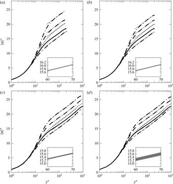
Reference Hurst, Yang and Chung2014; Skote Reference Skote2014) that is systematically checked in figure 10(a–d). The mean velocity profiles are obtained at both
 $Re$
from the large-box simulations described in § 2.2 (discretization details have been reported in the lower half of table 1). Since we do not want to limit the discussion to the case of maximum drag reduction, at each
 $Re$
five different cases are computed: the no-control case (solid line) and four additional ones, all with forcing amplitude of
 $A^{+}=7$
. These are two oscillating wall cases at
 $T^{+}=75$
and
 $T^{+}=250$
, and two travelling-wave cases, one with drag reduction at
 $\unicode[STIX]{x1D714}^{+}=0.0238$
and
 $\unicode[STIX]{x1D705}^{+}=0.01$
, and one with drag increase at
 $\unicode[STIX]{x1D714}^{+}=0.12$
and
 $\unicode[STIX]{x1D705}^{+}=0.01$
. Every case is computed twice, at the nominal value of
 $Re_{b}$
with CFR and at the nominal value of
 $Re_{\unicode[STIX]{x1D70F}}$
with CPG. For the CPG cases, the viscous quantities mentioned above to define the control conditions must be intended in actual viscous units.
Mean velocity profiles obtained from the large-domain simulations reported in the lower half of table 1: (a,b)
 $Re_{\unicode[STIX]{x1D70F}}=200$
; (c,d)
 $Re_{\unicode[STIX]{x1D70F}}=1000$
; (a,c) CFR cases; (b,d) CPG cases. The solid line is the reference case and the other lines correspond to control yielding both drag reduction and drag increase (see text). The insets enlarge a portion of the logarithmic layer to show the (very small) statistical uncertainty at 95 % confidence, denoted by the shaded area.

Figure 10(a–d) confirms that the spanwise forcing consistently produces a rigid upward (when drag is reduced) or downward (when drag is increased) shift of the mean velocity profile in the logarithmic region, while the parameter
 $B_{1}$
and the von Kármán constant do not change appreciably. In other words, the effect of the spanwise forcing can be quantified via the change
 $\unicode[STIX]{x0394}B$
of the additive constant, regardless of the control type, the value of
 $Re$
and the simulation strategy. Similar observations were recently put forward by Skote (Reference Skote2014), who observed changes of
 $\unicode[STIX]{x0394}B$
with drag reduction obtained by spanwise oscillations in a turbulent boundary layer, as well as changes in the von Kármán constant. The changes in
 $k$
, however, are a direct consequence of the spatial transient present in the boundary layer setting, while in the present parallel flow
 $\unicode[STIX]{x0394}B$
fully describes the effect of the spanwise forcing.
Once the control is seen to modify the mean velocity profile through
 $\unicode[STIX]{x0394}B$
, we can follow what has already been done for riblets (by e.g. Luchini et al.
Reference Luchini, Manzo and Pozzi1991; García-Mayoral & Jiménez Reference García-Mayoral and Jiménez2011), and exploit the friction law (4.5) to obtain a dimensionless relation between the Reynolds number
 $Re_{\unicode[STIX]{x1D70F}}$
, the drag-reduction rate
 $\mathscr{R}$
and the control-induced change
 $\unicode[STIX]{x0394}B$
of the additive constant. Equation (4.5) can be written twice, once for the uncontrolled flow (characterized by
 $Re_{\unicode[STIX]{x1D70F},0}$
and
 $C_{f,0}$
) and once for the controlled flow (with
 $Re_{\unicode[STIX]{x1D70F}}$
and
 $C_{f}$
). By subtracting the latter from the former, one obtains
 $$\begin{eqnarray}\displaystyle \sqrt{\frac{2}{C_{f}}}-\sqrt{\frac{2}{C_{f,0}}}=\frac{1}{k}\ln \frac{Re_{\unicode[STIX]{x1D70F}}}{Re_{\unicode[STIX]{x1D70F},0}}+\unicode[STIX]{x0394}B, & & \displaystyle\end{eqnarray}$$
under the assumption that
 $k$
and
 $B_{1}$
are unaffected by the control. These assumptions are discussed and verified in the Appendix.
Now, if the uncontrolled and controlled flows are compared under the CFR constraint, equation (4.6) can be solved for
 $\unicode[STIX]{x0394}B$
and further manipulated by substituting
 $C_{f}=C_{f,0}(1-\mathscr{R})$
and
 $Re_{\unicode[STIX]{x1D70F}}=Re_{\unicode[STIX]{x1D70F},0}\sqrt{1-\mathscr{ R}}$
, to yield
 $$\begin{eqnarray}\displaystyle \unicode[STIX]{x0394}B^{+}=\sqrt{\frac{2}{C_{f,0}}}\,[(1-\mathscr{R})^{-1/2}-1]-\frac{1}{2k}\ln (1-\mathscr{R}). & & \displaystyle\end{eqnarray}$$
If, on the other hand, the pressure gradient is kept constant across the comparison (CPG), then by definition
 $Re_{\unicode[STIX]{x1D70F}}=Re_{\unicode[STIX]{x1D70F},0}$
, and the above equation further simplifies to
 $$\begin{eqnarray}\displaystyle \unicode[STIX]{x0394}B^{\ast }=\sqrt{\frac{2}{C_{f,0}}}\,[(1-\mathscr{R})^{-1/2}-1]. & & \displaystyle\end{eqnarray}$$
It is worth noting that (4.7) and (4.8) differ from the relationships proposed by Luchini et al. (Reference Luchini, Manzo and Pozzi1991) and García-Mayoral & Jiménez (Reference García-Mayoral and Jiménez2011) for the turbulent flow over a surface with riblets. In fact, those are linearized under the assumption of small
 $\mathscr{R}$
, which is definitely a reasonable assumption for riblets but does not apply to the present forcing, which is capable of yielding quite large
 $\mathscr{R}$
and consequently is better described by the fully nonlinear expression.


The main point is that, since
 $C_{f,0}$
is a function of
 $Re_{b}$
only, equations (4.7) and (4.8) link
 $\unicode[STIX]{x0394}B$
and
 $\mathscr{R}$
, provided
 $Re_{b}$
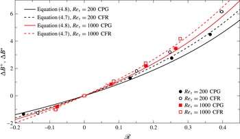
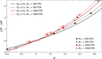
is large enough for the friction law (4.5) to hold. This can easily be tested with our DNS data, as shown in figure 11, where data from the large-box simulations already considered in figure 10 are used. The uncertainty on
 $\unicode[STIX]{x0394}B$
has been computed at 95 % confidence level through partial-derivative-based Gaussian error propagation of the uncertainties on
 $C_{f}$
and
 $C_{f,0}$
, similarly to what has been done for
 $\mathscr{R}$
in § 2.3, but using the definitions of
 $\unicode[STIX]{x0394}B$
given in (4.7) and (4.8). At
 $Re_{\unicode[STIX]{x1D70F}}=1000$
the agreement is excellent, for both the CPG and CFR cases. The agreement is less good at
 $Re_{\unicode[STIX]{x1D70F}}=200$
, and it is interesting to note that the largest deviation occurs for the CFR case with largest
 $\mathscr{R}$
at
 $Re_{\unicode[STIX]{x1D70F}}=200$
, i.e. for the case possessing the lowest actual
 $Re_{\unicode[STIX]{x1D70F}}$
(namely
 $Re_{\unicode[STIX]{x1D70F}}=173$
). It comes as no surprise that, at such low
 $Re_{\unicode[STIX]{x1D70F}}$
, the assumptions underlying the friction law (4.5), which implies that the flow rate is well approximated by the wall-normal integral of the logarithmic velocity profile, do not apply in full.


Quite surprisingly, a very similar picture is observed in figure 12 for the small-box simulations, where the mean velocity profile in the outer region is expected to be affected by the size of the computational domain. Of course, the five CPG data points are not contained in table 1, which lists only CFR cases for the small-box dataset, and have been produced on purpose. Despite the larger statistical uncertainty of
 $\mathscr{R}$
and the indeed quite small extent of the healthy logarithmic region, which translates into a non-negligible uncertainty for
 $\unicode[STIX]{x0394}B$
, the data at
 $Re_{\unicode[STIX]{x1D70F}}=1000$
agree fairly well with (4.7) and (4.8), while those at
 $Re_{\unicode[STIX]{x1D70F}}=200$
do not, because
 $Re$
is too low, in analogy with the corresponding data from the large-box simulations.
The evidence that (4.7) and (4.8) describe well the relationship among
 $C_{f,0}$
(hence
 $Re_{\unicode[STIX]{x1D70F}}$
),
 $\mathscr{R}$
and
 $\unicode[STIX]{x0394}B$
at sufficiently high
 $Re$
implies that these equations also describe the effect of
 $Re$
on
 $\mathscr{R}$
, provided information is known about the
 $Re$
dependence of
 $\unicode[STIX]{x0394}B$
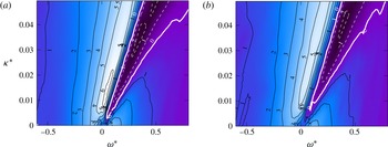
. This information can be educed from the small-box database introduced in § 2.1. Figure 13 shows the map of
 $\unicode[STIX]{x0394}B^{\ast }$
at
 $Re_{\unicode[STIX]{x1D70F}}=200$
and
 $1000$
, in actual viscous scaling at
 $A^{\ast }=12$
. Instead of measuring
 $\unicode[STIX]{x0394}B$
from the velocity profiles,
 $\unicode[STIX]{x0394}B$
is computed here ex post from the independently validated values of
 $\mathscr{R}$
through (4.7). In this way, the computed value of
 $\unicode[STIX]{x0394}B$
matches the measured value at
 $Re_{\unicode[STIX]{x1D70F}}=1000$
, while it is consistently slightly smaller at
 $Re_{\unicode[STIX]{x1D70F}}=200$
(see figures 11 and 12). This estimate of
 $\unicode[STIX]{x0394}B$
at low
 $Re$
is still meaningful, as it can be interpreted to represent the
 $\unicode[STIX]{x0394}B$
value free from the low-
 $Re$
effects that are due to deviations from the predictions of the friction law.
Map of
 $\unicode[STIX]{x0394}B^{\ast }$
for streamwise-travelling waves at
 $A^{\ast }=12$
, for
 $Re_{\unicode[STIX]{x1D70F}}=200$
(a) and
 $Re_{\unicode[STIX]{x1D70F}}=1000$
(b). Contours are spaced by 1, and negative contours are dashed. The thick white line corresponds to
 $\unicode[STIX]{x0394}B^{\ast }=0$
.

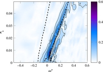
Map of the difference between
 $\unicode[STIX]{x0394}B^{\ast }$
at
 $Re_{\unicode[STIX]{x1D70F}}=200$
and
 $\unicode[STIX]{x0394}B^{\ast }$
at
 $Re_{\unicode[STIX]{x1D70F}}=1000$
for
 $A^{\ast }=12$
, relative to the reference value
 $B=5.2$
, obtained for the uncontrolled flow at
 $Re_{\unicode[STIX]{x1D70F}}=200$
. Contour lines are from 0.06 to 0.6 in 10 steps. The thick dashed line marks the region of large drag reduction, i.e.
 $\mathscr{R}>0.3$
, at
 $Re_{\unicode[STIX]{x1D70F}}=200$
.

When compared to the two maps in figure 5, where
 $\mathscr{R}$
is observed to decrease significantly across the whole plane, the two maps of
 $\unicode[STIX]{x0394}B^{\ast }$
appear much more similar, if exception is made for a localized change near the origin of the
 $(\unicode[STIX]{x1D714}^{\ast },\unicode[STIX]{x1D705}^{\ast })$
plane. Figure 14 emphasizes the relative changes of
 $\unicode[STIX]{x0394}B^{\ast }$
with
 $Re$
, by plotting the difference between the two previous maps, i.e. the pointwise difference between
 $\unicode[STIX]{x0394}B^{\ast }$
at
 $Re_{\unicode[STIX]{x1D70F}}=200$
and
 $\unicode[STIX]{x0394}B^{\ast }$
at
 $Re_{\unicode[STIX]{x1D70F}}=1000$
, normalized by the reference value
 $B=5.2$
of the uncontrolled flow at
 $Re_{\unicode[STIX]{x1D70F}}=200$
. Figure 14 strengthens the previous claim that
 $\unicode[STIX]{x0394}B$
is roughly constant with
 $Re$
, once low-
 $Re$
effects are discarded. In fact, except for a thin strip located on the right of the drag-reduction ridge, the variation of
 $\unicode[STIX]{x0394}B^{\ast }$
with
 $Re$
is essentially zero. In this region, which includes the whole area of large drag reduction except its right boundary, the function
 $\unicode[STIX]{x0394}B^{\ast }(\unicode[STIX]{x1D714}^{\ast },\unicode[STIX]{x1D705}^{\ast })$
is determined solely by the control parameters, and (4.6) can be used to describe the decrease of
 $\mathscr{R}$
with
 $Re$
. The thin strip, on the other hand, is a low-
 $Re$
effect that represents a non-trivial feature specific to the present control technique.
Although this is not enough for the ultimate demonstration that
 $\unicode[STIX]{x0394}B^{\ast }$
does not depend on
 $Re$
, the scenario depicted above is more than reasonable, and is reinforced by the parallel made with riblets. Moreover, additional data exist to support it. For example, in their figure 16 Hurst et al. (Reference Hurst, Yang and Chung2014) plot mean streamwise velocity profiles for channel flow modified by stationary waves at
 $\unicode[STIX]{x1D714}^{+}=0$
and
 $\unicode[STIX]{x1D705}^{+}=0.008$
with
 $A^{+}=12$
and
 $Re_{\unicode[STIX]{x1D70F}}=\{200,400,800,1600\}$
. By comparison with the reference profiles, they report
 $\unicode[STIX]{x0394}B^{+}=\{7.6,6.2,5.5,5.0\}$
, respectively. The changes clearly are progressively decreasing as
 $Re$
is increased. Moreover, it should be noted that the point at
 $\unicode[STIX]{x1D714}^{+}=0$
and
 $\unicode[STIX]{x1D705}^{+}=0.008$
lies in the small area where the residual
 $Re$
effect is maximum (see our figure 14) and some change
 $\unicode[STIX]{x0394}B$
is expected. Lastly, Hurst et al. (Reference Hurst, Yang and Chung2014) adopted a reference viscous scaling, which by itself induces a change in
 $\unicode[STIX]{x0394}B$
: as
 $Re$
increases,
 $\mathscr{R}$
shrinks,
 $u_{\unicode[STIX]{x1D70F}}/u_{\unicode[STIX]{x1D70F},0}$
increases and the actual forcing amplitude
 $A^{\ast }$
decreases. Hence, the data from Hurst et al. (Reference Hurst, Yang and Chung2014) are compatible with the present work in suggesting that, for a large enough
 $Re$
, the function
 $\unicode[STIX]{x0394}B(\unicode[STIX]{x1D714}^{\ast },\unicode[STIX]{x1D705}^{\ast })$
characterizes the forcing, and becomes constant with
 $Re$
above a threshold value. We estimate this minimum
 $Re$
to be
 $Re_{\unicode[STIX]{x1D70F}}\approx 2000$
.
5 Concluding discussion
In this study a large drag-reduction DNS database has been produced for a turbulent plane channel flow subject to a spanwise forcing. A total of 4020 simulations have been used to describe how increasing the value of the Reynolds number from
 $Re_{\unicode[STIX]{x1D70F}}=200$
to
 $Re_{\unicode[STIX]{x1D70F}}=1000$
affects drag reduction, and to propose a rationale behind the observed performance deterioration. To the authors’ knowledge, this is the first study on spanwise forcing that includes a wide range of forcing amplitudes, as well as constant pressure gradient (CPG) data at different values of
 $Re$
. The large size of the numerical study has been made possible thanks to the use of relatively small computational domains, which at the same time also constitutes its main limitation. This strategy has already been proved by Gatti & Quadrio (Reference Gatti and Quadrio2013) to successfully provide useful and accurate information about changes in friction drag. Moreover, the numerical results and the main conclusions are corroborated by 20 additional cases where a large computational domain is employed. The main findings of this study can summarized as follows.
-
(i) The existing information regarding spanwise forcing has been significantly extended. Thanks to the depth of the numerical study, the maximum net saving rate of streamwise-travelling waves at
$Re_{\unicode[STIX]{x1D70F}}=200$
is
$0.31\pm 0.021$
, a condition at which they produce a drag reduction of
$0.382\pm 0.002$
and a gain of
$5.3\pm 0.24$
; these figures become
$0.19\pm 0.002$
,
$0.255\pm 0.02$
and
$3.9\pm 0.31$
at
$Re_{\unicode[STIX]{x1D70F}}=1000$
. We have shown how the scaling choices (viscous units based on the reference friction velocity, i.e. ‘
$+$
’ scaling, or viscous units based on the actual friction velocity of the drag-reduced flow, i.e. ‘
$\ast$
’ scaling) impact the results, and the ensuing differences have been discussed. Though less practicable to implement, actual
$\ast$
scaling has been shown to be more advantageous to describe phenomena and quantities that are expected to scale in viscous units, such as the shape of the mean velocity profile in the viscous sublayer or the shape of skin-friction drag-reduction maps at different
$Re$
. -
(ii) The deterioration of performance with
$Re$
has been confirmed, in agreement with the majority of existing data. The often assumed but arbitrary power-law decrease of drag reduction with
$Re$
, i.e.
$\mathscr{R}\sim Re_{\unicode[STIX]{x1D70F}}^{-\unicode[STIX]{x1D6FE}}$
, yields values of the exponent
$\unicode[STIX]{x1D6FE}$
that vary strongly across the space of control parameters. The lack of rationale for a power-law dependence is such that a
$\unicode[STIX]{x1D6FE}$
-based extrapolation at higher
$Re$
of existing data should be regarded as potentially unreliable. -
(iii) The classic argument linking the skin-friction drag changes of a rough wall to the vertical shift
$\unicode[STIX]{x0394}B$
of the logarithmic portion of the mean velocity profile has been shown to apply to the case of spanwise forcing. A nonlinear expression has been derived that can be specialized to the CFR or CPG cases. As for drag-reducing riblets, characterizing drag reduction through
$\unicode[STIX]{x0394}B$
is more informative than the simple statement of ‘percentage drag reduction’. Indeed,
$\unicode[STIX]{x0394}B$
already contains the necessary
$Re$
dependence through the friction law and, if the control parameters in actual units are constant, it does not significantly change once
$Re$
is above the threshold where the mean velocity profile features a well-defined logarithmic region, and the validity of the friction law (4.5) is ensured. -
(iv) Under the assumption that
$\unicode[STIX]{x0394}B^{\ast }$
measured in the present work at
$Re_{\unicode[STIX]{x1D70F}}=1000$
is already
$Re$
-independent, equation (4.6) can be used to extrapolate drag reduction at higher
$Re_{\unicode[STIX]{x1D70F}}$
, as done in figure 15(a), showing that a drag reduction of
$\mathscr{R}=0.5$
at
$Re_{\unicode[STIX]{x1D70F}}=1000$
translates into
$\mathscr{R}=0.34$
at
$Re_{\unicode[STIX]{x1D70F}}=10^{5}$
. The decrease is still significant but not as dramatic as the low-
$Re$
evidence suggests: this can be easily appreciated by looking at the dashed line, which describes
$\mathscr{R}\sim Re_{\unicode[STIX]{x1D70F}}^{-\unicode[STIX]{x1D6FE}}$
with
$\unicode[STIX]{x1D6FE}=0.20$
. The whole drag-reduction map at
$A^{\ast }=12$
is extrapolated from
$Re_{\unicode[STIX]{x1D70F}}=1000$
to
$Re_{\unicode[STIX]{x1D70F}}=10^{5}$
in figure 15(b). The maximum drag reduction in the plane reduces from 0.34 to 0.23, which is still a sizeable amount considering the two decades increase of
$Re$
. -
(v) While we are not in a position to make a claim of generality, we believe that the line of reasoning developed in this paper for spanwise forcing might apply to other wall-based active control techniques, as long as they do not disrupt the shape of the mean velocity profile. The relation among
$\unicode[STIX]{x0394}B$
,
$C_{f,0}$
and
$\mathscr{R}$
and the observation that
$\unicode[STIX]{x0394}B$
becomes
$Re$
-independent provide an unbiased framework to describe the effect of the Reynolds number on turbulent drag reduction obtained via wall-based control. For riblets,
$\unicode[STIX]{x0394}B$
depends on the riblet geometry alone. For spanwise forcing, a given set of control parameters determines the properties of the generalized Stokes layer (Quadrio & Ricco Reference Quadrio and Ricco2011), whose features, such as its thickness (Quadrio & Ricco Reference Quadrio and Ricco2011) or spanwise shear stress at a certain wall distance (Yakeno et al.
Reference Yakeno, Hasegawa and Kasagi2014), determine the shift
$\unicode[STIX]{x0394}B$
or, equivalently, the
$Re$
-dependent drag-reduction rate
$\mathscr{R}$
according to (4.7) or (4.8). Hence, the comparison between wall-based control at different Reynolds numbers should be made in terms of
$\unicode[STIX]{x0394}B$
, not of
$\mathscr{R}$
. -
(vi) Although the present results are sound from a quantitative standpoint, we believe that an accurate DNS study of the drag-reduction properties of the travelling waves at higher
$Re$
is still needed. Such an ultimate study would be forcedly less vast than the present one, but could be designed by leveraging the available information. The view presented in this paper, with its Achilles’ heel of being based on small-box simulations, will surely benefit from an independent confirmation. Moreover,
$Re_{\unicode[STIX]{x1D70F}}=1000$
is still smaller than the minimal
$Re$
at which the values of
$\unicode[STIX]{x0394}B$
are expected to become fully
$Re$
-independent. We stress that this minimal
$Re$
, suggested to be
$Re_{\unicode[STIX]{x1D70F}}\approx 2000$
, is rather smaller than the minimal
$Re$
required for the mean velocity profile to show an incipient true logarithmic region, observed for example by Lozano-Durán & Jiménez (Reference Lozano-Durán and Jiménez2014a
) at
$Re_{\unicode[STIX]{x1D70F}}=4200$
and by Lee & Moser (Reference Lee and Moser2015) at
$Re_{\unicode[STIX]{x1D70F}}=5200$
. Anyway, this ultimate study is all that is left to do for the complete characterization of the drag-reduction capabilities of the travelling waves, at any (high enough)
$Re$
.


Extrapolation of drag-reduction data from
 $Re_{\unicode[STIX]{x1D70F}}=1000$
to
 $Re_{\unicode[STIX]{x1D70F}}=100\,000$
. (a) Continuous lines are prediction by (4.6), while the dashed line shows a decrease of
 $\mathscr{R}\propto Re_{\unicode[STIX]{x1D70F}}^{-0.2}$
. (b) Extrapolated drag-reduction map at
 $Re_{\unicode[STIX]{x1D70F}}=10^{5}$
for
 $A^{\ast }=12$
; lines and symbols as in figure 3. The white shaded area is excluded from the contour plot as there
 $\unicode[STIX]{x0394}B$
is found to vary between
 $Re_{\unicode[STIX]{x1D70F}}=200$
and
 $Re_{\unicode[STIX]{x1D70F}}=1000$
.

Although so far we have deliberately avoided mentioning turbulent structures, by strictly limiting our discussion to the simplest first-order statistics, we would like to close this paper with a remark of a more general nature.
On a fundamental level, the dependence of
 $C_{f}$
upon
 $Re$
may be seen to reflect the variable extension of the different portions of a turbulent wall flow, in particular the inner and the outer layers, and the way they interact with each other. The importance of the inner layer has probably been overemphasized in the last decades: indeed, at the low values of
 $Re$
typical of most studies addressing near-wall turbulence and its control, the inner layer occupies a significant portion of the whole flow. At higher
 $Re$
, however, the wall-normal extension of the inner layer becomes progressively smaller with respect to the outer layer, and at application-level
 $Re$
most of the boundary layer is just outer layer. It is also known, thanks for example to the FIK identity (Fukagata, Iwamoto & Kasagi Reference Fukagata, Iwamoto and Kasagi2002), that the portion of Reynolds shear stresses located in the outer layer carries an increasing contribution to the skin-friction coefficient as
 $Re$
increases. These Reynolds stresses are due to the very large turbulent structures (Ganapathisubramani, Longmire & Marusic Reference Ganapathisubramani, Longmire and Marusic2003; Guala, Hommema & Adrian Reference Guala, Hommema and Adrian2006) that populate the outer layer and modulate the smaller structures residing near the wall (Brown & Thomas Reference Brown and Thomas1977; Ganapathisubramani et al.
Reference Ganapathisubramani, Hutchins, Monty and Marusic2012; Lozano-Durán & Jiménez Reference Lozano-Durán and Jiménez2014b
). This modulation has been confirmed also in the case of drag-reducing flows (see e.g. Touber & Leschziner Reference Touber and Leschziner2012).
Those present results that are computed in small computational domains only partially represent the large structures of the flow. In fact, only those structures whose width fits into the domain are actually well resolved (Flores & Jiménez Reference Flores and Jiménez2010), with their longer streamwise extent ending up as indefinitely long owing to the periodic boundary conditions. Even though physically incorrect, these large scales still interact healthily with the well-resolved smaller scales, as pointed out by Lozano-Durán & Jiménez (Reference Lozano-Durán and Jiménez2014a
), who observed that small computational boxes with spanwise width larger than
 $L_{z}/h=\unicode[STIX]{x03C0}/2$
still yield correct low-order statistics. However, the present values of
 $L_{z}$
are well below this threshold, so that a significant part of the large scales, which at
 $Re_{\unicode[STIX]{x1D70F}}=1000$
already carry a non-negligible contribution to Reynolds stresses and hence to turbulent drag (Ganapathisubramani et al.
Reference Ganapathisubramani, Longmire and Marusic2003), are not resolved. This explains the significant deviations of the values of
 $C_{f}$
from the correct value observed for the uncontrolled flow. Nonetheless, the nearly correct prediction of changes in
 $C_{f}$
, i.e. drag reduction, via small-box simulations suggests that the large outer structures might not significantly interfere with the working mechanism of wall-based strategies for drag reduction. The control action takes place at the wall and targets turbulence in the very vicinity of the wall, and the largest eddies that attach to the wall (Lozano-Durán & Jiménez Reference Lozano-Durán and Jiménez2014b
) simply perceive a modified inner layer with a lower mean shear. In other words, the control performance deterioration occurs mainly because of the geometric effect of the shrinking near-wall region, which contributes progressively less to turbulent drag. The large structures, which contribute to turbulent friction via the Reynolds shear stress produced in the outer region, do not directly jeopardize the drag-reducing action of the wall-based spanwise forcing. This does not preclude that, should a control technique succeed in targeting the outer structures directly, additional turbulent drag reduction at high
 $Re$
could be obtained. The present results thus blend nicely with the result, presented by Iwamoto et al. (Reference Iwamoto, Fukagata, Kasagi and Suzuki2005), that artificially removing the turbulent fluctuations in a thin wall layer of constant thickness when measured in inner units produces a reduction of friction which is unexpectedly robust with respect to the increase in
 $Re$
. There is thus no need to control the outer structures directly to achieve drag reduction at high
 $Re$
, although of course being able to do so would yield additional benefits.
Acknowledgements
Support through DFG project FR2823/5-1 is gratefully acknowledged. Preliminary versions of this work have been presented by M.Q. at the ERCOFTAC Flow Control and Drag Reduction meeting in Cambridge, April 2015, and by D.G. at the XV Euromech Turbulence Conference (ETC) in Delft, August 2015. Computing time has been provided by the Italian Supercomputing Center CINECA (through a LISA 2013 grant), and by the computational resource ForHLR Phase I funded by the Ministry of Science, Research and the Arts, Baden-Württemberg and DFG (‘Deutsche Forschungsgemeinschaft’). S. Chernyshenko is thanked for an interesting discussion on the topic in Lyon during ETC 2013.
Appendix
In § 4.2, equations (4.7) and (4.8) reciprocally linking drag reduction, the friction coefficient and
 $Re$
, have been deduced under the assumption that the von Kármán constant
 $k$
is independent of
 $Re$
, and the intercept
 $B_{1}$
is negligible for channel flows. The validity of these assumptions can be verified by measuring
 $k$
,
 $B$
and
 $B_{1}$
for the whole set of 20 large-box simulations by fitting the log law (4.4) to the mean velocity profiles shown in figure 10. The results are summarized in table 2.
The extrema of the least-squares fitted region in wall-normal direction are chosen in such a way that the width of the fitted region is as large as possible, while keeping a correlation coefficient
 $r^{2}\geqslant 0.9995$
(where
 $r^{2}=1$
means perfect fit). The same procedure was employed by Lee & Moser (Reference Lee and Moser2015) with
 $r^{2}=0.9999$
at
 $Re_{\unicode[STIX]{x1D70F}}=5186$
. The present, slightly lower threshold for
 $r^{2}$
descends from the lower
 $Re$
, which implies a shorter logarithmic region. The lower bound of the fit is set at least 10 wall units past the relative minimum of the diagnostic function
 $y^{+}\,\text{d}\langle u\rangle ^{+}/\text{d}y^{+}$
. Note that choosing the range for this curve fit is somewhat arbitrary (Lee & Moser Reference Lee and Moser2015).
The near-wall intercept
 $B$
is a function of
 $k$
and is very sensitive to small variation thereof. Thus, small uncertainties on
 $k$
due to the arbitrariness of the log-region range strongly affect
 $B$
and make its measure not readily comparable among different simulations. Therefore, the numerical value of
 $k$
in the controlled cases is kept equal to the uncontrolled value while the validity of the aforementioned assumption is verified indirectly by monitoring that the change in
 $k$
is smaller than 0.01. In fact, the value of
 $k$
is known to weakly influence the way the logarithmic and defect laws (4.3) and (4.4) approximate the mean velocity profile (Del Álamo et al.
Reference Del Álamo, Jiménez, Zandonade and Moser2004).
Values of the von Kármán constant
 $k$
, the intercepts
 $B^{\ast }$
and
 $B_{1}^{\ast }$
, the drag-reduction rate
 $\mathscr{R}$
and its uncertainty
 $\unicode[STIX]{x03B4}\mathscr{R}$
, for the 20 large-box cases detailed in table 1, identified with their control parameters and their actual values of
 $Re$
.