

Introduction
Whole-brain studies of intrinsic functional connectivity (iFC) may elucidate dysfunctional circuitry in bipolar disorder (BD) that spans widespread neural regions, mediates diverse neuropsychological impairments (Robinson et al. Reference Robinson, Thompson, Gallagher, Goswami, Young, Ferrier and Moore2006; Bora et al. Reference Bora, Yucel and Pantelis2009; Kurtz & Gerraty, Reference Kurtz and Gerraty2009), and manifests similarly in youths and adults with the illness. Here, we use a recently developed, data-driven, whole-brain approach (Gotts et al. Reference Gotts, Simmons, Milbury, Wallace, Cox and Martin2012) to compare iFC in youths and adults with v. without BD.
Prior iFC studies in BD suggest the importance of network-based approaches (Vargas et al. Reference Vargas, López-Jaramillo and Vieta2013). However, most such studies test group differences in iFC by pre-selecting a limited number of anatomic nodes, or seeds, often including the amygdala (Anand et al. Reference Anand, Li, Wang, Lowe and Dzemidzic2009; Dickstein et al. Reference Dickstein, Gorrostieta, Ombao, Goldberg, Brazel, Gable, Kelly, Gee, Zuo, Castellanos and Milham2010; Chai et al. Reference Chai, Whitfield-Gabrieli, Shinn, Gabrieli, Nieto Castanon, McCarthy, Cohen and Ongur2011; Anticevic et al. Reference Anticevic, Brumbaugh, Winkler, Lombardo, Barrett, Corlett, Kober, Gruber, Repovs, Cole, Krystal, Pearlson and Glahn2013, Reference Anticevic, Yang, Savic, Murray, Cole, Repovs, Pearlson and Glahn2014; Mamah et al. Reference Mamah, Barch and Repovs2013; Torrisi et al. Reference Torrisi, Moody, Vizueta, Thomason, Monti, Townsend, Bookheimer and Altshuler2013; Favre et al. Reference Favre, Baciu, Pichat, Bougerol and Polosan2014). While intriguing results have emerged, findings are inconsistent, even in studies investigating the same anatomic region (for a review, see Torrisi et al. Reference Torrisi, Moody, Vizueta, Thomason, Monti, Townsend, Bookheimer and Altshuler2013). Data-driven methods may address major limitations due to seed selection in these studies (Smith et al. Reference Smith, Miller, Salimi-Khorshidi, Webster, Beckmann, Nichols, Ramsey and Woolrich2011) and, in a standardized fashion, identify networks with aberrant iFC across the brain.
Indeed, several whole-brain, data-driven investigations report widespread iFC abnormalities in BD (online Supplementary Table S1), suggesting large-scale network dysfunction in BD (e.g. temporal and default mode network dysfunction; Calhoun et al. Reference Calhoun, Maciejewski, Pearlson and Kiehl2008). For example, an analysis of global connectivity among 266 anatomic nodes suggests diffuse, decreased functional connectivity in BD (Argyelan et al. Reference Argyelan, Ikuta, Derosse, Braga, Burdick, John, Kingsley, Malhotra and Szeszko2014). Studies using group-level independent components analysis (ICA) find dysconnectivity in BD within and between functional networks throughout the brain (Meda et al. Reference Meda, Gill, Stevens, Lorenzoni, Glahn, Calhoun, Sweeny, Tamminga, Keshavan, Thaker and Pearlson2012; Wu et al. Reference Wu, Lu, Passarotti, Wegbreit, Fitzgerald and Pavuluri2013; Rashid et al. Reference Rashid, Damaraju, Pearlson and Calhoun2014; Du et al. Reference Du, Pearlson, Liu, Sui, Yu, He, Castro and Calhoun2015). These studies implicate corticostriatal, late visual, sensorimotor, affective, and default mode network dysfunction in BD. Similarly, whole-brain studies of various indicators of iFC, such as regional homogeneity, implicate BD-related network dysfunction involving the striatum, prefrontal cortex and precuneus, amongst other regions (Liu et al. Reference Liu, Li, Li, Wang, Tie, Wu, Zhou, Zhang, Dong, Yang and Wang2012; Xiao et al. Reference Xiao, Zhong, Lu, Gao, Jiao, Lu and Su2013; Gao et al. Reference Gao, Jiao, Lu, Zhong, Qi, Lu, Xiao, Yang, Lu and Su2014; Lu et al. Reference Lu, Jiao, Zhong, Gao, Xiao, Liu, Lin, Cheng, Luo, Xu, Lu and Su2014; Wang et al. Reference Wang, Zhong, Jia, Zhou, Wang, Pan and Huang2015). In sum, data-driven studies of iFC in BD implicate dysconnectivity across the brain involving multiple networks. However, the number of data-driven, whole-brain iFC studies in BD remains limited, and more studies are needed.
Moreover, a whole-brain iFC analysis may identify networks that are dysfunctional in BD and in which the abnormality varies developmentally. Disruptions in functional network development have been associated with other mental disorders, such as major depressive disorder (Uddin et al. Reference Uddin, Suprekar and Menon2010). However, no studies have directly tested developmental associations between iFC and BD. Several studies find iFC abnormalities in pediatric BD (Dickstein et al. Reference Dickstein, Gorrostieta, Ombao, Goldberg, Brazel, Gable, Kelly, Gee, Zuo, Castellanos and Milham2010; Wu et al. Reference Wu, Lu, Passarotti, Wegbreit, Fitzgerald and Pavuluri2013; Xiao et al. Reference Xiao, Zhong, Lu, Gao, Jiao, Lu and Su2013; Gao et al. Reference Gao, Jiao, Lu, Zhong, Qi, Lu, Xiao, Yang, Lu and Su2014; Lu et al. Reference Lu, Jiao, Zhong, Gao, Xiao, Liu, Lin, Cheng, Luo, Xu, Lu and Su2014), and these abnormalities are similar to those described in adults with BD in that they are widespread. In the present study, we address this important question by testing the effects of age on iFC dysconnectivity in BD.
Recently, Gotts et al. (Reference Gotts, Simmons, Milbury, Wallace, Cox and Martin2012) developed data-driven procedures, well suited to addressing these questions. Like other such methods, these procedures improve upon seed-based approaches by empirically deriving group-based differences in network connectivity. Complementary to other whole-brain approaches, this procedure has a relative strength in its high anatomic specificity. Here, we apply this procedure to a sample of patients with BD, ages 10–50 years. We expect this whole-brain approach to identify novel regions with aberrant iFC in BD and their organization into functional circuits, while assessing differences in iFC between youths and adults with BD.
Method
Participants
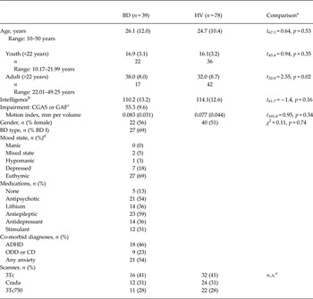
This Institutional Review Board-approved study was conducted at the National Institute of Mental Health (NIMH). Adult participants gave written informed consent; youth and their parents provided assent/consent prior to study participation. In all, 39 participants with BD (ages 10–50 years) completed a resting-state functional magnetic resonance imaging (fMRI) scan on one of three GE 3T scanners. BD participants were matched by scanner to 78 healthy volunteers (HV) (Table 1; online Supplementary Table S2). In this study the boundaries of age category (youth v. adult) were at the median split of the entire sample at 22 years old. Using a median split allowed us to maintain balance between diagnostic groups and age categories when adjusting for scanner effects. Patients in the youth group were mid-adolescent (mean = 16.9, s.d. = 3.1 years old), with an average age of onset at 10.2 (s.d. = 3.4) years, and those in the adult group were 38.0 (s.d. = 8.0) years old with an average age of onset at 19.7 (s.d. = 9.1) years.
Participant characteristics and scanning parameters

Data are given as mean (standard deviation) unless otherwise indicated.
BD, Bipolar disorder; HV, healthy volunteer; CGAS, Children's Global Assessment Scale; GAF, Global Assessment of Functioning Scale; ADHD, attention-deficit/hyperactivity disorder; ODD, oppositional defiant disorder; CD, conduct disorder; n.a., not applicable; IQ, intelligence quotient; YMRS, Young Mania Rating Scale; CDRS, Children's Depression Rating Scale; SIGH-SAD, Structured Interview Guide for the Hamilton Depression Rating Scale, Seasonal Affective Disorders Version.
a Comparisons by Welch t test (BD–HV) or χ 2 test.
b IQ estimates within 2 years of scanning, missing for five BD and five HV.
c CGAS or GAF missing for 11 BD.
d Mood state was determined by YMRS, CDRS and SIGH-SAD score. Depressed state limits were YMRS ⩽12 and CDRS ⩾40 or SIGH-SAD ⩾20, hypomanic limits were YMRS >12 but <26 and CDRS <40 or SIGH-SAD <20, mania limits were YMRS ⩾26 and CDRS <40 or SIGH-SAD <20, and mixed state limits were YMRS >12 and CDRS ⩾40 or SIGH-SAD ⩾20. Complete mood state data were missing for two BD.
e Groups were balanced across scanner.
Five additional BD patients completed scans that were excluded from analysis due to motion (limits described below). Data from 14 BD patients were reported previously in a study of amygdala iFC (Stoddard et al. Reference Stoddard, Hsu, Reynolds, Brotman, Ernst, Pine, Leibenluft and Dickstein2014). Psychiatric diagnoses were determined by the Schedule for Affective Disorders and Schizophrenia for School-Age Children – Present and Lifetime Version (Kaufman et al. Reference Kaufman, Birmaher, Brent, Rao, Flynn, Moreci, Williamson and Ryan1997), the Structured Clinical Interview for the Diagnostic and Statistical Manual of Mental Disorders, Research Version, Patient Edition with Psychotic Screen (First et al. Reference First, Spitzer, Miriam and Williams2002), or the Diagnostic Interview for Genetic Studies (Nurnberger et al. Reference Nurnberger, Blehar, Kaufmann, York-Cooler, Simpson, Harkavy-Friedman, Severe, Malaspina and Reich1994). Interviews were administered by master's- or doctoral-level clinicians trained to reliability. BD inclusion criteria were meeting full Diagnostic and Statistical Manual of Mental Disorders, 4th edition (DSM-IV; American Psychiatric Association, 2000) criteria for BD I or II. HV inclusion criteria were the absence of Axis I psychopathology, first-degree relatives with a mood disorder, or psychotropic medication use. Exclusion criteria for all groups were chronic or active medical conditions, autism spectrum disorder, substance use within the last 2 months, head trauma and intelligence quotient (IQ) <80.
Behavioral measures
Mood was assessed within 48 h of scan acquisition. All patients were assessed with the Young Mania Rating Scale (Young et al. Reference Young, Biggs, Ziegler and Meyer1978). Depressive symptoms were measured with the Children's Depression Rating Scale (Poznanski et al. Reference Poznanski, Cook and Carroll1979) in those younger than 18 years or with the Structured Interview Guide for the Hamilton Depression Rating Scale, Seasonal Affective Disorders Version (Williams et al. Reference Williams, Link, Rosenthal and Terman1988) in adults. We measured 6-month impairment with the Children's Global Assessment Scale (Shaffer et al. Reference Shaffer, Gould, Brasic, Ambrosini, Fisher, Bird and Aluwahlia1983) in those younger than 18 years or with the Global Assessment of Functioning Scale (Endicott et al. Reference Endicott, Spitzer, Fleiss and Cohen1976).
Image acquisition
Due to scanners being decommissioned at the National Institutes of Health (NIH) Nuclear Magnetic Resonance (NMR) Research Center, MRI images were acquired on three General Electric 3.0 Tesla scanners (Table 1). Diagnostic groups were balanced across scanner, maintaining a fixed ratio of one BD for every two HV participants on each scanner. This 2-to-1 matching allowed us to eliminate any group differences due to different proportions of subjects studied on a particular scanner. For a good estimate of the covariate effects of scanner, we accrued at least 30 participants per scanner. Resting-state fMRI scans were acquired while participants passively viewed a fixation cross for 6 min. Blood oxygen level-dependent (BOLD) signals were measured by echoplanar imaging (EPI) with the same parameters across scanners (flip angle = 90°, echo time = 30 ms, repetition time = 2.0 s, 180 volumes, acquisition time = 6 min, field of view = 192 mm, and acquisition voxel size = 3 × 3 × 4 mm). For anatomic registration and normalization, high-resolution, T1-weighted MPRAGE images were collected as follows. For scanner 1: flip angle = 7°, minimum full echo time, inversion time = 425 ms, acquisition voxel size = 1 mm isotropic; for scanners 2 and 3: flip angle = 6°, minimum full echo time, inversion time = 725 ms, acquisition voxel size = 0.86 × 1.15 × 1.20 mm.
Subject-level image processing
All images were processed using FreeSurfer (Reuter et al. Reference Reuter, Schmansky, Rosas and Fischl2012) and Analysis of Functional Neuroimages (AFNI; Cox, Reference Cox1996) resting-state image processing streams (Jo et al. Reference Jo, Saad, Simmons, Milbury and Cox2010, Reference Jo, Gotts, Reynolds, Bandettini, Cox and Saad2013) to minimize the effect of motion, physiological and hardware noise. Anatomic images were skull stripped and segmented via FreeSurfer to create an anatomic registration base and all of the standardized, anatomically defined masks in the analyses described below. EPI images were processed by excising the first four volumes, attenuating outlying time points for each voxel's BOLD time series to within four standard deviations of the mean, correcting for slice timing, registering to the subject's first pre-steady-state volume, and smoothing by a 4 mm full-width at half maximum (FWHM) Gaussian kernel.
Estimated physiological, motion and hardware noise were removed from EPI images via general linear modeling (GLM) regression with the following parameters: a cubic detrending polynomial, 12 motion parameters (the six translational and rotational parameters from volume registration and their six derivatives), the first three principal components (PCs) of all voxel time series within a combined white matter (WM) and cerebrospinal fluid (CSF) mask (anatomic CompCor; Behzadi et al. Reference Behzadi, Restom, Liau and Liu2007), mean CSF signal, and locally averaged WM signal (within a sphere radius of 25 mm) as implemented in the ANATICOR method (Jo et al. Reference Jo, Saad, Simmons, Milbury and Cox2010, Reference Jo, Gotts, Reynolds, Bandettini, Cox and Saad2013). All tissue-based nuisance signals were derived prior to spatial smoothing and after mask erosion (by one voxel) in order to prevent partial volume effects with gray matter signals. EPI volumes were censored from this GLM regression by three criteria: (i) any volume with a motion shift, defined as movement exceeding Euclidean distance of 0.3 mm from its preceding volume; (ii) any volume immediately preceding such a motion shift; and (iii) any volume with a large fraction (>10%) of outlying time points. To prevent excessive intra-subject data loss and the inclusion of high motion individuals, subject-level exclusion occurred when more than 20% of volumes for that individual were censored. To attenuate physiological artifacts, we used tissue-based regressors instead of a bandpass filter due to frequency aliasing of cardiac and respiration cycles (Glover et al. Reference Glover, Li and Ress2000; Behzadi et al. Reference Behzadi, Restom, Liau and Liu2007; Birn et al. Reference Birn, Murphy and Bandettini2008). Time series fluctuations were in the frequency range of 0.003–0.25 Hz. A post-hoc analysis with a bandpass filter of 0.01–0.1 Hz did not alter group differences significantly (online Supplementary material).
Residuals from this regression represented neural BOLD signal time series used in the later stages of the analysis. In addition, a ‘global connectivity’ map was created for each individual (online Supplementary Fig. S1). To do so, in AFNI, each voxel's time series was correlated to the time series of all other voxels within a subject's brain tissue mask, defined by all brain regions except CSF and WM (Gotts et al. Reference Gotts, Simmons, Milbury, Wallace, Cox and Martin2012). For each voxel, the Fisher's z transform of the mean of the resultant Pearson's r values is a measure of global connectivity between the signal in that voxel and all other voxels in the mask.
Group-level analyses
Group analyses occurred in three stages (online Supplementary Fig. S2), following the standard protocol established and validated by Gotts et al. (Reference Gotts, Simmons, Milbury, Wallace, Cox and Martin2012). The first stage functionally identified clusters of voxels that differed in global connectivity based on diagnosis (BD v. HV), age category (youth v. adult) or their interaction. These clusters, or ‘primary locales’, reflect group differences in network connectivity (Buckner et al. Reference Buckner, Sepulcre, Talukdar, Krienen, Liu, Hedden, Andrews-Hanna, Sperling and Johnson2009; Gotts et al. Reference Gotts, Simmons, Milbury, Wallace, Cox and Martin2012; Di Martino et al. Reference Di Martino, Yan, Li, Denio, Castellanos, Alaerts, Anderson, Assaf, Bookheimer, Dapretto, Deen, Delmonte, Dinstein, Erti-Wagner, Fair, Gallagher, Kennedy, Keown, Keysers, Lainhart, Lord, Luna, Menon, Minshew, Monk, Mueller, Muller, Nebel, Nigg, O'Hearn, Pelphrey, Peltier, Rudie, Sunaert, Thioux, Tyszka, Uddin, Verhoeven, Wenderoth, Wiggins, Mostofsky and Milham2014). Thus, they constitute empirically defined, effective seed locations for further defining the nature of group differences in iFC. Analogous to descriptive post-hoc testing after an omnibus analysis of variance, the next stages of analysis describe the regionally specific differences in network connectivity that drive the observed differences in global connectivity. In the second stage we used the primary locales identified in the first stage as seeds in whole-brain voxel-wise tests of diagnosis, age category and their interaction on connectivity between these primary locales and other brain regions. These analyses generated a set of ‘secondary locales’ representing brain regions where iFC to the primary locales differed by diagnosis or age. Finally, a third stage organized these primary and secondary locales into functional networks, based on their correlation patterns.
First-stage group analysis: global connectivity
Each subject's global connectivity map was entered into analysis of covariance (ANCOVA) via the multivariate analysis program 3dMVM (Chen et al. Reference Chen, Adleman, Saad, Leibenluft and Cox2014) with main factors of diagnosis (HV v. BD), age category (youth v. adult), and diagnosis × age category interaction, along with nuisance covariates for scanner (1, 2 or 3) and a quantitative index of transient head motion per subject (i.e. the ‘motion index,’ calculated using the AFNI program @1dDiffMag). The motion index is comparable with mean framewise displacement (Power et al. Reference Power, Barnes, Snyder, Schlaggar and Petersen2012) and uses the framewise differences of the six motion parameter time series, taking the square root after summing over their corresponding variances (see also Gotts et al. Reference Gotts, Simmons, Milbury, Wallace, Cox and Martin2012; Meoded et al. Reference Meoded, Morrissette, Katipally, Schanz, Gotts and Floeter2014). Age category was defined by a median split of the sample at 22 years old. Results were thresholded voxel-wise at p < 0.001. Spatial cluster-size correction was used to generate whole-brain corrected results, which control for multiple tests across a group, based on the whole-brain gray matter mask via Monte Carlo simulation (the corrected α = 0.05, cluster-size threshold was 17 contiguous voxels, considering an initial p < 0.001 threshold and smoothness estimated from the data of x, y, z = 8.2,7.9,7.3 mm FWHM). Thus, diagnosis or age differences identified regions termed primary locales that were used as seeds in the second analysis stage.
Second-stage group analysis: seed testing
We then assessed group differences in iFC between each primary locale, used as seeds, and all other voxels within a group gray matter mask, as a function of diagnosis, age category, diagnosis × age category interaction, and nuisance covariates of scanner and motion index. Subject-level connectivity maps of Pearson's correlations were created between voxels’ time series and the mean time series of each primary locale. Subject-level connectivity maps were then Fisher z-transformed and entered into group analyses using the same 3dMVM ANCOVA test as in the first-stage group analysis. Results were thresholded voxel-wise at p < 0.001. Multiple testing was controlled by Monte Carlo cluster correction with a Bonferroni penalty for the number of seeds tested (i.e. α = 0.05 divided by the number of seeds determined the cluster-size threshold). Regions identified at this stage of the analyses are termed secondary locales, and, as in Gotts et al. (Reference Gotts, Simmons, Milbury, Wallace, Cox and Martin2012), we retained any region that yielded significant results in tests of two or more primary locales. To avoid excessively small secondary locales, we only included clusters ⩾20 contiguous voxels (>540 mm3). These procedures held the chance of a type I error below 0.05, over the entire family of tests conducted throughout the search process (i.e. correcting for both whole-brain testing and the number of seeds tested).
Third-stage group analysis: locale organization into functional networks
Diagnosis or age differences in iFC identified in the first two stages are not organized into functional networks. The third analytic stage derived such an organization based on patterns of correlations. For each subject, we calculated the pairwise Pearson's correlation between each of the primary or secondary locales’ mean time series and transformed these with Fisher's z (r z ). For each locale pair, we calculated the average partial r z within each diagnostic group, partialling out the effects of age category, diagnosis × age category interaction, scanner and motion index in 3dMVM. For each locale pair, partial r z values were averaged across the BD and HV groups, yielding a group-averaged locale × locale correlation matrix. The similarity of the locales with regard to their full pattern of correlation in this matrix was analysed with multidimensional scaling (MDS), principal component analysis (PCA), and k-means cluster analysis (see also Gotts et al. Reference Gotts, Simmons, Milbury, Wallace, Cox and Martin2012; Meoded et al. Reference Meoded, Morrissette, Katipally, Schanz, Gotts and Floeter2014). Given that MDS requires distances rather than correlations, correlations were first converted to distances using Matlab's pdist (Mathworks, Natick MA) function, using Euclidean distance. The number of clusters used in the k-means analysis was determined by the use of an ‘elbow’ plot, finding the best tradeoff of variance explained in the structure of the matrix and the model complexity (choice of k). This elbow was then checked against the scree plot of the eigenvalues in PCA, which shows how much variance in the matrix is explained by each PC. The internal consistency of MDS, PCA and cluster analyses was checked using scatterplots of MDS (best two-dimensional reduction of the locale × locale distance matrix) and PCA (first two PCs), with the k-means cluster membership shown in color. Agreement between different clustering methods is indicated by a clear spatial segregation of locales in MDS space that corresponds with the locales’ k-means membership coloring (as in Fig. 2b ; see also, Gotts et al. Reference Gotts, Simmons, Milbury, Wallace, Cox and Martin2012). The groupings derived through k-means served to define functionally related ‘networks’ of locales, with similar within-network patterns of correlation and weaker across-network patterns.
Post-hoc analyses
To examine the agreement of our functional networks with those in prior studies, we compared their topography with the Yeo et al. (Reference Yeo, Krienen, Sepulcre, Sabuncu, Lashkari, Hollinshead, Roffman, Smoller, Zollei, Polimeni, Fischl, Liu and Buckner2011) coarse parcellation of the human cortex into seven iFC networks. Using affine transformation, we aligned the parcellation's anatomic base to our study template. Using the resultant transformation matrix, we warped the parcellation into our study space and resampled it to our networks’ dimensions. Once aligned, we counted the number of cortical voxels in each of our networks that overlap with each of the seven parcellation networks.
For post-hoc analyses of group differences in the locale × locale matrix, the 3dMVM multivariate model used to estimate group partial r z was used to generate a matrix of standardized mean differences (Cohen's d) of the BD–HV r z contrast for each pair of locales. Additional post-hoc analyses on this matrix and the r z matrix in BD assessed the effects of mood state and medication use. Since different clinical measures were obtained to assess depression severity in adults v. youth, the scores were converted to T-scores and then combined for post-hoc analyses.
Ethical standards
All procedures contributing to this work comply with the ethical standards of the relevant national and institutional committees on human experimentation and with the Helsinki Declaration of 1975, as revised in 2008.
Results
Global connectivity
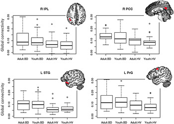
Across the brain, global connectivity was greater in BD than HV in four primary locales (Fig. 1; Table 2): (1) right inferior parietal lobule (Talairach–Tournoux cluster center xyz = 39.4, −48.6, 41.1; F 1,110 = 16.16, p < 0.001, η p 2 = 0.13); (2) right posterior cingulate (xyz = 2.0, −51.9, 25.8; F 1,110 = 16.38, p < 0.001, η p 2 = 0.13); (3) left superior temporal gyrus (xyz = −50.2, −11.5, −11.4; F 1,110 = 24.25, p < 0.001, η p 2 = 0.18); and (4) left precentral gyrus (xyz = −46.4, −5.5, 44.2; F 1,110 = 17.05, p < 0.001, η p 2 = 0.13). There were also significant main effects of age category, driven by greater connectivity in adults v. youth in the left dorsal medial thalamus, right superior parietal lobule and left precuneus (online Supplementary Fig. S3). However, there were no diagnosis × age category interactions that survived correction for multiple comparisons. Alternative models with age as a continuous variable also did not detect a diagnosis × age interaction (online Supplementary material). In addition, within each age category there were group differences (BD > HV) in mean global connectivity at each locale (Holm–Bonferroni adjusted p's < 0.05), except for youths in the posterior cingulate and adults in the precentral gyrus, where group differences were present at a trend level (Holm–Bonferroni-adjusted p's = 0.06).
Boxplots of mean raw global connectivity values for each brain locale. These values are not adjusted for scanner or motion. These raw data are consistent with the voxel-wise analysis in that they demonstrate a pairwise diagnostic group [bipolar disorder (BD) v. healthy volunteer (HV); F 1,113's > 13.8, p's < 0.001] but not age group or age group × diagnostic group interaction effects (p's > 0.05). Across age categories, groups differed in global connectivity by rank testing (Wilcoxin test p's ⩽ 0.002). Images of the locales are at their center of mass (see main text). R, Right; IPL, inferior parietal cortex; PCC, posterior cingulate cortex; L, left; STG, superior temporal gyrus; PrG, precentral gyrus.

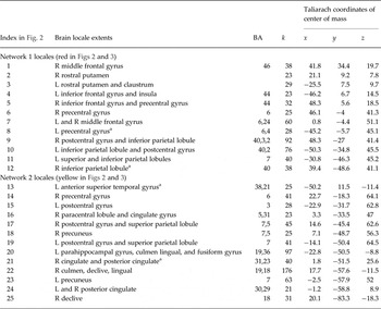
Regions differing in functional connectivity a

BA, Brodmann area; k, number of voxels in cluster; R, right; L, left; ROI, region of interest.
a Contains the ROI identified in the first-stage group analysis. Coordinates differ from the main text when the ROI was enlarged by the second-stage group analysis.
Secondary locale identification
Group differences in global connectivity reflect group differences in connectivity within specific networks (Buckner et al. Reference Buckner, Sepulcre, Talukdar, Krienen, Liu, Hedden, Andrews-Hanna, Sperling and Johnson2009; Gotts et al. Reference Gotts, Simmons, Milbury, Wallace, Cox and Martin2012; Di Martino et al. Reference Di Martino, Yan, Li, Denio, Castellanos, Alaerts, Anderson, Assaf, Bookheimer, Dapretto, Deen, Delmonte, Dinstein, Erti-Wagner, Fair, Gallagher, Kennedy, Keown, Keysers, Lainhart, Lord, Luna, Menon, Minshew, Monk, Mueller, Muller, Nebel, Nigg, O'Hearn, Pelphrey, Peltier, Rudie, Sunaert, Thioux, Tyszka, Uddin, Verhoeven, Wenderoth, Wiggins, Mostofsky and Milham2014). To identify these networks, we followed the procedure established by Gotts et al. (Reference Gotts, Simmons, Milbury, Wallace, Cox and Martin2012). Each of the four primary locales were used as a seed in whole-brain, voxel-wise analyses designed to identify diagnosis differences in iFC between the primary locales and other clusters (‘secondary locales’). These analyses controlled for age category, diagnosis × age category interaction, and nuisance covariates of scanner and motion index (voxel-wise p < 0.001, corrected to p < 0.05 for whole-brain comparisons and number of seeds tested). We combined the secondary locales identified by these analyses with the four primary locales to arrive at a final set of 25 brain locales defined by diagnosis differences in iFC (Table 2).
Locale organization into functional networks
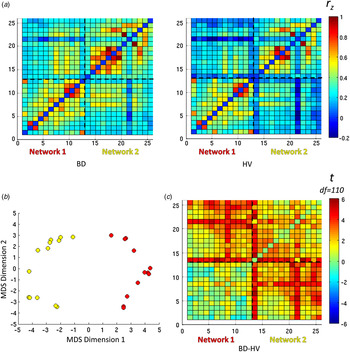
To visualize relationships among locales, a correlation matrix was constructed for each participant and transformed to normally distributed values (Fisher's z), with separate BD and HV group-average matrices calculated after partialling out the effects of age category, diagnosis × age category interaction, scanner, and motion index (Fig. 2a ). These group matrices were then averaged together and submitted to MDS, PCA and k-means cluster analysis in order to identify locales with a similar pattern of correlation with respect to the entire set of locales. All three techniques suggested a two-cluster solution (Fig. 2b ), with an elbow plot indicating that two clusters served as the best tradeoff of variance explained relative to the complexity of the cluster model. These two clusters constituted separate functional networks of locales, and network membership was used to reorder the rows and columns of the correlation matrices (Fig. 2a ) and group t tests (Fig. 2c ) to improve visualization.
(a) Correlation matrices of pairwise brain locale connectivity as Fisher's r to z transform (r z ). Locales are organized in the same order as Table 2, with locale 1 at the bottom left. Dashed lines represent boundaries of networks identified in cluster analyses (b), network 1 = bottom left and network 2 = top right. (b) Locale interrelationships are best described by two networks. Locales are plotted in two-dimensions of Euclidean distance from one another. The dimensions were determined by multidimensional scaling (MDS) all locale to locale interrelationships into two dimensions. The overall pattern suggests two functional networks, best separated by the first dimension. A separate analysis via k-means clustering also suggests a two-network solution, with red markers for locales in network 1 and yellow markers in network 2. (c) Heat map of t-statistics (here, Cohen's d≈t × 0.19) for bipolar disorder–healthy volunteer (BD–HV) contrast of the individual's pairwise r z values controlling for age category (youth v. adult), motion index and scanner. Positive t-statistics, representing hyperconnectivity in BD, are more common amongst pairwise relationships in network 2 and between networks 1 and 2. The threshold for significance is |t| > 3.9 for p < 0.05, Bonferroni corrected for 300 pairwise t tests. df, Degrees of freedom.

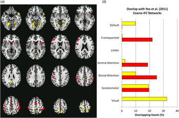
Network 1 (red in Figs 2 and 3) included the bilateral rostral putamen, left insula, right dorsolateral prefrontal cortex, bilateral inferior frontal gyri, sensorimotor areas and inferior parietal lobes. Network 2 (yellow in Figs 2 and 3) comprised temporal and posterior cortical regions (Fig. 3a ; Table 2). Comparison of these functional groupings with the Yeo et al. (Reference Yeo, Krienen, Sepulcre, Sabuncu, Lashkari, Hollinshead, Roffman, Smoller, Zollei, Polimeni, Fischl, Liu and Buckner2011) network parcellation revealed that cortical areas of network 1 mostly overlapped with Yeo and colleagues’ attention, somato-motor and fronto-parietal networks, and cortical areas of network 2 with their visual and somato-motor networks (Fig. 3b ).
(a) Montage of all locales defined by bipolar disorder v. healthy volunteer intrinsic functional connectivity (iFC) differences. Locales clustered into two distinct networks represented by red (network 1) and yellow (network 2). (b) Overlap between the two circuits and seven cortical iFC networks parcellated from 1000 people, reported by Yeo et al. (Reference Yeo, Krienen, Sepulcre, Sabuncu, Lashkari, Hollinshead, Roffman, Smoller, Zollei, Polimeni, Fischl, Liu and Buckner2011).

Differences in the locale interrelationships within and between the identified networks were measured by the standardized mean differences (t scores transformed to Cohen's d) of the BD–HV Fisher r to z (r z ) contrasts accounting for the effects of age category, age category × group interaction, scanner, and motion index (Fig. 2c ). Broadly, in BD v. HV, we found a pattern of hyperconnectivity, i.e. increased positive connectivity, within network 1 [median d = 0.07, interquartile range (IQR) = 0.28; Wilcoxon test V = 1510, p = 0.010], within network 2 (median d = 0.45, IQR = 0.34; V = 1540, p < 0.001] and between networks 1 and 2 (median d = 0.45, IQR = 0.39; V = 16 110, p < 0.001) (Fig. 2c ). The pattern of hyperconnectivity in network 2 and between networks remained after excluding non-euthymic subjects or subjects by class of psychotropic medication (as in Table 1) (p's < 0.05).
With simple partial correlations, we assessed the relationship between the broad pattern of connectivity and mood ratings within the BD group. For each subject, the three types of locale interrelationships, within network 1, within network 2, and between networks, were represented by their median r z . Manic and depressive symptoms did not correlate with subjects’ median r z of locale interrelationships within or between networks, controlling for age category, scanner and motion index (partial r's ranged −0.24 to 0.08, p's > 0.05).
Relationship to nuisance factors
Recent attention has been paid to nuisance factors such as transient head motion in functional connectivity studies (Power et al. Reference Power, Mitra, Laumann, Snyder, Schlaggar and Petersen2014). In the current study, the magnitude of transient motion was included in all group tests as a nuisance covariate, reducing its effect on the group comparisons.
Including scanner as a voxel-wise covariate reduced bias in assessing group or age effects due to differences in signal quality among scanners. Moreover, we tested group differences in amplitude by examining the standard deviation of the signal fluctuations in each locale (Jones et al. Reference Jones, Bandettini, Kenworthy, Case, Milleville, Martin and Birn2010). None of the locales showed between-group differences in amplitude (see online Supplementary Table S3), suggesting that signal quality is not a likely explanation of the group results.
Discussion
Using a data-driven, whole-brain analysis, we identified a pattern of increased global connectivity common to both youth and adults (ages 10–50 years) with BD in four brain regions. Global connectivity at these areas reflected hyperconnectivity within and between a corticostriatal and a temporal-parietal network. Median effect sizes of locale interrelationships were moderate for hyperconnectivity in BD within the second network and between the two networks. Within the first network, the median effect size was small for hyperconnectivity in BD, and many locale interrelationships were similar between the BD and HV groups (Fig. 2c ).
These group differences are consistent with prior findings of whole-brain iFC connectivity studies, particularly in finding widespread dysconnectivity. Both sets of findings suggest that dysfunctional circuitry in BD is broadly distributed and complex (Kupferschmidt & Zakzanis, Reference Kupferschmidt and Zakzanis2011). However, our data do implicate specific regions, such as visual temporal, posterior limbic, paralimbic, parietal, striatal and prefrontal regions, consistent with prior data-driven whole-brain connectivity studies (online Supplementary Table S1). Moreover, the regions we identified are consistent with those found in prior studies of structural and functional abnormalities in BD (Bora et al. Reference Bora, Fornito, Yücel and Pantelis2010; Ellison-Wright & Bullmore, Reference Ellison-Wright and Bullmore2010; Chen et al. Reference Chen, Suckling, Lennox, Ooi and Bullmore2011; Kupferschmidt & Zakzanis, Reference Kupferschmidt and Zakzanis2011). This prior work includes a meta-analysis of structural dysconnectivity (Wise et al. Reference Wise, Radua, Nortje, Cleare, Young and Arnone2016) and a large study documenting structural abnormalities in similar regions in patients with BD I (Fears et al. Reference Fears, Service, Kremeyer, Araya, Araya, Bejarano, Ramirez, Castrillon, Gomez-Franco, Lopez, Montoya, Montoya, Aldana, Teshiba, Abaryan, Al-Sharif, Ericson, Jalbrzikowski, Luykx, Navarro, Tishler, Altshuler, Bartzokis, Escobar, Glahn, Ospina-Duque, Risch, Ruiz-Linares, Thompson, Cantor, Lopez-Jaramilllo, Macava, Molina, Reus, Sabatti, Freimer and Bearden2014). However, these prior studies are based mostly on adults; in our study, iFC abnormalities manifested similarly across age groups. A notable difference between this and prior studies is that we did not detect iFC abnormalities involving the medial prefrontal or anterior limbic areas. However, this could represent type II error. Fronto-limbic iFC abnormalities may be particularly complex and difficult to detect by current iFC methods, as reflected in the inconsistent findings when these regions are directly probed in BD iFC studies (Torrisi et al. Reference Torrisi, Moody, Vizueta, Thomason, Monti, Townsend, Bookheimer and Altshuler2013; Vargas et al. Reference Vargas, López-Jaramillo and Vieta2013) and task-based fMRI studies (Chen et al. Reference Chen, Suckling, Lennox, Ooi and Bullmore2011; Kupferschmidt & Zakzanis, Reference Kupferschmidt and Zakzanis2011).
The first network we identified (red in Figs 2 and 3) includes many brain regions implicated in attention, cognitive control and response processing (Postuma & Dagher, Reference Postuma and Dagher2006; Niendam et al. Reference Niendam, Laird, Ray, Dean, Glahn and Carter2012; Shulman & Corbetta, Reference Shulman, Corbetta and Posner2012). Functional abnormalities in the inferior frontal gyrus and putamen, two regions in this network, have been consistently associated with BD (Chen et al. Reference Chen, Suckling, Lennox, Ooi and Bullmore2011; Kupferschmidt & Zakzanis, Reference Kupferschmidt and Zakzanis2011). Several cognitive deficits in BD, including in response inhibition (Adler et al. Reference Adler, Holland, Schmithorst, Tuchfarber and Strakowski2004; Monks et al. Reference Monks, Thompson, Bullmore, Suckling, Brammer, Williams, Simmons, Giles, Lloyd, Harrison, Seal, Murray, Ferrier, Young and Curtis2004; Leibenluft et al. Reference Leibenluft, Rich, Vinton, Nelson, Fromm, Berghorst, Berghorst, Joshi, Robb, Schachar, Dickstein, McClure and Pine2007; Mazzola-Pomietto et al. Reference Mazzola-Pomietto, Kaladjian, Azorin, Anton and Jeanningros2009; Passarotti et al. Reference Passarotti, Sweeney and Pavuluri2010; Townsend et al. Reference Townsend, Bookheimer, Foland–Ross, Sugar and Altshuler2010) and working memory (Adler et al. Reference Adler, Holland, Schmithorst, Tuchfarber and Strakowski2004; Monks et al. Reference Monks, Thompson, Bullmore, Suckling, Brammer, Williams, Simmons, Giles, Lloyd, Harrison, Seal, Murray, Ferrier, Young and Curtis2004; Townsend et al. Reference Townsend, Bookheimer, Foland–Ross, Sugar and Altshuler2010), are thought to be mediated by dysfunction in these and other regions in this network.
The second network (yellow in Figs 2 and 3) is largely comprised of visual and association areas and their downstream, posterior limbic areas. Of note, compared with the first network, less research in BD focuses on this set of brain regions. Nevertheless, functional abnormalities have been identified in many of the identified brain regions, including the parahipocampal and lingual gyri (Chen et al. Reference Chen, Suckling, Lennox, Ooi and Bullmore2011; Kupferschmidt & Zakzanis, Reference Kupferschmidt and Zakzanis2011). Relative to the first network, it is less clear how disruption in this network is related to impairments in BD, although disruptions in this network are consistent with visuospatial perceptual and encoding impairments in BD (Bora et al. Reference Bora, Yucel and Pantelis2009; Kurtz & Gerraty, Reference Kurtz and Gerraty2009). Specifically, there is evidence in BD of abnormal activation in these regions during fMRI paradigms involving face-emotion processing (Dickstein et al. Reference Dickstein, Rich, Roberson-Nay, Berghorst, Vinton, Pine and Leibenluft2007; Adleman et al. Reference Adleman, Kayser, Olsavsky, Bones, Muhrer, Fromm, Pine, Zarate, Leibenluft and Brotman2013) and during face identity recognition and encoding (Glahn et al. Reference Glahn, Robinson, Tordesillas-Gutierrez, Monkul, Holmes, Green and Bearden2010); the latter may be a BD endophenotype (Fears et al. Reference Fears, Service, Kremeyer, Araya, Araya, Bejarano, Ramirez, Castrillon, Gomez-Franco, Lopez, Montoya, Montoya, Aldana, Teshiba, Abaryan, Al-Sharif, Ericson, Jalbrzikowski, Luykx, Navarro, Tishler, Altshuler, Bartzokis, Escobar, Glahn, Ospina-Duque, Risch, Ruiz-Linares, Thompson, Cantor, Lopez-Jaramilllo, Macava, Molina, Reus, Sabatti, Freimer and Bearden2014; Tseng et al. Reference Tseng, Bones, Kayser, Olsavsky, Fromm, Pine, Leibenluft and Brotman2015).
Our study must be interpreted in light of a number of limitations. First, while we did not detect age-specific abnormalities in iFC in BD, this analysis may have been underpowered to detect age-related differences, with only 17 in the adult group, a wide variation in age, and the difference in age between BD and HV adults. The concern of type II error due to these factors is lessened by lack of a group × age interaction in complementary analyses treating age as a continuous variable (online Supplementary material). Our findings apply primarily to adolescents with BD v. adults and not to young children with BD. Second, data were collected over three scanners. Variance from scanner imbalance may have made it more difficult to detect a group × age interaction. However, because the groups were balanced across scanners, group differences cannot be due to scanner difference. Post-hoc analyses suggest that the pattern of abnormal iFC that we detected is a feature of euthymic BD regardless of medication; however, more research is needed to assess the effects of these potential confounds. Third, due to our sample size, the influence of medication exposure, co-morbid diagnoses and mood state could not be adequately assessed in post-hoc analysis and is an important area for future research.
In conclusion, we found aberrant iFC in BD in two functional networks, one involving corticostriatal areas involved in attention, cognitive control, and response processing, and the other involving parietal and temporal regions associated with late visual and associative processing. Our findings suggest that a number of regions implicated as dysfunctional in BD, based on cognitive and task-based fMRI data, can be organized into two networks that exhibit intrinsic functional hyperconnectivity both within and between them (Robinson et al. Reference Robinson, Thompson, Gallagher, Goswami, Young, Ferrier and Moore2006; Bora et al. Reference Bora, Yucel and Pantelis2009; Kurtz & Gerraty, Reference Kurtz and Gerraty2009). This effort represents an early study in connectome alterations in BD and suggests the importance of future multimodal research to establish the nature of abnormal networks within BD.
Supplementary material
For supplementary material accompanying this paper visit http://dx.doi.org/10.1017/S0033291716000143
Acknowledgements
This research was supported by the Intramural Research Program of the NIMH, and it was conducted under projects ZIA-MH002778 (clinical protocol NCT00006177) and ZIA-MH002786 (clinical protocol NCT00025935).
We would like to thank the participants and families who were involved in this study, and the staff of the Emotion and Development Branch at the NIMH.
Declaration of Interest
C.Z. is listed as a coinventor on a patent for the use of ketamine and its metabolites in major depression. C.Z. has assigned his rights in the patent to the US government but will share a percentage of any royalties that may be received by the government. All other authors have no conflicts of interest or outside financial support to report.