1. Introduction
The purpose of this paper is to shed light on the constraints that the rheological properties of a gravity mass flow (GMF) and the bed over which it flows impose on the formulation of erosion laws in the framework of depth-integrated flow models. Erosion is determined by the flow variables near the bed–flow interface, but this information is not accessible in the type of model we consider. The typical approach – adopted in a large number of depth-averaged models from different fields, as summarized by Eglit & Demidov (Reference Eglit and Demidov2005) – is to postulate a heuristic erosion law with a freely adjustable parameter. On physical grounds, however, the erosion rate must be uniquely determined by the state of the system, hence there must be severe constraints on the allowed form of the erosion law in depth-averaged models.
There exist extensions of depth-averaging that make information on the dynamics of the vertical profiles of the fields available by expanding the fields along the
 $z$
direction in terms of a suitably chosen complete set of basis functions and truncating the series after the first few terms. They are variably termed the method of weighted residuals (Finlayson & Scriven Reference Finlayson and Scriven1966; Kowalski & McElwaine Reference Kowalski and McElwaine2013), Kantorovich technique (Scheiwiller & Hutter Reference Scheiwiller and Hutter1982; Scheiwiller Reference Scheiwiller1986) or long-wave approximation (Ruyer-Quil & Manneville Reference Ruyer-Quil and Manneville2000, Reference Ruyer-Quil and Manneville2002; Scheid, Ruyer-Quil & Manneville Reference Scheid, Ruyer-Quil and Manneville2006). While they hold great promise, we will not pursue them further here because they have not found widespread application yet.
We wish to concentrate on the flow dynamics in this paper and avoid the issue of excess pore pressure, which plays a major role in the process of soil erosion and is discussed, e.g. by Iverson (Reference Iverson2012). This work is mainly theoretical, and for the sake of mathematical tractability we study systems that are not easily realizable in the laboratory. However, the basic principles emerging from our study can be applied to more realistic flow models of different GMF types in the future. Where we attempt to make contact with observations from natural GMFs, we mostly use observations from snow avalanches because their internal dynamics is easier to measure than that of e.g. debris flows or rock avalanches.
1.1. Qualitative information from experiments
The following is a condensed summary of the author’s interpretation of the experimental findings that are most relevant in the present context. Appendix A discusses additional aspects.
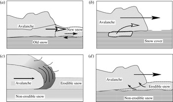
Issler, Gauer & Barbolini (Reference Issler, Gauer, Barbolini and Balean2000) and Gauer & Issler (Reference Gauer and Issler2004) conjectured four different erosion mechanisms in snow avalanches, see figure 1; similar mechanisms are expected to operate in other types of GMFs. With some modifications, they are (i) mechanical ploughing at the front of dense flows, (ii) eruption at the front due to pore-pressure gradients in the bed, (iii) continuous scour along the bed–flow interface, and (iv) intermittent ripping of entire chunks of bed material. There is by now fairly good evidence that these mechanisms indeed operate in snow avalanches, even though the details and the particular conditions of their occurrence have not been fully elucidated yet.
Schematic representation of the four conjectured erosion mechanisms in snow avalanches (modified from Issler et al. Reference Issler, Gauer, Barbolini and Balean2000). Ploughing (a) and eruption (c) occur at the very front of the flow, while intermittent ripping (b) and sustained scour (d) operate along the bottom of the flow. The model presented in this work applies to scour only.

Measurements or direct observations from slush flows are scarce, but one may expect the basic mechanisms to be similar to those in snow avalanches. In debris flows, the measurements of Berger, McArdell & Schlunegger (Reference Berger, McArdell and Schlunegger2011) indicate scour or ripping as the responsible mechanism while ploughing does not seem to play a significant role. Excess pore pressure in the bed facilitates erosion. Hungr & Evans (Reference Hungr and Evans2004) make a strong case for liquefaction of soil by rapid undrained loading to be an important mechanism in strongly entraining rock avalanches, with erosion occurring only after shearing of the substrate has built up sufficient excess pore pressure. The numerical studies by Crosta, Imposimato & Roddeman (Reference Crosta, Imposimato and Roddeman2009a ,Reference Crosta, Imposimato and Roddeman b ) point towards ploughing or scour as the relevant mechanism in rock avalanches, depending on the substrate properties.
Erosion depths of several metres are not uncommon in debris flows, which may last for several minutes or even tens of minutes. The mean erosion speed is then of the order of
 $w_{e}\sim 10^{-3}{-}10^{-2}\ \text{m}\ \text{s}^{-1}$
, but the peak values are likely to be one to two orders of magnitude larger, leading to mass influx rates of up to
 $100{-}1000\ \text{kg}\ \text{m}^{-2}\ \text{s}^{-1}$
. The 1929 Arvel rock avalanche (western Switzerland), whose flow depth probably was close to 50 m, excavated some 20 m of alluvial deposits at the toe of the rock slope in probably less than 10 s, i.e. at an erosion rate of
 $4000\ \text{kg}\ \text{m}^{-2}\ \text{s}^{-1}$
or more.
In dry-snow avalanches, erosion is often limited to the new-snow layer, where the (brittle) shear strength is at most a few kilopascal. For small avalanches, Sovilla, Sommavilla & Tomaselli (Reference Sovilla, Sommavilla and Tomaselli2001) observed entrainment of up to
 $200\ \text{kg}\ \text{m}^{-2}$
and a rapid drop of erosion depth on slopes gentler than approximately 30°. In large dry-snow avalanches, the author has observed erosion depths of 2 m (limited by the amount of erodible snow), corresponding to more than
 $300\ \text{kg}\ \text{m}^{-2}$
, even on counter-slopes. If the entire snow pack is wet and weakened, full-depth erosion and even entrainment of topsoil occur frequently; entrainment may then exceed
 $500\ \text{kg}\ \text{m}^{-2}$
. In these situations, frontal ploughing appears to dominate. Frontal erosion is also important in dry-snow avalanches, though the mechanism may be eruption or ripping rather than ploughing, as interpreted by Sovilla, Burlando & Bartelt (Reference Sovilla, Burlando and Bartelt2006). Those authors report entrainment rates up to
 $350\ \text{kg}\ \text{m}^{-2}\ \text{s}^{-1}$
during short intervals of less than a second. Erosion speeds (rates) sustained over several seconds are, however, usually below
 $0.2\ \text{m}\ \text{s}^{-1}\ (30\ \text{kg}\ \text{m}^{-2}\ \text{s}^{-1})$
at depth-averaged internal avalanche velocities in the range
 $20{-}50\ \text{m}\ \text{s}^{-1}$
.
1.2. Earlier modelling attempts
Despite the low degree of attention entrainment has received in the literature, there have been several attempts to formulate entrainment in a dynamically consistent way. (Depth-resolved formulations including both the bed and the flow do not encounter the conceptual problems that are discussed here, although technical challenges of different nature arise (Crosta et al. Reference Crosta, Imposimato and Roddeman2009a ).) We review them briefly because some show the difficulties we try to overcome in this work, and others deal with different erosion mechanisms that should also be included in a future practical model.
Briukhanov et al. (Reference Briukhanov, Grigorian, Miagkov, Plam, Shurova, Eglit, Yakimov and Ôura1967) and Eglit (Reference Eglit1968) modelled frontal erosion as a shock condition similar to a hydraulic jump and thus circumvented the need for using variables that are lost in depth-averaging. Importantly, the strength of the erodible layer of the bed enters the jump condition for the momentum and so determines the front propagation velocity. The avalanche front is seen as a non-material boundary that moves faster than the particles in the flow and that extends through the entire erodible snow layer, whose depth has to be specified a priori. Experimental observations show, however, that in many cases only part of the new-snow layer, which typically can be considered the erodible layer, is entrained by the flow. We expect this entrainment theory to be particularly pertinent for wet-snow avalanches, but very little work has been done on this topic to date.
One of the very few proposals for determining the erosion rate in a dynamically consistent way without adjustable parameters is due to Grigorian & Ostroumov (Reference Grigorian and Ostroumov1977), later adapted by Sovilla et al. (Reference Sovilla, Burlando and Bartelt2006). As in Eglit’s model, they treat the interface between the bed and the flow as a shock front, but let it be inclined at a variable angle
 ${\it\alpha}$
so that the model describes scour rather than ploughing and the erosion depth is not determined a priori. Mass and momentum balance across the shock front determine
 ${\it\alpha}$
as a function of the overburden pressure, the velocity, and the strength of the snow cover; the erosion speed,
 $w_{e}$
, is then given in terms of the depth-averaged flow velocity,
 ${\bar{u}}$
, by
 $w_{e}={\bar{u}}\tan {\it\alpha}$
. A debatable point, however, is their adding the stagnation pressure of the flow to the hydrostatic overburden pressure.
Cherepanov & Esparragoza (Reference Cherepanov and Esparragoza2008) adopted a fracture-mechanical approach, emphasizing the energy expended in breaking the bonds of the snow particles in the bed. In this way, they arrived at a natural description of ripping while scour does not appear to arise naturally. Focusing on the fracture-mechanical aspects of the problem, they did not deal with the flow dynamics near the interface. Their approach is in many aspects complementary to ours, but it is not obvious at this point how to combine them. We will not deal with ripping in this paper, but comment on its connection to the inherent limits of applicability of the model to be developed here.
The earliest attempt known to the author that emphasizes the role of the flow rheology is the erosion formula by Norem & Schieldrop (Reference Norem and Schieldrop1991) for a frictional-visco-plastic fluid of density
 ${\it\rho}$
, flow depth
 $h$
and depth-averaged velocity
 ${\bar{u}}$
on a slope inclined at an angle
 ${\it\theta}$
. As it showcases all the difficulties encountered in the quest for a truly consistent solution of the problem, we briefly discuss it here. They considered the case where the bed shear strength,
 ${\it\tau}_{c}$
, is smaller than the shear stress at the bottom of the flow,
 ${\it\sigma}_{xz}^{(b)}$
; the latter depends on
 $h$
and the shear rate immediately above the bed,
 $\dot{{\it\gamma}}_{b}$
. They approximate
 $\dot{{\it\gamma}}_{b}$
from the depth-averaged velocity,
 ${\bar{u}}$
, and the chosen rheology by assuming the velocity profile shape of a non-eroding flow at equilibrium. A momentum flux
 ${\it\rho}w_{e}{\bar{u}}$
from the flow to the eroded material is required to accelerate the latter. Matching this momentum flux to the (fictitious) discontinuity of the shear stress at the interface,
 ${\it\sigma}_{xz}^{(b)}-{\it\tau}_{c}$
, the entrainment rate is found to be
 $$\begin{eqnarray}{\it\rho}w_{e}=\frac{{\it\sigma}_{xz}^{(b)}(h,{\bar{u}})-{\it\tau}_{c}}{{\bar{u}}}.\end{eqnarray}$$
The gravitational traction on the flow along the slope being
 ${\it\sigma}_{g}\equiv {\it\rho}hg\sin {\it\theta}$
, the acceleration of the flow becomes
 $({\it\tau}_{g}-{\it\sigma}_{xz}^{(b)})/({\it\rho}h)$
with these assumptions. Norem & Schieldrop’s model considers only one-directional coupling between the erosion process and the flow: it disregards the modification of the velocity profile by the entrainment process, i.e. the details of how the eroded material is incorporated into the flow. This may lead to significant errors in determining the evolution of both the velocity and the erosion rate. Iverson (Reference Iverson2012) encountered the same dilemma and discussed different possible assumptions, but elementary arguments do not suffice to select the correct solution or at least the best approximation.
In a number of laboratory set-ups for granular-flow experiments, e.g. rotating-drum or sand-pile experiments, entrainment is an essential part of the process and has therefore been studied by several authors. An erodible bed increases the mobility of dry granular flows substantially according to the laboratory experiments by Mangeney et al. (Reference Mangeney, Roche, Hungr, Mangold, Faccanoni and Lucas2010). Bouchaud et al. (Reference Bouchaud, Cates, Ravi Prakash and Edwards1994) proposed the influential BCRE model for the evolution of sand piles (assuming thin flows), which was later modified for thick flows by Boutreux, Raphaël & de Gennes (Reference Boutreux, Raphaël and de Gennes1998). Conversion of static grains into rolling ones and vice-versa, i.e. entrainment and deposition, is the essential ingredient in the model. It emphasizes the notion of an equilibrium slope and the role of curvature, with hollows being filled in and ridges being eroded preferentially, while it does not consider the rheology of the flowing material explicitly. Neither does the flow velocity enter the expression for the erosion rate explicitly, but it may influence it through two parameters whose values are not determined by the BCRE theory. As very lucidly reviewed by Douady, Andreotti & Daerr (Reference Douady, Andreotti and Daerr1999), Aradian, Raphaël & de Gennes (Reference Aradian, Raphaël and de Gennes2002) were able to remedy this shortcoming by formulating the problem as a depth-averaged flow model and assuming Coulomb friction and a linear velocity profile. The latter is suggested by experiments on very dense gravity-driven shear flows in a vertical plane, which find the shear rate to be determined by the gravitational acceleration
 $g$
and the particle diameter
 $d$
as
 $\dot{{\it\Gamma}}_{0}\sim \sqrt{g/d}$
irrespective of the vertical position inside the flow (see e.g. Rajchenbach Reference Rajchenbach2003 for a brief review and a theoretical analysis). The resulting model has the same structure as the BCRE model, but the coefficients in the expression for the erosion rate are now fixed. In our notation, their result reads
 $$\begin{eqnarray}w_{e}=\frac{g(\sin {\it\theta}-{\it\mu}\cos {\it\theta})}{\dot{{\it\Gamma}}_{0}}=\frac{2gh(\sin {\it\theta}-{\it\mu}\cos {\it\theta})}{{\bar{u}}}.\end{eqnarray}$$
The stumbling block in the Norem–Schieldrop model is avoided here because this rheology allows essentially only one shear rate, irrespective of whether erosion takes place or not. In a rotating drum, on the other hand, the rotation speed determines the erosion rate, but the shapes of the interfaces and the avalanche surface as well as the flow velocity are unknown. In his elegant theoretical and experimental study, Gray (Reference Gray2001) obtained explicit solutions assuming slip conditions and a uniform velocity profile.
Experiments on a snow chute have revealed piece-wise linear velocity profiles, with high shear very near the bed and significantly less shear above (Bouchet et al. Reference Bouchet, Naaim, Bellot and Ousset2004). This led Naaim et al. (Reference Naaim, Naaim-Bouvet, Faug and Bouchet2004) to adapting the approach by Douady et al. (Reference Douady, Andreotti and Daerr1999) to a snow-avalanche model that can be applied to practical problems. Important achievements of that work are conceptually separating the erosion process from the entrainment process, showing explicitly how the eroded material is entrained into the flow, and emphasizing the crucial role of the shear rate near the bed. Within the assumptions made, they obtain a consistent and uniquely determined solution, but it is an open question to what degree the piece-wise linear velocity profile is able to describe natural avalanches.
1.3. Simplifications and limitations
Among the four erosional mechanisms mentioned in § 1.1, we focus exclusively on modelling scour in this paper. For a realistic description of the motion of snow avalanches, models for ripping and frontal erosion need to be developed as well, however.
In the following, we will consider two example rheological laws, namely a Bingham fluid and a frictional–collisional (FC) granular fluid. The relation between the shear rate and the shear stress for plane-shear flows can be written as
 $$\begin{eqnarray}\hat{{\it\sigma}}_{xz}=\text{sgn}(\dot{{\it\gamma}})(\hat{{\it\tau}}_{y}+{\it\nu}|\dot{{\it\gamma}}|)\end{eqnarray}$$
for the Bingham fluid, with
 $\hat{{\it\tau}}_{y}$
the yield strength and
 ${\it\nu}$
the (Bingham) viscosity, and
 $$\begin{eqnarray}\hat{{\it\sigma}}_{xz}=\text{sgn}(\dot{{\it\gamma}})({\it\mu}\hat{{\it\sigma}}_{zz}+K\dot{{\it\gamma}}^{2})\end{eqnarray}$$
for the FC granular fluid. Here and henceforth, stresses with a caret
 $(\,\hat{\ }\,)$
are stresses divided by the flow density, e.g.
 $\hat{{\it\tau}}_{y}\equiv {\it\tau}_{y}/{\it\rho}_{f}$
; in our notation, compressive stresses are positive. Also,
 ${\it\mu}$
is the Coulomb friction coefficient and
 $K$
(units
 $\text{m}^{2}$
) the consistency. Both rheological laws exhibit threshold behaviour: if the shear stress is less than
 $\hat{{\it\tau}}_{y}$
and
 ${\it\mu}\hat{{\it\sigma}}_{zz}$
, respectively, the material does not flow and the shear stress cannot be computed directly from the rheological equation.
The main reason for choosing these two example rheological equations is their mathematical tractability. However, there are also a number of flow models in practical use that apply them: the Bingham rheology quite successfully models clay-rich mudflows and subaqueous debris flows (Hungr Reference Hungr1995; Imran, Harff & Parker Reference Imran, Harff and Parker2001; Pastor et al.
Reference Pastor, Haddad, Sorbino, Cuomo and Drempetic2009); it may also be applicable to wet-snow avalanches, but few measurements exist and little work has been done on this problem. The FC rheology is a candidate rheology for describing dry-snow avalanches and rock avalanches. It can be considered a simplified version of the NIS model (Norem, Irgens & Schieldrop Reference Norem, Irgens, Schieldrop, Salm and Gubler1987) or a minimal extension of the Voellmy (Reference Voellmy1955) friction law to a complete rheological model – two models widely used in snow avalanche engineering. It also duplicates some features of rheological laws based on the kinetic theory of granular media (see e.g. Louge Reference Louge2003) like the depth-averaged velocity growing with the flow height as
 ${\bar{u}}\propto h^{3/2}$
. However, it does not predict the existence of a minimal flow height,
 $h_{stop}$
, or the concavity of the steady-state velocity profile at the base.
In the interplay between the flow rheology and the entrainment rate, the stress boundary condition at the interface between bed and flow plays a key role, as will be seen in §§ 2.1 and 2.2. We make the simplest assumption, namely that the bed material is a perfectly brittle solid that breaks instantaneously when the shear stress reaches a critical value,
 ${\it\tau}_{c}$
. We postulate that the shear stress does infinitesimal work breaking the surface of the bed and that the eroded material assumes the rheological properties of the flow. While obviously an idealization, these assumptions are not too far from reality in the case of natural snow, which becomes brittle at shear rates above approximately
 $10^{-3}\ \text{s}^{-1}$
and breaks as soon as the shear reaches values of the order of
 $10^{-2}$
. Mellor (Reference Mellor1977, pp. 31–32) indicates that existing measurements of the comminution energy per unit volume of snow differ by orders of magnitude, but even the highest values appear to be in the range of the frictional work expended by the flowing avalanche. Erosion is the result of friction between the flowing particles and the bed, and it appears reasonable to suppose that scouring is a rather efficient erosion mechanism. Thus there is no indication that our assumptions are in disagreement with the properties of snow, but the question deserves further study.
The postulated brittleness of the bed suggests that the boundary condition for the shear stress at the bed–flow interface should be
 $$\begin{eqnarray}{\it\sigma}_{xz}^{(b)}\equiv {\it\sigma}_{xz}|_{z=0}={\it\tau}_{c}.\end{eqnarray}$$
(For simplicity, throughout this paper we restrict ourselves to flows in the vertical plane, with the
 $x$
direction along the slope and
 $z$
perpendicular to it.) This is analogous to Owen’s (Reference Owen1964) hypothesis for the bed shear stress in aeolian sand or snow transport. We cannot rigorously prove the validity of (1.5), but there is a negative feed-back mechanism that makes it plausible: if the slope is steep enough and the flow sufficiently thick for erosion to be possible, erosion would nevertheless stop if
 ${\it\sigma}_{xz}^{(b)}$
were to fall below
 ${\it\tau}_{c}$
. The flow would then accelerate and
 ${\it\sigma}_{xz}^{(b)}$
would grow again until the threshold is reached and erosion resumes. If the bed shear stress exceeds the threshold, the shear stress inside a finite layer at the top of the bed will be larger than
 ${\it\tau}_{c}$
and instantaneous failure will occur throughout a finite-depth layer. While this mass is being accelerated,
 ${\it\sigma}_{xz}^{(b)}$
at the newly formed interface drops below
 ${\it\tau}_{c}$
and the system is being driven back to the equilibrium shear stress (1.5).
The adequacy of the brittleness assumption for other types of GMFs is debatable. Taking rock avalanches as an example, the brittleness assumption is a poor approximation for a talus slope or clayey soil; indeed, Hungr & Evans (Reference Hungr and Evans2004) present strong evidence for massive entrainment of liquefied soil to form a lubricating layer and to increase the run-out distance of rock avalanches dramatically. Weathered bedrock, however, may show behaviour similar to the one we postulate. In the case of a Bingham fluid, the assumption of a perfectly brittle bed turning into a yield stress fluid upon entrainment appears counter-intuitive. Nevertheless, it may still be an acceptable first approximation if the bed material weakens rapidly after its peak strength has been reached. The bed undergoes some shearing and erosion is not immediate, but these effects may be negligible on the time and length scales of the flow. In quick-clay, such remoulding will cause the yield strength and viscosity of the material to drop by orders of magnitude, but not to zero. The erosion process is no longer localized at an interface of infinitesimal thickness in such materials, but occurs gradually across a layer. However, if this layer is sufficiently thin, the brittleness assumption should be a convenient starting point for a more detailed analysis.
The assumption of a constant shear strength
 ${\it\tau}_{c}$
throughout the bed immediately leads to a geotechnical stability problem: the shear stress in an inclined bed increases with depth due to the material’s own weight. Thus, if the shear stress equals
 ${\it\tau}_{c}$
at the top of the bed when erosion occurs, it exceeds
 ${\it\tau}_{c}$
deeper in the bed. The only way to circumvent instantaneous collapse of the bed throughout its entire depth is to assume that
 ${\it\tau}_{c}$
increases with depth more rapidly than the gravitational traction, i.e.
 $$\begin{eqnarray}\text{d}{\it\tau}_{c}/\text{d}z<-{\it\rho}_{b}g\sin {\it\theta},\end{eqnarray}$$
where
 ${\it\rho}_{b}$
is the bed density,
 $g$
the gravitational constant, and
 ${\it\theta}$
the slope angle. Such behaviour is not unrealistic; for example, it may be due to sintering or cementing in cohesive materials like snow or clay. For simplicity, we assume here that the bed is geotechnically stable even under continuous erosion at its surface, where its shear strength is postulated to be constant.
We will not discuss deposition in this paper (except for a few remarks in § 2.1). In non-cohesive granular materials, particles are equally rapidly trapped by a hollow as they are dislodged by sufficiently energetic collisions. Hence deposition can be treated in the same way as erosion in those systems. However, there are fundamental differences between the two processes for the cohesive solid beds we consider. The forces mediating the bonds between particles have very short range. The complex processes forging bonds therefore require intimate contact and typically operate on time scales of seconds or longer. In contrast, bonds break in the course of microseconds or less under the prevalent conditions in a rapid GMF. As discussed by Issler & Jóhannesson (Reference Issler and Jóhannesson2011), deposition is also contingent upon the bed exerting a larger shear stress on the flow than the latter can sustain internally; if this condition is not fulfilled, the flow is simply decelerated. Experiments with piles of cohesionless granular materials show the neutral angle,
 ${\it\phi}_{n}$
, for which trapping of rolling grains is equally probable as dislodging of static grains, to be somewhat larger than the dynamic friction angle,
 ${\it\phi}_{d}$
, so that true deposition may occur in that case. Flows of settling particle suspensions provide another example where the condition is met and deposition is observed: in the transition layer between the bed and the flow, particles come into frictional contact with each other and the shear stress may greatly exceed the viscous shear stress inside the flow. However, such effects are unlikely to occur in the type of idealized solid/fluid material we consider.
The present work originated from the investigation of a model that is simplified with respect to both rheology and flow configuration to the point where explicit solutions can be obtained (Issler & Jóhannesson Reference Issler and Jóhannesson2006, Reference Issler and Jóhannesson2011). These solutions are invaluable for understanding the basic principles at work and for finding ways of tackling the full problem, either numerically or through analytic approximations. The model will therefore be discussed first in § 2.1. Section 2.2 shows that solutions can also be found at least for one nonlinear rheology of interest in the context of granular flows. At the present stage of experiments on GMFs, it is difficult to test our theoretical predictions in detail, but available measurements from snow avalanches show that they have the correct order of magnitude.
Extending the theory to variable flow depth is challenging mathematically. Issler & Pastor Pérez (Reference Issler and Pastor Pérez2011) and Eglit & Yakubenko (Reference Eglit and Yakubenko2014) therefore applied numerical methods in a depth-resolved framework, but retained the uniform-flow approximation so that derivatives in the flow direction vanish. Those studies provided clues for developing approximate, but dynamically self-consistent expressions for the erosion speed (§ 3). Closer examination of these formulae reveals that their range of applicability is limited in terms of admissible flow depths and velocities. We do not yet have a full solution over the entire range of these variables, but the physical reason behind the breakdown of our method emerges in § 4 and indicates promising directions for future work on the topic.
2. Consistent erosion models for quasi-stationary flows
This section aims at elucidating the interplay between the flow rheology and the boundary condition for the shear stress in detail. We simplify the problem in another respect, however, by considering a quasi-stationary but eroding flow. As pointed out by Iverson (Reference Iverson2012), such a flow cannot exist in reality, but we can create it as a thought experiment by assuming the slope and the flow to be infinitely long. Erosion moves the interface between the bed and the flow at a speed
 $-w_{e}$
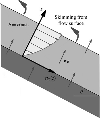
in the direction normal to the bed. In order to keep the flow depth constant, mass is skimmed from the top of the flow at the same rate as it is eroded from the bed, without exerting any force on the flow, see figure 2. For simplicity, we assume the densities of the snow cover and the avalanche to be equal and use a coordinate system moving with the interface.
Sketch of the thought experiment representing the flow configuration studied in § 2. The slope and the flow are infinitely long. The bed is eroded at the speed
 $w_{e}$
. We use a moving coordinate system with
 $z=0$
at the bed–flow interface; thus the bed and flow have a uniform bed-normal upward velocity
 $w_{e}$
. Without disturbing the flow, mass is skimmed off the top surface (curved arrows) at the same rate as it is eroded from the bed.

In this set-up, with
 $x$
along the flow direction and
 $z$
normal to the bed, the velocity field reduces to
 $$\begin{eqnarray}\boldsymbol{u}(x,y,z,t)=(u(z),0,0)\end{eqnarray}$$
and explicitly satisfies the mass balance equation
 $\boldsymbol{{\rm\nabla}}\boldsymbol{\cdot }\boldsymbol{u}=0$
. The momentum balance equation is trivially satisfied in the
 $y$
direction and provides the expression for hydrostatic pressure in the
 $z$
direction:
 $\hat{{\it\sigma}}_{zz}(z)=-g_{z}\,(h-z)$
, where
 $g_{z}=-g\cos {\it\theta}$
,
 $g$
is the gravitational acceleration and
 ${\it\theta}$
the slope angle. (Here and in the rest of the paper, we designate specific stresses and material strengths, i.e. stresses and strengths divided by the flow density, by a caret over the symbol. We use
 $\hat{{\it\sigma}}_{ij}$
for the specific stresses and
 $\hat{{\it\tau}}_{c}$
,
 $\hat{{\it\tau}}_{y}$
for specific strengths.) In the
 $x$
direction, this equation describes the acceleration of the eroded material from speed zero at the interface
 $z=0$
to
 $u(h)$
at
 $z=h$
under the action of gravity (with
 $g_{x}=g\sin {\it\theta}$
) and the shear stress gradient inside the avalanche:
 $$\begin{eqnarray}w_{e}\dot{{\it\gamma}}(z)=g_{x}+\hat{{\it\sigma}}_{xz}^{\prime }(z),\end{eqnarray}$$
with the prime here and henceforth denoting an ordinary derivative with respect to
 $z$
when there is no dependence on other variables. The left-hand side is the convective derivative in our simplified setting, and the right-hand side contains the body force and the external forces on an infinitesimal control volume at a distance
 $z$
from the interface. Note that (2.2) reduces to (1.2) if one assumes
 $\dot{{\it\gamma}}(z)=\dot{{\it\Gamma}}_{0}$
and the Coulomb friction law
 $\hat{{\it\sigma}}_{xz}(z)=-{\it\mu}(h-z)g_{z}$
.
Let the rheological relation between the shear rate and the shear stress be of the form
 $$\begin{eqnarray}\hat{{\it\sigma}}_{xz}(z)=\hat{{\it\sigma}}_{xz}(\dot{{\it\gamma}}(z),\hat{{\it\sigma}}_{zz}(z)).\end{eqnarray}$$
The shear stress gradient is then given by
 $$\begin{eqnarray}\frac{\text{d}\hat{{\it\sigma}}_{xz}}{\text{d}z}(z)=\frac{\partial \hat{{\it\sigma}}_{xz}}{\partial \dot{{\it\gamma}}}(z)\,\dot{{\it\gamma}}^{\prime }(z)+\frac{\partial \hat{{\it\sigma}}_{xz}}{\partial \hat{{\it\sigma}}_{zz}}(z)\,\hat{{\it\sigma}}_{zz}^{\prime }(z).\end{eqnarray}$$
Inserting this into (2.2), one obtains an ordinary (but in general nonlinear) differential equation for the shear rate
 $\dot{{\it\gamma}}(z)$
. The erosion speed,
 $w_{e}$
, plays the role of a parameter, but it can be determined by imposing the boundary condition
 $\hat{{\it\sigma}}_{xz}(0)=\hat{{\it\tau}}_{c}$
.
2.1. Eroding Bingham fluid
In the absence of entrainment, a two-dimensional, stationary, gravity-driven simple shear flow of a Bingham fluid exhibits a plug layer that extends from the surface of the flow at
 $z=h$
to a height
 $z=r$
above the bed:
 $$\begin{eqnarray}r=h-\frac{\hat{{\it\tau}}_{y}}{g_{x}}.\end{eqnarray}$$
The shear stress profile is linear,
 $$\begin{eqnarray}\hat{{\it\sigma}}_{xz}^{(0)}(z)=g_{x}(h-z),\end{eqnarray}$$
the shear rate diminishes linearly from the bed to the height
 $r$
,
 $$\begin{eqnarray}\dot{{\it\gamma}}^{(0)}(z)=\left\{\begin{array}{@{}ll@{}}\displaystyle \frac{g_{x}(r-z)}{{\it\nu}},\quad & z\leqslant r,\\ 0,\quad & z\geqslant r,\end{array}\right.\end{eqnarray}$$
and the velocity profile is parabolic in the shear layer if there is no sliding at the bed,
 $$\begin{eqnarray}u^{(0)}(z)=\left\{\begin{array}{@{}ll@{}}\displaystyle \frac{g_{x}}{2{\it\nu}}(2rz-z^{2}),\quad & z\leqslant r,\\ \displaystyle \frac{g_{x}}{2{\it\nu}}r^{2},\quad & z\geqslant r.\end{array}\right.\end{eqnarray}$$
With entrainment, the velocity profile will remain constant in time in our idealized situation, but deviate from (2.8). The shear stress being zero at the surface
 $z=h$
, there will still be a plug layer. As there is no acceleration, the plug layer depth is unchanged from the expression (2.5). Upon applying (2.4) and (1.3) for a Bingham fluid to (2.2), we obtain
 $$\begin{eqnarray}\dot{{\it\gamma}}^{\prime }(z)-\frac{w_{e}}{{\it\nu}}\,\dot{{\it\gamma}}(z)=-\frac{g_{x}}{{\it\nu}},\quad 0\leqslant z\leqslant r.\end{eqnarray}$$
Temporarily assuming the entrainment speed
 $w_{e}$
to be given and applying the boundary condition
 $\dot{{\it\gamma}}(r)=0$
, we find the solution
 $$\begin{eqnarray}\dot{{\it\gamma}}(z)=\left\{\begin{array}{@{}ll@{}}\displaystyle \frac{g_{x}}{w_{e}}(1-\text{exp}[-(w_{e}/{\it\nu})(r-z)]),\quad & 0\leqslant z\leqslant r,\\ 0\quad & r\leqslant z\leqslant h.\end{array}\right.\end{eqnarray}$$
From this we obtain the following velocity and shear-stress profiles if we assume no slip at the bed:
 $$\begin{eqnarray}\displaystyle & \displaystyle u(z)=\left\{\begin{array}{@{}ll@{}}\displaystyle \frac{g_{x}}{w_{e}}\left[z-\frac{{\it\nu}}{w_{e}}(\text{exp}[-(w_{e}/{\it\nu})(r-z)]-\text{exp}[-(w_{e}/{\it\nu})r])\right],\quad & 0\leqslant z\leqslant r,\\ \displaystyle \frac{g_{x}}{w_{e}}\left[r-\frac{{\it\nu}}{w_{e}}(1-\text{exp}[-(w_{e}/{\it\nu})r])\right],\quad & r\leqslant z\leqslant h,\end{array}\right. & \displaystyle\end{eqnarray}$$
 $$\begin{eqnarray}\displaystyle & \displaystyle \hat{{\it\sigma}}_{xz}(z)=\left\{\begin{array}{@{}ll@{}}\displaystyle \hat{{\it\tau}}_{y}+\frac{{\it\nu}g_{x}}{w_{e}}(1-\text{exp}[-(w_{e}/{\it\nu})(r-z)]),\quad & 0\leqslant z\leqslant r,\\ g_{x}(h-z),\quad & r\leqslant z\leqslant h.\end{array}\right. & \displaystyle\end{eqnarray}$$
 $w_{e}\rightarrow 0$
.
These formulae suggest the following scaling for lengths, velocities and stresses, with dimensionless quantities designated by a tilde:
 $$\begin{eqnarray}\left.\begin{array}{@{}l@{}}\displaystyle z=h\tilde{z},\quad \hat{{\it\sigma}}_{xz}=g_{x}h\tilde{{\it\sigma}}_{xz},\quad \hat{{\it\tau}}_{y}=g_{x}h\tilde{{\it\tau}}_{y},\quad \hat{{\it\tau}}_{c}=g_{x}h\tilde{{\it\tau}}_{c},\\ \displaystyle r=h\tilde{r},\quad u=\frac{g_{x}h^{2}}{2{\it\nu}}{\tilde{u}}_{x},\quad w_{e}=\frac{{\it\nu}}{h}\tilde{w}_{e};\end{array}\right\}\end{eqnarray}$$
note that
 $\tilde{r}=1-\tilde{{\it\tau}}_{y}$
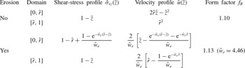
. Then the velocity and stress profiles and the momentum form factor (or Boussinesq coefficient), defined by
 $$\begin{eqnarray}f_{B}=\frac{\overline{u^{2}}}{{\bar{u}}^{2}}=\frac{\displaystyle h\int _{0}^{h}u^{2}(z)\text{d}z}{\displaystyle \left[\int _{0}^{h}u(z)\text{d}z\right]^{2}},\end{eqnarray}$$
are given by the expressions listed in table 1.
Vertical profiles of shear stress and longitudinal velocity in steady-state flows of Bingham fluids with and without entrainment. All quantities are non-dimensionalized according to (2.13). In the limit of vanishing entrainment, i.e.
 $\tilde{w}_{e}\rightarrow 0$
, all profiles with entrainment reduce to the corresponding profiles without entrainment. The Boussinesq form factor
 $f_{B}$
given by (2.14) is evaluated for
 $\tilde{r}=0.5$
, and for
 $\tilde{{\it\tau}}_{c}=0.7$
in the case of entrainment. The value of
 $\tilde{w}_{e}$
indicated in brackets corresponds to the physically consistent entrainment rate.

It remains to implement the stress boundary condition
 $\hat{{\it\sigma}}_{xz}(0)=\hat{{\it\tau}}_{c}$
or
 $\tilde{{\it\sigma}}_{xz}(0)=\tilde{{\it\tau}}_{c}$
. Using the pertinent expression from table 1 at
 $\tilde{z}=0$
yields the transcendental equation
 $$\begin{eqnarray}\frac{1}{\tilde{w}_{e}}(1-\text{exp}[-(1-\tilde{{\it\tau}}_{y})\tilde{w}_{e}])=\tilde{{\it\tau}}_{c}-\tilde{{\it\tau}}_{y}\end{eqnarray}$$
for the dimensionless erosion rate
 $\tilde{w}_{e}$
in terms of the dimensionless yield strength
 $\tilde{{\it\tau}}_{y}$
and the dimensionless shear strength of the snow cover,
 $\tilde{{\it\tau}}_{c}$
. Note the physical requirement
 $0\leqslant \tilde{{\it\tau}}_{y}<\tilde{{\it\tau}}_{c}<1$
. Equation (2.15) can be recast as
 $$\begin{eqnarray}w\text{e}^{w}=v\text{e}^{v},\end{eqnarray}$$
where
 $$\begin{eqnarray}v:=-\frac{1-\tilde{{\it\tau}}_{y}}{\tilde{{\it\tau}}_{c}-\tilde{{\it\tau}}_{y}},\quad w=v+(1-\tilde{{\it\tau}}_{y})\tilde{w}_{e}.\end{eqnarray}$$
Here,
 $v$
takes values in the range
 $-\infty <v<-1$
so that
 $v\text{e}^{v}\in D:= ]-1/\text{e},0[$
. The general solution can be expressed in terms of Lambert’s non-elementary
 $W$
function, which is defined as the solution
 $x(y)$
of the equation
 $x\text{e}^{x}=y$
. In the possible range of
 $v$
,
 $W$
is two-valued, with
 $W_{0}(-1/\text{e})=W_{-1}(-1/\text{e})=-1$
and
 $W_{0}(D)=\, ]-1,0[$
,
 $W_{-1}(D)= ]-\infty ,-1[$
. The equation for the dimensionless erosion speed now reads
 $w=W(v\text{e}^{v})$
. As
 $v<w$
,
 $v$
corresponds to the lower branch
 $W_{-1}$
and
 $w=W_{0}(v\text{e}^{v})$
. The erosion speed thus becomes
 $$\begin{eqnarray}w_{e}=\frac{{\it\nu}}{h}\,\frac{1}{1-\tilde{{\it\tau}}_{y}}[W_{0}(v\text{e}^{v})-v];\end{eqnarray}$$
the dimensionless quantity
 $\tilde{w}_{e}$
is plotted as a function of
 $\tilde{{\it\tau}}_{y}$
and
 $\tilde{{\it\tau}}_{c}$
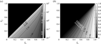
in figure 3(a). As figure 3(b) shows, favourable conditions for entrainment lead to low flow velocities.
Quasi-stationary flow of a Bingham fluid with non-dimensional yield strength
 $\tilde{{\it\tau}}_{y}$
over an erodible bed with dimensionless shear strength
 $\tilde{{\it\tau}}_{c}$
: (a) dimensionless entrainment rate
 $\tilde{w}_{e}$
and (b) ratio of surface velocities of entraining and non-entraining flows. Quasi-stationary eroding flow is not possible for
 $\tilde{{\it\tau}}_{y}>\tilde{{\it\tau}}_{c}$
.

One may obtain a first-order approximation and circumvent the evaluation of the nonlinear equation (2.15) by using the parabolic shape of the velocity profiles of non-entraining flows even with entrainment or deposition. To this end, apply the boundary condition for the bed shear stress to the integrated form of (2.2) to get
 $w_{e}u(h)=hg_{x}-\hat{{\it\tau}}_{c}$
, and to (1.3). Together with the relation
 $u(h)=u(r)=2r\dot{{\it\gamma}}(0)$
for a parabolic velocity profile, one arrives at
 $$\begin{eqnarray}\displaystyle & \displaystyle \tilde{w}_{e}\approx \frac{2}{\tilde{{\it\tau}}_{c}-\tilde{{\it\tau}}_{y}}\,\frac{1-\tilde{{\it\tau}}_{c}}{1-\tilde{{\it\tau}}_{y}}, & \displaystyle\end{eqnarray}$$
 $$\begin{eqnarray}\displaystyle & {\tilde{u}}(1)\approx (1-\tilde{{\it\tau}}_{y})(\tilde{{\it\tau}}_{c}-\tilde{{\it\tau}}_{y}). & \displaystyle\end{eqnarray}$$
 $({\it\tau}_{c}-{\it\tau}_{y})/(hg_{x})$
. In the case
 $\tilde{{\it\tau}}_{c}=0.7$
,
 $\tilde{{\it\tau}}_{y}=0.5$
(implying
 $\tilde{r}=0.5$
), the approximation yields
 $\tilde{w}_{e}=6.0$
and
 ${\tilde{u}}(1)=0.1$
, whereas the self-consistent solution is
 $\tilde{w}_{e}=4.46$
and
 ${\tilde{u}}(1)=0.134$
.
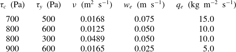
Comparison of the predicted entrainment rates with experimental data is difficult because erosion rates have rarely been measured, and then mostly in dry-snow avalanches (Gauer & Issler Reference Gauer and Issler2004; Sovilla Reference Sovilla2004) for which a Bingham fluid is a poor approximation. For an order-of-magnitude check, table 2 lists entrainment speeds and rates that would result from a typical slow, humid granular snow avalanche on a 30° slope, with a flow depth of 1 m, a density of
 $200\ \text{kg}\ \text{m}^{-3}$
and a surface velocity of
 $20\ \text{m}\ \text{s}^{-1}$
. The values of
 ${\it\tau}_{c}$
were chosen in a realistic range while
 ${\it\tau}_{y}$
and
 ${\it\nu}$
result from the requirement
 $u(h)=20\ \text{m}\ \text{s}^{-1}$
.
Examples of entrainment rates obtained for different combinations of snow-cover strength (
 ${\it\tau}_{c}$
), yield strength (
 ${\it\tau}_{y}$
) and Bingham viscosity (
 ${\it\nu}$
) in the flow. Idealized stationary flow with density
 $200\ \text{kg}\ \text{m}^{-3}$
, flow height 1 m and surface velocity
 $20\ \text{m}\ \text{s}^{-1}$
on a 30° slope.

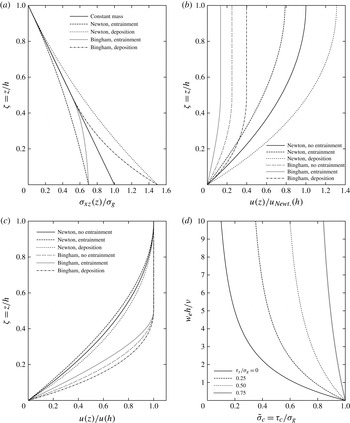
To conclude this section and illustrate the similarities and differences between deposition and entrainment, we modify our model, supplying material at the top at surface velocity and removing it at the bottom after it has come to rest. Deposition makes the non-dimensionalized shear stress profile (cf. figure 4
a) convex instead of concave in the shear layer; the value at the bed interface exceeds the gravitational traction. Similarly, the velocity normalized by its value at the surface is larger in the shear layer than in the flow without deposition, opposite to the effect of entrainment (see figure 4
c). In contrast to the eroding flow, the material properties do not impose a boundary condition for the bottom shear stress in the depositing flow. The rate at which mass is supplied to the flow at its surface speed determines the flow velocity according to (2.11), with negative
 $w_{d}$
instead of positive
 $w_{e}$
. We stress, however, that determination of the deposition rate in more realistic situations requires explicit modelling of the flow dynamics and consolidation processes at the bed–flow interface, which cannot be carried out strictly within the framework of depth-averaged equations.
Non-dimensionalized profiles of (a) shear stress and (b) velocity for quasi-stationary flows of Newtonian and Bingham fluids on an inclined plane, with and without entrainment or deposition. The parameter values are
 $\tilde{r}=0.5$
for the Bingham fluid,
 $\tilde{{\it\tau}}_{c}=0.7$
for the entraining flows, and
 $\tilde{{\it\sigma}}_{xz}(0)=1.5$
for the depositing flows. (c) Velocity profiles for non-entraining, entraining and depositing Newtonian and Bingham fluids, scaled with their surface velocity. The same parameter values are used as in (a) and (b). (d) Dependence of the entrainment rate on the bed shear strength
 ${\it\tau}_{c}$
for various values of the yield strength
 ${\it\tau}_{y}$
of the Bingham fluid. All quantities are non-dimensionalized according to (2.13), with
 ${\it\sigma}_{g}\equiv {\it\rho}hg_{x}$
.

2.2. Eroding frictional–collisional fluid
Next we apply the general momentum-balance formula (2.2) for quasi-stationary entraining flows in a simple-shear configuration to the FC granular fluid described by (1.4). We obtain a nonlinear ordinary differential equation for the shear rate if we again assume the erosion speed
 $w_{e}$
to be known:
 $$\begin{eqnarray}w_{e}\dot{{\it\gamma}}(z)=g_{x}+{\it\mu}g_{z}+2K\dot{{\it\gamma}}(z)\dot{{\it\gamma}}^{\prime }(z).\end{eqnarray}$$
First, we divide by
 $2K\dot{{\it\gamma}}(z)$
and separate variables, then integrate one side over
 $z$
from
 $h$
to
 $z$
, the other side over
 $\dot{{\it\gamma}}$
from
 $\dot{{\it\gamma}}(h)=0$
to
 $\dot{{\it\gamma}}(z)$
to obtain
 $$\begin{eqnarray}-\frac{h-z}{2K}=\frac{\dot{{\it\gamma}}(z)}{w_{e}}+\frac{g_{x}+{\it\mu}g_{z}}{w_{e}^{2}}\ln \left(1-\frac{w_{e}\dot{{\it\gamma}}(z)}{g_{x}+{\it\mu}g_{z}}\right).\end{eqnarray}$$
This becomes dimensionless,
 $$\begin{eqnarray}\tilde{w}_{e}+\ln (1-\tilde{w}_{e})+(1-\tilde{z})q=0,\end{eqnarray}$$
with
 $\tilde{w}_{e}(1)=0$
at the flow surface, if we define
 $$\begin{eqnarray}\tilde{w}_{e}(\tilde{z}):=\frac{w_{e}\dot{{\it\gamma}}(h\tilde{z})}{g_{x}+{\it\mu}g_{z}},\quad \tilde{z}:=\frac{z}{h},\quad q:=\frac{w_{e}^{2}h}{2K(g_{x}+{\it\mu}g_{z})}.\end{eqnarray}$$
The solution of this transcendental equation cannot be expressed in terms of elementary functions, but with the help of Lambert’s
 $W$
function one obtains
 $$\begin{eqnarray}\tilde{w}_{e}(\tilde{z})=1+W_{0}(-\text{exp}[-1-(1-\tilde{z})q])\end{eqnarray}$$
after a few manipulations on (2.23). In the interval
 $[-1/\text{e},0[$
, where Lambert’s
 $W$
function is two-valued, the upper branch
 $W_{0}$
has to be selected. The exponent in the exponential function in the argument of
 $W_{0}$
ranges from
 $-\infty$
for small
 $\tilde{z}$
and large
 $q$
to
 $-1$
at
 $\tilde{z}=1$
, thus the argument of
 $W_{0}$
lies in the range
 $[-1/\text{e},0[$
, with the function value in the range
 $[-1,0[$
so that
 $\tilde{w}_{e}(\tilde{z})\in [0,1[$
.
Next we want to apply the boundary condition
 ${\it\sigma}_{xz}(0)={\it\tau}_{c}$
to determine
 $w_{e}$
from
 $\tilde{w}_{e}(0)$
, but the solution
 $\tilde{w}_{e}(0)=W_{0}(-\text{e}^{-1-q})$
given above is of no help because both
 $q$
and
 $\tilde{w}_{e}$
contain the unknown
 $w_{e}$
. However, inserting the expression for
 $\tilde{w}_{e}(0)$
from (2.24) into the definition of
 $q$
allows us to eliminate one of the instances of
 $\tilde{w}_{e}$
by transforming (2.23) at
 $\tilde{z}=0$
into
 $$\begin{eqnarray}\tilde{w}_{c}+\ln (1-\tilde{w}_{c})+\frac{1}{2}\frac{1}{1-p}\tilde{w}_{c}^{2}=0,\end{eqnarray}$$
with
 $$\begin{eqnarray}\tilde{w}_{c}:=\frac{w_{e}}{g_{x}+{\it\mu}g_{z}}\sqrt{\frac{\hat{{\it\tau}}_{c}+{\it\mu}hg_{z}}{K}},\quad p:=\frac{g_{x}-\hat{{\it\tau}}_{c}/h}{g_{x}+{\it\mu}g_{z}}.\end{eqnarray}$$
For lack of a better name, we will call
 $p$
the entrainment stress parameter as it is the ratio of the shear stress available for entrainment and the non-static shear stress;
 $p$
and all factors in
 $\tilde{w}_{c}$
except
 $w_{e}$
are given by the general set-up of the system (
 $g_{x}$
,
 $g_{z}$
,
 $h$
) and the rheology of the flow (
 ${\it\mu}$
,
 $K$
) or the bed (
 $\hat{{\it\tau}}_{c}$
). Thus the entrainment speed can be obtained once the solution to (2.26) has been found numerically.
Several important points can be read off (2.26) and (2.27) immediately. First, for a stationary flow to be possible, the down-slope gravitational force must be larger than the Coulomb friction, thus
 $g_{x}+{\it\mu}g_{z}>0$
is required (recall that
 $g_{z}<0$
). Second, erosion is possible only if the down-slope gravitational bed shear stress is larger than the snow-cover strength,
 $g_{x}h>\hat{{\it\tau}}_{c}$
. This constrains
 $p$
to positive values. Third, if the Coulombic part of the shear stress alone were larger than the snow-cover strength, the snow cover would fail at once to a finite depth even if the flow is at rest. Thus we have to demand
 $\hat{{\it\tau}}_{c}+{\it\mu}g_{z}h>0$
, which in turn leads to
 $p<1$
. Incidentally, one arrives at the same conclusion by expanding (2.26) around
 $\tilde{w}_{c}=0$
. Fourth, if (2.26) is to be real,
 $\tilde{w}_{c}<1$
follows immediately. Fifth, for
 $p$
very close to 0, i.e. barely above the erosion threshold, we expand to first order in
 $p$
and to third order in
 $\tilde{w}_{c}$
and find that
 $\tilde{w}_{c}\approx 3p/2$
. Sixth, when
 $p$
approaches 1,
 $\tilde{w}_{c}$
is also driven towards 1,
 $p\tilde{w}_{c}^{2}+\tilde{w}_{c}\longrightarrow 1+p$
. Expanding (2.26) in
 ${\it\delta}=1-p$
and
 ${\it\epsilon}=1-\tilde{w}_{c}$
, one finds
 ${\it\epsilon}\approx \text{e}^{-1/(2{\it\delta})}$
.
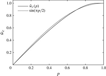
When we plot the numerical solution of (2.26) as a function of
 $p$
, we find that it is surprisingly well approximated by the simple function
 $\sin ({\rm\pi}/2p)$
(figure 5). This appears to be a coincidence, and the agreement is not perfect, but the relative difference between the approximate and exact solutions is less than 6 % for small values of
 $p$
and diminishes for larger
 $p$
. An approximation of this quality may be useful in numerical flow models as it avoids solving the nonlinear equation millions of times: for a given value of
 $p$
one may use
 $$\begin{eqnarray}\tilde{w}_{c}(p)\approx \sin ({\rm\pi}p/2).\end{eqnarray}$$
Dimensionless entrainment speed of a FC fluid in quasi-stationary flow as a function of the dimensionless parameter
 $p$
, (2.27). It is closely approximated by the function
 $\sin ({\rm\pi}p/2)$
.

The next steps are to find the shear stress and velocity profiles. The former is given by
 $$\begin{eqnarray}\displaystyle \hat{{\it\sigma}}_{xz}(h\tilde{z})\! & = & \displaystyle \!-{\it\mu}g_{z}h\,(1-\tilde{z})+K\dot{{\it\gamma}}^{2}(h\tilde{z})\nonumber\\ \displaystyle \! & = & \displaystyle \!-{\it\mu}g_{z}h\,(1-\tilde{z})+K\frac{\tilde{g}^{2}}{w_{e}^{2}}\left[1+W_{0}(-\text{exp}[-1-(1-\tilde{z})q])\right]^{2}.\end{eqnarray}$$
Recall that
 $w_{e}$
is chosen such that
 $\dot{{\it\gamma}}(0)=\dot{{\it\gamma}}_{c}$
, thus
 $\hat{{\it\sigma}}_{xz}(0)=\hat{{\it\tau}}_{c}$
. Since
 $W_{0}(-1/\text{e})=-1$
, one confirms
 $\hat{{\it\sigma}}_{xz}(h)=0$
. To find the velocity profile, we have to evaluate the integral of (2.25), with an exponential function as the argument of
 $W_{0}$
. To this end, we substitute
 $w=W_{0}(-\text{exp}(-1-q+q\tilde{z}))$
, equivalent to
 $w\text{e}^{w}=-\text{exp}(-1-q+q\tilde{z})$
with
 $w$
running from
 $w_{1}(\tilde{z}):=W_{0}(-\text{exp}(-1-q+q\tilde{z}))$
to
 $w_{2}:=W_{0}(-\text{exp}(-1-q))$
. After switching the direction of integration, the integral becomes elementary:
 $$\begin{eqnarray}u(h\tilde{z})=\frac{hg}{w_{e}}\left\{\tilde{z}-\frac{1}{2q}\left[(1+w_{2})^{2}-(1+w_{1}(\tilde{z}))^{2}\right]\right\}.\end{eqnarray}$$
One immediately confirms
 $u(0)=0$
. Ascertaining
 $u^{\prime }(h)=0$
directly from (2.30) is less straightforward, but can be accomplished by expanding the left- and right-hand sides of
 $\text{exp}(-1-q+q\tilde{z})\equiv x=w\text{e}^{w}$
around
 $\tilde{z}=1$
(or
 $x=-1/\text{e}$
) and
 $w=-1$
, respectively, and using this in the total differential of (2.30). Because of
 $w_{1}(1)=W_{0}(-1/\text{e})=-1$
and (2.24) and (2.25), one obtains the surface velocity from (2.30) as
 $$\begin{eqnarray}u(h)=\frac{hg_{x}-\hat{{\it\tau}}_{c}}{w_{e}},\end{eqnarray}$$
in agreement with what momentum conservation dictates. The same technique allows evaluation of the depth-averaged flow velocity,
 ${\bar{u}}$
, and the form factor (2.14), but the resulting expressions are lengthy and not particularly illuminating.
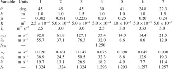
Table 3 gives examples of erosion rates and velocities as predicted by this theory. The slope angle
 ${\it\theta}$
, flow height
 $h$
, and rheological parameters
 ${\it\mu}$
and
 $K$
are typical of medium-size to large snow avalanches. Assuming an avalanche density of
 $250\ \text{kg}\ \text{m}^{-3}$
,
 ${\it\tau}_{c}$
values between 0.6 and 0.9 kPa result, which can also be considered realistic. Note that the calculated erosion speeds are the rates at which the avalanche flow depth increases (if the eroded snow is not redistributed). If the snow-cover density is
 $125\ \text{kg}\ \text{m}^{-3}$
, say, the snow cover is eroded twice as fast as indicated in the table. Cases 4, 6 and 7 are closest to the situation at the measurement location at the Vallée de la Sionne test site. With the chosen parameter values, the velocities are much lower than observed near the fluidized front, but may approximately match the velocity in the dense core of the avalanches in case 4. However, in the events we have profiling radar data of, the supply of erodible snow was already exhausted by the head of the avalanche and
 ${\it\tau}_{c}$
of the old snow was too large for erosion to occur.
Erosion speed (
 $w_{e}$
), mean and surface velocity (
 ${\bar{u}}$
,
 $u_{s}$
), and form factor (
 $f_{B}$
) for selected flow configurations of a quasi-stationary FC fluid on an inclined plane. Rows 6–8 (
 ${\bar{u}}_{0}$
,
 $u_{s,0}$
) represent non-eroding flows with the same parameters except
 $\hat{{\it\tau}}_{c}>hg_{x}$
.

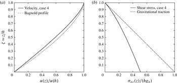
For case 4 of table 3, figure 6 compares the resulting velocity profile (normalized by its value at the flow surface) to the well-known Bagnold profile
 $1-(1-\tilde{z})^{3/2}$
that would result if there were no entrainment. The difference is qualitatively similar to the one observed for the Bingham rheology. If the gravitational traction
 $hg_{x}$
exceeds the shear strength
 $\hat{{\it\tau}}_{c}$
only slightly, the mean and surface velocity are close to the ones obtained in a non-eroding flow with the same parameters (cases 6 and 7). If the difference between
 $hg_{x}$
and
 $\hat{{\it\tau}}_{c}$
becomes substantial, the erosion speed increases and the flow velocity decreases. The velocity profiles then approach straight lines except near the surface, where they curve very sharply to satisfy the condition
 $u^{\prime }(h)=0$
. This is also reflected in the form factor, which is
 $\frac{5}{4}$
for a Bagnold profile and
 $\frac{4}{3}$
for a linear profile. Cases 1–3 and 6, 7 have
 $f_{B}$
close to
 $\frac{4}{3}$
and
 $\frac{5}{4}$
, respectively. Since
 $\dot{{\it\gamma}}(\tilde{z})\leqslant \dot{{\it\gamma}}(0)=\dot{{\it\gamma}}_{c}$
, the mean velocity is limited to
 ${\bar{u}}_{max}=h\dot{{\it\gamma}}_{c}$
. As for the Bingham fluid, the shear stress profile is curved, starting from
 $\hat{{\it\tau}}_{c}$
at
 $z=0$
– in contrast to the linear profile in a non-entraining flow.
Quasi-stationary flow of an eroding FC fluid: profiles of (a) the velocity normalized by its value at the surface and (b) the shear stress normalized by the gravitational traction
 $g_{x}h$
for parameter values of case 4 in table 3. For comparison, the Bagnold velocity profile and the shear stress in a non-entraining stationary flow (gravitational traction) are also shown. Note that the surface velocity of the entraining flow is only 60 % of the surface velocity of the non-entraining flow in this case.

3. Extension to non-stationary flows
3.1. General dynamical considerations
Gravity mass flows in nature start from rest, go through successive acceleration and deceleration phases due to the non-uniform topography, and finally come to rest again. Thus they are never in a truly (quasi-)stationary phase. Also, in reality no skimming occurs; instead, the flow depth grows, and eventually so does the velocity even on an infinitely long inclined plane. Therefore we need to address the question of how the exact solutions for quasi-stationary flows developed in § 2 can be adapted to non-stationary flow conditions. At best, one may hope to find exact solutions in very simple topographies, e.g. an infinitely long inclined plane (Eglit & Yakubenko Reference Eglit and Yakubenko2014). In cases of practical interest, i.e. with complex topography, some simplifying assumptions have to be made. However, they should be consistent with the physics and the assumptions used in deriving depth-averaged models. The uniqueness of the solutions achieved in the quasi-stationary case will be lost due to the approximations being non-unique.
In order to concentrate on the essentials, here we consider an infinitesimal column of variable mass and flow depth
 $h(t)$
moving along a path
 $Z(X)$
, parameterized by its arclength
 $s$
, at depth-averaged speed
 ${\bar{u}}(t)\equiv {\dot{s}}(t)$
. This allows us to drop terms with partial derivatives in the tangential plane, but we will account for the internal velocity profile. The flow depth may change due to erosion at the speed
 $w_{e}$
from the bed. In order to show the differences with the quasi-stationary system studied in § 2, we also allow skimming from the flow surface at the speed
 $w_{s}$
, but set
 $w_{s}=0$
afterwards. The equation of motion involves gravitational driving, the specific bed shear stress
 $\hat{{\it\sigma}}_{xz}\leqslant \hat{{\it\tau}}_{c}$
, and the decelerating effect of entraining mass from rest and losing mass moving at the speed
 $u(h)>{\bar{u}}$
:
 $$\begin{eqnarray}\displaystyle & \displaystyle {\dot{h}}=w_{e}-w_{s}, & \displaystyle\end{eqnarray}$$
 $$\begin{eqnarray}\displaystyle & \displaystyle \dot{{\bar{u}}}=g_{x}-\text{sgn}({\bar{u}})\frac{\left|\hat{{\it\sigma}}_{xz}^{(b)}\right|}{h}-(w_{e}-w_{s})\frac{{\bar{u}}}{h}-w_{s}\frac{u(h)}{h}, & \displaystyle\end{eqnarray}$$
 $$\begin{eqnarray}\displaystyle & \displaystyle \left|\hat{{\it\sigma}}_{xz}^{(b)}\right|=\left\{\begin{array}{@{}ll@{}}\displaystyle \hat{{\it\tau}}_{y}+\frac{6}{(3-r)r}{\it\nu}_{B}\frac{|{\bar{u}}|}{h},\quad & {\bar{u}}<{\bar{u}}_{thr}\ \text{(Bingham fluid),}\\ \displaystyle {\it\mu}g\cos {\it\theta}+K\left(\frac{5{\bar{u}}}{2h}\right)^{2},\quad & {\bar{u}}<{\bar{u}}_{thr}\ \text{(FC fluid),}\\ \hat{{\it\tau}}_{c},\quad & {\bar{u}}\geqslant {\bar{u}}_{thr}.\end{array}\right. & \displaystyle\end{eqnarray}$$
 $\tilde{r}$
is the sheared fraction of the flow depth, see § 2.1. In the quasi-stationary case (
 $qs$
) treated previously, erosion at the bed was balanced by skimming at the surface,
 $w_{e}^{qs}=w_{s}^{qs}$
, thus
 $h=\text{const.}$
from (3.1). In contrast, the non-stationary case (
 $ns$
) is characterized by
 $w_{s}^{ns}=0$
. If entrainment occurs, the equation of motion becomes
 $$\begin{eqnarray}g_{x}-\text{sgn}({\bar{u}})\frac{\hat{{\it\tau}}_{c}}{h}=\left\{\begin{array}{@{}ll@{}}\displaystyle \frac{w_{e}^{qs}\,u(h)}{h}\quad & \text{(quasi-stationary)},\\ \displaystyle \frac{w_{e}^{ns}\,{\bar{u}}}{h}+\dot{{\bar{u}}}\quad & \text{(non-stationary)}.\end{array}\right.\end{eqnarray}$$
In the stationary case, the problem consisted of finding
 $w_{e}^{qs}$
and
 $u(h)$
for a given value of their product. The non-stationary case raises the additional problem of apportioning the excess specific shear stress
 $hg_{x}-\hat{{\it\tau}}_{c}$
between entrainment (
 $w_{e}^{ns}{\bar{u}}$
) and acceleration (
 $h\dot{{\bar{u}}}$
).
Simply setting
 $w_{e}^{ns}({\bar{u}},{\it\theta},h,\hat{{\it\tau}}_{c})\approx w_{e}^{qs}({\it\theta},h,\hat{{\it\tau}}_{c})$
in (3.4) is a poor choice because the entrainment rate is determined by the stress gradient at the interface between bed and flow, which depends strongly on the flow velocity. In the following, we will discuss two possible extensions based on different approximations, one for the Bingham fluid and another for the FC fluid. While they cannot claim the same degree of rigour as the results obtained so far, they can be applied to real-world problems and eventually compared to numerical approaches that resolve the bed-normal dimension (Crosta et al.
Reference Crosta, Imposimato and Roddeman2009b
; Issler & Pastor Pérez Reference Issler and Pastor Pérez2011; Eglit & Yakubenko Reference Eglit and Yakubenko2014).
For completeness, we state the full set of equations for a quasi-three-dimensional depth-averaged flow model (with
 $w_{s}=0$
). The fields
 $h(\boldsymbol{x},t)$
and
 $\boldsymbol{u}(\boldsymbol{x},t)\equiv (u_{x}(x,y,t))$
,
 $u_{y}((x,y,t))$
replace
 $h(t)$
and
 ${\dot{s}}(t)$
. Neglecting curvature-dependent terms for simplicity, we obtain the mass balance and the momentum balance in conservative form,
 $$\begin{eqnarray}\displaystyle & \partial _{t}h+\partial _{j}(h{\bar{u}}_{j})=w_{e}(h,{\bar{u}}_{k},x_{l}), & \displaystyle\end{eqnarray}$$
 $$\begin{eqnarray}\displaystyle & \partial _{t}(h{\bar{u}}_{i})+\partial _{j}(h\overline{u_{i}u_{j}})=hg_{i}+\partial _{j}(h\hat{\bar{{\it\sigma}}}_{ij})-\hat{{\it\sigma}}_{iz}^{(b)}. & \displaystyle\end{eqnarray}$$
 $i$
,
 $j$
,
 $k$
,
 $l$
take the values
 $x$
,
 $y$
, and summation over repeated indices is understood. In (3.6), the stresses are averaged over the flow depth except for the bed shear stress
 $\hat{{\it\sigma}}_{iz}^{(b)}$
, and the momentum flux term can be expressed in terms of
 ${\bar{u}}_{i}$
and the (unknown) form factor
 $f_{B}$
as
 $h\overline{u_{i}u_{j}}=f_{B}h{\bar{u}}^{2}$
. The term proportional to
 $w_{e,s}$
in (3.2), quantifying the deceleration of the flow due to the acceleration of the entrained mass from rest to the flow velocity, does not appear explicitly in (3.6); it is recovered, however, if one transforms the momentum balance equation into the equation of motion by substituting the mass balance equation into it. Also note that (2.2) should be extended to
 $$\begin{eqnarray}w_{e}(x,y,t)\dot{{\it\gamma}}(x,y,z,t)=\frac{u_{i}}{|\boldsymbol{u}|}\left[g_{i}(x,y)+\partial _{j}\hat{{\it\sigma}}_{ij}(x,y,z,t)+\partial _{z}\hat{{\it\sigma}}_{iz}(x,y,z,t)\right]\end{eqnarray}$$
(with summation over the indices
 $i,j\in \{1,2\}$
) when normal-stress gradients occur.
3.2. Approximate solution for the Bingham fluid
A central ingredient in the present theory of erosion and entrainment is the assumed brittle behaviour of the bed material, which locks the bed shear stress at the value of the bed shear strength,
 ${\it\tau}_{c}$
. For a given rate-dependent rheology, this determines the shear rate at the bed–flow interface,
 $\dot{{\it\gamma}}_{c}$
, independent of the depth-averaged flow velocity,
 ${\bar{u}}$
. The derivative of the shear rate, however, is linked to the flow velocity, and at the same time it is a determining factor in the equation for the erosion rate, see (2.2). (Note that Issler & Pastor Pérez Reference Issler and Pastor Pérez2011 derived this equation for a non-stationary flow.) There is a one-to-one relation between
 $\dot{{\it\gamma}}^{\prime }(0)$
and
 ${\bar{u}}$
in the quasi-stationary case, but not in the non-stationary case.
In order to obtain an approximate erosion rate for non-stationary flows, we therefore need to make a reasonable assumption concerning the derivative of the shear rate at the bed–flow interface. To this end, at any given time we adopt the velocity profile of a quasi-stationary eroding ‘proxy’ flow with the same flow depth, shear-layer depth and critical shear rate. However, we use a different viscosity
 ${\it\nu}^{\prime }$
for the depth-averaged velocities to match between the original non-stationary flow and the proxy flow. In calculating the erosion speed, we use the original value of
 ${\it\nu}$
. Conceptually, this is analogous to the assumption, routinely made in depth-averaged flow models without entrainment, that the velocity profile is identical to that of an equilibrium flow with the same velocity.
The approximating profile function
 $v(z,t)$
has to satisfy four conditions: (i) no slip at the interface,
 $v(0,t)=0$
, (ii) vanishing shear in the plug layer,
 $\partial _{z}v(z,t)=0$
for
 $z\geqslant r$
, (iii) critical shear stress for erosion at the interface,
 $\partial _{z}v(0,t)=\dot{{\it\gamma}}_{c}$
, and (iv) matching depth-averaged velocities between the non-stationary flow and quasi-stationary proxy flow,
 $\bar{v}(t)={\bar{u}}(t)$
. The first and second conditions are automatically fulfilled by the solution (2.11) if
 $r$
or, equivalently,
 $\tilde{r}\equiv r/h$
match between the two flows. Applying the scaling of (2.13) with the viscosity
 ${\it\nu}^{\prime }$
, we obtain the depth-averaged velocity as
 $$\begin{eqnarray}\frac{{\it\nu}^{\prime }{\bar{u}}}{h^{2}g_{x}}=\frac{\tilde{r}}{{\it\chi}}\left(1-\frac{\tilde{r}}{2}\right)+\frac{\tilde{r}}{{\it\chi}^{2}}-\frac{1+{\it\chi}}{{\it\chi}^{3}}(1-\text{e}^{-\tilde{r}{\it\chi}}).\end{eqnarray}$$
(We write
 ${\it\chi}$
instead of
 $\tilde{w}_{e}$
to emphasize that this equation does not give us the entrainment rate of the non-stationary flow.) Now we implement the condition (iii) stated above and find
 $1-\text{e}^{-\tilde{r}{\it\chi}}={\it\chi}{\it\nu}^{\prime }\dot{{\it\gamma}}_{c}/(hg_{x})$
, giving us
 ${\it\nu}^{\prime }$
in terms of
 ${\it\chi}$
. By substituting this in (3.8) and rearranging terms, we obtain the following equation for
 ${\it\chi}$
:
 $$\begin{eqnarray}0=F({\it\chi})\equiv \left\{\begin{array}{@{}ll@{}}\displaystyle \left(\frac{1+{\it\chi}}{{\it\chi}^{2}}+{\it\alpha}\right)(1-\text{e}^{-\tilde{r}{\it\chi}})-\frac{\tilde{r}}{{\it\chi}}-\left(1-\frac{\tilde{r}}{2}\right)\tilde{r},\quad & {\it\chi}\neq 0,\\ 0,\quad & {\it\chi}=0.\end{array}\right.\end{eqnarray}$$
Again, this is a transcendental equation – this time depending on the dimensionless parameter
 ${\it\alpha}\equiv {\bar{u}}/(h\dot{{\it\gamma}}_{c})$
– and needs to be solved numerically. We can substitute
 ${\it\chi}({\it\alpha})$
into the expression for
 $\dot{{\it\gamma}}^{\prime }(0)$
,
 $$\begin{eqnarray}\dot{{\it\gamma}}^{\prime }(0)=-\frac{\dot{{\it\gamma}}_{c}}{h}\,\frac{{\it\chi}}{\text{e}^{\tilde{r}{\it\chi}}-1},\end{eqnarray}$$
and obtain the erosion rate by evaluating (2.2) at
 $z=0$
:
 $$\begin{eqnarray}w_{e}=\max \left(0,\frac{g_{x}}{\dot{{\it\gamma}}_{c}}-\frac{{\it\nu}}{h}\,\frac{{\it\chi}({\it\alpha})}{\text{e}^{\tilde{r}{\it\chi}({\it\alpha})}-1}\right).\end{eqnarray}$$
If the depth-averaged velocity is equal to that of the quasi-stationary flow,
 ${\bar{u}}={\bar{u}}_{qs}$
and
 ${\it\alpha}={\it\alpha}_{qs}$
, then
 ${\it\nu}^{\prime }={\it\nu}$
in (3.8) and
 ${\it\chi}({\it\alpha}_{qs})=\tilde{w}_{e}^{qs}$
. Recalling the scaling of
 $w_{e}$
and that
 ${\it\nu}\dot{{\it\gamma}}_{c}/(hg_{x})=\tilde{{\it\tau}}_{c}-\tilde{{\it\tau}}_{y}$
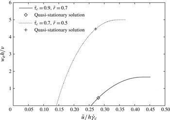
, one verifies that (3.11) recovers the erosion speed of the quasi-stationary flow, given by (2.15). This is exemplified in figure 7, where the corresponding solutions of the quasi-stationary equations are marked by symbols.
The dimensionless erosion speed
 $w_{e}h/{\it\nu}$
of a Bingham fluid as a function of the dimensionless depth-averaged velocity
 ${\it\alpha}={\bar{u}}/(h\dot{{\it\gamma}}_{c})$
for two combinations of the dimensionless bed shear strength,
 $\tilde{{\it\tau}}_{c}=\hat{{\it\tau}}_{c}/(hg_{x})$
, and the relative shear-layer depth,
 $\tilde{r}=r/h$
. The points corresponding to the solutions of the corresponding quasi-stationary systems are marked with symbols. The curves end at the maximum value of
 ${\it\alpha}$
that is compatible with the chosen value of
 $\tilde{r}$
.

The maximum function appears in (3.11) because we demand the erosion rate to be positive for the reasons discussed in § 1.3. However, this condition is not equivalent to the condition
 ${\it\chi}>0$
, which separates velocity profiles that are straighter (
 ${\it\chi}>0$
) or more rounded (
 ${\it\chi}<0$
) than a parabolic profile, respectively. The threshold velocity can be determined from (3.11) and (3.8): some algebra on (3.11) shows the threshold value of
 $\tilde{w}_{e}$
to be
 $\tilde{w}_{e}^{thr}=-(\tilde{{\it\tau}}_{c}+\tilde{r}-1)^{-1}$
, which can be substituted into (3.9) to obtain
 ${\bar{u}}_{thr}$
.
Figure 7 shows plots of the erosion speed (3.11), scaled with
 ${\it\nu}/h$
, versus the depth-averaged velocity (3.8), scaled with
 $h\dot{{\it\gamma}}_{c}$
, for two combinations of the shear-layer depth
 $r$
divided by
 $h$
and the bed shear strength divided by
 $hg_{x}$
. The graphs end at
 ${\bar{u}}/(h\dot{{\it\gamma}}_{c})=\tilde{r}(1-\tilde{r}/2)$
, which is the limit velocity for flows with convex velocity profiles, as we have assumed here. The corresponding limit value of the erosion speed is
 $w_{e}h/{\it\nu}=(\tilde{{\it\tau}}_{c}+\tilde{r}-1)^{-1}$
.
3.3. Approximate solution for the frictional–collisional fluid
For the FC rheology, we explore a different approach. Rather than matching profile functions of a quasi-stationary eroding flow to the depth-averaged velocity and critical shear rate of the actual non-stationary flow, we approximate the profile function directly. The numerical simulations of accelerating flows by Issler & Pastor Pérez (Reference Issler and Pastor Pérez2011) as well as the results of § 2.2 show that the profiles approach the straight line
 $u_{\infty }(z)=\dot{{\it\gamma}}_{c}z$
as the erosive power (and the velocity in the case of non-stationary flows) increases. The profiles become increasingly curved near
 $\tilde{z}=1$
. The two-parameter family of functions
 $$\begin{eqnarray}v(h\tilde{z})=U({\bar{u}},\dot{{\it\gamma}}_{c})[1-(1-\tilde{z})^{{\it\beta}({\bar{u}},\dot{{\it\gamma}}_{c})}],\quad {\it\beta}>1,\end{eqnarray}$$
captures this behaviour.
 $U$
, the surface velocity of the flow, and the exponent
 ${\it\beta}$
depend on variables of the actual non-stationary flow.
As in the case of the Bingham fluid, the first and second of the four conditions (i)
 $v(0,t)=0$
, (ii)
 $\partial _{z}v(h,t)=0$
, (iii)
 $\partial _{z}v(0,t)=\dot{{\it\gamma}}_{c}$
, and (iv)
 $\bar{v}(t)={\bar{u}}(t)$
are automatically fulfilled by the functional form (3.12) if
 ${\it\beta}>1$
. One easily calculates
 $\partial _{z}v|_{z=0}={\it\beta}U/h$
and
 ${\bar{u}}={\it\beta}/({\it\beta}+1)\,U$
. Substituting the latter relation into the former and equating
 $\partial _{z}v$
to
 $\dot{{\it\gamma}}_{c}$
, we obtain
 $$\begin{eqnarray}{\it\beta}=\frac{h\dot{{\it\gamma}}_{c}}{{\bar{u}}}-1.\end{eqnarray}$$
The admissible range of
 ${\it\beta}$
leads to a restriction for the depth-averaged velocity,
 $$\begin{eqnarray}\frac{{\bar{u}}}{h\dot{{\it\gamma}}_{c}}<\frac{1}{2},\end{eqnarray}$$
the limit corresponding to a straight-line velocity profile. Values of
 ${\it\beta}$
larger than the Bagnoldian value of
 $\frac{3}{2}$
may arise, e.g. during start-up of the flow: the velocity profile evolves progressively from a plug-like shape with very high values of curvature near the bottom towards nearly linear profiles with the curvature concentrated at the top. Similarly, when a flow enters a steeper segment of the path,
 ${\it\beta}$
will initially increase rapidly, possibly beyond
 $\frac{3}{2}$
, and then diminish again as the flow adjusts to the new conditions.
The approximate erosion rate of the non-stationary flow follows from (2.2):
 $$\begin{eqnarray}w_{e}({\bar{u}})\approx {\it\Theta}({\bar{u}}-{\bar{u}}_{thr})\,w_{e,\infty }\left(1-\frac{{\bar{u}}_{thr}}{{\bar{u}}}\right),\quad {\bar{u}}<\frac{1}{2}h\dot{{\it\gamma}}_{c}.\end{eqnarray}$$
The scale for the entrainment speed is set by
 $$\begin{eqnarray}w_{e,\infty }=\frac{h(g_{x}+{\it\mu}g_{z})+4K\dot{{\it\gamma}}_{c}^{2}}{h\dot{{\it\gamma}}_{c}},\end{eqnarray}$$
but the actual entrainment speed is always smaller by a finite amount because
 ${\bar{u}}$
is limited. It grows as a nonlinear function of
 ${\bar{u}}$
from zero at the threshold velocity
 $$\begin{eqnarray}{\bar{u}}_{thr}=\frac{h\dot{{\it\gamma}}_{c}}{2}\,\frac{K\dot{{\it\gamma}}_{c}^{2}}{h(g_{x}+{\it\mu}g_{z})+4K\dot{{\it\gamma}}_{c}^{2}}\end{eqnarray}$$
to its maximum value
 $(g_{x}+{\it\mu}g_{z})/\dot{{\it\gamma}}_{c}$
at
 ${\bar{u}}=h\dot{{\it\gamma}}_{c}/2$
. Here
 ${\bar{u}}_{thr}$
may differ significantly from the value
 $\frac{2}{5}h\dot{{\it\gamma}}_{c}$
obtained by using the non-eroding equilibrium velocity profile. The exponent
 ${\it\beta}$
has been eliminated from (3.15), but can be recovered from (3.13) for calculating the form factor
 $f_{B}=({\it\beta}+1)/({\it\beta}+1/2)$
. Erosion is possible for
 $hg_{x}>\hat{{\it\tau}}_{c}-5K\dot{{\it\gamma}}_{c}^{2}$
if the velocity is high enough, but if the slope is too gentle, the flow is decelerated and erosion will stop eventually.
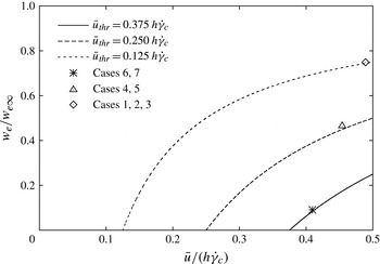
Figure 8 shows the non-dimensional approximate erosion speed
 $w_{e}/w_{e\infty }$
as a function of the non-dimensional depth-averaged velocity
 ${\bar{u}}/(h\dot{{\it\gamma}}_{c})$
for three different values of the non-dimensionalized threshold velocity
 $2{\bar{u}}_{thr}/(h\dot{{\it\gamma}}_{c})$
. Note that the curves do not pass precisely through the points corresponding to solutions of the quasi-stationary problem because the ansatz functions (3.12) do not capture the quasi-stationary profile exactly, but the agreement is satisfactory.
Approximate velocity dependence of the erosion speed in the case of the FC rheology, for three different values of the threshold velocity. All quantities are scaled by
 $w_{e,\infty }$
and
 $h\dot{{\it\gamma}}_{c}$
, respectively. The symbols mark the quasi-stationary erosion rates of the corresponding example cases listed in table 3.

We may gain some insight into the properties of this formula by considering the asymptotic behaviour of the model consisting of (3.1), (3.2) and (3.15) in the case
 ${\it\mu}=0$
. (With
 ${\it\mu}>0$
, the model eventually breaks down as the flow depth increases, see § 4.2.) If there is a solution for which the erosion rate tends to a constant value, the flow depth tends to linear growth in time,
 $h\sim w_{e}t$
, and becomes very large. As a consequence, the bed resistance term in (3.2) becomes negligible and the equation of motion simplifies to
 $$\begin{eqnarray}\dot{{\bar{u}}}\simeq g_{x}-\frac{{\bar{u}}}{t},\end{eqnarray}$$
solved by
 ${\bar{u}}(t)\simeq g_{x}t/2$
, i.e. constant acceleration at half the value of the component of the gravitational acceleration along the slope (Issler & Pastor Pérez Reference Issler and Pastor Pérez2011). Eglit & Yakubenko (Reference Eglit and Yakubenko2014) showed that this asymptotic solution has a linear velocity profile and that the flow particles accelerate at the rate
 $g_{x}$
, i.e. at twice the rate of the centre of mass. The asymptotic velocity corresponds to the limit velocity for which the model ceases to be applicable (the limit itself growing linearly with the flow depth). Inserting the limits of (3.16) and (3.17), one sees that
 $w_{e}\rightarrow w_{e,\infty }$
as
 $h\rightarrow \infty$
and
 $$\begin{eqnarray}w_{e,\infty }\mathop{\longrightarrow }\limits_{h\rightarrow \infty }\frac{g_{x}}{\dot{{\it\gamma}}_{c}}=g_{x}\sqrt{\frac{K}{\hat{{\it\tau}}_{c}}}.\end{eqnarray}$$
With the values from table 1 in Issler & Pastor Pérez (Reference Issler and Pastor Pérez2011) and
 $g=10.0\ \text{m}\ \text{s}^{-2}$
, one finds
 $w_{e,\infty }=0.161\ \text{m}\ \text{s}^{-1}$
, which agrees with the result from the numerical simulation (figure 3e in Issler & Pastor Pérez Reference Issler and Pastor Pérez2011). Furthermore, the fact that the erosion speed tends to
 $w_{e,\infty }$
implies that the velocity profile becomes linear asymptotically.
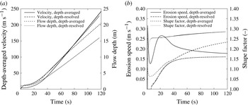
We can compare the present model in detail with the published depth-resolved simulation by solving the mass-point equations (3.1) and (3.2) for the same parameter values, i.e.
 ${\it\mu}=0$
,
 $K=0.005\ \text{m}^{2}$
, initial depth (normal to the slope)
 $h_{0}=1.05\ \text{m}$
,
 ${\it\rho}_{f}=300\ \text{kg}\ \text{m}^{-3}$
,
 ${\it\tau}_{c}=1450\ \text{kPa}$
, and constant inclination angle
 ${\it\theta}=30^{\circ }$
. The actual model implementation differs somewhat from those equations (see appendix B for details), but this is of no consequence in the present context.
Figure 9(a) shows erosion to start at a lower velocity in the depth-averaged model than in the depth-resolved one. For this reason, the velocity grows more slowly in the initial phase than in the depth-resolved simulation. Asymptotically, however, the acceleration of the centre of mass tends to
 $(g\sin {\it\theta})/2$
in both models. The erosion speeds also tend to the same value, but the approach to the asymptotic value differs strongly between the models (figure 9
b):
 $w_{e}$
is a monotonically increasing function of time in the depth-resolved model. In the approximate analytic erosion model, it rapidly jumps to a value about twice as large as
 $w_{e,\infty }$
after the threshold speed is crossed, then drops approximately 20 % below
 $w_{e,\infty }$
, reaches another local maximum and finally approaches
 $w_{e,\infty }$
from above. Accordingly, the flow depth is approximately 25 % larger after a drop of 10 km (figure 9
a). This discrepancy between the models is closely related to the shape of the velocity profile, as figure 9(b) reveals: the depth-resolved model computes a profile close to the equilibrium Bagnold shape with
 $f_{B}$
slowly growing from
 $\frac{5}{4}$
to
 $\frac{4}{3}$
. In contrast, the depth-averaged flow has a blunter shape than the Bagnold profile
 $(\,f_{B}=\frac{5}{4})$
during the entire simulation, but will cross-over to an increasingly linear profile if given enough time. Why the approximate model chooses blunt profiles and how it can be modified to agree more closely with the depth-resolved model remains to be investigated.
Avalanche flow on a 30° slope as simulated with a slab model for the FC rheology and the erosion formula (3.15), compared to a depth-resolved simulation presented by Issler & Pastor Pérez (Reference Issler and Pastor Pérez2011). See the text for the parameter values. (a) Velocity (left scale) and flow depth (right scale). (b) Erosion speed (relative to flow density, left scale) and shape factor
 $f_{B}$
(right scale) from the depth-averaged and depth-resolved models. Low values of
 $f_{B}$
correspond to blunt, plug-like velocity profiles.

4. Discussion and outlook
4.1. Implications of the proposed erosion and entrainment theory
Perhaps the most fundamental result of the present work is the proof of concept that erosion and entrainment in depth-averaged models of GMFs can be formulated in a mathematically self-consistent and physically meaningful way. This is not a priori obvious because depth-averaging discards information about the state of the system at and near the bed–flow interface, and it is precisely there that the erosion rate is determined.
Two additional hypotheses helped to make the problem tractable: first, the mechanical problem becomes much simpler if we assume the bed to be perfectly brittle, with a characteristic shear strength
 ${\it\tau}_{c}$
. We argued that this is a reasonable approximation for snow. The central role of this hypothesis in the present approach suggests testing its applicability in other types of cohesive substrates overflowed by GMFs, like soil with a substantial content of silt and clay. In this context, excess pore pressure generated by the flow-induced shearing of the soil may be an important factor (Iverson Reference Iverson2012) that necessitates a different approach.
Secondly, the brittleness assumption suggests adopting an analogue of Owen’s (Reference Owen1964) hypothesis, stipulating that the interfacial shear stress is locked at the critical value
 ${\it\tau}_{c}$
whenever there is erosion. The validity of this hypothesis cannot be proved or refuted in the framework of depth-averaged models, but it might be possible to study this question through discrete-element simulations if the frictional granular bed can be modified so as to exhibit a finite yield strength at vanishing normal load (Rognon et al.
Reference Rognon, Roux, Naaim and Chevoir2008).
Despite its unrealistic features, the toy model introduced in Issler & Jóhannesson (Reference Issler and Jóhannesson2006) and developed further in § 2 proved to be invaluable because it constrains the system to the point where it becomes rigorously solvable. It is an open question at present what other rheological models can be solved in this way, and it should be worthwhile to explore this direction further. A particularly interesting candidate rheology is the Jop–Forterre–Pouliquen model for granular materials (Jop, Forterre & Pouliquen Reference Jop, Forterre and Pouliquen2006).
The explicit analytic solutions (even though in terms of non-elementary functions) of the quasi-stationary problem were very helpful both in developing a numerical approach (Issler & Pastor Pérez Reference Issler and Pastor Pérez2011) and to find analytical extensions to non-stationary flows. Sections 3.2 and 3.3 illustrate that this process is not uniquely determined. It should be illuminating to approximately parameterize the numerical solutions for non-stationary flow of a Bingham fluid presented by Eglit & Yakubenko (Reference Eglit and Yakubenko2014) in a similar way as was done in § 3.3, or to adapt quasi-stationary eroding solutions of the FC model to the non-stationary case, as we did for the Bingham fluid in § 3.2.
Extensive comparison of the predictions of this theory to measurements is not at present possible. On the one hand, there do not seem to be any laboratory experiments studying entrainment from a brittle cohesive bed into a flow describable by the rheologies studied in this paper. On the other hand, full-scale measurements to date (mainly on snow avalanches) have not measured all the parameters that are needed to determine the flow rheology and the bed properties. The preliminary back-calculation (appendix B) of a small avalanche whose deposits were studied in great detail exemplifies this: at first sight, the model underestimates the erosion rate greatly. However, if our interpretation of the event (appendix A) is correct, most of the eroded mass was not really entrained into the flow and the simplistic slab model may in fact estimate the entrainment rate fairly well. However, this cannot be ascertained because the bed shear strength, which plays a central role in our model, was not measured and we had to guess it.
4.2. Validity limits of the theory
At several points in this paper, limitations of the applicability of the presented approach became apparent from physical considerations or mathematical analysis. These limitations can be traced back to the assumptions that erosion is gradual and that there is a critical shear strength of the snow pack. Together, they limit the shear rate to values below the critical value at the interface,
 $\dot{{\it\gamma}}_{c}$
. Since the shear rate decreases with increasing distance from the bed, the depth-averaged flow velocity is strictly limited.
Further restrictions arise because the shear stress exerted by an avalanche at rest must be less than
 ${\it\tau}_{c}$
in the model. For the Bingham fluid, this implies
 ${\it\tau}_{y}<{\it\tau}_{c}$
, but does not restrict the flow depth. The FC rheology contains a Coulomb friction term, which limits the flow depth to
 $h<{\it\tau}_{c}/({\it\mu}g\cos {\it\theta})$
. An eroding avalanche on an inclined plane will eventually exceed this limit, but the theory ceases to apply even before this point is reached: as
 $h$
grows,
 $\dot{{\it\gamma}}_{c}$
decreases towards 0, and so
 ${\bar{u}}_{max}=h\dot{{\it\gamma}}_{c}/2$
will at some point fall below
 ${\bar{u}}$
, which is increasing.
We qualitatively discuss what probably happens in an FC avalanche beyond this point; detailed study and mathematical modelling must be deferred to future work, however. Due to the growth of
 $h$
,
 $\dot{{\it\gamma}}_{c}$
decreases, but this is felt only near the bottom of the flow while the upper layers continue to accelerate. The decrease of
 $\dot{{\it\gamma}}_{c}$
directly leads to a pronounced increase of
 $w_{e}$
. The velocity profile is originally convex throughout the entire flow depth, but this cannot be maintained: it remains convex near the top, but becomes concave near the bottom. The family of profile functions (3.12) cannot accommodate this shape, hence the breakdown of the approximate model. It remains to be seen whether approximate profile functions can be constructed that capture this transition while still leading to tractable equations.
However, even if one succeeds in this regard, the system will reach the point where the Coulomb friction alone overwhelms the shear strength of the bed. The condition
 $\dot{{\it\gamma}}|_{z=0}=\dot{{\it\gamma}}_{c}$
cannot be maintained as
 $\dot{{\it\gamma}}|_{z=0}$
would become imaginary. The only possible reaction of the system seems to be catastrophic failure of the bed over a finite depth
 ${\rm\Delta}b$
down to a layer where the strength matches the load; this is the erosion mechanism termed ripping in § 1.1. One can probably consider this slab fully disintegrated if it is perfectly brittle as assumed hitherto, and treat it as an FC fluid. The shear stress at
 $z=0$
, which no longer is constrained at the value
 ${\it\tau}_{c}(0)$
, will progressively accelerate the eroded mass, the velocity profile being concave near
 $z=0$
initially. Over time, the shear stress at the new interface
 $z=-{\rm\Delta}b$
may grow to the value
 ${\it\tau}_{c}(-{\rm\Delta}b)$
as the velocity of the eroded slab and the shear rate increase, and then erosion by scour or by ripping resumes.
If future work confirms these conjectures, the failure of the model at
 ${\bar{u}}=h\dot{{\it\gamma}}_{c}/2$
is reminiscent of a second-order phase transition that is not captured by the model: all physical quantities like the velocity or the erosion rate evolve continuously, but the character of the profile of the shear rate changes discontinuously from monotonic to non-monotonic. In contrast, the breakdown at
 $\dot{{\it\gamma}}_{c}\rightarrow 0$
has the characteristics of a first-order phase transition where the erosion rate diverges and then drops to zero while the flow depth increases by a step. Thus the approximate non-stationary FC erosion model needs to be amended to (i) incorporate profiles with an inflection point and (ii) accommodate discontinuous changes in the flow depth.
4.3. Steps towards practical applications
In hazard mapping, the central task is to predict the run-out distance and other properties of (future) mass-flow events with long return periods. Practical application of the presented erosion models in such a context will therefore, among other parameters, require knowledge of the likely spatial distribution of brittle shear strength during the first few days after snow storms, when most avalanches are released. One has to expect that these values depend significantly on the snow climate, the altitude, the exposure to radiation and wind, and the return period. These dependences need to be investigated through extensive field measurements. For example, snow around the fjords in western Norway typically is warm and humid near sea level, but under exceptional conditions it may be cold and have low cohesion along the entire avalanche path. Under such conditions, avalanches have run more than a kilometre further than usual (Lied et al.
Reference Lied, Instanes, Domaas, Harbitz and Hestnes1998). Also, the shear strength of snow increases significantly with depth in the snow pack. The complex relationships governing this effect need to be distilled into simple formulae so that the numerical model can compute the instantaneous shear strength
 ${\it\tau}_{c}(x,y,b(t))$
as erosion progresses.
Our preliminary attempt at back-calculating a real avalanche event with the proposed erosion formula for FC flows (appendix B) exemplifies that the inclusion of entrainment renders the system highly nonlinear and sensitive to the initial and boundary conditions. We therefore anticipate that – even if we had the perfect model available – it will take a substantial effort to establish practical procedures that allow predictive and reliable simulations to be carried out.
As mentioned in § 1.1, there are other important erosion mechanisms besides scour. The back-calculation of the small avalanche event in appendix B indicates that ripping may affect much larger masses than scour even though it had little influence on the flow dynamics in that case. Meaningful validation and application of the model will probably only be possible when all erosion modes are included in a more comprehensive model. That entrainment model should then be implemented, not in a slab model, but in a fully fledged quasi-three-dimensional code.
Finally, the present study shows how erosion and entrainment are inextricably linked to the flow rheology. This conclusion has immediate consequences for experimental studies of entrainment: experiments have to be devised such that the rheology of the flow can be determined simultaneously with the erosion rate and information on the erosion mechanism gained. This is a great challenge, but if progress can be made, it will give answers simultaneously to the two main problems in GMF dynamics.
Acknowledgements
In the long course of research leading to this paper, I have enjoyed stimulating discussions with M. Barbolini, J. Eggenhuisen, M. E. Eglit, J.-T. Fischer, P. Gauer, K. Hutter, C. G. Johnson, K. Lied, M. Y. Louge, D. M. McClung, M. Naaim, H. Norem, G. Parker, M. Pastor, F. Sandersen and B. Sovilla. In particular, T. Jóhannesson collaborated in the early stages and untiringly scrutinized a large number of drafts. J. N. McElwaine pointed out the connection to Lambert’s
 $W$
function, which streamlined the mathematics considerably. He and two anonymous referees provided much appreciated reviews that improved the paper significantly. I am indebted to J. T. Jenkins, E. Meiburg and A. Valance for the stimulating atmosphere during the GeoFlows13 workshop at the Kavli Institute for Theoretical Physics at the University of California at Santa Barbara and to S. Sassa and the Soil Dynamics Group of the Port and Airport Research Institute in Yokosuka, Japan for their kind hospitality during the final research and write-up stage. Financing for this work came from the European Commission through the FP5 project Avalanche Studies and Model Validation in Europe (SATSIE, contract no. EVG1-CT2002-00059), the Swiss National Science Foundation (project Avalanche Dynamics: on-site studies, modeling and practical applications, grant no. 101911), the Norwegian government through the Snow Research grant to NGI, and an NGI research fellowship.
Appendix A. Brief overview of experimental knowledge and constraints on erosion and entrainment
In debris flows (mixtures of water, fine sediment and possibly clasts up to boulder size), the occurrence of bed erosion and deposition and the significance of these processes for the flow dynamics is immediately obvious to an observer, see e.g. Breien et al. (Reference Breien, De Blasio, Elverhøi and Høeg2008) and Mangeney et al. (Reference Mangeney, Roche, Hungr, Mangold, Faccanoni and Lucas2010). Also in all other types of rapid or extremely rapid GMFs, the flowing mass can change greatly. Already by the end of the 1960s, researchers at Moscow State University had recognized the importance of entrainment in snow avalanches and developed models to describe this process in the framework of depth-averaged continuum models (Briukhanov et al. Reference Briukhanov, Grigorian, Miagkov, Plam, Shurova, Eglit, Yakimov and Ôura1967; Eglit Reference Eglit1968; Grigorian & Ostroumov Reference Grigorian and Ostroumov1977). These early dynamical models were tested with considerable success against measurements from instrumented test sites in the Caucasus and the Khibiniy mountains, although detailed testing of the proposed entrainment mechanisms was not possible with the experimental techniques available at the time.
Surprisingly, the work of the Moscow group – and the problem of entrainment and deposition in general – were largely ignored in other countries for decades. On the modelling side, notable exceptions were Brugnot & Pochat (Reference Brugnot and Pochat1981), Gubler (Reference Gubler, Salm and Gubler1987), Maeno & Nishimura (Reference Maeno and Nishimura1987) and Norem & Schieldrop (Reference Norem and Schieldrop1991). Cannon & Savage (Reference Cannon and Savage1988) may have been the first to include an (a priori defined) erosion rate in a run-out model for debris flows. The theory of self-igniting turbidity currents by Parker, Fukushima & Pantin (Reference Parker, Fukushima and Pantin1986), as well as some models of powder-snow avalanche motion inspired by that work, included empirical expressions for the erosion rate (e.g. Fukushima & Parker Reference Fukushima and Parker1990; Hermann et al. Reference Hermann, Issler, Keller, Wagner, Hirschel, Périaux and Piva1994).
Field observations of erosion in GMFs or dedicated experiments continued to be lacking, however. Issler et al. (Reference Issler, Gauer, Schaer and Keller1996) highlighted the importance of entrainment and deposition in the non-dense part of snow avalanches on the basis of field investigations. The detailed measurements of local mass balance along the Monte Pizzac avalanche path (Italian Dolomites) by Sovilla et al. (Reference Sovilla, Sommavilla and Tomaselli2001) finally rekindled widespread interest in the issue by showing that the flowing mass increased by up to an order of magnitude over the release mass in some cases. The important achievement of that work was that both the eroded and deposited mass were determined at approximately 15 cross-sections of the path, taking into account the densities of the original snow cover, the dense deposits and the somewhat compacted substrate. Erosion and deposition rates were found to vary substantially between events due to different snow conditions and avalanche sizes. These small avalanches of less than 500 t maximum mass eroded
 $50{-}200\ \text{kg}\ \text{m}^{-2}$
in the steep reaches of the path, in most cases with little to virtually no deposition. In the run-out zone, deposition varied from roughly 50 to
 $600\ \text{kg}\ \text{m}^{-2}$
while erosion continued nearly to the end, albeit at lower levels of
 $20{-}100\ \text{kg}\ \text{m}^{-2}$
. At intermediate slope angle, both erosion (at the avalanche head) and deposition (from the tail) were observed. The critical slope angle marking the transition from net erosion to net deposition was around 30° for these avalanches. Note, however, that severe net erosion can occur even on steep counter-slopes if the avalanche is large and fast enough.
More recently, new surveying techniques like photogrammetry and laser scanning have allowed the study of the mass balance of large snow avalanches as well (Vallet, Gruber & Dufour Reference Vallet, Gruber and Dufour2001; Sailer et al. Reference Sailer, Fellin, Fromm, Jörg, Rammer, Sampl and Schaffhauser2008; Sovilla et al. Reference Sovilla, McElwaine, Schaer and Vallet2010). However, there are significant sources of error: (i) these measurements determine only the net change of surface elevation, but not the separate snow-depth changes due to erosion and deposition at the same location; (ii) the snow depth measurements need to be complemented by manual measurements of the densities of the undisturbed snow pack, the deposits and the remaining snow cover (substrate) underneath the deposit at a sufficient number of locations (Issler et al. Reference Issler, Gauer, Schaer and Keller1996, Reference Issler, Errera, Priano, Gubler, Teufen and Krummenacher2008; Sailer et al. Reference Sailer, Fellin, Fromm, Jörg, Rammer, Sampl and Schaffhauser2008).
Evidence for the different erosion mechanisms in snow avalanches mentioned in § 1.1 comes from the following sources. Ploughing is directly observable in many slow wet-snow avalanches. It appears necessary for the flow to be at least as dense as the bed and to have a certain degree of stiffness or cohesion so as to overcome the strength of the snow cover and to push the eroded masses forward. The erosion mechanism in most of the events at the test site Vallée de la Sionne, described as ploughing by Sovilla et al. (Reference Sovilla, Burlando and Bartelt2006), probably does not correspond to ploughing in our terminology because the time series of reflectivity profiles from the profiling radar systems indicate a relatively dilute front.
Instead, the eruption mechanism proposed by Gauer & Issler (Reference Gauer and Issler2004) is a candidate mechanism for frontal erosion in dense dry-snow avalanches. It postulates that the load from the arriving avalanche compresses the porous, contractive snow cover and generates a gradient of excess pore pressure in it just ahead of the avalanche front. As the interstitial air is pressed out, the drag it creates inside the snow cover may overcome the cohesion and weight of the top layer, which then erupts and is immediately picked up by the flow front. There is only indirect, yet suggestive observational evidence for eruption from videos and profiling radar measurements. Louge, Carroll & Turnbull (Reference Louge, Carroll and Turnbull2011) and Carroll, Louge & Turnbull (Reference Carroll, Louge and Turnbull2013) recently suggested a similar mechanism for the dilute front of fast dry-snow avalanches or powder-snow avalanches and obtained erosion depths compatible with observations. However, some details appear to need further study, in particular the relation to the pressure distribution in the avalanche head obtained by McElwaine (Reference McElwaine2005) for non-eroding powder-snow avalanches and the rapid dilution of the eroded snow.
Based on their measurements at Vallée de la Sionne, Sovilla et al. (Reference Sovilla, Burlando and Bartelt2006) stated that frontal erosion clearly was dominant; however, it might be more appropriate to talk about erosion in the avalanche head, which may be from tens to hundreds of metres in length. Earlier measurements with profiling radar at the same site provided evidence of substantial erosion going on for approximately 10 s until the erodible layer was completely entrained (Issler Reference Issler, Hutter and Kirchner2003, and figure 10). These measurements provide strong evidence for both intermittent ripping and continuous scour occurring in dry-snow avalanches.
Time series of echo intensity profiles from profiling radar buried in the ground, looking upward through the snow cover. Time (s) along the horizontal axis, distance from the ground (m) along the vertical axis, grey value indicates the intensity of the reflected signal. Before the avalanche arrives, the layering of the snow pack appears as horizontal stripes. The snow cover surface is initially at 5.5 m. At
 $t=15\ \text{s}$
and 18 s, 0.6 m and 0.4 m of snow, respectively, were eroded quasi-instantaneously. Between these events, the erosion speed was approximately
 $0.2\ \text{m}\ \text{s}^{-1}$
. When the dense body of the avalanche arrived at
 $t=24\ \text{s}$
, the new snow was eroded down to the very hard deposit of the preceding avalanche. From Dufour et al. (Reference Dufour, Gruber, Issler, Schaer, Dawes and Hiller1999).

For the purpose of developing and directly testing mechanical models of erosion and deposition, local time-resolved measurements of the erosion rate together with the characteristic flow variables are needed. In debris flows, the forces are so large that methods based on the sequential destruction of sectioned measurement columns are the only viable method to date (Berger et al.
Reference Berger, McArdell, Fritschi and Schlunegger2010). The flow depth and the velocity of clasts at the flow surface can be measured by analysing video footage, but velocity profiles inside the flow cannot be obtained. While measuring the bed shear stress with load plates buried in the bed is difficult due to erosion and deposition occurring, approximate average values can be obtained from the flow depth, the local slope angle and the estimated density of the debris–water mixture if the local flow acceleration is approximately zero. The measurements in the channel of the alluvial fan of the Illgraben site in Switzerland reported by Berger et al. (Reference Berger, McArdell and Schlunegger2011) showed erosion in the studied debris flows to be a gradual or intermittent process occurring mostly in the early phase of flow passage when the discharge was highest. Typical average erosion speeds were
 $0.05{-}0.2\ \text{m}\ \text{s}^{-1}$
, corresponding to erosion rates of
 $100{-}400\ \text{kg}\ \text{m}^{-2}\ \text{s}^{-1}$
. In steeper reaches near the apex of the fan, significantly larger erosion depths were observed than at the measurement site, hence the maximum erosion rates are likely to exceed
 $400\ \text{kg}\ \text{m}^{-2}\ \text{s}^{-1}$
.
In instrumented snow avalanche test sites, vertically arranged arrays of pairs of photodiodes (Nishimura & Maeno Reference Nishimura, Maeno, Salm and Gubler1987) are able to track the evolution of the bed–flow interface in time by detecting the onset of motion at each sensor level. This is achieved by analysing the cross-correlations of the light intensity reflected by the passing snow particles. Profiling radar buried in the ground (Gubler & Hiller Reference Gubler and Hiller1984) is sensitive to changes in the dielectric constant of the medium, which is related to the snow density. The undisturbed snow cover gives a stationary signal pattern corresponding to a sequence of strata whereas the flowing avalanche produces a strongly fluctuating signal due to the density variations when particles pass through the radar beam (figure 10). It is therefore easy to track the interface between the undisturbed snow cover and the disturbed region (Issler Reference Issler, Hutter and Kirchner2003; Sovilla et al. Reference Sovilla, Burlando and Bartelt2006). Moreover, the signal strength increases with density so that one may hope to distinguish between density-increasing erosion mechanisms (ploughing, ripping, scour) and density-decreasing eruption. In practice, however, determining from the radar images whether a layer was fully entrained into the flow or merely was eroded and dragged along a short distance is difficult without velocity profile data. (Attempts at extracting velocity profiles by cross-correlating signals from two radar devices aligned in the flow direction have only rarely been successful (Gubler Reference Gubler, Salm and Gubler1987) because the cross-correlations decay rapidly with distance and cross-talk between the radar systems occurs if they are spaced too closely.)
We illustrate the relevance of this point for understanding the dynamics of avalanche-type flows by making some inferences from the data collected by Sovilla et al. (Reference Sovilla, Sommavilla and Tomaselli2001) in the Monte Pizzac path mentioned above. The small 5 December 1997 event, which is used for back-calculations in appendix B, eroded not only the new-snow layer of approximately 0.3 m, but also substantial parts of the old snow underneath. The total eroded mass amounted to nine times the release mass
 $M_{0}$
, but the moving mass increased only modestly to a maximum of
 $1.8\,M_{0}$
because deposition began shortly after release and was almost equal to the erosion along much of the first half of the path, on which we focus our attention here. In that path segment, the slope angle decreases from approximately 32° to approximately 27°. The front speed peaked at
 $18\ \text{m}\ \text{s}^{-1}$
at the beginning of this segment and diminished to
 $15\ \text{m}\ \text{s}^{-1}$
at its end. The moving mass
 $M(t)$
per unit width
 $W$
was roughly constant at
 $M(t)/W\approx 7000\ \text{kg}\ \text{m}^{-1}$
. We do not know the flow depth
 $h$
and length
 $\ell$
, but given the release depth of only approximately 0.25 m, the channelling at the end of the release zone and the density of the deposits (
 $280\ \text{kg}\ \text{m}^{-3}$
),
 ${\it\rho}_{f}\approx 220\ \text{kg}\ \text{m}^{-3}$
,
 $h\approx 0.4{-}0.6\ \text{m}$
and
 $\ell \approx 50{-}80\ \text{m}$
appear plausible. Erosion and deposition varied in the range
 $m_{e},m_{d}=50{-}130\ \text{kg}\ \text{m}^{-2}$
, both averaging around
 $100\ \text{kg}\ \text{m}^{-2}$
.
From these data, we infer that the combined retarding forces per unit width due to friction, erosion and deposition, i.e.
 $$\begin{eqnarray}F_{r}/W=\ell {\it\sigma}_{xz}^{(b)}+(m_{e}-m_{d})u_{f},\end{eqnarray}$$
were similar to the slope-parallel gravitational force per unit width, which was of the order of
 $$\begin{eqnarray}F_{g}/W={\it\rho}_{f}\ell hg\sin {\it\theta}\approx 35\ \text{kN}\ \text{m}^{-1},\end{eqnarray}$$
the combined retarding stress thus being in the range 0.4–0.7 kPa. This is similar to the shear strength of the new-snow layer, which one may expect to be in the range
 $0.5<{\it\tau}_{c}<1\ \text{kPa}$
given the weather conditions. Since
 $m_{e}\approx m_{d}$
, the force balance is compatible with the hypothesis put forth in § 1.3 that the bed shear stress takes the value of the bed shear strength during erosion,
 ${\it\sigma}_{xz}^{(b)}={\it\tau}_{c}$
.
We may now argue that most of the mass eroded by this particular avalanche in all likelihood was not fully entrained and mixed into the flow. At an average front speed
 $u_{f}\approx 16\ \text{m}\ \text{s}^{-1}$
, the avalanche eroded
 $m_{e}u_{f}=800{-}2200\ \text{kg}\ \text{m}^{-1}\ \text{s}^{-1}$
(per unit width). Entraining the entire eroded mass, i.e. accelerating it to the avalanche speed, would require a momentum transfer rate per unit width of
 $m_{e}u_{f}^{2}=12{-}35\ \text{kN}\ \text{m}^{-1}$
, which by itself is of similar magnitude to
 $F_{g}/W$
. If mass is deposited at the same rate from the same initial average speed, an equal amount of momentum is transferred back to the flow so that there is no obvious contradiction with the momentum balance. However, if massive entrainment occurred at the front and massive deposition at the tail, the momentum balance would be violated locally under the inferred conditions. A mechanically more convincing interpretation is that the shear stress exerted by the avalanche led to fracture in a relatively weak layer embedded in the old-snow cover. During the time of passage of the avalanche, which was of the order of 5–10 s, the snow cover above the fractured layer was dragged along for a moderate distance and comminuted thereby. (Note, however, that deposition started significantly farther downstream in the other three avalanches studied by Sovilla et al.
Reference Sovilla, Sommavilla and Tomaselli2001.)
This example serves to show that comprehensive measurements including erosion rates, velocity profiles, flow acceleration, density, shear strength profiles of the snow cover, and possibly excess pore pressure are needed to fully understand the erosion mechanisms at work and to test entrainment models.
Appendix B. Slab model for the frictional–collisional rheology
Here we summarize the main features of the simple slab model that is used in § 3.3 to compare the erosion formula to the depth-resolved erosion model and apply it to a small avalanche whose mass balance was thoroughly measured (Sovilla et al. Reference Sovilla, Sommavilla and Tomaselli2001). The model is implemented in the programming language Python as a script and can be run stand-alone or embedded in geographical information system software.
In hazard mapping applications, the spatial distribution of maximum flow depth, velocity and impact pressure is of primary interest. This suggests replacing the time,
 $t$
, by the front position,
 $s$
, as the independent variable in the governing equations (3.1) and (3.2). By virtue of the relation
 $\text{d}/\text{d}t=(\text{d}s/\text{d}t)(\text{d}/\text{d}s)={\bar{u}}(s)(\text{d}/\text{d}s)$
, the mass balance transforms into
 $$\begin{eqnarray}h^{\prime }=\frac{w_{e}(h,{\bar{u}},s)}{{\bar{u}}}.\end{eqnarray}$$
The left-hand side of the transformed equation of motion is the spatial derivative of
 ${\bar{u}}^{2}/2$
. For simplicity, we will denote it by
 $E$
in the following, even though it is not the depth-averaged kinetic energy per unit mass, which is given by
 $\overline{u^{2}}/2=f_{B}{\bar{u}}^{2}/2$
. Below the erosion threshold, we approximate the velocity profile by the profile of a stationary non-entraining flow, for which
 $\dot{{\it\gamma}}|_{z=0}=\frac{5}{2}{\bar{u}}/h$
. Thus we obtain
 $$\begin{eqnarray}E^{\prime }=g\sin {\it\theta}-\frac{{\bar{u}}w_{e}}{h}-\text{sgn}({\bar{u}})\left\{\begin{array}{@{}ll@{}}\displaystyle \left({\it\mu}g\cos {\it\theta}+\frac{25}{2}K\frac{E}{h^{3}}\right),\quad & {\bar{u}}<{\bar{u}}_{thr},\\ \displaystyle \frac{\hat{{\it\tau}}_{c}}{h},\quad & {\bar{u}}\geqslant {\bar{u}}_{thr}.\end{array}\right.\end{eqnarray}$$
For
 $w_{e}$
and
 ${\bar{u}}_{thr}$
, the expressions (3.15)–(3.17) are used with
 ${\bar{u}}=\sqrt{2E}$
.
With a mass-point model, the erosion rate may be computed, but not the more readily measurable erosion depth. Calculating the erosion depth becomes possible if we extend the model to describe a flexible slab of length
 $\ell$
and uniform height. The gravitational driving term and the Coulomb friction term in (B 2) have to be replaced by averages over the slab,
 $$\begin{eqnarray}g\,\overline{\sin {\it\theta}}=\frac{g}{\ell }\int _{s-\ell }^{s}\sin {\it\theta}(s^{\prime })\text{d}s^{\prime },\quad {\it\mu}g\,\overline{\cos {\it\theta}}=\frac{{\it\mu}g}{\ell }\int _{s-\ell }^{s}\cos {\it\theta}(s^{\prime })\text{d}s^{\prime }.\end{eqnarray}$$
The erosion speed, which depends on the slope angle and the possibly variable shear strength
 ${\it\tau}_{c}(s)$
, should also be averaged, but we use the corresponding values at the front because the model is too crude to justify the computational effort.
The user has to specify the flow path and the distribution of the initial erodible snow depth,
 $b_{0}(s)$
, and the bed shear strength
 ${\it\tau}_{c}(s)$
. Further parameters are the initial slab length
 $\ell _{0}$
, the fracture depth
 $h_{0}$
(measured normal to the surface), the densities of the avalanche
 ${\it\rho}_{f}$
and the snow cover
 ${\it\rho}_{b}$
, and the rheological parameters
 ${\it\mu}$
and
 $K$
. As a rough substitute for the longitudinal spreading that shallow-water-type models capture through normal-stress gradients, the user may specify a heuristic parameter
 ${\it\lambda}$
between 0 and 1 that reduces the growth rate of the flow depth in favour of a length increase:
 $$\begin{eqnarray}h^{\prime }=(1-{\it\lambda})\frac{w_{e}}{{\bar{u}}},\quad \ell ^{\prime }={\it\lambda}\,\frac{\ell }{h}\frac{w_{e}}{{\bar{u}}}.\end{eqnarray}$$
Mass is eroded along the entire length of the flow, but added at the tail, which is not correct energetically and tends to overestimate the flow velocity and run-out distance on typical concave or hockey-stick-like paths.
The code solves the ordinary differential equations (B 4) and (B 2) by a simple forward-marching scheme. At each step,
 $\overline{\sin {\it\theta}}$
and
 $\overline{\cos {\it\theta}}$
and the erosion speed are computed. For each path segment – typically chosen to be approximately 1 m long – covered by the avalanche at the present step, the model checks whether there is enough erodible snow and adjusts the amount of snow eroded from that segment if necessary. In a more complete model, the shear strength of the bed should be allowed to vary with depth, either in terms of a simple formula or as a sequence of layers of different strength (Sovilla et al.
Reference Sovilla, Burlando and Bartelt2006).
We illustrate the potential and limitations of a slab model and the proposed erosion formula in practical applications through a simulation of the 5 December 1997 avalanche in the Monte Pizzac path in Arabba, Italian Dolomites, whose mass balance was studied in detail by Sovilla et al. (Reference Sovilla, Sommavilla and Tomaselli2001). See also appendix A for a brief discussion of some dynamical aspects of this event that will be relevant for assessing the simulations. We chose this event for the following reasons. (i) The path is channelized and has approximately constant width, minimizing errors due to the simplified slab geometry of the model. (ii) Both erosion and deposition were measured in many cross-sections, taking into account the different densities of the layers. (iii) This event was a small, relatively slow dry-snow avalanche. Hence one expects fluidization effects to be mild so that the FC rheology with constant density may adequately describe the flow. (iv) This was the first event of the season, thus there are no hard deposits of earlier avalanches in the gully and the snow cover can be assumed homogeneous in the spanwise direction of the flow.
We constructed a (crude) path profile from the map and site information in Barbolini & Issler (Reference Barbolini and Issler2006, chap. 3.2). According to the description of the event in Sovilla et al. (Reference Sovilla, Sommavilla and Tomaselli2001), the release depth was only approximately 0.25 m (measured normal to the ground). The measured new-snow density of
 $135\ \text{kg}\ \text{m}^{-3}$
indicates that the flow height would quickly drop to 0.15 m during the breakup of the slab. Such a low value requires implausible parameter values in the flow model to attain the measured run-out distance and to entrain snow. We chose to use
 $h_{0}=0.4\ \text{m}$
at a density
 ${\it\rho}_{f}=220\ \text{kg}\ \text{m}^{-3}$
instead, which may be justified as the result of funnelling in the transition from the release area to the narrow gully. At the time of release, the old snow cover was approximately 0.6 m deep (vertically measured) and overlain by 0.3 m of new snow. There are no published measurements of the shear strengths of these layers, but the small dimensions of the avalanche suggest a fairly soft slab and low shear strength of the new-snow layer. The fact that the avalanche also eroded substantial parts of the old snow soon after release and along most of the track imposes a lower bound on the flow depth and/or an upper bound on the shear strength of the snow cover: for erosion to occur beneath a 0.4 m deep avalanche with density
 $220\ \text{kg}\ \text{m}^{-3}$
on a slope of 35°,
 ${\it\tau}_{c}\leqslant 0.7\ \text{kPa}$
is required. Deeper layers probably have a shear strength of 2 kPa or more (except possibly for thin weak layers), thus a flow depth of at least 1 m would be required for eroding them by the scour mechanism.
Simulation of the 5 December 1997 avalanche at the test site Monte Pizzac (Arabba, Italian Dolomites) described and analysed by Sovilla et al. (Reference Sovilla, Sommavilla and Tomaselli2001). (a) Front velocity along the path as simulated by the FC model with distribution parameter
 ${\it\lambda}$
set to 0 and 0.5, respectively. For comparison, a simulation with similar parameters, but without erosion is also shown. (b) Slab depth and erosion depth along the path for the two cases with erosion shown in (a). In the case
 ${\it\lambda}=0.5$
, the entire erodible snow cover was entrained between
 $x=170$
and 200 m. See the text for more details.

In the simulations, the rheological parameters were tuned to reproduce the observed run-out distance. Constant values of
 ${\it\tau}_{c}$
in the range 0.5–0.7 kPa quickly lead to the breakdown of the erosion formula because the velocity exceeds the limit
 $h\dot{{\it\gamma}}_{c}/2$
; higher values of
 ${\it\tau}_{c}$
give too little or no erosion. As discussed in § 4.2, breakdown of the erosion formula most likely marks the transition to the ripping erosion regime that needs to be described by a different mathematical model. For the sake of testing the model behaviour, we let
 ${\it\tau}_{c}$
increase almost linearly from 0.5 kPa at
 $x=100\ \text{m}$
to 0.9 kPa at
 $x=400\ \text{m}$
as an ad hoc measure so that the erosion formula continued to be applicable.
As figure 11 reveals, the avalanche simulated with the stretching parameter
 ${\it\lambda}=0$
, i.e. constant length, increased its mass to approximately 1.7 times the release mass. In the corresponding simulation with
 ${\it\lambda}=0.5$
, the mass increased to 2.3 times the release mass as the length grew from 66 to 101 m. These values are reasonably close to the measured maximum moving mass, which was 1.8 times the release mass. However, the observed total eroded and deposited masses amounted to nine times the release mass. In particular, the simulated erosion per unit area peaks at
 $25{-}30\ \text{kg}\ \text{m}^{-2}$
in the case
 ${\it\lambda}=0$
and at
 $40\ \text{kg}\ \text{m}^{-2}$
(limited by the erodible snow) for
 ${\it\lambda}=0.5$
, and it ceases at
 $x\approx 360\ \text{m}$
and 390 m, respectively. The observed erosion peaked at close to
 $150\ \text{kg}\ \text{m}^{-2}$
, dropped to nearly zero in a more gently inclined path segment around
 $x=400{-}450\ \text{m}$
and grew again to more than
 $100\ \text{kg}\ \text{m}^{-2}$
until close to the stopping point. The measurements do not reveal, however, whether these masses were fully entrained in the flow or merely dragged along for a short distance. The latter alternative is likely if the ripping mode of erosion was operative (see the discussion at the end of appendix A). The longitudinal profile of the front speed is quite well reproduced by the simulation without entrainment, but underestimated if snow is entrained, see figure 11(a). A more extensive scan of the parameter space might achieve better agreement, but does not appear warranted given the simplicity of the model and the uncertainties of the boundary conditions.
Despite the many assumptions made in the present analysis, some important conclusions may be drawn from this example. (i) The discrepancy between the observed and simulated erosion depths does not imply failure of the proposed erosion formula. Rather, the fact that it reaches the limits of its applicability if
 ${\it\tau}_{c}$
is not carefully tuned is in agreement with our inference that ripping must have been the dominant erosion mechanism. (ii) A combined entrainment model for ripping and scour, possibly also ploughing and eruption, is needed for meaningful comparison with experimental data. (iii) Detailed post-event surveys as in Sovilla et al. (Reference Sovilla, Sommavilla and Tomaselli2001) need to be complemented by direct measurements of the acceleration, flow depth, density, velocity profile and erosion rate at selected points in order to subject an erosion model to a conclusive test.