2.1 Flow facility and measurement technique

Our experiments were conducted in an enclosed one-metre-diameter truncated icosahedron chamber, which generates high-Reynolds-number homogeneous and isotropic turbulence in the centre region through 20 symmetrically distributed actuators along 10 axes (Dou et al. Reference Dou, Pecenak, Cao, Woodward, Liang and Meng2016; Dou Reference Dou2017). This flow chamber produces homogeneous and isotropic turbulence (with near zero-mean flow and a maximum $R_{\unicode[STIX]{x1D706}}$ of 384) in a spherical volume in the centre of at least 48 mm in diameter with minimal gravitational effects on the particles. A 0.2 in. diameter hole was placed at the bottom of the facility to allow particle injection through an attached injector, and compressed air was employed for particle injection before each test run. A thermocouple probe (type K) was inserted into the chamber near the back of a fan to monitor temperature fluctuations. We further modified the chamber to remove static electric charge buildup on particles by coating the interior surfaces of the chamber with carbon conductive paint (Dou et al. Reference Dou, Ireland, Bragg, Liang, Collins and Meng2017).

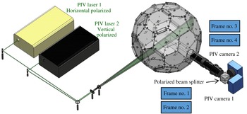
We used an in-house developed planar 4F-PTV technique for the measurement of particle-pair RV in this study, as shown in figure 1. The detail of the 4F-PTV has been described by Dou et al. (Reference Dou, Ireland, Bragg, Liang, Collins and Meng2017). Briefly, the 4F-PTV system employs two double-exposure particle image velocimetry (PIV) cameras and two double-pulse PIV lasers. The PIV systems are combined together spatially and temporally. Spatially, the two PIV laser beams are overlapped to illuminate the same flow region, and the two PIV cameras are placed orthogonally next to a polarized beam splitter to focus on the same flow region. Temporally, a timing unit synthetizes the two PIV lasers and cameras. The two PIV lasers each generate two short laser pulses, leading to four consecutively generated laser pulses with the same time interval. The first PIV camera captures the first and second particle images, while the second PIV camera captures the third and fourth particle images. Since polarized beam splitters are used and the laser pulses from the two PIV lasers are horizontally and vertically polarized, these two double exposures are not contaminated with each other. This high-speed planar 4F-PTV technique has the advantage of a very short time interval (of the order of microseconds) and accurate particle pairing capability which enables high-speed particle tracking over four consecutive frames using routine laboratory equipment (i.e. regular PIV systems).

2.2 Experimental conditions

The turbulence Taylor-microscale Reynolds number is expressed as

where $u^{\prime }$ is the turbulence strength, $\unicode[STIX]{x1D710}$ is the kinematic viscosity and $\unicode[STIX]{x1D700}$ is the turbulence kinetic energy dissipation rate. The inertia of particles in isotropic turbulence is quantified by the particle Stokes number, $St\equiv \unicode[STIX]{x1D70F}_{p}/\unicode[STIX]{x1D70F}_{\unicode[STIX]{x1D702}}$ , the ratio of the particle response time, $\unicode[STIX]{x1D70F}_{p}=\unicode[STIX]{x1D70C}_{p}d^{2}/(18\unicode[STIX]{x1D710}\unicode[STIX]{x1D70C}_{f})$ , to the turbulence Kolmogorov time scale, $\unicode[STIX]{x1D70F}_{\unicode[STIX]{x1D702}}=\sqrt{\unicode[STIX]{x1D710}/\unicode[STIX]{x1D700}}$ . It can be shown that

Here, $\unicode[STIX]{x1D70C}_{p}$ and $\unicode[STIX]{x1D70C}_{f}$ are the particle and fluid densities respectively and $d$ is the particle diameter.

Figure 1.

The set-up for measuring the inertial particle-pair RV using planar 4F-PTV in a homogeneous and isotropic turbulence chamber.

In order to generate a wide range of $St$ values at different $R_{\unicode[STIX]{x1D706}}$ values in our HIT chamber, we used two types of commercial particles: low-density glass bubbles (3M Inc., K25, $\unicode[STIX]{x1D70C}_{p}=0.25~\text{g}~\text{cm}^{-3}$ ) and high-density glass bubbles (3M Inc., S60, $\unicode[STIX]{x1D70C}_{p}=0.60~\text{g}~\text{cm}^{-3}$ ). Both the low- and the high-density glass bubbles were run through a series of sieves (ASTM E161 compliant) to generate diameter ranges (5– $10~\unicode[STIX]{x03BC}\text{m}$ , $15{-}20~\unicode[STIX]{x03BC}\text{m},25{-}32~\unicode[STIX]{x03BC}\text{m}$ , $32{-}38~\unicode[STIX]{x03BC}\text{m}$ and $38{-}45~\unicode[STIX]{x03BC}\text{m}$ ) in a particle separation instrument (GilSonic UltraSiever GA-8). 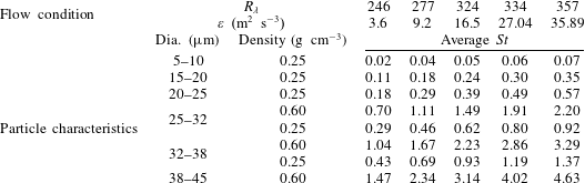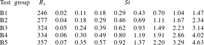Based on the available flow conditions in the fan-driven HIT chamber ( $R_{\unicode[STIX]{x1D706}}=246,277,324,334$ and 357), as well as the obtainable particle densities and diameters, we list all possible experimental conditions in table 1. It should be noted that the particle samples in the experiments were narrowly polydispersed, and the effective $St$ of a group of polydispersed particles could be slightly different from their mean $St$ (Zaichik, Simonin & Alipchenkov Reference Zaichik, Simonin and Alipchenkov2006).

Table 1.

The experimental conditions for the particle-laden turbulence in the HIT chamber used in this study. In some particle size ranges, two particle densities were required. In total, 40 unique experimental conditions were used.

2.3 Experimental design

In order to independently study the effects of $R_{\unicode[STIX]{x1D706}}$ and $St$ on particle-pair RV statistics, we conducted two series of experiments: experiment A (sweeping $R_{\unicode[STIX]{x1D706}}$ at fixed $St$ ) and experiment B (sweeping $St$ at fixed $R_{\unicode[STIX]{x1D706}}$ ). The two variables were controlled independently by changing the flow conditions and particle characteristics. To compare with the DNS results of particle-pair RV by Ireland et al. (Reference Ireland, Bragg and Collins2016a ), ideally we should match the $R_{\unicode[STIX]{x1D706}}$ and $St$ of our experiments with their DNS conditions. In practice, the available $R_{\unicode[STIX]{x1D706}}$ values for experiments are determined by the flow facility (table 1), and the whole range of experimental $R_{\unicode[STIX]{x1D706}}$ (247–357) fell between two of the $R_{\unicode[STIX]{x1D706}}$ values in the DNS by Ireland et al. (Reference Ireland, Bragg and Collins2016a ), namely 224 and 398. Since there was essentially no difference in mean inward RV, $\langle w_{r}^{-}\rangle$ , and variance of RV, $\langle w_{r}^{2}\rangle$ , under these two $R_{\unicode[STIX]{x1D706}}$ values over the range (small and intermediate $St$ and $r$ ) of interest in the DNS results (see figure 15 of Ireland et al. Reference Ireland, Bragg and Collins2016a ), we used their DNS results under $R_{\unicode[STIX]{x1D706}}=398$ and $St=0,0.05,0.3,0.5,1,2,3$ and $10$ to compare with our experimental measurements.

Experiment A: Sweeping $R_{\unicode[STIX]{x1D706}}$ at fixed $St$ . To study the effect of $R_{\unicode[STIX]{x1D706}}$ on the particle-pair RV, we experimentally swept $R_{\unicode[STIX]{x1D706}}$ at six target $St$ values, namely $St=0.05$ , 0.3, 0.5, 1, 2 and 3. In practice, it is difficult to sweep $R_{\unicode[STIX]{x1D706}}$ while keeping $St$ constant, since an increase of $R_{\unicode[STIX]{x1D706}}$ is accompanied by a decrease of $\unicode[STIX]{x1D70F}_{\unicode[STIX]{x1D702}}$ and thereby an increase of $St$ for the same particles. To maintain a nominal $St$ value, increasing $R_{\unicode[STIX]{x1D706}}$ requires decreasing particle time scale $\unicode[STIX]{x1D70F}_{p}$ accordingly. This requires either the particle diameter ( $d$ ) or the density ( $\unicode[STIX]{x1D70C}$ ) or both to be reduced accordingly as well. Since the available particle densities and diameter ranges were limited, we had to choose different particles for different $R_{\unicode[STIX]{x1D706}}$ in order to get $St$ as close to the nominal $St$ values as possible.

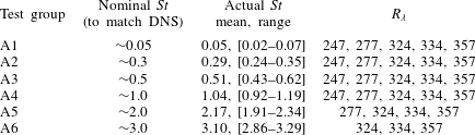
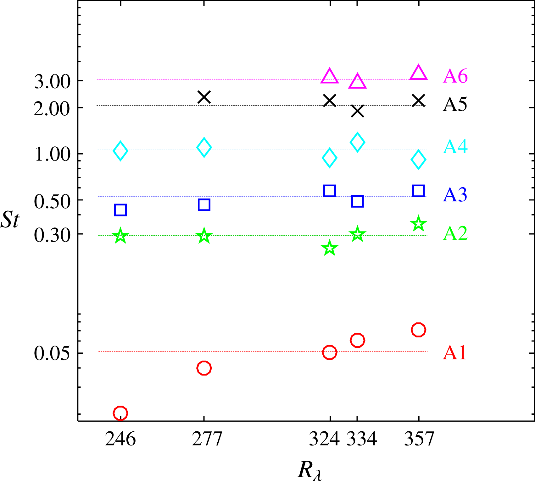
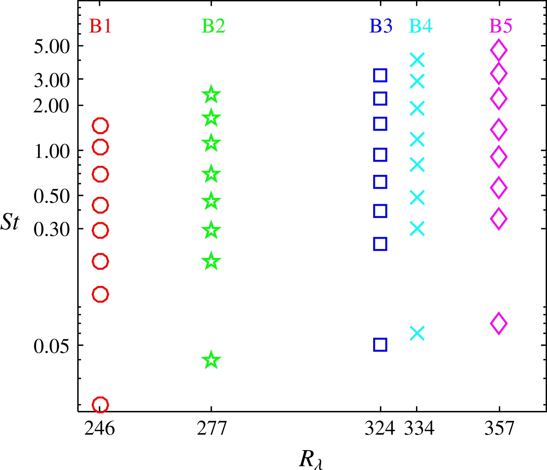
For this purpose, some of the experimental conditions in table 1 were reorganized by the nominal $St$ value, with $R_{\unicode[STIX]{x1D706}}$ being the variable, and were denoted as A1, A2, A3, A4, A5 and A6, as shown in table 2. Each test group held nominal $St$ constant while changing $R_{\unicode[STIX]{x1D706}}$ from 246 to 357. Figure 2 graphically illustrates the conditions of these test groups, showing that the fluctuations of the actual $St$ values were within 20 % of the nominal $St$ values except for test group A1.

Figure 2.

Graphical representation of table 2: experimental conditions for test groups A1–A6. Each colour represents one sweeping $R_{\unicode[STIX]{x1D706}}$ test group at a certain $St$ , while each point represents one unique experimental condition.

Table 2.

Experiment A (sweeping $R_{\unicode[STIX]{x1D706}}$ ): list of the nominal $St$ , actual $St$ and swept $R_{\unicode[STIX]{x1D706}}$ conditions for the six test groups (A1–A6).

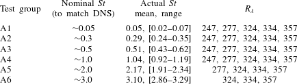
It should be noted that for $St\sim 2.0$ , the lowest $R_{\unicode[STIX]{x1D706}}$ that can be obtained is 277, and for $St\sim 3.0$ , the lowest $R_{\unicode[STIX]{x1D706}}$ that can be obtained is 324.

Experiment B: Sweeping $St$ at fixed $R_{\unicode[STIX]{x1D706}}$ . To study the effect of $St$ on the particle-pair RV, we experimentally swept $St$ at five $R_{\unicode[STIX]{x1D706}}$ values, namely $R_{\unicode[STIX]{x1D706}}=246$ , 377, 324, 334 and 357. To change $St$ at fixed $R_{\unicode[STIX]{x1D706}}$ , the flow condition was held constant and different particles were used. 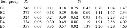For each flow condition and thus $R_{\unicode[STIX]{x1D706}}$ , all particle size and density permutations listed in table 1 were used to acquire eight $St$ values. 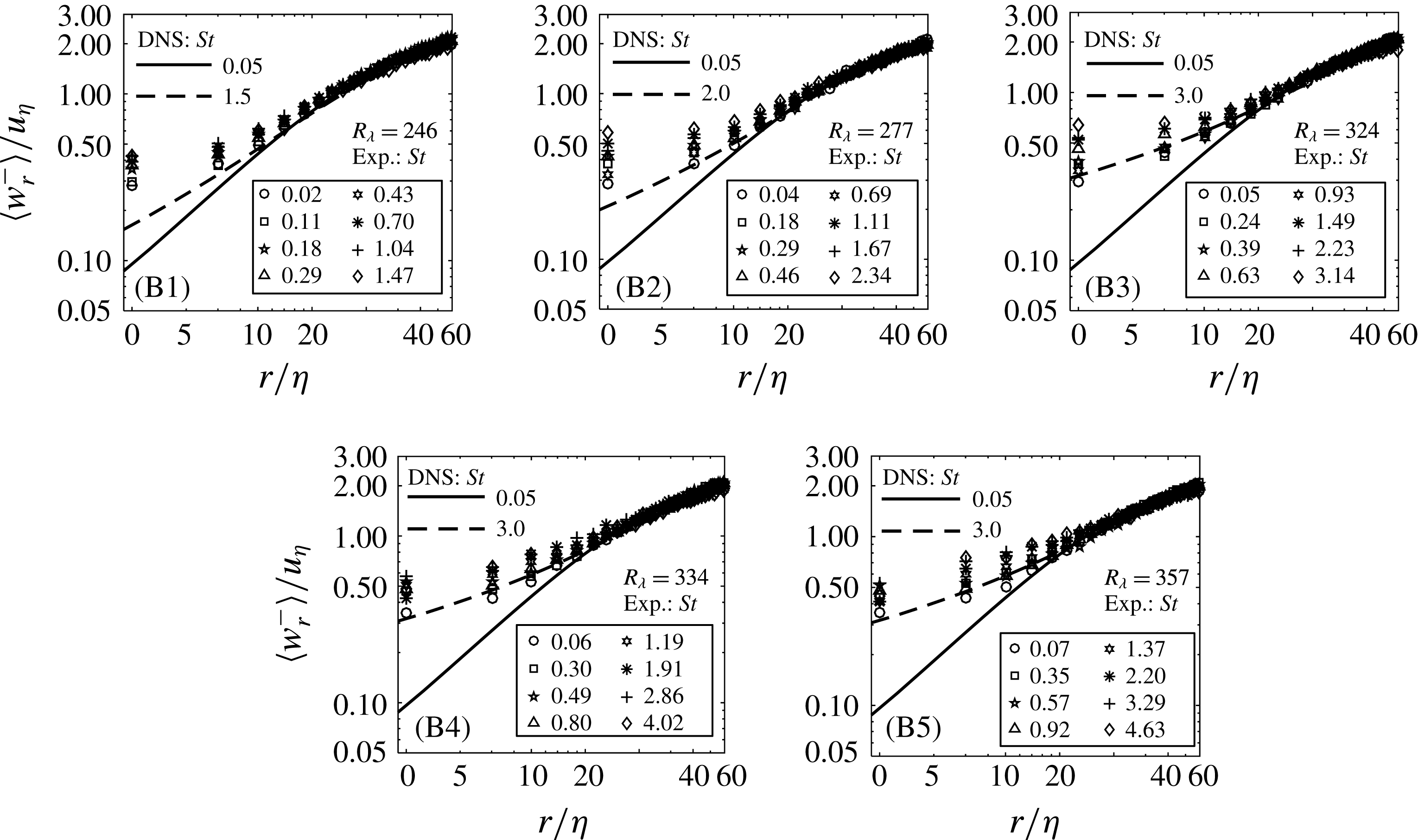The test groups for five different $R_{\unicode[STIX]{x1D706}}$ values are denoted as B1, B2, B3, B4 and B5, and are shown in table 3 and figure 3.

Figure 3.

Graphical representation of table 3: experimental conditions for test groups B1–B5. Each colour represents one sweeping $St$ test group at a certain $R_{\unicode[STIX]{x1D706}}$ , while each point represents one unique experimental condition.

2.4 Experimental procedure

For all of the 40 experimental conditions (table 1), we performed particle-pair RV measurement using the planar 4F-PTV technique in the HIT chamber. Statistics of the particle motion were only collected and computed once the turbulence had reached a statistically stationary state plus an additional 10 large-eddy time scales. Furthermore, the particle number density in the turbulence chamber was estimated to be below 50 per centimetre cubed (particle volume fraction of order $10^{-6}$ ), such that the system could be considered to be dilute. Under each test condition, we obtained 10 000 quadruple-exposure particle images in 20 runs of 500 consecutive quadruple pulses, repeated at 5–9.5 Hz. The time interval in the quadruple exposure varied between 38  $\unicode[STIX]{x03BC}\text{s}$ and 91  $\unicode[STIX]{x03BC}\text{s}$ for different values of $R_{\unicode[STIX]{x1D706}}$ . In each quadruple exposure, we obtained individual particle positions and velocities. We calculated the particle-pair RV as

where $\boldsymbol{v}_{A}$ and $\boldsymbol{v}_{B}$ are the velocity vectors of particles A and B respectively, and $\boldsymbol{r}$ is the distance vector from particle A to particle B. The calculated particle-pair RVs, $w_{r}(r)$ , were binned with the particle separation distance, $r$ , at increments of $\unicode[STIX]{x1D702}$ . Particle-pair RV statistics of mean inward particle-pair RV, $\langle w_{r}^{-}\rangle$ , and variance of particle-pair RV, $\langle w_{r}^{2}\rangle$ , were obtained over a wide range of $r$ . We calculated all experimental uncertainties following the procedure reported in appendix B of Dou et al. (Reference Dou, Ireland, Bragg, Liang, Collins and Meng2017). In the final calculation, we normalized $r$ , $\langle w_{r}^{-}\rangle$ and $\langle w_{r}^{2}\rangle$ by the Kolmogorov length scale $\unicode[STIX]{x1D702}$ , the Kolmogorov velocity scale $u_{\unicode[STIX]{x1D702}}$ and the square of the Kolmogorov velocity scale $u_{\unicode[STIX]{x1D702}}^{2}$ respectively. We then plotted these normalized quantities based on the test groups in experiments A and B.

Table 3.

Experiment B (sweeping $St$ ): list of the fixed $R_{\unicode[STIX]{x1D706}}$ and swept $St$ conditions for the five test groups (B1–B5).

2.5 Monte Carlo analysis to account for out-of-plane components of the particle-pair RV

The planar 4F-PTV technique measures the particle-pair RV within a laser light sheet that has a finite thickness of $8\unicode[STIX]{x1D702}$ . The laser thickness is required to contain a sufficient number of particles within the light sheet over the four consecutive exposures for accurate particle tracking. However, the planar PTV measures only the in-plane particle-pair separation and plane RV, omitting the out-of-plane components, which brings about uncertainty in the RV measurement when the particle separation distance is small. Dou et al. (Reference Dou, Ireland, Bragg, Liang, Collins and Meng2017) evaluated the finite laser thickness effect and showed that it causes an overestimation of the particle-pair RV at small $r$ . When the in-plane particle separation distance $r$ is larger than the laser thickness, the difference in $\langle w_{r}^{-}\rangle$ drops down to below 10 %. They further attempted to correct the omission of the out-of-plane components of the RV using Monte Carlo analysis (MCA) on their experimental data, assuming the same particle distribution in the out-of-plane direction as in the transverse directions based on isotropy. This correction procedure was able to eliminate the finite laser thickness effect on RV measurements for $r\gtrsim 5\unicode[STIX]{x1D702}$ .

We have applied the MCA correction to all of the experimental results for $\langle w_{r}^{-}\rangle$ in both experiments A and B to account for the finite laser thickness, and compared the results after and before the out-of-plane correction.

3.1 Mean inward particle-pair RV

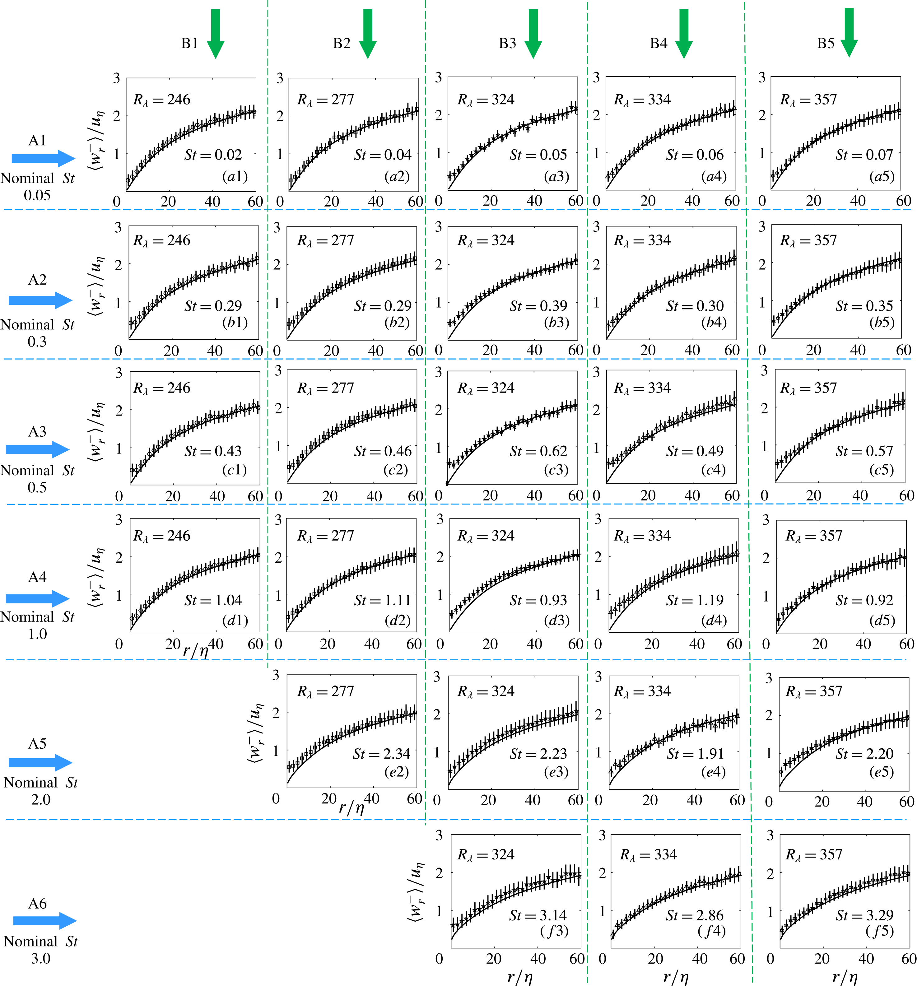
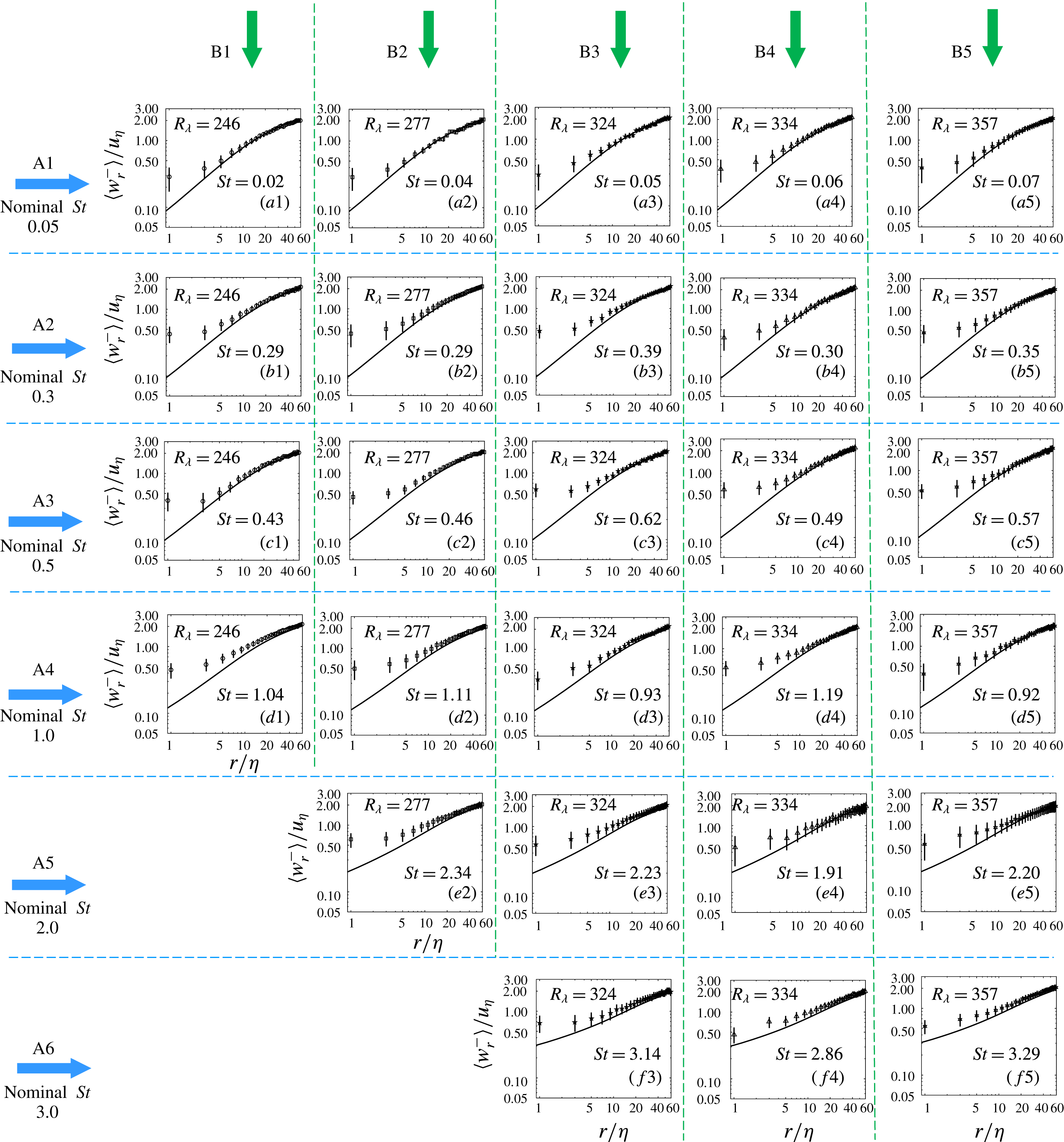
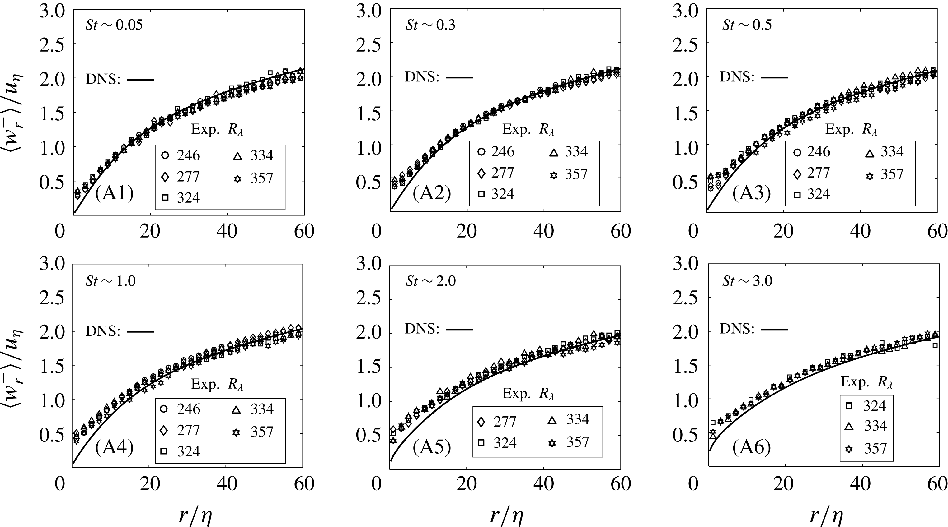
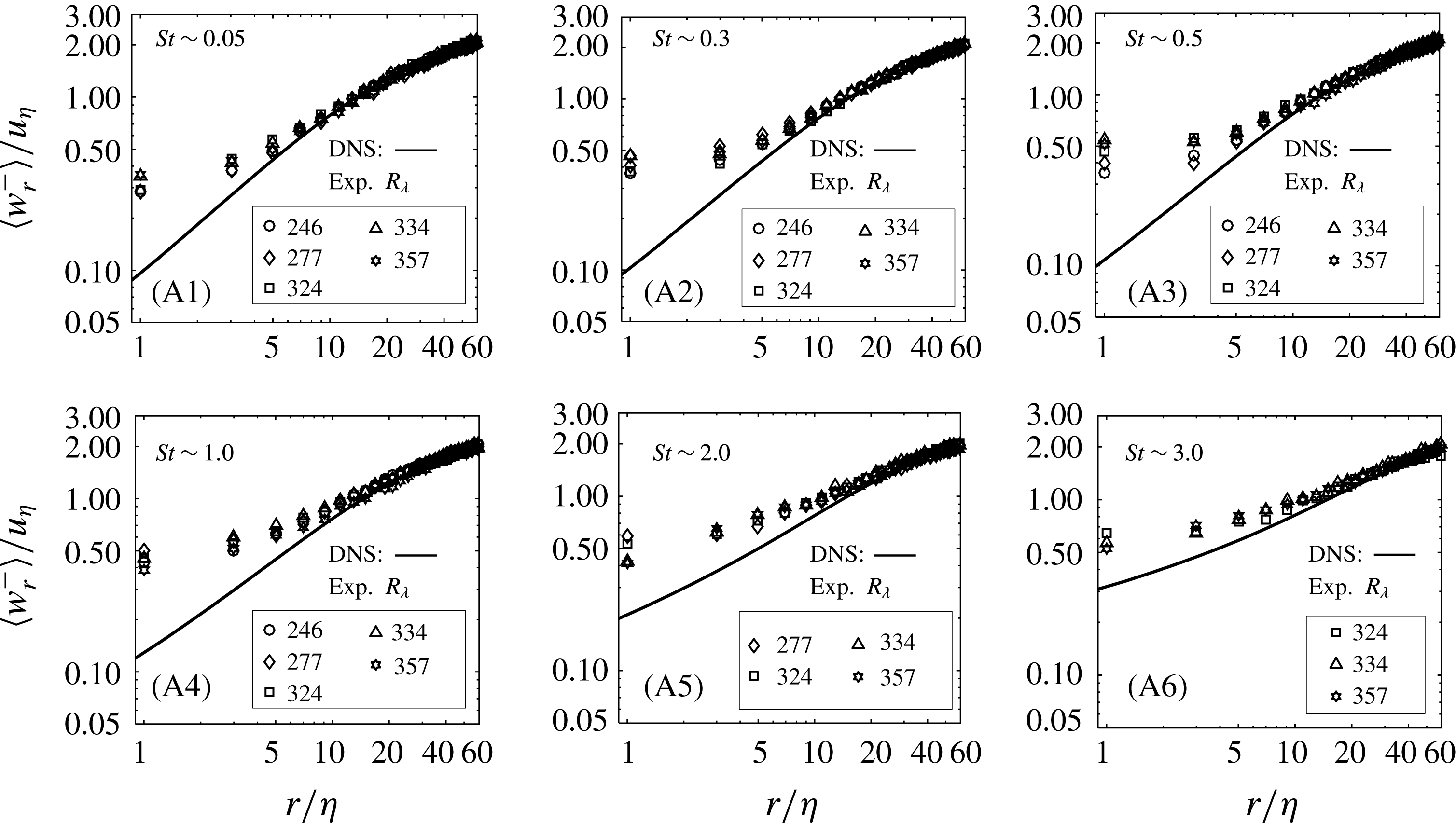
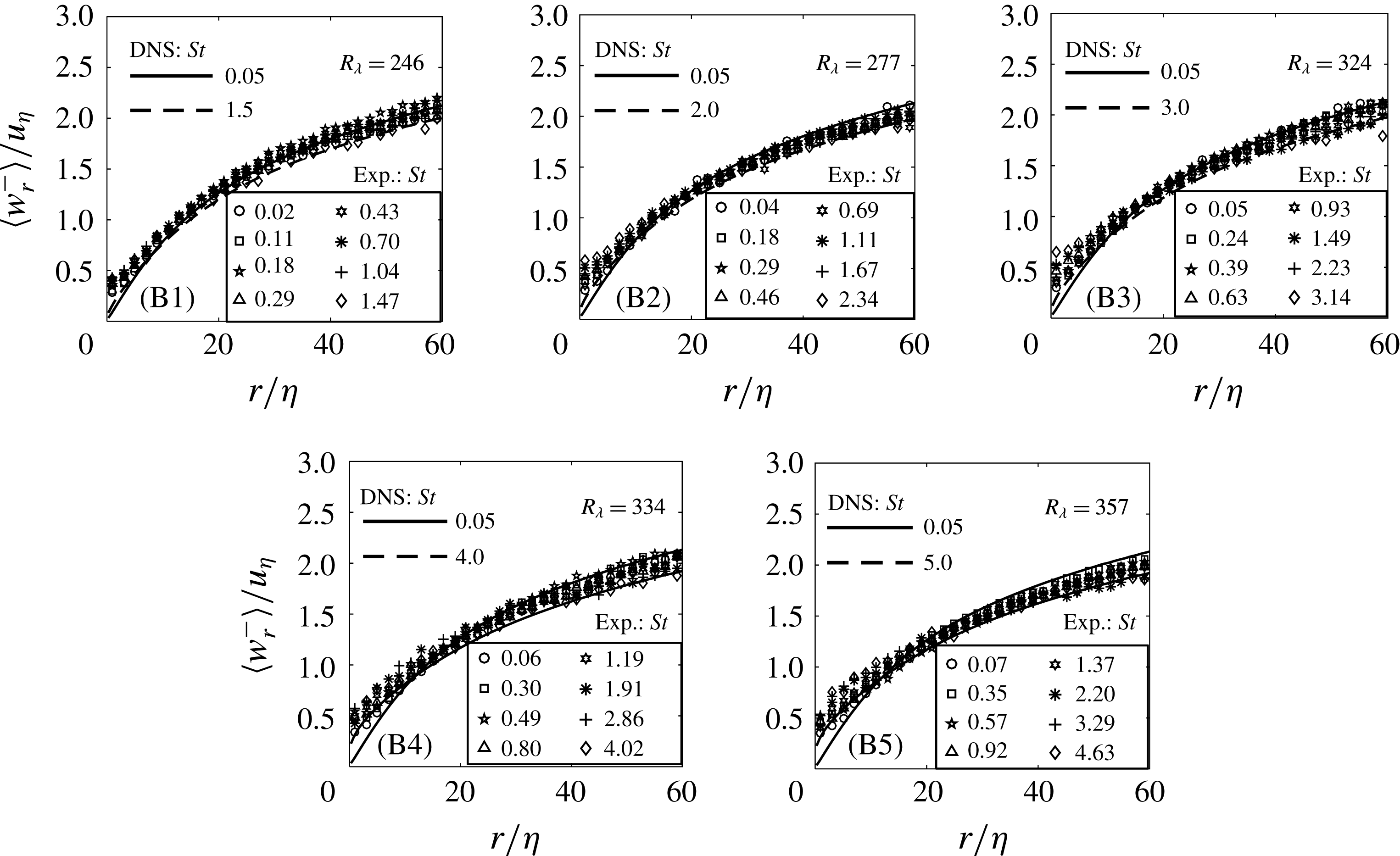
In figures 4 and 5, we plot the mean inward particle-pair RV, $\langle w_{r}^{-}\rangle$ , versus the particle-pair separation distance $r$ for some of the experimental conditions to give an overview of the general trend using both linear and log scales. The rows represent the sweeping of $R_{\unicode[STIX]{x1D706}}$ in experiment A while the columns represent the sweeping of $St$ in experiment B. Thirteen unique experimental conditions of experiment B (sweeping $St$ ) are not shown due to limited space. The DNS data from Ireland et al. (Reference Ireland, Bragg and Collins2016a ) are plotted at $St$ matching the experiment, but solely at $R_{\unicode[STIX]{x1D706}}=398.$ As stated earlier, since $\langle w_{r}^{-}\rangle$ from DNS is insensitive to $R_{\unicode[STIX]{x1D706}}$ between $R_{\unicode[STIX]{x1D706}}=88$ and 598 in the $St$ and $r$ ranges we are interested in (and, specifically, DNS results between $R_{\unicode[STIX]{x1D706}}=224$ and 398 are near-identical), DNS data at $R_{\unicode[STIX]{x1D706}}=398$ with $St$ matching experimental conditions are sufficient for comparison.

Figure 4.

The mean inward particle-pair RV $\langle w_{r}^{-}\rangle$ (normalized by the Kolmogorov velocity scale $u_{\unicode[STIX]{x1D702}}$ ) versus the particle-pair separation distance $r$ (normalized by the Kolmogorov length scale) at different values of $R_{\unicode[STIX]{x1D706}}$ and $St$ from experimental measurements (data points with error bars) and DNS (curves). The rows (A1–A6) represent the sweeping of $R_{\unicode[STIX]{x1D706}}$ in experiment A while the columns (B1–B5) represent the sweeping of $St$ in experiment B. For clarity, only 27 experimental conditions between experiments A and B are plotted, and we omit every other experimental data point in each plot. The DNS was taken from Ireland et al. (Reference Ireland, Bragg and Collins2016a ) under $R_{\unicode[STIX]{x1D706}}=398$ and the matching nominal $St$ values.

Figure 5.

Replot of figure 4 using a logarithmic scale: mean inward particle-pair RV $\langle w_{r}^{-}\rangle /u_{\unicode[STIX]{x1D702}}$ versus particle-pair separation distance $r/\unicode[STIX]{x1D702}$ at different values of $R_{\unicode[STIX]{x1D706}}$ and $St$ from experiment and DNS.

From figure 4, we notice that the experimental data for $\langle w_{r}^{-}\rangle$ versus $r$ closely match with the DNS data within the experimental uncertainty (5 % ${\sim}$ 10 %) at all experimental conditions, provided that $r\gtrsim 10\unicode[STIX]{x1D702}$ . In each case, $\langle w_{r}^{-}\rangle$ increases with decreasing slope when $r$ increases. When $r\lesssim 10\unicode[STIX]{x1D702}$ , the experimental results are consistently higher than the DNS for all experimental conditions. In order to visualize this discrepancy more clearly, we plot the same experimental conditions as those in figure 4 using logarithmic scales in figure 5. From figure 5, we see that the value of $\langle w_{r}^{-}\rangle /u_{\unicode[STIX]{x1D702}}$ in the experiment is around 0.37 (with $\pm 0.12$ fluctuations) higher than the DNS values when $r=\unicode[STIX]{x1D702}$ for all experimental conditions. This difference does not have a preferred trend when $R_{\unicode[STIX]{x1D706}}$ or $St$ is swept in experiment A or B respectively.

The persistent discrepancy between experimental and DNS results for $\langle w_{r}^{-}\rangle$ at small $r$ through all test conditions recapitulates the observation by Dou et al. (Reference Dou, Ireland, Bragg, Liang, Collins and Meng2017) at two test conditions ( $St=0.09$ and 3.46, both at $R_{\unicode[STIX]{x1D706}}=357$ ). As explained in Dou et al. (Reference Dou, Ireland, Bragg, Liang, Collins and Meng2017), particle polydispersity and finite light sheet thickness effects were the two main contributors to this discrepancy, and the contributions from these two effects were comparable. In addition, we noticed that the magnitudes of the discrepancies were very similar for all experimental conditions. This further indicates that the polydispersity and light sheet thickness effects may be the main contributors to the discrepancy, as these two effects could be approximately uniform between different test conditions, given the factor that the particle size distributions in different size ranges and light sheet thicknesses in different experimental runs were similar to each other.

3.2 Reynolds number effect on particle-pair RV

In test groups A1–A6, we are able to examine the behaviour of $\langle w_{r}^{-}\rangle$ versus $r$ as we sweep $R_{\unicode[STIX]{x1D706}}$ under similar $St$ in figure 4. To more clearly visualize any effect of the Reynolds number on $\langle w_{r}^{-}\rangle$ , we superimpose all curves of the same nominal $St$ but different $R_{\unicode[STIX]{x1D706}}$ together, and show the results in figures 6 and 7, where each plot is a combination of all plots in one row in figures 4 and 5 respectively. The DNS data at $St$ values matching the nominal $St$ values and $R_{\unicode[STIX]{x1D706}}=398$ are also plotted along with the experimental data. In general, the experimental data points do not show any systematic variation with the Reynolds number. Some of the results in figure 7 do seem to reveal a weak trend with $R_{\unicode[STIX]{x1D706}}$ at small $r$ , e.g. groups A5 and A6 in figure 7 seem to reveal a decrease in $\langle w_{r}^{-}\rangle$ as $R_{\unicode[STIX]{x1D706}}$ is increased for fixed $St$ . However, such apparent trends should be interpreted with caution since the variation with $R_{\unicode[STIX]{x1D706}}$ falls within the experimental uncertainty.

Figure 6.

Superimposition of the experimental results for all $R_{\unicode[STIX]{x1D706}}$ values under the same nominal $St$ value for test groups A1–A6. The DNS data are plotted as a solid line at an $St$ value matching the nominal $St$ value of the test group with $R_{\unicode[STIX]{x1D706}}=398$ . For clarity, we omit every other experimental data point in each plot.

Figure 7.

Replot of figure 6 using a logarithmic scale: superimposition of experimental results for all $R_{\unicode[STIX]{x1D706}}$ values under the same nominal $St$ value for test groups A1–A6.

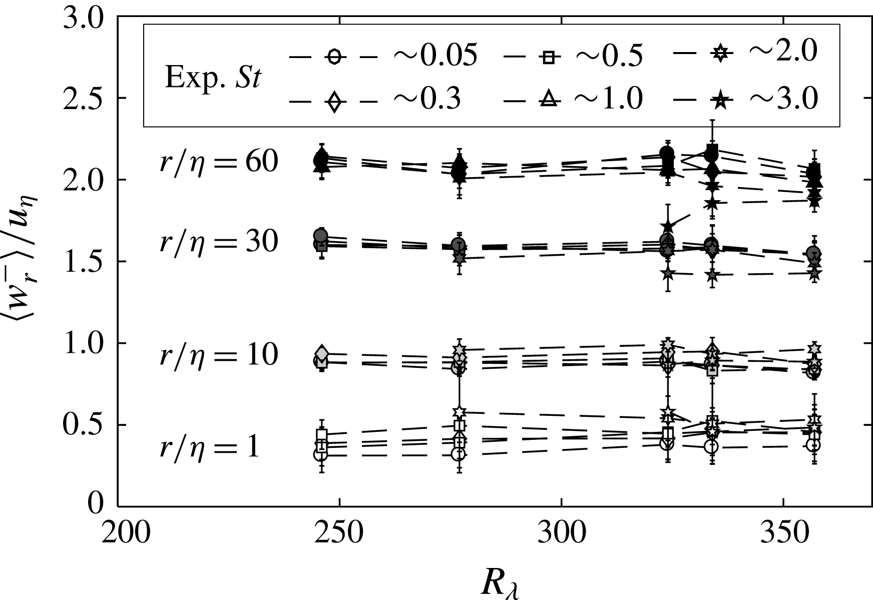
Furthermore, we plot $\langle w_{r}^{-}\rangle /u_{\unicode[STIX]{x1D702}}$ versus $R_{\unicode[STIX]{x1D706}}$ directly at four different particle separation distances ( $r=1\unicode[STIX]{x1D702},10\unicode[STIX]{x1D702},30\unicode[STIX]{x1D702}$ and $60\unicode[STIX]{x1D702}$ ) in figure 8 for all six different $St$ values. It is seen that $\langle w_{r}^{-}\rangle /u_{\unicode[STIX]{x1D702}}$ is nearly independent of $R_{\unicode[STIX]{x1D706}}$ , showing no systematic variation of $\langle w_{r}^{-}\rangle$ with increasing $R_{\unicode[STIX]{x1D706}}$ .

Figure 8.

Normalized mean inward particle-pair RV $\langle w_{r}^{-}\rangle /u_{\unicode[STIX]{x1D702}}$ against $R_{\unicode[STIX]{x1D706}}$ at four different particle separation distances, namely $r=1\unicode[STIX]{x1D702},10\unicode[STIX]{x1D702},30\unicode[STIX]{x1D702}$ and $60\unicode[STIX]{x1D702}$ . Here, $\langle w_{r}^{-}\rangle /u_{\unicode[STIX]{x1D702}}$ has no preferred change when $R_{\unicode[STIX]{x1D706}}$ increases, regardless of $St$ .

The weak Reynolds number dependence in the range of experimental observations supports previous conclusions from numerical simulations (Bec et al. Reference Bec, Biferale, Lanotte, Scagliarini and Toschi2010; Ireland et al. Reference Ireland, Bragg and Collins2016a ). Explanations for this behaviour were given in Ireland et al. (Reference Ireland, Bragg and Collins2016a ), which we now summarize. For $St\leqslant O(1)$ , the memory time scale of the inertial particles is sufficiently small such that when $r$ lies in the dissipation range, the inertial particles are only weakly affected by their memory of their interaction with the inertial range turbulence. As such, $St\leqslant O(1)$ particles are only weakly affected by the trivial Reynolds-number effect when $r$ lies in the dissipation range, whereas $St>O(1)$ particles will be affected since they retain a memory of the inertial range scales, whose properties (such as extent) strongly depend upon $R_{\unicode[STIX]{x1D706}}$ .

Outside the dissipation range, for sufficiently large $St$ , the filtering mechanism plays an important role in determining the RV behaviour. For a given $r$ , the effect of filtering depends upon the local Stokes number $St$ , and this is directly affected by the trivial $R_{\unicode[STIX]{x1D706}}$ effect (i.e. scale separation). In particular, for fixed $r$ , $St$ (and hence the filtering effect) decreases as $R_{\unicode[STIX]{x1D706}}$ is increased (fixed $\unicode[STIX]{x1D708}$ ), as observed in Ireland et al. (Reference Ireland, Bragg and Collins2016a ). This variation is not apparent in our experimental results, which is most likely because outside the dissipation range, the response times of the particles, $\unicode[STIX]{x1D70F}_{p}$ , in our experiment are too small compared with the local eddy turnover time, $\unicode[STIX]{x1D70F}_{r}$ , for the filtering mechanism to be effective (Ireland et al. (Reference Ireland, Bragg and Collins2016a ) considered particles with $St\leqslant 30$ , whereas we only have $St\leqslant 3$ in our experiment).

Concerning the non-trivial $R_{\unicode[STIX]{x1D706}}$ effect, since the low-order moments of the fluid velocity difference field are (when normalized by the Kolmogorov scales) essentially independent of $R_{\unicode[STIX]{x1D706}}$ in the dissipation range (implying that they are weakly affected by intermittency), the low-order inertial particle RV statistics are also essentially independent of $R_{\unicode[STIX]{x1D706}}$ . For the higher-order RV statistics, not investigated in this paper, this is probably not the case because of the increased intermittency of the turbulent velocity field as $R_{\unicode[STIX]{x1D706}}$ is increased.

Ireland et al. (Reference Ireland, Bragg and Collins2016a ) did detect a weak $R_{\unicode[STIX]{x1D706}}$ trend in the dissipation range low-order particle-pair RV using DNS with monodispersed particles. For example, they found a slight decrease of the mean inward particle-pair RV with $R_{\unicode[STIX]{x1D706}}$ when $St\approx O(1)$ . They attributed this to the fact that the effect of the path-history mechanism depends not only upon the value of $St$ , but also the size of the Lagrangian correlation time scales of the fluid velocity gradient measured along the inertial particle trajectories. Their DNS results showed that these time scales decrease slightly with increasing $R_{\unicode[STIX]{x1D706}}$ when $St\approx O(1)$ (a non-trivial $R_{\unicode[STIX]{x1D706}}$ effect resulting from changes to the spatiotemporal structure of the turbulence when $R_{\unicode[STIX]{x1D706}}$ is changed), which decreases the effect of the path-history mechanism, leading to the observed reduction in the RV in this regime.

The experimental uncertainty of our results in this regime (5 %–10 %) is larger than the change of $\langle w_{r}^{-}\rangle /u_{\unicode[STIX]{x1D702}}$ observed in the DNS, and as such we are not able to conclude whether or not our experiments corroborate the weak $R_{\unicode[STIX]{x1D706}}$ dependence observed in the DNS when $St\approx O(1)$ . We believe that studies on further reducing the experimental uncertainty and increasing the acquirable $R_{\unicode[STIX]{x1D706}}$ range would be very helpful to support the weak $R_{\unicode[STIX]{x1D706}}$ dependence observed in the DNS. Of course, other factors are the particle polydispersity and laser thickness effects in our experiment, which are absent in the DNS results of Ireland et al. (Reference Ireland, Bragg and Collins2016a ). How these affect the $R_{\unicode[STIX]{x1D706}}$ dependence of the inertial particle RV statistics is currently unknown, which is an important question that we intend to address in future work.

3.3 Stokes number effect on particle-pair RV

In test groups B1–B5, we are able to examine the trend of the curve of $\langle w_{r}^{-}\rangle$ versus $r$ as we sweep $St$ vertically under the same $R_{\unicode[STIX]{x1D706}}$ value in figures 4 and 5. In order to compare the curves at different $St$ values, we superimpose all curves in each test group of the same $R_{\unicode[STIX]{x1D706}}$ from experiment B and plot the vertically combined plots in figures 9 and 10 respectively. This allows us to further visualize the overall change of the curve slopes. On the combined $\langle w_{r}^{-}\rangle /u_{\unicode[STIX]{x1D702}}$ versus $r/\unicode[STIX]{x1D702}$ plot for each test group, we also plot two curves from DNS of $St$ near the upper and lower $St$ bounds of the experimental conditions for that group. Comparing the two simulation curves, and comparing between the experimental curves, we notice that the curves of $\langle w_{r}^{-}\rangle /u_{\unicode[STIX]{x1D702}}$ versus $r/\unicode[STIX]{x1D702}$ change when $St$ changes, but no obvious relationship can be obtained due the discernibility.

Figure 9.

Superimposed experimental results of all $St$ values under the same $R_{\unicode[STIX]{x1D706}}$ value for test groups B1–B5. Two DNS curves are plotted as solid and dashed lines at conditions approximating to the highest and lowest $St$ values in each test group with $R_{\unicode[STIX]{x1D706}}=398$ . For clarity, we omit every other experimental data point in each plot.

Figure 10.

Replot of figure 9 using a logarithmic scale: superimposition of experimental results of all $St$ values under the same $R_{\unicode[STIX]{x1D706}}$ value for test groups B1–B5.

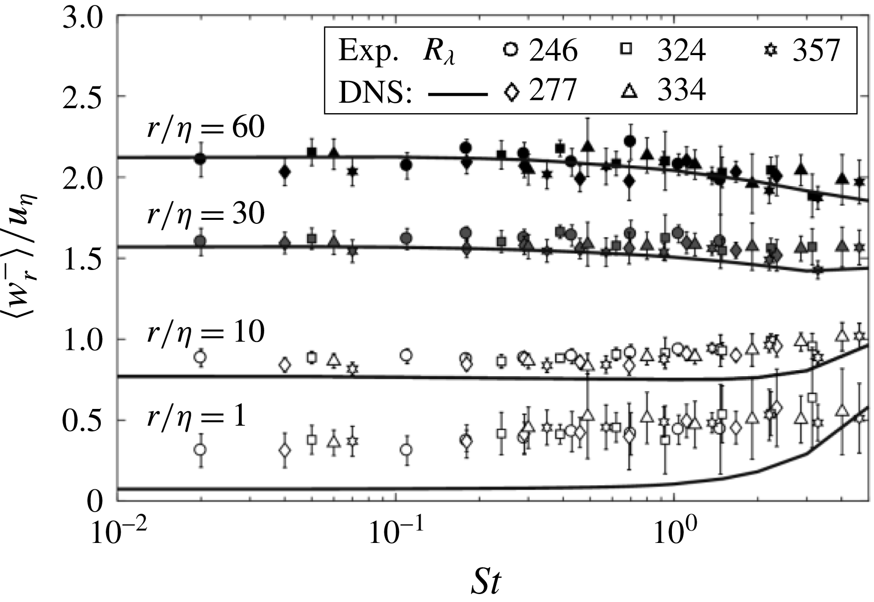
To clearly visualize this trend, we plot $\langle w_{r}^{-}\rangle /u_{\unicode[STIX]{x1D702}}$ directly against $St$ at single values of $r/\unicode[STIX]{x1D702}$ in figure 11, using experimental and DNS results. Four representative particle separation distances are shown, namely $r=1\unicode[STIX]{x1D702}$ , $10\unicode[STIX]{x1D702}$ , $30\unicode[STIX]{x1D702}$ and $60\unicode[STIX]{x1D702}$ . The experimental values are higher than the DNS values at $r=1\unicode[STIX]{x1D702}$ . When $r$ increases, the experimental and DNS results tend to agree with each other to a greater degree, and at $r=30$ and $60\unicode[STIX]{x1D702}$ , an excellent match between experiment and DNS is achieved until $St\approx 2$ . The improved agreement as $r$ is increased is probably due to the fact that the influence of the particle polydispersity and finite light sheet thickness effects becomes less important as $r$ is increased. Furthermore, both the experimental and the DNS results indicate that $\langle w_{r}^{-}\rangle$ depends more weakly upon $St$ as $r$ is increased. This is again simply a consequence of the fact that for fixed $St$ values, $\unicode[STIX]{x1D70F}_{r}$ become larger than $\unicode[STIX]{x1D70F}_{p}$ as $r$ is increased, so that the effect of inertia becomes less and less important.

Figure 11.

Normalized mean inward particle-pair RV $\langle w_{r}^{-}\rangle /u_{\unicode[STIX]{x1D702}}$ against $St$ at four different particle separation distances, namely $1\unicode[STIX]{x1D702},10\unicode[STIX]{x1D702},30\unicode[STIX]{x1D702}$ and $60\unicode[STIX]{x1D702}$ . The black lines represent the DNS results at each corresponding $r/\unicode[STIX]{x1D702}$ and $R_{\unicode[STIX]{x1D706}}=398$ . At small $r/\unicode[STIX]{x1D702}$ values, $\langle w_{r}^{-}\rangle /u_{\unicode[STIX]{x1D702}}$ increases when $St$ increases. At large $r/\unicode[STIX]{x1D702}$ values, $\langle w_{r}^{-}\rangle /u_{\unicode[STIX]{x1D702}}$ slightly decreases when $St$ increases. The value of $R_{\unicode[STIX]{x1D706}}$ does not affect the trend of the data points.

The dependence of $\langle w_{r}^{-}\rangle$ on $St$ measured from experiment is consistent with previous numerical studies (Salazar & Collins Reference Salazar and Collins2012b ; Bragg & Collins Reference Bragg and Collins2014b ) as well as the precursor of the current experimental study by Dou et al. (Reference Dou, Ireland, Bragg, Liang, Collins and Meng2017). At small $r$ , $\langle w_{r}^{-}\rangle$ increases with the particle inertia. This is because in this regime the path-history mechanism dominates. At large $r$ , the particle-pair RV decreases with increasing $St$ . This decrease is because as $r$ increases, the filtering mechanism begins to dominate over the path-history mechanism, and the filtering mechanism always reduces the RV.

3.4 Comparison between experiment, DNS and theoretical model

As discussed by Bragg & Collins (Reference Bragg and Collins2014b ), the analytical model of particle-pair RV by Pan & Padoan (Reference Pan and Padoan2010) provides a more accurate prediction of the DNS results than previous theoretical models. In order to calculate the mean inward particle-pair RV, $\langle w_{r}^{-}\rangle$ , Pan & Padoan (Reference Pan and Padoan2010) adopted the assumption that the probability distribution function (PDF) of the particle-pair RV is Gaussian, which leads to $\langle w_{r}^{-}\rangle =\sqrt{\langle w_{r}^{2}\rangle /2\unicode[STIX]{x03C0}}$ . We would like to examine this theoretical model using experimental and DNS results. This will be done in two steps: (1) a comparison of the theoretical predicted $\langle w_{r}^{2}\rangle$ and $\langle w_{r}^{-}\rangle$ with experimental and DNS results; (2) validation of the Gaussian assumption of the particle-pair RV, which underlines the relation $\langle w_{r}^{-}\rangle =\sqrt{\langle w_{r}^{2}\rangle /2\unicode[STIX]{x03C0}}$ using experimental data.

Following Pan’s theory, we first calculated $\langle w_{r}^{2}\rangle$ by solving (3.5) from Pan & Padoan (Reference Pan and Padoan2010) numerically. We then calculated $\langle w_{r}^{-}\rangle$ using the relation $\langle w_{r}^{-}\rangle =\sqrt{\langle w_{r}^{2}\rangle /2\unicode[STIX]{x03C0}}$ . These quantities were obtained at $St=[0.01-5.0]$ , $R_{\unicode[STIX]{x1D706}}=398$ and four particle separation values ( $r=1\unicode[STIX]{x1D702},10\unicode[STIX]{x1D702},30\unicode[STIX]{x1D702}$ and $60\unicode[STIX]{x1D702}$ ). 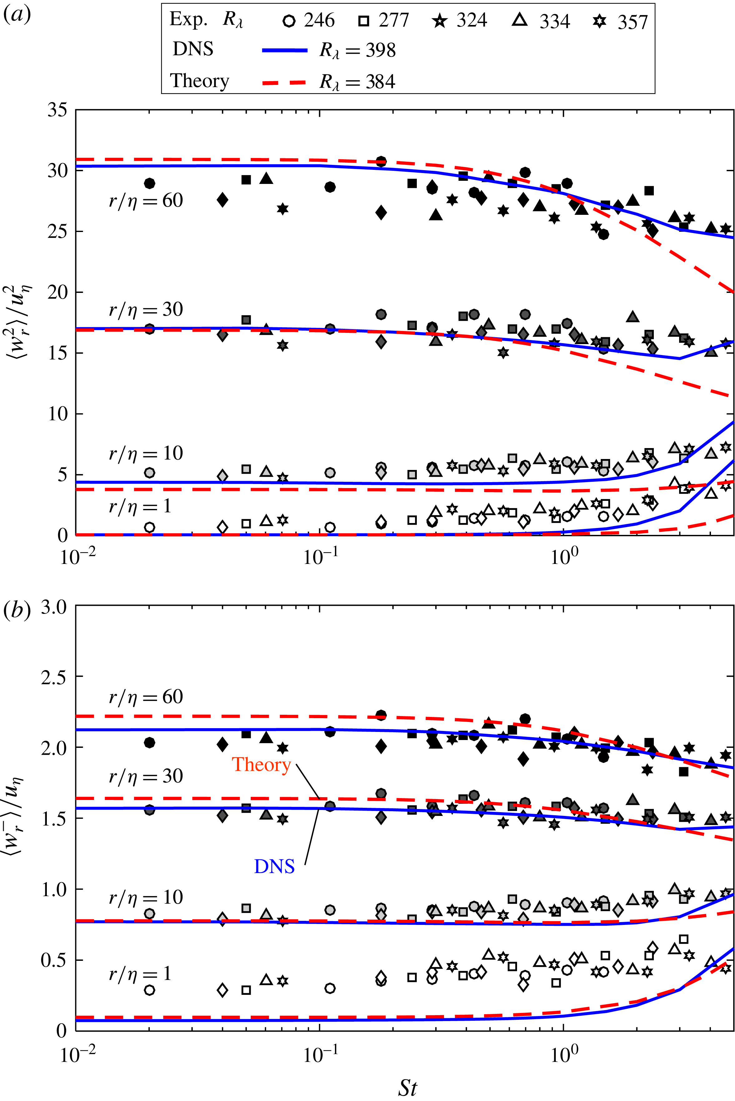We also obtained $\langle w_{r}^{2}\rangle$ versus $St$ and $\langle w_{r}^{-}\rangle$ versus $St$ at similar conditions using experimental and DNS data. Results from the theoretical, numerical and experimental calculations are normalized by the Kolmogorov velocity scale and shown in figure 12.

Figure 12.

Comparison between experimental data, simulation results and theoretical predictions of the normalized variance of the particle-pair RV and the normalized mean inward particle-pair RV versus $St$ . Here, the red lines are the theoretical model predictions, the blue curves are the DNS simulation results and the discrete dots are the experimental data. Results are plotted at particle separation distances of $r=1\unicode[STIX]{x1D702},10\unicode[STIX]{x1D702},30\unicode[STIX]{x1D702}$ and $60\unicode[STIX]{x1D702}$ . (a) Normalized variance of the particle-pair RV; (b) normalized mean inward particle-pair RV.

From figure 12, we observe that, in the range $0<St\lesssim 1.0$ , the theoretical prediction for $\langle w_{r}^{2}\rangle$ matches the DNS data well across the range of $r$ . The slight discrepancies observed are a consequence of slight errors in the empirical formula used as input to the theory for the fluid second-order structure function. Both the theoretical model and the DNS results are smaller than the experimental results at $r\lesssim 10\unicode[STIX]{x1D702}$ but match the experimental results at larger $r$ . This is again a result of particle polydispersity and finite light sheet thickness in the experiment, whose effects are only observable for $r\lesssim 10\unicode[STIX]{x1D702}$ . However, when $St\gtrsim 1.0$ , the theoretical prediction for $\langle w_{r}^{2}\rangle$ departs from both the experimental and the DNS results for all $r$ values. Indeed, the theoretical results are 20 %–100 % smaller than the DNS and experimental results.

As discussed in Bragg & Collins (Reference Bragg and Collins2014b ), a possible explanation for this disagreement is that in Pan’s theoretical model, the particle backward-in-time dispersion is approximated using its forward-in-time counterpart. The need to specify the backward-in-time dispersion arises in their model through their approximation for the fluid RVs experienced by the inertial particles along their path history. In this way, the quality of the closure they prescribe for the backward-in-time dispersion will determine, in a significant way, the degree to which their model can describe the path-history mechanism affecting the RV statistics. It was suggested in Bragg & Collins (Reference Bragg and Collins2014b ) that since inertial particles may disperse backward-in-time faster than forward-in-time, the approximation of their equivalence in the Pan theory may explain its underprediction of the particle-pair RV. In a recent study (Bragg et al. Reference Bragg, Ireland and Collins2016), it was in fact demonstrated, both theoretically and numerically, that inertial particles separate faster backward-in-time than forward-in-time, and that they may differ by orders of magnitude in the dissipation regime when $St\gtrsim O(1)$ . This then supports the explanation given by Bragg & Collins (Reference Bragg and Collins2014b ) for the cause of the underpredictions by the Pan theory.

Figure 13.

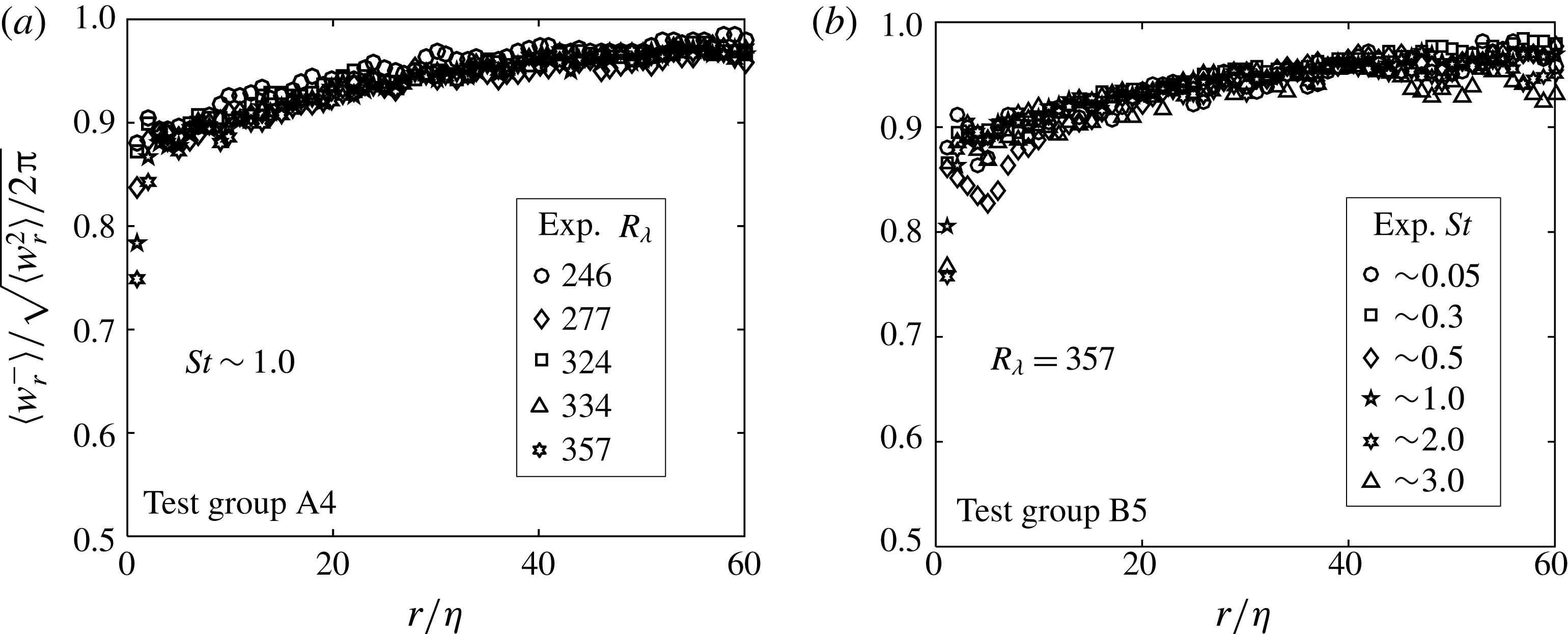
The ratio of $\langle w_{r}^{-}\rangle$ and $\sqrt{\langle w_{r}^{2}\rangle /2\unicode[STIX]{x03C0}}$ calculated from experimental data. (a) Ratio calculated from test group A4 and (b) ratio calculated from test group B5. It should be noted that regardless of the $R_{\unicode[STIX]{x1D706}}$ or $St$ , the result varies between 0.8 and 0.97 consistently.

Despite the discrepancy observed in figure 12 for $\langle w_{r}^{2}\rangle$ , the theoretical predictions for $\langle w_{r}^{-}\rangle$ compare more favourably with the DNS results. A possible explanation for this is related to the Gaussian assumption used in the theory to obtain a prediction for $\langle w_{r}^{-}\rangle$ from $\langle w_{r}^{2}\rangle$ , namely $\langle w_{r}^{-}\rangle =\sqrt{\langle w_{r}^{2}\rangle /2\unicode[STIX]{x03C0}}$ . This relationship is exact when the PDF of $w_{r}$ is Gaussian; however, we expect that this PDF will be non-Gaussian (Ireland et al. Reference Ireland, Bragg and Collins2016a ). To test the validity of $\langle w_{r}^{-}\rangle =\sqrt{\langle w_{r}^{2}\rangle /2\unicode[STIX]{x03C0}}$ , we plot the ratio $\langle w_{r}^{-}\rangle /\sqrt{\langle w_{r}^{2}\rangle /2\unicode[STIX]{x03C0}}$ as a function of $r$ from test groups A4 and B5 in figures 13(a) and 13(b) respectively. It is evident that the value of $\langle w_{r}^{-}\rangle /\sqrt{\langle w_{r}^{2}\rangle /2\unicode[STIX]{x03C0}}$ is always less than unity based on our experimental data, and it monotonically decreases with decreasing $r$ from 0.97 to 0.80. Our experiment is not able to obtain reliable data for $r<\unicode[STIX]{x1D702}$ , but the DNS results reported by Ireland et al. (Reference Ireland, Bragg and Collins2016a ) reveal that this ratio will be even lower when $r<\unicode[STIX]{x1D702}$ ( $\langle w_{r}^{-}\rangle /\sqrt{\langle w_{r}^{2}\rangle /2\unicode[STIX]{x03C0}}\approx 0.4$ when $r=0.25\unicode[STIX]{x1D702}$ ). The conclusion then is that the Gaussian result $\langle w_{r}^{-}\rangle =\sqrt{\langle w_{r}^{2}\rangle /2\unicode[STIX]{x03C0}}$ would lead to an overprediction of $\langle w_{r}^{-}\rangle$ when the correct value for $\langle w_{r}^{2}\rangle$ is prescribed, especially at small $r$ .

Therefore, although Pan’s theory underpredicts the variance $\langle w_{r}^{2}\rangle$ at $St\gtrsim 1$ , this underprediction is compensated for through its use of the Gaussian assumption to compute $\langle w_{r}^{-}\rangle$ from $\sqrt{\langle w_{r}^{2}\rangle /2\unicode[STIX]{x03C0}}$ , leading to a much better prediction for $\langle w_{r}^{-}\rangle$ than $\langle w_{r}^{2}\rangle$ when $St\gtrsim 1$ .

In addition, by improving the spatial resolution (e.g. a higher-magnification camera lens), the experimental method used in this study offers a potential for exploring the influence of $R_{\unicode[STIX]{x1D706}}$ on particle-laden flows at high $R_{\unicode[STIX]{x1D706}}$ values and large particle separations that cannot be reached by DNS in the near future.