1 Introduction
Flows of air and water like fluids are plethoric in nature as in our everyday life. They were consubstantial to the emergence of life on Earth and remain essential to its sustainability. Some involve both a liquid and gas phase, which are referred to as two-phase flows. Our everyday experience reveals that e.g. a water jet ensuing into quiescent air has strong propensity to break up into liquid fragments, subsequently atomizing into a stream of dispersed droplets in a gaseous atmosphere, called spray. Usage of sprays dates back to the Palaeolithic for painting hand stencils and they are now employed in a very wide range of situations: irrigation, cosmetics, pharmaceutics, manufacturing, decontamination. Therefore, sprays have strong implications for the economy, health, safety and well-being of modern societies.
According to Villermaux (Reference Villermaux2007), there exist three classes of theoretical elaborations for describing the atomization of liquid streams: the sequential cascade models, the aggregation models and the maximum entropy formalism. Their key benefit is to provide a plausible vision of the mechanisms of rupture and spray formation, leading to some very useful mathematical formulations for the spray drop-size distribution in the far field. The first class of elaborations dates back to Kolmogorov (Reference Kolmogorov1941b) and considers the atomization process as a successive reduction of ‘mother drops’ into a hierarchy of smaller ‘daughter drops’. This approach in its original and modern versions (Gorokhovski & Saveliev Reference Gorokhovski and Saveliev2003) thus conceptualizes the atomization process as a cascade mechanism, analogous to single fluid turbulence (Kolmogorov Reference Kolmogorov1941a), where the sense of evolution is directed towards small scales. The second class of models is due mainly to the work by Villermaux and co-workers (Marmottant & Villermaux Reference Marmottant and Villermaux2004; Villermaux, Marmottant & Duplat Reference Villermaux, Marmottant and Duplat2004). They postulated that droplets emanate from the rupture of detached ligaments which are formed during the primary atomization process. These ligaments are assumed to be virtually constituted of spherical blobs, which successively aggregate, yielding a given droplet-size distribution in the spray. Hence, the aggregation scenario indicates that the transfer among the different scales is directed towards the large scales. Finally, the last class of theory relies on the maximum entropy formalism (Sellens & Brzustowski Reference Sellens and Brzustowski1986; Dumouchel Reference Dumouchel2009). The idea is to consider, again, the liquid as being constituted of a set of elementary bricks and to compute the most probable distribution of disjoint clusters given some constraints that are imposed on the system. In the maximum entropy formalism, the process of cluster formation is done in one step and there is no explicit description of the underlying dynamics or kinematics.
It is worth mentioning that these three classes of models do not apply to the same flow regime or flow region. Indeed, the cascade model is intended to address high Weber number flow where the effect of surface tension is small compared to inertial forces. On the contrary, the aggregation scenario applies to the final stage of atomization when the break-up of liquid structures is caused by surface tension effects. Consequently, depending on the local Weber number, there could exist some zones in a flow complying more with the cascade scenario and some other regions where the aggregation process is at play. In general situations, it remains very unclear in which particular direction, if one were to exist, the evolution in scale space preferentially occurs (Herrmann & Gorokhovski Reference Herrmann and Gorokhovski2008).
All aforementioned models emphasize the cornerstone notion of constitutive scale (mother and daughter drops, blobs) and scale transfer. However, in both visions, this notion is rather ambiguous and lacks a handy, measurable definition. If a typical scale were to be unambiguously defined, it could only correspond to the diameter of a sphere (ligament) while the liquid structures are generally far from being spherical (cylindrical) in the primary or secondary atomization zone. A direct consequence is that predictions of such theories can be tested mostly in the very far field of the spray, where droplets are spherical for the ‘drop size’ to be defined and measured. Hence, they cannot be validated in the region of the flow where the processes they intend to describe are acting.
Therefore, although the cascade and the aggregation scenarios have been extremely beneficial in providing the mathematical foundations for the spray drop-size distribution, tackling the complexity and the multi-scale facets of liquid atomization requires elaborating a new observable:
(i) which applies all along the atomization process from the liquid injection to the spray dispersion, and irrespective of the flow regime,
(ii) which unambiguously defines the notion of scale thereby allowing the different mechanisms at play and the effect of some physical parameters (surface tension, density, viscosity, etc) to be scrutinized for each scale,
(iii) whose evolution can be explored in the light of a transport equation derived from first principles.
Some observables have been proposed to fulfil these requirements. First, the volume-based scale distribution (Dumouchel et al. Reference Dumouchel, Aniszewski, Vu and Ménard2017), which is the three-dimensional extension of the surface-based scale distribution (Dumouchel, Cousin & Grout Reference Dumouchel, Cousin and Grout2008) has been introduced and has shown great potential for characterizing the multi-scale facets of atomization. Another approach was proposed by Canu et al. (Reference Canu, Puggelli, Essadki, Duret, Menard, Massot, Reveillon and Demoulin2018) who defined the scale distribution on the basis of intrinsic geometrical properties of the liquid–gas interface, namely its mean and Gaussian curvatures. Recent theoretical work (Thiesset et al. Reference Thiesset, Dumouchel, Ménard, Aniszewski, Vaudor and Berlemont2019b) has shown that the volume-based scale distribution can be expressed in terms of the geometrical metrics of the liquid–gas interface (its surface area, mean and Gaussian curvatures). There thus exists a strong connection between the two latter approaches. The present work follows these lines and aims at proposing a new observable.
Besides two-phase flows, the concept of hierarchized scales among which energy is transferred has been extensively explored in the context of single-phase turbulent flows. This idea dates back to Richardson (Reference Richardson1920) and has deeply inspired von Kármán & Howarth (Reference von Kármán and Howarth1938) and Kolmogorov (Reference Kolmogorov1941a) who were the first to derive the transport equations for the two-point statistics, (i.e. correlation or structure functions) in the specific context of single-phase homogeneous isotropic turbulence. A similar framework has been followed by Yaglom (Reference Yaglom1949) who proposed the two-point statistical equation of a passive scalar field (e.g. temperature) at asymptotically high Reynolds number. Considering an analysis of the relevant metrics (e.g. velocity, temperature, concentration) not only at one point but at two points in space allows us to mathematically define the notion of scale as the straight distance between the two points considered, thereby allowing us to assess the energy budget for each scale of the turbulence spectrum. Two-point statistical equations are thus sometimes referred to as scale-by-scale budgets. A generalization of such equations to non-isotropic yet homogeneous flows was presented by Monin & Yaglom (Reference Monin and Yaglom1975) (see p. 402). In recent years, general equations for inhomogeneous anisotropic cases have been developed, see e.g. Hill (Reference Hill2002), Danaila, Antonia & Burattini (Reference Danaila, Antonia and Burattini2004) and Danaila et al. (Reference Danaila, Krawczynski, Thiesset and Renou2012). These equations are now referred to as generalized Kármán–Howarth–Kolmogorov–Monin equations. As far as the scalar field is concerned, the generalized Yaglom equation was derived by e.g. Gauding et al. (Reference Gauding, Wick, Pitsch and Peters2014) and Togni, Cimarelli & De Angelis (Reference Togni, Cimarelli and De Angelis2015).
Scale-by-scale budgets have been used extensively in recent years to characterize the statistical behaviour of some canonical flows such as grid or box turbulence (Danaila et al. Reference Danaila, Anselmet, Zhou and Antonia1999; Orlandi & Antonia Reference Orlandi and Antonia2002; Antonia & Burattini Reference Antonia and Burattini2006; Gomes-Fernandes, Ganapathisubramani & Vassilicos Reference Gomes-Fernandes, Ganapathisubramani and Vassilicos2015; Valente & Vassilicos Reference Valente and Vassilicos2015) in the presence of a mean scalar gradient (Danaila & Mydlarski Reference Danaila and Mydlarski2001; Watanabe & Gotoh Reference Watanabe and Gotoh2004), forced isotropic turbulence (Moisy, Tabeling & Willaime Reference Moisy, Tabeling and Willaime1999; Gotoh, Fukayama & Nakano Reference Gotoh, Fukayama and Nakano2002), homogeneous shear turbulence (Casciola et al. Reference Casciola, Gualtieri, Benzi and Piva2003), fully developed channel flows (Danaila et al. Reference Danaila, Anselmet, Zhou and Antonia2001; Marati, Casciola & Piva Reference Marati, Casciola and Piva2004; Saikrishnan et al. Reference Saikrishnan, De Angelis, Longmire, Marusic, Casciola and Piva2012; Cimarelli, De Angelis & Casciola Reference Cimarelli, De Angelis and Casciola2013), wall turbulence (Cimarelli et al. Reference Cimarelli, De Angelis, Schlatter, Brethouwer, Talamelli and Casciola2015), rotating turbulence (Lamriben, Cortet & Moisy Reference Lamriben, Cortet and Moisy2011; Campagne et al. Reference Campagne, Gallet, Moisy and Cortet2014), turbulent wake flows (Thiesset, Antonia & Danaila Reference Thiesset, Antonia and Danaila2013; Portela, Papadakis & Vassilicos Reference Portela, Papadakis and Vassilicos2017), round jet flows (Danaila et al. Reference Danaila, Antonia and Burattini2004; Burattini, Antonia & Danaila Reference Burattini, Antonia and Danaila2005a; Thiesset, Antonia & Djenidi Reference Thiesset, Antonia and Djenidi2014a), Rayleigh–Bénard convection (Togni et al. Reference Togni, Cimarelli and De Angelis2015) and detached turbulent flows behind a bump (Mollicone et al. Reference Mollicone, Battista, Gualtieri and Casciola2018). Scale-by-scale budgets have also been generalized to account for density variations (Lai, Charonko & Prestridge Reference Lai, Charonko and Prestridge2018), viscosity variations (Danaila, Voivenel & Varea Reference Danaila, Voivenel and Varea2017; Gauding, Danaila & Varea Reference Gauding, Danaila and Varea2018) and the modulation of small-scale statistics due to the presence of coherent structures (Thiesset, Danaila & Antonia Reference Thiesset, Danaila and Antonia2014b).
The main benefit of scale-by-scale budgets relies first on their capacity to decompose the transport of turbulent quantities in geometrical space (i.e. from one position in the flow to another) and in scale space (e.g. from large to small scales). Therefore, the effect of spatial inhomogeneity can easily be distinguished from what is commonly referred to as a cascade process or more generally a transfer in scale space. Second, it is worth stressing that such generalized two-point equations derive from first principles. They are thus exact and do not rely on particular assumptions about the flow. Third, since in large-eddy simulations (LES), the notion of scale is inherent to the filtering operation, scale energy budgets have further been shown to be useful to better characterize the energy transfer between the resolved and subgrid scales (Gualtieri et al. Reference Gualtieri, Casciola, Benzi and Piva2007; Cimarelli & De Angelis Reference Cimarelli and De Angelis2011; Cimarelli et al. Reference Cimarelli, De Angelis, Schlatter, Brethouwer, Talamelli and Casciola2015). LES models can also be developed on the basis of such a framework (Lesieur & Metais Reference Lesieur and Metais1996; Cui et al. Reference Cui, Xu, Fang, Shao and Zhang2007; Lévêque et al. Reference Lévêque, Toschi, Shao and Bertoglio2007). Finally, concomitantly with the development of two-point statistical equations, a very powerful tool based on the notion of self-similarity or self-preservation has emerged (see von Kármán & Howarth (Reference von Kármán and Howarth1938), Kolmogorov (Reference Kolmogorov1941a), George (Reference George1992a) and Antonia et al. (Reference Antonia, Smalley, Zhou, Anselmet and Danaila2003), for instance). Self-preservation states that two-point statistics can be invariant throughout their time and/or space evolutions, when normalized by an appropriate set of variables, called similarity variables. This hypothesis has led to significant contributions to the study of homogeneous isotropic turbulence (see von Kármán & Howarth (Reference von Kármán and Howarth1938), Stewart & Townsend (Reference Stewart and Townsend1951), George (Reference George1992a), Speziale & Bernard (Reference Speziale and Bernard1992) and Antonia et al. (Reference Antonia, Smalley, Zhou, Anselmet and Danaila2003), among others) and to scalar fluctuations evolving in isotropic turbulence (George Reference George1992b; Chasnov Reference Chasnov1994; Gonzalez & Fall Reference Gonzalez and Fall1998; Antonia & Orlandi Reference Antonia and Orlandi2004; Antonia et al. Reference Antonia, Smalley, Zhou, Anselmet and Danaila2004). Self-similarity has also been applied to homogeneous shear turbulence (George & Gibson Reference George and Gibson1992; Danaila et al. Reference Danaila, Antonia and Burattini2004), wake flows (Bevilaqua & Lykoudis Reference Bevilaqua and Lykoudis1978; George Reference George1989; Antonia & Mi Reference Antonia and Mi1998; Moser, Moser & Ewing Reference Moser, Moser and Ewing1998; Ewing et al. Reference Ewing, George, Rogers and Moser2007b; Thiesset et al. Reference Thiesset, Antonia and Danaila2013), turbulent jets (Bradbury Reference Bradbury1965; Antonia, Satyaprakash & Hussain Reference Antonia, Satyaprakash and Hussain1980; George Reference George1989; Burattini, Antonia & Danaila Reference Burattini, Antonia and Danaila2005b; Ewing et al. Reference Ewing, Frohnapfel, George, Pedersen and Westerweel2007a; Thiesset et al. Reference Thiesset, Antonia and Djenidi2014a) and turbulent shear layers (Bradshaw Reference Bradshaw1966; Brown & Roshko Reference Brown and Roshko1974; Fiedler Reference Fiedler1975; Hussain & Zedan Reference Hussain and Zedan1978a,Reference Hussain and Zedanb). It is important to stress that the quest for self-similar solutions has motivated many aspects of research in turbulence since it has the potential of reducing partial differential equations to ordinary differential equations leading to simple closures for the scale-by-scale budgets. In addition, when the most appropriate similarity variables are identified, this greatly helps in providing insights into the predominant mechanisms at play in the evolution of the two-point statistics.
Note that another way of assessing the scale content of a given phenomenon is by inferring the spectral Fourier components of the fluctuating field. However, this is likely to raise some issues in some cases. First, spectra can be computed only over homogeneous directions with periodic boundary conditions. This is a very stringent restriction that makes spectra inapplicable to all flow situations. Correlation or structure functions do not suffer such a limitation. Second, as discussed by notably Lucci, Ferrante & Elghobashi (Reference Lucci, Ferrante and Elghobashi2010) and also Duret et al. (Reference Duret, Luret, Reveillon, Ménard, Berlemont and Demoulin2012), two-phase flows reveal local discontinuities associated with the presence of the interface. This can result in oscillations in the large wavenumber range which corrupt the physical interpretation of energy spectra. This issue can be alleviated in Lucci et al. (Reference Lucci, Ferrante and Elghobashi2010) by considering not the Eulerian wavenumber spectrum but the Lagrangian frequency spectrum of fluid trajectories at the sacrifice that it does not emphasize the scale but the time dynamics of the flow under consideration.
In the present study, the machinery of two-point statistical analysis and self-similarity is adapted to a relevant metric of two-phase flows with the goal of exploring the scale distribution and scale energy transfer of the liquid phase. The scalar of interest is here the liquid volume fraction (Hirt & Nichols Reference Hirt and Nichols1981; Scardovelli & Zaleski Reference Scardovelli and Zaleski1999). In the long run, our objectives in deriving such a new framework is to provide insights into (i) the preferential direction (if any) and amplitude of the transfer among the different scales and flow positions during liquid atomization, and (ii) the effect of different physical parameters (surface tension, viscosity and density, inflow velocity conditions), and the range of scales over which these parameters have an influence. Only point (i) is addressed in the present work. Although this framework applies irrespective of the investigated zone within the flow and independently of the injection regime, this very first study focuses only on a turbulent two-phase flow decaying in a triply periodic box.
This paper is organized as follows. First, the scale-by-scale budget for the liquid volume fraction is presented. The derivation is given in great detail in appendices A–C, so that the reader can easily follow the different calculation steps. In this first section, we put particular emphasis on the physical interpretation of the different terms present in the equations. Then, the numerical database allowing this new framework to be appraised is presented. Specific care is given to the appropriateness of the spatial resolution and statistical convergence. Then, the two-point statistical analysis or the liquid volume fraction flow is provided. Conclusions are drawn in a last section.
2 Theoretical considerations
2.1 The liquid volume fraction function
The liquid volume fraction (abbreviated LVF and noted  $\unicode[STIX]{x1D719}$) designates the portion of liquid contained within a given volume. The LVF
 $\unicode[STIX]{x1D719}=1$ in the liquid phase and
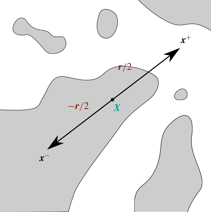
 $\unicode[STIX]{x1D719}=0$ in the gas phase. An example of such a field function is portrayed in figure 1.
Example of LVF field. Dark regions correspond to the liquid phase and white regions to the gas phase. The interface is also displayed as black curves. The two points  $\boldsymbol{x}^{+}$ and
 $\boldsymbol{x}^{-}$ used to calculate increments are also represented together with the midpoint
 $\boldsymbol{X}$ and the separation vector
 $\boldsymbol{r}$.

When the flow is incompressible with no phase change, the transport equation for the LVF reads
 $$\begin{eqnarray}\displaystyle \unicode[STIX]{x2202}_{t}\unicode[STIX]{x1D719}+\unicode[STIX]{x1D735}_{\boldsymbol{x}}\boldsymbol{\cdot }\boldsymbol{u}\unicode[STIX]{x1D719}=0, & & \displaystyle\end{eqnarray}$$
where  $\unicode[STIX]{x2202}_{t}\equiv \unicode[STIX]{x2202}/\unicode[STIX]{x2202}t$ and
 $\unicode[STIX]{x1D735}_{\boldsymbol{x}}$ is the gradient operator with respect to the coordinate
 $\boldsymbol{x}$. The equation for the LVF is therefore that of a non-diffusive passive scalar. The effect of fluid viscosity and density jumps together with surface tension of the liquid–gas interface is implicit in this equation through the roles they play in the velocity and pressure fields.
2.2 LVF transport in seven-dimensional space
The algebra for deriving the two-point equation of the liquid volume fraction is similar to what was presented in e.g. Hill (Reference Hill2002) and Danaila et al. (Reference Danaila, Antonia and Burattini2004) for the velocity field. Application to such a machinery to the LVF is detailed in appendices A to C.
A convenient form of the scale-by-scale budget is derived in appendix C and is given by
 $$\begin{eqnarray}\displaystyle & \displaystyle \unicode[STIX]{x2202}_{t}\overline{(\unicode[STIX]{x1D6FF}\unicode[STIX]{x1D719}^{\prime })^{2}}+\unicode[STIX]{x1D735}_{\boldsymbol{r}}\boldsymbol{\cdot }\overline{(\unicode[STIX]{x1D6FF}\boldsymbol{u})(\unicode[STIX]{x1D6FF}\unicode[STIX]{x1D719}^{\prime })^{2}}+2\overline{(\unicode[STIX]{x1D6FF}\unicode[STIX]{x1D719}^{\prime })(\unicode[STIX]{x1D6FF}\boldsymbol{u}^{\prime })}\boldsymbol{\cdot }\unicode[STIX]{x1D735}_{\boldsymbol{r}}(\unicode[STIX]{x1D6FF}\overline{\unicode[STIX]{x1D719}}) & \displaystyle \nonumber\\ \displaystyle & \displaystyle \quad +\unicode[STIX]{x1D735}_{\boldsymbol{X}}\boldsymbol{\cdot }\overline{(\unicode[STIX]{x1D70E}\boldsymbol{u})(\unicode[STIX]{x1D6FF}\unicode[STIX]{x1D719}^{\prime })^{2}}+2\overline{(\unicode[STIX]{x1D6FF}\unicode[STIX]{x1D719}^{\prime })(\unicode[STIX]{x1D70E}\boldsymbol{u}^{\prime })}\boldsymbol{\cdot }\unicode[STIX]{x1D735}_{\boldsymbol{X}}(\unicode[STIX]{x1D6FF}\overline{\unicode[STIX]{x1D719}})=0, & \displaystyle\end{eqnarray}$$
which can formally be written as (Mollicone et al. Reference Mollicone, Battista, Gualtieri and Casciola2018)
 $$\begin{eqnarray}\displaystyle \unicode[STIX]{x2202}_{t}\overline{(\unicode[STIX]{x1D6FF}\unicode[STIX]{x1D719}^{\prime })^{2}}+\unicode[STIX]{x1D735}_{\boldsymbol{r}}\boldsymbol{\cdot }\unicode[STIX]{x1D731}_{\boldsymbol{r}}+\unicode[STIX]{x1D735}_{\boldsymbol{X}}\boldsymbol{\cdot }\unicode[STIX]{x1D731}_{\boldsymbol{X}}=\unicode[STIX]{x1D6F1}_{\boldsymbol{r}}+\unicode[STIX]{x1D6F1}_{\boldsymbol{X}}. & & \displaystyle\end{eqnarray}$$
The quantity under consideration is here the second-order moment (or structure function) of the increment (the difference)  $\unicode[STIX]{x1D6FF}\unicode[STIX]{x1D719}^{\prime }=\unicode[STIX]{x1D719}^{\prime }(\boldsymbol{x}^{+})-\unicode[STIX]{x1D719}^{\prime }(\boldsymbol{x}^{-})$ where
 $\unicode[STIX]{x1D719}^{\prime }\equiv \unicode[STIX]{x1D719}-\overline{\unicode[STIX]{x1D719}}$ is the fluctuating component of the LVF field and the overbar denotes a suitable average;
 $\overline{(\unicode[STIX]{x1D6FF}\unicode[STIX]{x1D719}^{\prime })^{2}}$ is generally interpreted as the (cumulative) ‘energy’ content of the LVF fluctuations at a given position in the flow and at a given scale. This quantity depends a priori on time, on the position in the flow (more precisely the mid-point
 $\boldsymbol{X}$ between
 $\boldsymbol{x}^{+}$ and
 $\boldsymbol{x}^{-}$, see figure 1) and on the separation vector
 $\boldsymbol{r}=\boldsymbol{x}^{+}-\boldsymbol{x}^{-}$. In addition to a non-stationary term, equation (2.3) reveals two flux terms, in the
 $\boldsymbol{r}$- and
 $\boldsymbol{X}$-space, respectively. These are expressed as follows
 $$\begin{eqnarray}\displaystyle & \displaystyle \unicode[STIX]{x1D731}_{\boldsymbol{r}}=\overline{(\unicode[STIX]{x1D6FF}\boldsymbol{u})(\unicode[STIX]{x1D6FF}\unicode[STIX]{x1D719}^{\prime })^{2}}=(\unicode[STIX]{x1D6FF}\overline{\boldsymbol{u}})\overline{(\unicode[STIX]{x1D6FF}\unicode[STIX]{x1D719}^{\prime })^{2}}+\overline{(\unicode[STIX]{x1D6FF}\boldsymbol{u}^{\prime })(\unicode[STIX]{x1D6FF}\unicode[STIX]{x1D719}^{\prime })^{2}}, & \displaystyle\end{eqnarray}$$
 $$\begin{eqnarray}\displaystyle & \displaystyle \unicode[STIX]{x1D731}_{\boldsymbol{X}}=\overline{(\unicode[STIX]{x1D70E}\boldsymbol{u})(\unicode[STIX]{x1D6FF}\unicode[STIX]{x1D719}^{\prime })^{2}}=(\unicode[STIX]{x1D70E}\overline{\boldsymbol{u}})\overline{(\unicode[STIX]{x1D6FF}\unicode[STIX]{x1D719}^{\prime })^{2}}+\overline{(\unicode[STIX]{x1D70E}\boldsymbol{u}^{\prime })(\unicode[STIX]{x1D6FF}\unicode[STIX]{x1D719}^{\prime })^{2}}, & \displaystyle\end{eqnarray}$$
 $\unicode[STIX]{x1D70E}\unicode[STIX]{x1D6FD}=(\unicode[STIX]{x1D6FD}^{+}+\unicode[STIX]{x1D6FD}^{-})/2$;
 $\unicode[STIX]{x1D735}_{\boldsymbol{r}}$ and
 $\unicode[STIX]{x1D735}_{\boldsymbol{X}}$ denote the gradient operator with respect to the
 $\boldsymbol{r}$-space and
 $\boldsymbol{X}$-space, respectively. Therefore,
 $\unicode[STIX]{x1D735}_{\boldsymbol{r}}\boldsymbol{\cdot }\unicode[STIX]{x1D731}_{\boldsymbol{r}}$ and
 $\unicode[STIX]{x1D735}_{\boldsymbol{X}}\boldsymbol{\cdot }\unicode[STIX]{x1D731}_{\boldsymbol{X}}$ are characteristics of a transfer in the
 $\boldsymbol{r}$-space and
 $\boldsymbol{X}$-space, respectively. As per Valente & Vassilicos (Reference Valente and Vassilicos2015) and Gomes-Fernandes et al. (Reference Gomes-Fernandes, Ganapathisubramani and Vassilicos2015), the term
 $\unicode[STIX]{x1D731}_{\boldsymbol{r}}$ represents the flux of the fluctuating quantity
 $(\unicode[STIX]{x1D6FF}\unicode[STIX]{x1D719}^{\prime })^{2}$ from spherical shells centred at
 $\boldsymbol{X}$ with radius
 $r=|\boldsymbol{r}|$ to spherical shells centred at the same
 $\boldsymbol{X}$ but with a different radius or within the same spherical shell but with a different orientation
 $\boldsymbol{r}/r$. This flux operates with a characteristic velocity
 $\unicode[STIX]{x1D6FF}\boldsymbol{u}=\unicode[STIX]{x1D6FF}\overline{\boldsymbol{u}}+\unicode[STIX]{x1D6FF}\boldsymbol{u}^{\prime }$, i.e. the sum of mean and fluctuating velocity increments. On the other hand, the term
 $\unicode[STIX]{x1D731}_{\boldsymbol{X}}$ represents the flux of the fluctuating quantity
 $(\unicode[STIX]{x1D6FF}\unicode[STIX]{x1D719}^{\prime })^{2}$ from spherical shells centred at
 $\boldsymbol{X}$ with radius
 $r=|\boldsymbol{r}|$ to a spherical shell of same radius centred at another point in flow–position space. The latter is driven by a characteristic velocity
 $\unicode[STIX]{x1D70E}\boldsymbol{u}=\unicode[STIX]{x1D70E}\overline{\boldsymbol{u}}+\unicode[STIX]{x1D70E}\boldsymbol{u}^{\prime }$, i.e. the sum of mean and fluctuating velocity half-sum. The right-hand side of (2.3) further contains two terms which are interpreted as some production terms due to the gradients of mean quantities in the
 $\boldsymbol{r}$-space and
 $\boldsymbol{X}$-space, respectively
 $$\begin{eqnarray}\displaystyle & \displaystyle \unicode[STIX]{x1D6F1}_{\boldsymbol{r}}=-2\overline{(\unicode[STIX]{x1D6FF}\boldsymbol{u}^{\prime })(\unicode[STIX]{x1D6FF}\unicode[STIX]{x1D719}^{\prime })}\boldsymbol{\cdot }\unicode[STIX]{x1D735}_{\boldsymbol{r}}(\unicode[STIX]{x1D6FF}\overline{\unicode[STIX]{x1D719}}), & \displaystyle\end{eqnarray}$$
 $$\begin{eqnarray}\displaystyle & \displaystyle \unicode[STIX]{x1D6F1}_{\boldsymbol{X}}=-2\overline{(\unicode[STIX]{x1D70E}\boldsymbol{u}^{\prime })(\unicode[STIX]{x1D6FF}\unicode[STIX]{x1D719}^{\prime })}\boldsymbol{\cdot }\unicode[STIX]{x1D735}_{\boldsymbol{X}}(\unicode[STIX]{x1D6FF}\overline{\unicode[STIX]{x1D719}}), & \displaystyle\end{eqnarray}$$
 $\unicode[STIX]{x1D6F1}_{\boldsymbol{r}}$ and
 $\unicode[STIX]{x1D6F1}_{\boldsymbol{X}}$ can further be seen as representative of the ‘energy’ transfer between the mean and fluctuating fields (see appendix C).
Equation (2.3) reveals that  $\overline{(\unicode[STIX]{x1D6FF}\unicode[STIX]{x1D719}^{\prime })^{2}}$ changes in time due to (i) a production mechanism associated with statistical inhomogeneity of mean quantities, and (ii) redistribution through fluxes in both scale space
 $\boldsymbol{r}$ and position space
 $\boldsymbol{X}$. Contrary to the well-known equation for the scalar field such as temperature or pollutant concentration (i.e. the generalized Yaglom equation, see e.g. Danaila et al. (Reference Danaila, Anselmet, Zhou and Antonia1999), Gauding et al. (Reference Gauding, Wick, Pitsch and Peters2014) and Togni et al. (Reference Togni, Cimarelli and De Angelis2015)), the LVF field is a non-diffusive scalar. Therefore, the diffusion term and the scalar dissipation rate do not appear in (2.3). This is a very noticeable peculiarity of the LVF, since it suggests that there is no dissipation mechanism of fluctuations of the liquid volume fraction.
2.3 Local and non-local interactions
As per Mollicone et al. (Reference Mollicone, Battista, Gualtieri and Casciola2018), it is convenient to introduce the flux convection velocities in either the  $\boldsymbol{r}$- or
 $\boldsymbol{X}$-space
 $$\begin{eqnarray}\displaystyle & \displaystyle \boldsymbol{w}_{\boldsymbol{r}}=\frac{\overline{(\unicode[STIX]{x1D6FF}\boldsymbol{u})(\unicode[STIX]{x1D6FF}\unicode[STIX]{x1D719}^{\prime })^{2}}}{\overline{(\unicode[STIX]{x1D6FF}\unicode[STIX]{x1D719}^{\prime })^{2}}}, & \displaystyle\end{eqnarray}$$
 $$\begin{eqnarray}\displaystyle & \displaystyle \boldsymbol{w}_{\boldsymbol{X}}=\frac{\overline{(\unicode[STIX]{x1D70E}\boldsymbol{u})(\unicode[STIX]{x1D6FF}\unicode[STIX]{x1D719}^{\prime })^{2}}}{\overline{(\unicode[STIX]{x1D6FF}\unicode[STIX]{x1D719}^{\prime })^{2}}} & \displaystyle\end{eqnarray}$$
 $\boldsymbol{m}$ as either
 $\boldsymbol{r}$ or
 $\boldsymbol{X}$, so that
 $\boldsymbol{w}_{\boldsymbol{m}}$ denotes either
 $\boldsymbol{w}_{\boldsymbol{r}}$ or
 $\boldsymbol{w}_{\boldsymbol{X}}$, which then allows us to write (2.3) in a Lagrangian form, viz.
 $$\begin{eqnarray}\displaystyle \unicode[STIX]{x2202}_{t}\overline{(\unicode[STIX]{x1D6FF}\unicode[STIX]{x1D719}^{\prime })^{2}}+\boldsymbol{w}_{\boldsymbol{m}}\boldsymbol{\cdot }\unicode[STIX]{x1D735}_{\boldsymbol{m}}\overline{(\unicode[STIX]{x1D6FF}\unicode[STIX]{x1D719}^{\prime })^{2}}=\unicode[STIX]{x1D6F1}_{\boldsymbol{m}}-\overline{(\unicode[STIX]{x1D6FF}\unicode[STIX]{x1D719}^{\prime })^{2}}\unicode[STIX]{x1D735}_{\boldsymbol{m}}\boldsymbol{\cdot }\boldsymbol{w}_{\boldsymbol{m}}. & & \displaystyle\end{eqnarray}$$
Note that (2.7) is not equivalent to (2.3) except if the  $\boldsymbol{X}$ and
 $\boldsymbol{r}$ spaces are independent. In case of statistically homogeneous flows (which will be the case hereafter), gradients with respect to
 $\boldsymbol{X}$ are zero and (2.7) applies and is equivalent to (2.3). The main advantage of writing the scale-by-scale budget in the form provided by (2.7) is that the transfer term is decomposed into a transport term (i.e. the rightmost term on left-hand side of (2.7)) with convection velocity
 $\boldsymbol{w}_{\boldsymbol{m}}$ whose sign indicates the direction of the flux (negative/positive when directed towards smaller/larger scales), and a sink/source term accounting for the non-solenoidal character of
 $\boldsymbol{w}_{\boldsymbol{m}}$ (the right-hand side of (2.7)). Variations of
 $\overline{(\unicode[STIX]{x1D6FF}\unicode[STIX]{x1D719}^{\prime })^{2}}$ along the trajectories of the field
 $\boldsymbol{w}_{\boldsymbol{m}}$ then appear to be due to the combined effect of production
 $\unicode[STIX]{x1D6F1}_{\boldsymbol{m}}$ and source terms associated with the non-solenoidal character of
 $\boldsymbol{w}_{\boldsymbol{m}}$.
To further elaborate on the origin of the source term  $\overline{(\unicode[STIX]{x1D6FF}\unicode[STIX]{x1D719}^{\prime })^{2}}\unicode[STIX]{x1D735}_{\boldsymbol{m}}\boldsymbol{\cdot }\boldsymbol{w}_{\boldsymbol{m}}$, it is worth applying a Helmholtz decomposition to
 $\boldsymbol{w}_{\boldsymbol{m}}$ denoting either
 $\boldsymbol{w}_{\boldsymbol{r}}$ or
 $\boldsymbol{w}_{\boldsymbol{X}}$. The velocity
 $\boldsymbol{w}_{\boldsymbol{m}}$ can then be decomposed as the sum of a divergence-free (solenoidal) and a curl-free (irrotational) component. This is written as
 $$\begin{eqnarray}\displaystyle \boldsymbol{w}_{\boldsymbol{m}}=-\unicode[STIX]{x1D735}_{\boldsymbol{m}}P_{\boldsymbol{m}}+\unicode[STIX]{x1D735}_{\boldsymbol{m}}\wedge \boldsymbol{A}_{\boldsymbol{m}}, & & \displaystyle\end{eqnarray}$$
where  $P_{\boldsymbol{m}}$ and
 $\boldsymbol{A}_{\boldsymbol{m}}$ are the scalar and vector potentials, respectively in either the
 $\boldsymbol{r}$ or
 $\boldsymbol{X}$ space. The source term
 $f_{\boldsymbol{m}}=\unicode[STIX]{x1D735}_{\boldsymbol{m}}\boldsymbol{\cdot }\boldsymbol{w}_{\boldsymbol{m}}$ can thus be expressed in the form of a Poisson equation, viz.
 $\unicode[STIX]{x1D735}_{\boldsymbol{m}}\boldsymbol{\cdot }\boldsymbol{w}_{\boldsymbol{m}}=-\unicode[STIX]{x1D735}_{\boldsymbol{m}}\boldsymbol{\cdot }(\unicode[STIX]{x1D735}_{\boldsymbol{m}}P_{m})$ with
 $\boldsymbol{m}=\boldsymbol{r}\text{ or }\boldsymbol{X}$. Using Green’s function for Poisson’s equation on an unbounded space and assuming that
 $f_{\boldsymbol{m}}$ decays faster than
 $|\boldsymbol{m}|^{-1}$ at large
 $\boldsymbol{m}$, the solution for the scalar potential is given by
 $$\begin{eqnarray}\displaystyle P_{\boldsymbol{m}}=\int _{\boldsymbol{m}^{\prime }}G_{m}(\boldsymbol{m}^{\prime }-\boldsymbol{m})f_{\boldsymbol{m}}(\boldsymbol{m}^{\prime })\,\text{d}\boldsymbol{m}^{\prime }. & & \displaystyle\end{eqnarray}$$
 $G_{m}(\boldsymbol{m}^{\prime }-\boldsymbol{m})=\{4\unicode[STIX]{x03C0}|\boldsymbol{m}^{\prime }-\boldsymbol{m}|\}^{-1}$, the Newtonian potential, describes the response of the system at a position
 $\boldsymbol{m}$ in the manifold
 $\boldsymbol{m}=\boldsymbol{r}\text{ or }\boldsymbol{X}$ to a point source located at a position
 $\boldsymbol{m}^{\prime }$. Writing the sink/source term in the form of a Poisson equation therefore suggests that a given scale (or position) interacts with all other scales (positions) through a scalar potential field. The sink/source term in (2.7) therefore contains information about the non-local character of the interactions between different scales or positions. A similar reasoning was elaborated as regards to the non-local effect of pressure in incompressible turbulence by e.g. Tsinober (Reference Tsinober2009), see p. 28. In other words, equation (2.7) can be seen as a way of decomposing the transfer terms into local and non-local processes. The rightmost term on the left-hand side of (2.7) characterizes local interactions between two neighbouring scales
 $\boldsymbol{r}$ or positions
 $\boldsymbol{X}$. Such interactions act through a local transport process. On the other hand, the rightmost term on the right-hand side of (2.7) emphasizes that there exists a potential field
 $P_{\boldsymbol{m}}$ which allows separated scales (or positions) to interact.
2.4 Further comments
It is worth recalling that (2.7) is exact (no assumptions were invoked except (2.1), see appendix A). It applies to the entire flow field, from the injection to the spray dispersion zone and irrespective of the flow configuration or regime, as long as the flow remains incompressible with no phase change. The notion of scale is explicit and unambiguously defined as the straight distance between the two points considered. Consequently, it allows us to explore notably the direction and amplitude of the transfer among the different scales, the effect of different physical parameters (surface tension, viscosity and density, inflow velocity conditions) and the range of scales over which these parameters have an influence. Consequently, transposing the two-point statistical analysis to  $\unicode[STIX]{x1D719}$ appears particularly promising for providing insights into the complex physics of liquid transport and atomization.
However, equation (2.3) or (2.7) have argument list  $(\boldsymbol{X},\boldsymbol{r},t)$, i.e. a 6 +1 dimensional problem. This is the price to pay for the transport of liquid to be explored along the geometrical and scale space. For instance, this makes its graphical representation particularly tenuous, and one generally discusses the contribution of the different terms of (2.3) or (2.7) on some submanifolds (see Mollicone et al. (Reference Mollicone, Battista, Gualtieri and Casciola2018), and references therein). This complexity can however be reduced given the possible symmetries of the problem and the averaging operators which are used. For instance, statistical homogeneity in a particular direction will cancel out the
 $\boldsymbol{X}$ gradient in this direction. Isotropy, i.e. invariance by rotation of the
 $\boldsymbol{r}$ separation vector, will allow us to write equations as a function of the separation modulus
 $r=|\boldsymbol{r}|$ only. Note also that this framework is only an exploratory tool, but is incapable of the predictions the sequential cascade (Kolmogorov Reference Kolmogorov1941a; Gorokhovski & Saveliev Reference Gorokhovski and Saveliev2003), the aggregation (Marmottant & Villermaux Reference Marmottant and Villermaux2004; Villermaux et al. Reference Villermaux, Marmottant and Duplat2004) and the maximum entropy (Sellens & Brzustowski Reference Sellens and Brzustowski1986; Dumouchel Reference Dumouchel2009) phenomenologies can provide. The reason is that (2.3) is not closed, i.e. the transport of second-order statistics depends on higher (third-) order terms.
3 Numerical database description
3.1 Numerical set-up
The theory is appraised using direct numerical simulations (DNS). We use the high-performance computing code ARCHER developed at the CORIA laboratory. It was one of the first codes worldwide to undertake the simulation of liquid-jet atomization under a realistic diesel injection configuration (Ménard, Tanguy & Berlemont Reference Ménard, Tanguy and Berlemont2007). It solves on a Cartesian mesh the one-fluid formulation of the incompressible Navier–Stokes equation, viz.
 $$\begin{eqnarray}\displaystyle \unicode[STIX]{x2202}_{t}~\unicode[STIX]{x1D70C}\boldsymbol{u}+\unicode[STIX]{x1D735}\boldsymbol{\cdot }(\unicode[STIX]{x1D70C}\boldsymbol{u}\otimes \boldsymbol{u})=-\unicode[STIX]{x1D735}p+\unicode[STIX]{x1D735}\boldsymbol{\cdot }(2\unicode[STIX]{x1D707}\unicode[STIX]{x1D63F})+\boldsymbol{f}+\unicode[STIX]{x1D6FE}\unicode[STIX]{x1D705}\unicode[STIX]{x1D6FF}_{s}\boldsymbol{n}, & & \displaystyle\end{eqnarray}$$
where  $p$ is the pressure field,
 $\unicode[STIX]{x1D63F}$ the strain rate tensor,
 $\boldsymbol{f}$ a source term,
 $\unicode[STIX]{x1D707}$ the dynamic viscosity,
 $\unicode[STIX]{x1D70C}$ the density,
 $\unicode[STIX]{x1D6FE}$ the surface tension,
 $\boldsymbol{n}$ the unit normal vector to the liquid–gas interface,
 $\unicode[STIX]{x1D705}$ its mean curvature and
 $\unicode[STIX]{x1D6FF}_{s}$ is the Dirac function characterizing the locations of the liquid–gas interface. To solve (3.1), the convective term is written in conservative form and solved using the improved Rudman (Reference Rudman1998) technique presented in Vaudor et al. (Reference Vaudor, Ménard, Aniszewski, Doring and Berlemont2017). The latter allows mass and momentum to be transported in a consistent manner, thereby enabling flows with large liquid/gas density ratios to be simulated accurately. The viscosity term is computed following the method presented by Sussman et al. (Reference Sussman, Smith, Hussaini, Ohta and Zhi-Wei2007). To ensure incompressibility of the velocity field, a Poisson equation is solved. The latter accounts for the surface tension force and is solved using a multigrid preconditioned conjugate gradient algorithm (Zhang Reference Zhang1996) coupled with a ghost-fluid method (Fedkiw et al. Reference Fedkiw, Aslam, Merriman and Osher1999).
To transport the interface, use is made of a coupled level-set and volume-of-fluid solver, in which the level-set function accurately describes the geometric features of the interface (its normal and curvature) and the volume-of-fluid function ensures mass conservation. The density is calculated from the volume-of-fluid (or liquid volume fraction) as  $\unicode[STIX]{x1D70C}=\unicode[STIX]{x1D70C}_{L}\unicode[STIX]{x1D719}+\unicode[STIX]{x1D70C}_{G}(1-\unicode[STIX]{x1D719})$, where
 $\unicode[STIX]{x1D70C}_{L},\unicode[STIX]{x1D70C}_{G}$ are the densities of the liquid and gas phase. The dynamic viscosity (
 $\unicode[STIX]{x1D707}_{L}$ or
 $\unicode[STIX]{x1D707}_{G}$) depends on the sign of the level-set function. In cells containing both a liquid and gas phase, a specific treatment is performed to evaluate the dynamic viscosity, following the procedure of Sussman et al. (Reference Sussman, Smith, Hussaini, Ohta and Zhi-Wei2007). For more information about the ARCHER solver, the reader can refer to e.g. Ménard et al. (Reference Ménard, Tanguy and Berlemont2007), Duret et al. (Reference Duret, Luret, Reveillon, Ménard, Berlemont and Demoulin2012) and Vaudor et al. (Reference Vaudor, Ménard, Aniszewski, Doring and Berlemont2017).
The simulated configuration is that of a turbulent two-phase flow in a triply periodic box similar to Duret et al. (Reference Duret, Luret, Reveillon, Ménard, Berlemont and Demoulin2012, Reference Duret, Reveillon, Menard and Demoulin2013). This academic configuration, widely explored in the context of single-phase flows, is here extended to a two-phase case. It has already proved to be extremely beneficial for better characterizing some features of primary atomization. In the particular context of two-point statistics, this configuration was chosen because it is statistically homogeneous thereby allowing us to explore the dynamics of liquid transport in scale space only.
The physical parameters are the same as Duret et al. (Reference Duret, Luret, Reveillon, Ménard, Berlemont and Demoulin2012, Reference Duret, Reveillon, Menard and Demoulin2013): the densities of liquid and gas phases are set to  $\unicode[STIX]{x1D70C}_{L}=753~\text{kg}~\text{m}^{-3}$ and
 $\unicode[STIX]{x1D70C}_{G}=25~\text{kg}~\text{m}^{-3}$, respectively, leading to a density ratio of approximately 30. The dynamic viscosities for the liquid and gas phases are
 $\unicode[STIX]{x1D707}_{L}=5.65\times 10^{-4}~\text{Pa}~\text{s}$ and
 $\unicode[STIX]{x1D707}_{G}=1.879\times 10^{-5}~\text{Pa}~\text{s}$ respectively. Therefore, the kinematic viscosity is the same for both the liquid and gas phases. The surface tension is
 $\unicode[STIX]{x1D6FE}=0.0135~\text{N}~\text{m}^{-1}$ and the box is filled with
 $\unicode[STIX]{x1D719}_{0}=10\,\%$ of liquid. The domain is
 $L=1.5\times 10^{-4}$ m wide in each direction and 2563 grid points are used for discretization. Several validation tests for the appropriateness of this resolution were undertaken by Duret et al. (Reference Duret, Luret, Reveillon, Ménard, Berlemont and Demoulin2012, Reference Duret, Reveillon, Menard and Demoulin2013) and will be further discussed below.
The actual initialization of such flow is somehow arbitrary. Possible options are to simulate an actual injector, but the cost of such a simulation is first very important for turbulent liquid–gas flow and second would lead to inhomogeneous anisotropic flow that is more difficult to analyse. Another possibility is to create a turbulent single-phase flow and then to plug into it some liquid elements. This approach has been tested but leads to shear stress across the surface that is unlikely. This leads to violent atomization at small scale with non-physical production of small droplets that can hardly be treated numerically. Thus, to avoid these drawbacks, the strategy we employ is to start from a flow with large enough liquid structures and reduced turbulent intensity, and then to apply a numerical forcing procedure to reach a given level of turbulence intensity (see Duret et al. Reference Duret, Luret, Reveillon, Ménard, Berlemont and Demoulin2012, Reference Duret, Reveillon, Menard and Demoulin2013). This ensures that the flow reaches a sort of equilibrium between kinetic energy and surface tension/viscous forces. This procedure, although time consuming, allows for a realistic initial turbulent liquid–gas flow. The counterpart of such an approach is the CPU cost that constrains our simulation to a reduced mesh and Reynolds number in comparison with those achieved for single-phase flow.
Here, a value for the targeted turbulent kinetic energy  $\overline{q^{2}}=\overline{u^{2}}+\overline{v^{2}}+\overline{w^{2}}=7.2~\text{m}^{2}~\text{s}^{-2}$ was chosen as in Duret et al. (Reference Duret, Luret, Reveillon, Ménard, Berlemont and Demoulin2012, Reference Duret, Reveillon, Menard and Demoulin2013). This leads to a turbulent Reynolds number of 194, the Taylor microscale Reynolds number is 25, the turbulent Weber number
 $We_{t}=\unicode[STIX]{x1D70C}_{L}\overline{q^{2}}L_{i}/\unicode[STIX]{x1D6FE}$ is 8.1. The ratio of the Taylor microscale and Kolmogorov length scale to the mesh cell size is 20.0 and 2.05 respectively. The forcing is kept activated for several tens of integral time scales. Finally, the forcing is turned off and the turbulence is left free to decay. The analysis of two-point statistics is carried out during the decay period only.
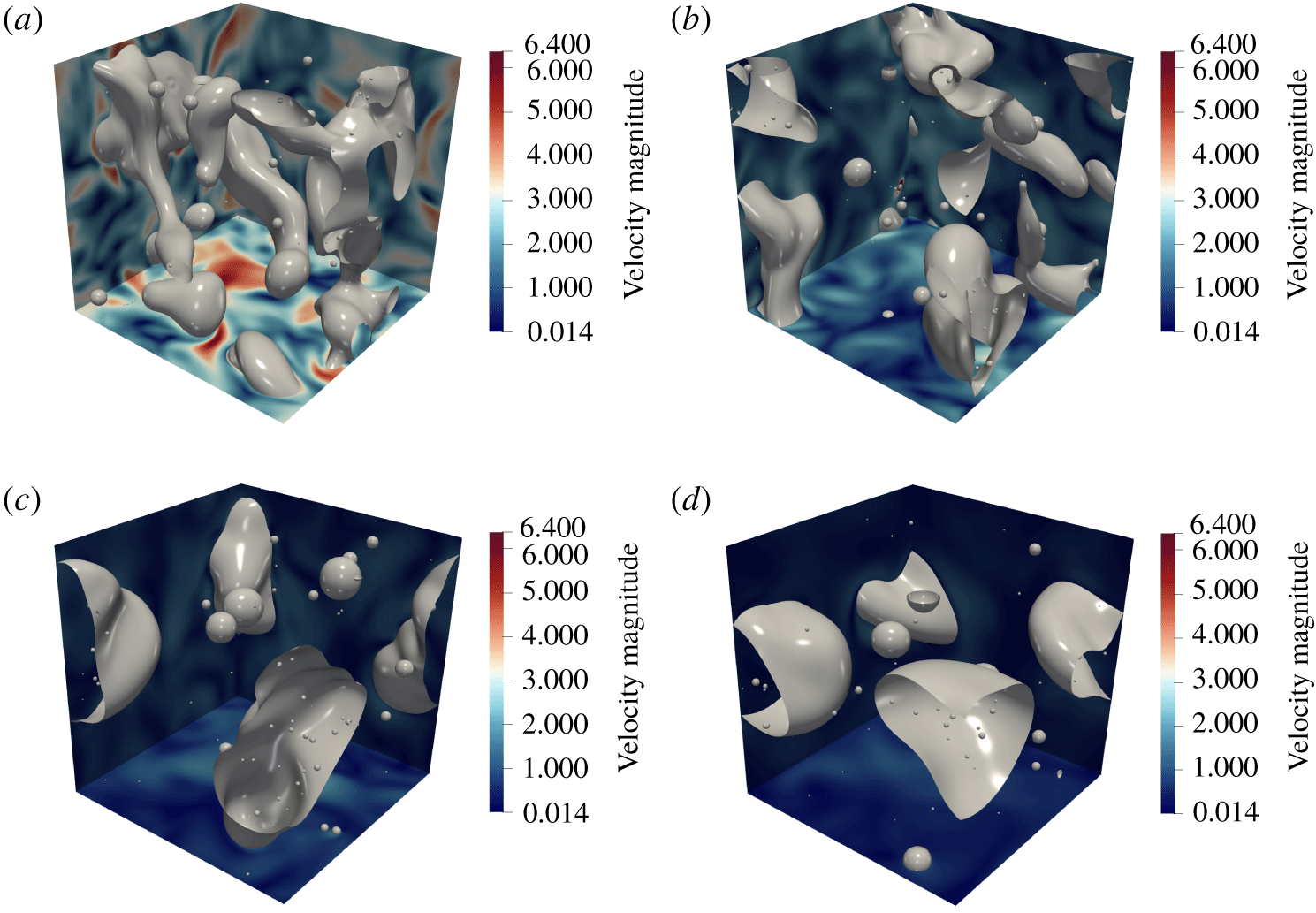
Typical snapshots of decaying liquid–gas turbulence. The liquid–gas interface (the grey surface) corresponds to the zero level-set value. Also portrayed is the velocity magnitude. (a)  $t=0$, (b)
 $t\approx 5{\mathcal{T}}_{i}$, (c)
 $t\approx 10{\mathcal{T}}_{i}$, (d)
 $t\approx 15{\mathcal{T}}_{i}$. From (a) to (d), the turbulent Weber number
 $We_{t}=\unicode[STIX]{x1D70C}_{L}\overline{q^{2}}L_{i}/\unicode[STIX]{x1D6FE}$ is equal to 8.1, 2.4, 1.1 and 0.7.

Typical snapshots of the decaying liquid–gas turbulence simulations are portrayed in figure 2. These are separated by approximately 5 integral time scales  ${\mathcal{T}}_{i}=L_{i}/\sqrt{\overline{q^{2}}}$ (here
 ${\mathcal{T}}_{i}$ is estimated at
 $t=0$ and
 $L_{i}$ is the integral length scale of the velocity field, inferred by integrating the velocity correlation function). At initial time (
 $t=0$), i.e. when forcing is turned off, the liquid structures appear highly tortuous, composed of elongated ligaments, drops and bubbles. Then, the turbulence intensity starts to decrease, as shown by the decrease of fluctuations of the velocity magnitude. Meanwhile, liquid structures progressively coalesce, and surface tension also starts to dominate over inertial forces. Consequently, as turbulence decays, liquid structures grow in size.
3.2 Mesh convergence
Unlike single-phase turbulence simulations, determining a priori the smallest scales to be resolved in DNS of turbulent liquid–gas flows remains as yet unfeasible (Scardovelli & Zaleski Reference Scardovelli and Zaleski1999; Gorokhovski & Saveliev Reference Gorokhovski and Saveliev2003). In interface capturing methods such as the one considered here, break-up of liquid structures occurs automatically when two interface segments are within the same computational grid cell. Therefore, numerical results are inherently grid dependent. As stated by Gorokhovski & Saveliev (Reference Gorokhovski and Saveliev2003), it is however expected that when the resolution is sufficient, the error in liquid volume (∝ the cell volume) becomes negligible compared to the volume of typical liquid structures.
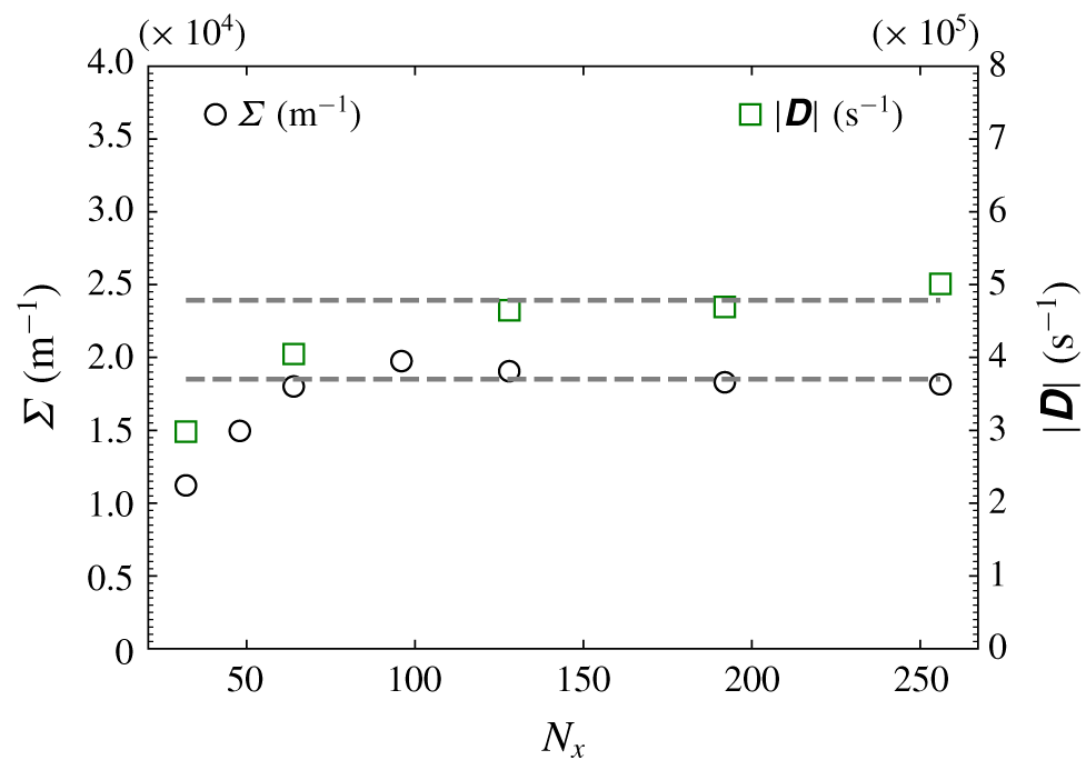
Here, mesh convergence was assessed on the basis of two metrics, one related to the liquid–gas interface, viz. the liquid–gas surface density (the total surface area divided by the simulation volume, noted  $\unicode[STIX]{x1D6F4}$) and one related to the small-scale features of the velocity field, i.e. the norm of the strain rate tensor
 $|\unicode[STIX]{x1D63F}|$. Results are presented in figure 3 where
 $N_{x}=N_{y}=N_{z}$, the number of points in the
 $x$,
 $y$ and
 $z$ directions is varied between 32 and 256. One observes that both metrics nicely converge to a plateau when the resolution increases. Here,
 $|\unicode[STIX]{x1D63F}|$ and
 $\unicode[STIX]{x1D6F4}$ are computed with the forcing active and time averaged over approximately 20 integral time scales;
 $\unicode[STIX]{x1D6F4}$ varies by less than a per cent while
 $|\unicode[STIX]{x1D63F}|$ increases by less than 7 % when
 $N_{x}$ is increased from 192 to 256. A resolution of 2563 is therefore considered as being appropriate. A 5123 simulation might be necessary for confirming this, however, a more stringent test will be discussed later in § 4.3, concluding that a 2563 mesh size is nicely tailored. Hereafter, unless explicitly specified, only the results for this particular mesh size will be discussed. In addition, it is worth stressing that this test of mesh convergence pertains to the case where forcing is active. When forcing is turned off, velocity gradients decrease in magnitude while liquid structures grow in size (see figure 2) meaning that the numerical resolution is enhanced all along the decay.
Mesh convergence of the liquid–gas surface density and velocity strain tensor.

3.3 Anisotropy
The flow is homogeneous in all three directions. Therefore, two-point statistics are spatially averaged. Given the periodic boundary conditions, the  $\boldsymbol{X}$-terms in (2.3) vanish, together with the
 $\boldsymbol{r}$-production term (see appendix B). Consequently, in a triply periodic turbulent two-phase flow, the budget for the total LVF field is the same as the fluctuating field (see appendix C). Further, to improve the statistical relevance of our analysis, we have performed 28 simulations of the decaying flow field starting with different initial conditions, all separated by at least one integral time. In addition to the spatial average, two-point statistics were thus further averaged over these 28 independent realizations. Increments are calculated for separations in the range
 $-N_{x}/2\leqslant (r_{x},r_{y},r_{z})\leqslant N_{x}/2$. Spatially and ensemble averaged statistics are denoted
 $\langle \bullet \rangle _{\mathbb{R},\mathbb{E}}$.
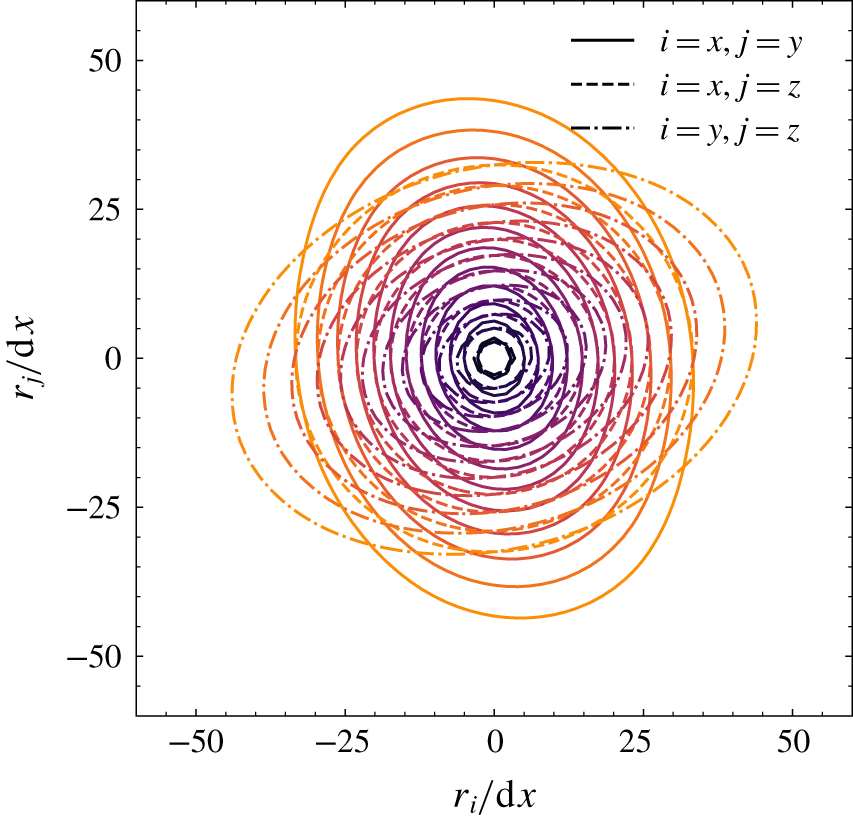
Despite this quite large number of samples, two-point statistics were found to remain substantially anisotropic. Isotropy implies that iso-contours of  $\langle (\unicode[STIX]{x1D6FF}\unicode[STIX]{x1D719})^{2}\rangle _{\mathbb{R},\mathbb{E}}$ in different planes passing by the origin, should form concentric circles. Here, figure 4 emphasizes that second-order statistics of the liquid volume fraction strongly depend on the orientation of the separation vector
 $\boldsymbol{r}$. Although not shown, it also appeared that the degree of anisotropy persists as turbulence decays. To a large extent, this is the result of the lack of statistical convergence of two-point statistics when described in a four-dimensional
 $(\boldsymbol{r},t)$ manifold. Indeed, as seen in figure 2, the number of liquid structures over which statistics are calculated is somewhat limited. For instance, it is observed that the domain contains approximately a dozen liquid structures in figure 2(a), finally coalescing to a few larger drops in figure 2(d). Therefore, even with 28 statistically independent runs, there are not sufficient samples for liquid structures to be isotropically oriented in space and hence for the two-point statistics to lose their dependence on the orientation of the vector
 $\boldsymbol{r}$.
Contours of  $\langle (\unicode[STIX]{x1D6FF}\unicode[STIX]{x1D719})^{2}\rangle _{\mathbb{R},\mathbb{E}}$. Results in different planes are shown, full lines:
 $(r_{x},r_{y},0)$ plane, dashed lines:
 $(r_{x},0,r_{z})$ plane, dash-dotted lines:
 $(0,r_{y},r_{z})$ plane.

3.4 Statistical convergence
Because of this substantial anisotropy, which results from the lack of statistical convergence, we decided to further average two-point statistics over all orientations of the separation vector  $\boldsymbol{r}$. This is achieved by applying a sphere average operation, noted
 $\langle \bullet \rangle _{\mathbb{S}}$, as described in appendix B. Therefore, the two-point budget of the LVF field in decaying turbulence reduces to
 $$\begin{eqnarray}\displaystyle \underbrace{\unicode[STIX]{x2202}_{t}\langle (\unicode[STIX]{x1D6FF}\unicode[STIX]{x1D719})^{2}\rangle _{\mathbb{R},\mathbb{E},\mathbb{S}}}_{Time\,deriv}=-\langle \unicode[STIX]{x1D735}_{\boldsymbol{r}}\boldsymbol{\cdot }\langle (\unicode[STIX]{x1D6FF}\boldsymbol{u})(\unicode[STIX]{x1D6FF}\unicode[STIX]{x1D719})^{2}\rangle _{\mathbb{R},\mathbb{E}}\rangle _{\mathbb{S}}=\underbrace{-\frac{3}{r}\left\langle (\unicode[STIX]{x1D6FF}\boldsymbol{u})\boldsymbol{\cdot }\frac{\boldsymbol{r}}{r}(\unicode[STIX]{x1D6FF}\unicode[STIX]{x1D719})^{2}\right\rangle _{\mathbb{R},\mathbb{E},\unicode[STIX]{x2202}\mathbb{S}}}_{Transfer\,r}, & & \displaystyle\end{eqnarray}$$
with argument list  $(r,t)$, i.e. a two-dimensional problem. In (3.2), the divergence theorem was used to express the spherically averaged divergence of the
 $\boldsymbol{r}$-flux in terms of the normal flux at the sphere boundary
 $\unicode[STIX]{x2202}\mathbb{S}$ (see appendix B). Note that (3.2) is a simplification of (2.3) which applies only to decaying homogeneous flows, the flow under consideration here. For other flow instances, one should refer to the general equation (2.3) and proceed to the relevant simplifications depending on the flow symmetries (invariance with respect to time, invariance by translation in
 $\boldsymbol{X}$-space or invariance by rotation in
 $\boldsymbol{r}$-space). For instance, Thiesset, Dumouchel & Ménard (Reference Thiesset, Dumouchel and Ménard2019a) provide the two-point budget for a time-evolving liquid–gas shear layer.
In order to check the statistical convergence of our results, we plot  $\langle (\unicode[STIX]{x1D6FF}\unicode[STIX]{x1D719})^{2}\rangle _{\mathbb{R},\mathbb{E},\mathbb{S}}$ and
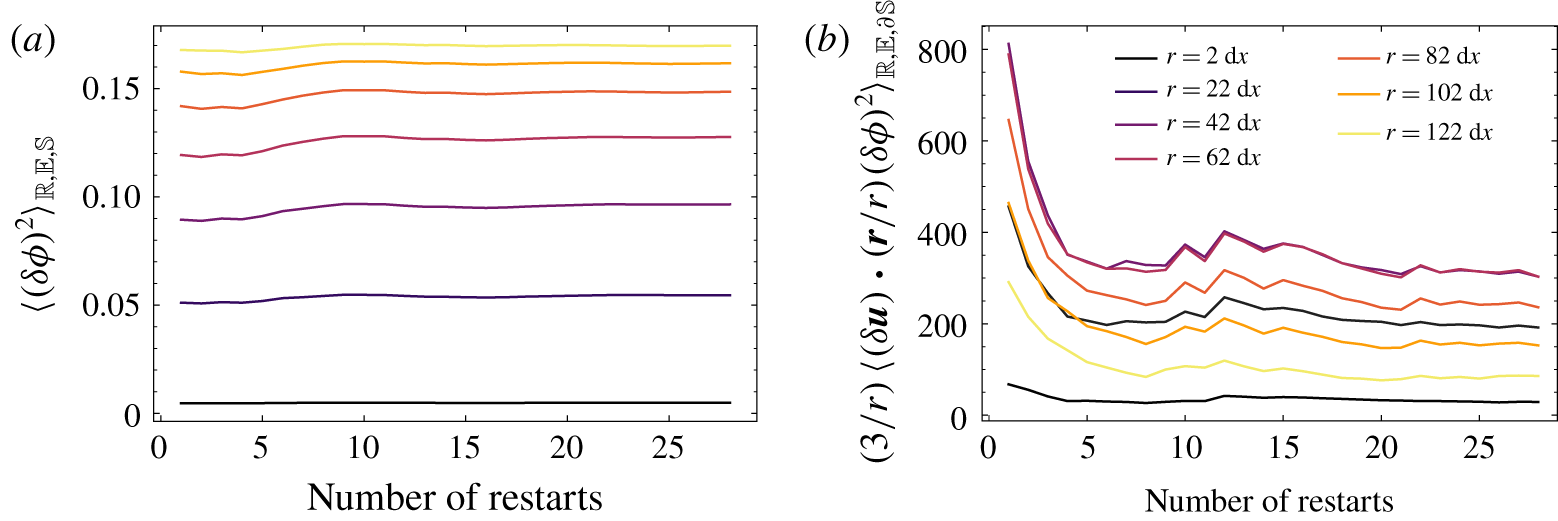
 $(3/r)\langle (\unicode[STIX]{x1D6FF}\boldsymbol{u})\boldsymbol{\cdot }(\boldsymbol{r}/r)(\unicode[STIX]{x1D6FF}\unicode[STIX]{x1D719})^{2}\rangle _{\mathbb{R},\mathbb{E},\unicode[STIX]{x2202}\mathbb{S}}$ as a function of the number of simulation runs for different separations
 $r$ (figure 5). One observes that while second-order statistics (figure 5a) converge rather quickly (≈0.1 % after 28 runs), convergence of third-order statistics (figure 5b) is much slower and it was necessary to run 28 simulations for the transfer term to be within 5 %. This is considered as being sufficient for concluding that the statistics have converged.
Running 28 simulations with the ARCHER code corresponds to approximately 100 000 CPU hours and calculating two-point statistics over approximately 100 snapshots for each of the 28 runs represents approximately 500 000 CPU hours. In total, the database ends up with 10 TB of files. For this reason, it was particularly onerous to address another set of physical parameters (surface tension, total liquid fraction, kinetic energy, etc.) and this aspect is left for future investigations.
Statistical convergence of second- (a) and third-order (b) statistics for different separations,  $r$, as a function of the number of independent simulations used to calculate ensemble averages. Results are for
 $t\approx 7.5{\mathcal{T}}_{i}$.

4 Results
We now aim at evaluating the potential of the two-point statistical analysis of the LVF field using the numerical database described above. This section addresses three main aspects. An analysis of asymptotic scaling of  $\langle (\unicode[STIX]{x1D6FF}\unicode[STIX]{x1D719})^{2}\rangle _{\mathbb{E},\mathbb{R},\mathbb{S}}$ when the separation
 $r$ tends to either large or small values is first performed. This will allow us to emphasize the existence of a characteristic length scale which is closely related to the liquid–gas interface surface density. Next, a similarity analysis is undertaken in order to infer the similarity variables which ought to be used in the scaling of the scale transfer. Finally, light will be shed on the contribution of the different terms of the scale-by-scale budget during the decay of homogeneous liquid–gas turbulence.
4.1 Asymptotic scalings
We start by analysing the asymptotic behaviour of  $\langle (\unicode[STIX]{x1D6FF}\unicode[STIX]{x1D719})^{2}\rangle _{\mathbb{E},\mathbb{R},\mathbb{S}}$ in the limit of small and large separations. To this end, it is worth recalling that the LVF field is rather similar to a so-called asymmetric random telegraphic signal, which features sharp transitions between a value of 1 (corresponding here to the liquid) and 0 (for the gas phase).
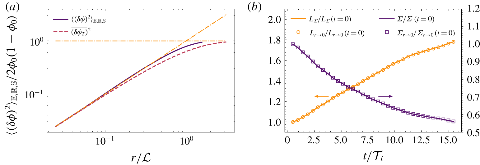
(a) Comparison of  $\langle (\unicode[STIX]{x1D6FF}\unicode[STIX]{x1D719})^{2}\rangle _{\mathbb{E},\mathbb{R},\mathbb{S}}$ at
 $t=4.23{\mathcal{T}}_{i}$ with the second-order structure function of a telegraphic signal with same
 ${\mathcal{L}}$. The asymptotic behaviours at small scales (i.e.
 $r/{\mathcal{L}}$) and large scales (≡1) are also shown as dash-dotted lines. (b) Comparison of
 $\unicode[STIX]{x1D6F4}$ and
 $L_{\unicode[STIX]{x1D6F4}}$ (lines) estimated directly (from the surface area of the zero level set) with those obtained from the limit of
 $\langle (\unicode[STIX]{x1D6FF}\unicode[STIX]{x1D719})^{2}\rangle _{\mathbb{E},\mathbb{R},\mathbb{S}}$ when
 $r\rightarrow 0$ as given by (4.6) and (4.7) (symbols).

Consider a one-dimensional asymmetric random telegraphic signal  $\unicode[STIX]{x1D719}_{T}(x)$ between 0 and 1, where the probability
 $p(\unicode[STIX]{x1D719}_{T}(x)=1)=\unicode[STIX]{x1D719}_{0}$ and
 $p(\unicode[STIX]{x1D719}_{T}(x)=0)=1-\unicode[STIX]{x1D719}_{0}$. In our case,
 $\unicode[STIX]{x1D719}_{0}=0.1$, i.e. the box is filled with 10 % of liquid. The autocorrelation of such a signal, i.e. the average of
 $\unicode[STIX]{x1D719}_{T}(x)\unicode[STIX]{x1D719}_{T}(x+r)$, can be calculated analytically (Machlup Reference Machlup1954; Fitzhugh Reference Fitzhugh1983), and is given by
 $$\begin{eqnarray}\displaystyle R_{\unicode[STIX]{x1D719}_{T}}(r)=\unicode[STIX]{x1D719}_{0}[\unicode[STIX]{x1D719}_{0}+(1-\unicode[STIX]{x1D719}_{0})\text{e}^{-r/{\mathcal{L}}}], & & \displaystyle\end{eqnarray}$$
where  ${\mathcal{L}}$ is a characteristic length scale which relates to the random jump frequency, the probability of transiting from a value of 1 to 0 and vice versa. The mean squared value of
 $\unicode[STIX]{x1D719}_{T}$ is
 $R_{\unicode[STIX]{x1D719}_{T}}(r=0)=\unicode[STIX]{x1D719}_{0}$ and at large separations, the auto-correlation tends to
 $R_{\unicode[STIX]{x1D719}_{T}}(r\rightarrow \infty )=\unicode[STIX]{x1D719}_{0}^{2}$. The fact that the auto-correlation of a telegraphic signal does not tend to 0 when
 $r\rightarrow \infty$ precludes defining an integral length scale. The second-order moment of the increment
 $\unicode[STIX]{x1D6FF}\unicode[STIX]{x1D719}_{T}$, can be expressed in terms of the autocorrelation function, i.e.
 $$\begin{eqnarray}\displaystyle \overline{(\unicode[STIX]{x1D6FF}\unicode[STIX]{x1D719}_{T})^{2}}(r)=2(R_{\unicode[STIX]{x1D719}_{T}}(0)-R_{\unicode[STIX]{x1D719}_{T}}(r))=2(\unicode[STIX]{x1D719}_{0}-R_{\unicode[STIX]{x1D719}_{T}}), & & \displaystyle\end{eqnarray}$$
where again the overbar denotes a suitable average (here a spatial average over the  $x$ axis). Therefore, for a telegraphic signal, we have
 $$\begin{eqnarray}\displaystyle \overline{(\unicode[STIX]{x1D6FF}\unicode[STIX]{x1D719}_{T})^{2}}(r)=2\unicode[STIX]{x1D719}_{0}(1-\unicode[STIX]{x1D719}_{0})[1-\text{e}^{-r/{\mathcal{L}}}]. & & \displaystyle\end{eqnarray}$$
Consequently, at large separations  $\overline{(\unicode[STIX]{x1D6FF}\unicode[STIX]{x1D719}_{T})^{2}}(r)$ tends to a constant equal to
 $2\unicode[STIX]{x1D719}_{0}(1-\unicode[STIX]{x1D719}_{0})$. The limit towards small separations is
 $$\begin{eqnarray}\displaystyle \lim _{r\rightarrow 0}\overline{(\unicode[STIX]{x1D6FF}\unicode[STIX]{x1D719}_{T})^{2}}(r)=2\unicode[STIX]{x1D719}_{0}(1-\unicode[STIX]{x1D719}_{0})\frac{r}{{\mathcal{L}}}+O\left(\frac{r^{2}}{{\mathcal{L}}^{2}}\right). & & \displaystyle\end{eqnarray}$$
Equation (4.4) indicates that the second-order structure function of a telegraphic signal  $\unicode[STIX]{x1D719}_{T}$ is proportional to
 $r$ when
 $r$ is small compared to
 ${\mathcal{L}}$. Equation (4.4) allows calculation of the characteristic length scale
 ${\mathcal{L}}$ as
 $$\begin{eqnarray}\displaystyle {\mathcal{L}}=2\unicode[STIX]{x1D719}_{0}(1-\unicode[STIX]{x1D719}_{0})\left[\lim _{r\rightarrow 0}\frac{\overline{(\unicode[STIX]{x1D6FF}\unicode[STIX]{x1D719}_{T})^{2}}(r)}{r}\right]^{-1}. & & \displaystyle\end{eqnarray}$$
The comparison between  $\langle (\unicode[STIX]{x1D6FF}\unicode[STIX]{x1D719})^{2}\rangle _{\mathbb{E},\mathbb{R},\mathbb{S}}$ estimated from the DNS and
 $\overline{(\unicode[STIX]{x1D6FF}\unicode[STIX]{x1D719}_{T})^{2}}$ is portrayed in figure 6(a). Results are shown for an arbitrary time
 $t=4.23{\mathcal{T}}_{i}$ but similar behaviours were observed for all
 $t$. In figure 6,
 $\langle (\unicode[STIX]{x1D6FF}\unicode[STIX]{x1D719})^{2}\rangle _{\mathbb{E},\mathbb{R},\mathbb{S}}$ and
 $\overline{(\unicode[STIX]{x1D6FF}\unicode[STIX]{x1D719}_{T})^{2}}$ are normalized by
 $2\unicode[STIX]{x1D719}_{0}(1-\unicode[STIX]{x1D719}_{0})$. At large scales, we then observe that both curves tend to an asymptotic value of 1 consistently with the aforementioned considerations. As a consequence, the limit at large
 $r$ can be used to compute the total volume occupied by the liquid
 $\unicode[STIX]{x1D719}_{0}$. At small separations (
 $r/{\mathcal{L}}\leqslant 0.1$),
 $\langle (\unicode[STIX]{x1D6FF}\unicode[STIX]{x1D719})^{2}\rangle _{\mathbb{E},\mathbb{R},\mathbb{S}}$ approaches
 $\overline{(\unicode[STIX]{x1D6FF}\unicode[STIX]{x1D719}_{T})^{2}}$ and appears to be nicely proportional to
 $r/{\mathcal{L}}$. Therefore, the asymptotic scaling at large and small scales is in perfect agreement with an asymmetric telegraphic signal. It is further worth noting that, at small scales, the scaling
 $\langle (\unicode[STIX]{x1D6FF}\unicode[STIX]{x1D719})^{2}\rangle _{\mathbb{E},\mathbb{R},\mathbb{S}}\propto r/{\mathcal{L}}$ extends up to scales
 $r\approx {\mathcal{L}}/2$. The fact that at small scales,
 $\langle (\unicode[STIX]{x1D6FF}\unicode[STIX]{x1D719})^{2}\rangle _{\mathbb{E},\mathbb{R},\mathbb{S}}\propto r/{\mathcal{L}}$ precludes defining a Taylor microscale for the LVF field since the latter assumes a
 $r^{2}$ scaling of second-order structure functions at small scales. Therefore, by analogy with the asymmetric random telegraphic signal, it appears that neither an integral length nor a Taylor length scale can be defined and that the only length scale which one can define is
 ${\mathcal{L}}$ as given by (4.5).
As mentioned earlier,  ${\mathcal{L}}$ relates to the random jump frequency. Hence, there should exist a link between
 ${\mathcal{L}}$ and a length scale based on the liquid–gas surface area. Anez et al. (Reference Anez, Ahmed, Hecht, Duret, Reveillon and Demoulin2019) proposed a slight modification of the interface length scale first introduced by Lebas et al. (Reference Lebas, Menard, Beau, Berlemont and Demoulin2009) which is written
 $$\begin{eqnarray}\displaystyle L_{\unicode[STIX]{x1D6F4}}=\frac{6\unicode[STIX]{x1D719}_{0}(1-\unicode[STIX]{x1D719}_{0})}{\unicode[STIX]{x1D6F4}}, & & \displaystyle\end{eqnarray}$$
where  $\unicode[STIX]{x1D6F4}$ is the surface density (the surface area divided by total volume) of the liquid–gas interface. Here,
 $L_{\unicode[STIX]{x1D6F4}}$ can be interpreted as a generalization of Sauter mean diameter of non-spherical objects, hence the pre-factor 6. A rather similar definition for
 $L_{\unicode[STIX]{x1D6F4}}$ was given by Peters (Reference Peters1992, see equation (5.2)) to describe turbulent premixed flames using a level-set formulation. By analysing the DNS data, we found out that
 $$\begin{eqnarray}\displaystyle \unicode[STIX]{x1D6F4}=3\lim _{r\rightarrow 0}\frac{\langle (\unicode[STIX]{x1D6FF}\unicode[STIX]{x1D719})^{2}\rangle _{\mathbb{ E},\mathbb{R}}}{r}. & & \displaystyle\end{eqnarray}$$
Equation (4.7) can most likely be proven analytically knowing that  $\unicode[STIX]{x1D6F4}=\langle |\unicode[STIX]{x1D735}\unicode[STIX]{x1D719}|\rangle _{\mathbb{R}}$. However, we were not able to end up with a rigorous demonstration for general cases. In the scientific community of porous media or composite materials, the phase indicator function is often used as a scalar representing the different phases composing the material. It thus has some degrees of resemblance to the LVF field. For instance, equation (4.1) is often used to characterize the structure of a particular type of porous medium, known as the Debye random medium (Debye & Bueche Reference Debye and Bueche1949; Debye, Anderson & Brumberger Reference Debye, Anderson and Brumberger1957). By scrutinizing this literature, we discovered that Yeong & Torquato (Reference Yeong and Torquato1998) derived the same expression as (4.7) (see their equation (8)), but again their methodology does not address very general cases. Debye et al. (Reference Debye, Anderson and Brumberger1957) proposed a similar relation as (4.7), except that they found a prefactor of 8/3 instead of 3. At this stage, we thus have no other solutions than numerically validating (4.7).
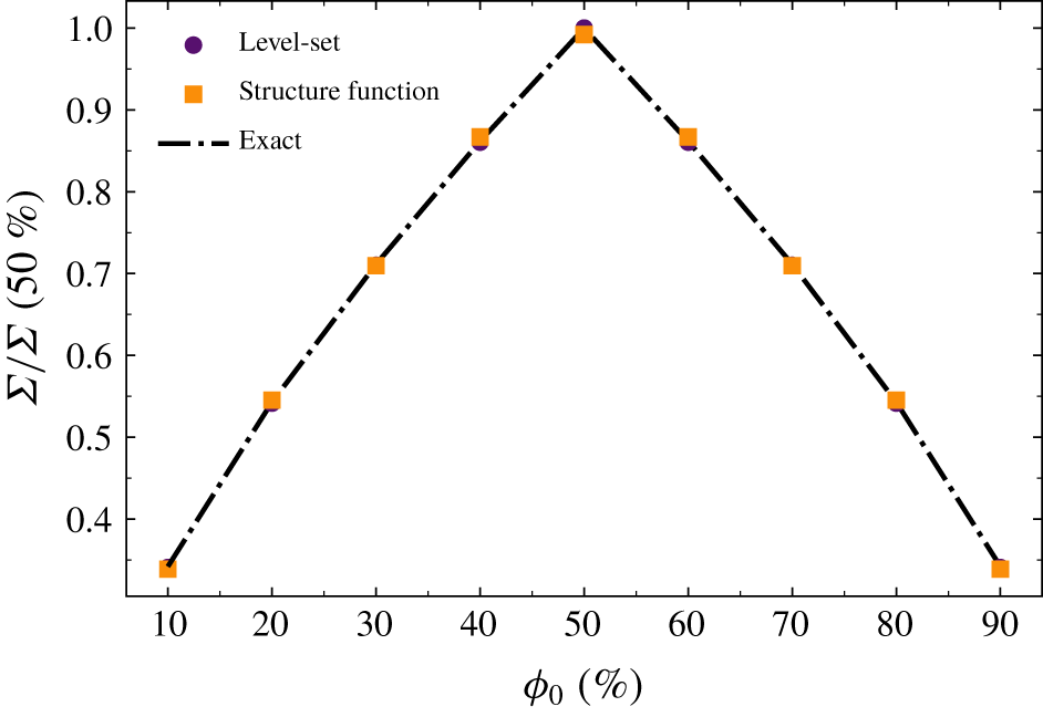
Comparison of  $\unicode[STIX]{x1D6F4}$ as estimated directly by computing the surface area of the zero level set and the values obtained from (4.7) is shown in figure 6(b). The two curves are almost undistinguishable from each other, indicating that, although not demonstrated mathematically, equation (4.7) is correct. We have also tested that (4.7) remains valid when
 $\unicode[STIX]{x1D719}_{0}$ is varied (see appendix D). Consequently, the values for
 $L_{\unicode[STIX]{x1D6F4}}$ estimated either from the surface density or from the limit of
 $\langle (\unicode[STIX]{x1D6FF}\unicode[STIX]{x1D719})^{2}\rangle _{\mathbb{E},\mathbb{R}}$ at small scales are also in perfect agreement (see figure 6b). Equation (4.7) yields
 ${\mathcal{L}}\equiv L_{\unicode[STIX]{x1D6F4}}$. In other words, the only relevant length scale that emerges for the LVF field is
 $L_{\unicode[STIX]{x1D6F4}}$ as defined by either (4.5) or (4.6).
To summarize, the asymmetric telegraphic signal is a nice surrogate of the LVF field for analysing the asymptotic scaling of  $\langle (\unicode[STIX]{x1D6FF}\unicode[STIX]{x1D719})^{2}\rangle _{\mathbb{E},\mathbb{R}}$ at either large or small scales. We have proven that
 $\langle (\unicode[STIX]{x1D6FF}\unicode[STIX]{x1D719})^{2}\rangle _{\mathbb{E},\mathbb{R}}$ contains information about the geometrical nature of the liquid–gas interface (its surface area) and the total liquid fraction
 $\unicode[STIX]{x1D719}_{0}$. Nevertheless, the distribution
 $\overline{(\unicode[STIX]{x1D6FF}\unicode[STIX]{x1D719}_{T})^{2}}$ departs significantly from
 $\langle (\unicode[STIX]{x1D6FF}\unicode[STIX]{x1D719})^{2}\rangle _{\mathbb{E},\mathbb{R}}$ at intermediate scales, which indicates that the LVF field is not a purely random field but has certain features representative of the morphology of the liquid structures. Comparing
 $\langle (\unicode[STIX]{x1D6FF}\unicode[STIX]{x1D719})^{2}\rangle _{\mathbb{E},\mathbb{R}}$ and
 $\overline{(\unicode[STIX]{x1D6FF}\unicode[STIX]{x1D719}_{T})^{2}}$ could possibly be exploited in future investigations to shed light on the peculiar geometrical facets of the liquid–gas interface.
4.2 Similarity analysis
Finding which similarity variables are the most appropriate for normalizing two-point statistics provides insights into the prominent mechanisms at play in a given region of flow and over a given range of scales. Potentially, self-similarity can further reduce scale-by-scale budgets (i.e. partial differential equations) to ordinary differential equations, thereby leading to predictions of one-point statistics and simple closures of the scale-by-scale budget.
In the light of the methodology developed for single-phase turbulence, we apply a similarity analysis to the budget equation (3.2). To this end, we start by writing second and crossed moments of LVF increments in the form
 $$\begin{eqnarray}\displaystyle & \displaystyle \langle (\unicode[STIX]{x1D6FF}\unicode[STIX]{x1D719})^{2}\rangle _{\mathbb{R},\mathbb{E},\mathbb{S}}=e(\unicode[STIX]{x1D709})E^{\ast }(t), & \displaystyle\end{eqnarray}$$
 $$\begin{eqnarray}\displaystyle & \displaystyle \frac{3}{r}\left\langle (\unicode[STIX]{x1D6FF}\boldsymbol{u})\boldsymbol{\cdot }\frac{\boldsymbol{r}}{r}(\unicode[STIX]{x1D6FF}\unicode[STIX]{x1D719})^{2}\right\rangle _{\mathbb{R},\mathbb{E},\unicode[STIX]{x2202}\mathbb{S}}=g(\unicode[STIX]{x1D709})G^{\ast }(t), & \displaystyle\end{eqnarray}$$
 $\unicode[STIX]{x1D709}=r/\unicode[STIX]{x1D706}(t)$ where
 $\unicode[STIX]{x1D706}(t)$ is the similarity length scale which depends on time but is a priori unknown. Here,
 $E^{\ast }(t)$ and
 $G^{\ast }(t)$ are two normalizing quantities which pertain to second and crossed moments, respectively. As was done by e.g. George (Reference George1992a), Antonia et al. (Reference Antonia, Smalley, Zhou, Anselmet and Danaila2003) and Burattini et al. (Reference Burattini, Antonia and Danaila2005b), second-order structure functions are generally normalized by their value when the separation tends to large values. Here, we proceed similarly and assume
 $$\begin{eqnarray}\displaystyle E^{\ast }(t)=\lim _{r\rightarrow \infty }\langle (\unicode[STIX]{x1D6FF}\unicode[STIX]{x1D719})^{2}\rangle _{\mathbb{R},\mathbb{E},\mathbb{S}}=2\unicode[STIX]{x1D719}_{0}(1-\unicode[STIX]{x1D719}_{0}). & & \displaystyle\end{eqnarray}$$
It is therefore assumed that  $E^{\ast }=\text{const}$. Injecting (4.8) into (3.2), yields
 $$\begin{eqnarray}\displaystyle \unicode[STIX]{x2202}_{t}e(\unicode[STIX]{x1D709})E^{\ast }(t)=-g(\unicode[STIX]{x1D709})G^{\ast }(t). & & \displaystyle\end{eqnarray}$$
Assuming  $E^{\ast }=\text{const.}$, we have
 $$\begin{eqnarray}\displaystyle E^{\ast }(t)\{\unicode[STIX]{x2202}_{\unicode[STIX]{x1D709}}e(\unicode[STIX]{x1D709})\}\{\unicode[STIX]{x2202}_{t}\unicode[STIX]{x1D709}(t)\}=-g(\unicode[STIX]{x1D709})G^{\ast }(t) & & \displaystyle\end{eqnarray}$$
recalling that  $\unicode[STIX]{x2202}_{t}\unicode[STIX]{x1D709}(t)=\unicode[STIX]{x1D709}\unicode[STIX]{x2202}_{t}\log \unicode[STIX]{x1D706}$, we end up with
 $$\begin{eqnarray}\displaystyle [E^{\ast }\unicode[STIX]{x2202}_{t}\log \unicode[STIX]{x1D706}]\unicode[STIX]{x1D709}\unicode[STIX]{x2202}_{\unicode[STIX]{x1D709}}e(\unicode[STIX]{x1D709})=g(\unicode[STIX]{x1D709})[G^{\ast }(t)]. & & \displaystyle\end{eqnarray}$$
Self-similarity implies that the terms which depend only on time (the terms within brackets) should behave similarly with respect to time, viz.
 $$\begin{eqnarray}\displaystyle G^{\ast }(t)\propto \unicode[STIX]{x2202}_{t}\log \unicode[STIX]{x1D706}(t). & & \displaystyle\end{eqnarray}$$
However, it is not revealed which length scale  $\unicode[STIX]{x1D706}(t)$ should be used for normalizing the separation
 $r$. Given the asymptotic scaling described in the previous section, it worth testing
 $L_{\unicode[STIX]{x1D6F4}}$ as the similarity length scale. Then, it is expected that
 $$\begin{eqnarray}\displaystyle G^{\ast }(t)\propto -\unicode[STIX]{x2202}_{t}\log \unicode[STIX]{x1D6F4}=\mathbb{K}_{\unicode[STIX]{x1D6F4}}. & & \displaystyle\end{eqnarray}$$
If  $L_{\unicode[STIX]{x1D6F4}}$ were to be used as a similarity length scale, then the transfer term should scale with the stretch rate
 $\mathbb{K}_{\unicode[STIX]{x1D6F4}}$ of the liquid–gas interface.
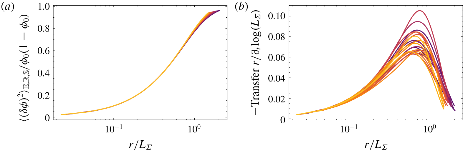
Assessment of the degree of self-similarity of (a) second and (b) crossed moments when the separation  $r$ is normalized by
 $L_{\unicode[STIX]{x1D6F4}}$. The different colours from dark to light correspond to increasing time during the decay.

The adequacy of the proposed similarity variables to normalize the scale distribution and scale transfer of the LVF is presented in figures 7(a) and 7(b), respectively. The scale distributions  $\langle (\unicode[STIX]{x1D6FF}\unicode[STIX]{x1D719})^{2}\rangle _{\mathbb{R},\mathbb{E},\mathbb{S}}$ collapse very nicely when the separation
 $r$ is normalized by
 $L_{\unicode[STIX]{x1D6F4}}$. However, self-similarity is not complete, i.e. it does not span the entire range of scales, but appears to be accurately satisfied up to
 $r\approx L_{\unicode[STIX]{x1D6F4}}/2$. This means that
 $L_{\unicode[STIX]{x1D6F4}}$ (and thus
 $\unicode[STIX]{x1D6F4}$) is the relevant quantity for characterizing the time evolution of
 $\langle (\unicode[STIX]{x1D6FF}\unicode[STIX]{x1D719})^{2}\rangle _{\mathbb{R},\mathbb{E},\mathbb{S}}$, at least at small scales. As far as the transfer term in (3.2) is concerned, i.e.
 $\text{Transfer}\,r=-3/r\langle (\unicode[STIX]{x1D6FF}\boldsymbol{u})\boldsymbol{\cdot }\boldsymbol{r}/r(\unicode[STIX]{x1D6FF}\unicode[STIX]{x1D719})^{2}\rangle _{\mathbb{R},\mathbb{E},\unicode[STIX]{x2202}\mathbb{S}}$ (figure 7b), although the scatter is significant especially at large scales (
 $r\gtrsim L_{\unicode[STIX]{x1D6F4}}/2$), it appears that again
 $L_{\unicode[STIX]{x1D6F4}}$ and thus
 $\mathbb{K}_{\unicode[STIX]{x1D6F4}}$ is a relevant similarity variable. In other words, time variations of
 $\langle (\unicode[STIX]{x1D6FF}\unicode[STIX]{x1D719})^{2}\rangle _{\mathbb{R},\mathbb{E},\mathbb{S}}$ for all scales
 $r\lesssim L_{\unicode[STIX]{x1D6F4}}/2$ are uniquely determined by the stretch rate. Consequently, in analogy with the Kolmogorov or Batchelor scaling of second-order structure functions for either the velocity or scalar field, the stretch rate plays here the same role as the kinetic energy or scalar dissipation rate. This statement can be further illustrated by taking the limit at small separations of the scale-by-scale budget. Plugging (4.7) into (3.2) yields
 $$\begin{eqnarray}\displaystyle -\frac{3}{r}\left\langle (\unicode[STIX]{x1D6FF}\boldsymbol{u})\boldsymbol{\cdot }\frac{\boldsymbol{r}}{r}(\unicode[STIX]{x1D6FF}\unicode[STIX]{x1D719})^{2}\right\rangle _{\mathbb{R},\mathbb{E},\unicode[STIX]{x2202}\mathbb{S}}=2\unicode[STIX]{x1D719}_{0}(1-\unicode[STIX]{x1D719}_{0})\frac{\mathbb{K}_{\unicode[STIX]{x1D6F4}}r}{L_{\unicode[STIX]{x1D6F4}}}, & & \displaystyle\end{eqnarray}$$
for all  $r\ll L_{\unicode[STIX]{x1D6F4}}$. Equation (4.15) can be viewed as the equivalent for a non-diffusive scalar such as the LVF, of the Kolmogorov (Reference Kolmogorov1941a) four-fifths law or the Yaglom (Reference Yaglom1949) four-thirds law. It suggests that, for scales sufficiently small compared to
 $L_{\unicode[STIX]{x1D6F4}}$, the transfer term scales with
 $r/L_{\unicode[STIX]{x1D6F4}}$ and is proportional to the stretch rate. This leads us to the startling conclusion that the equivalent for a non-diffusive scalar of the scalar dissipation rate is the stretch rate of the interface separating
 $\unicode[STIX]{x1D719}=0$ and
 $\unicode[STIX]{x1D719}=1$.
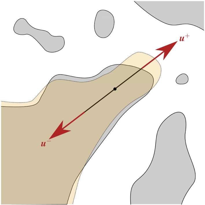
Schematic representation of  $(\unicode[STIX]{x1D6FF}\boldsymbol{u})(\unicode[STIX]{x1D6FF}\unicode[STIX]{x1D719})^{2}$.

The relevance of the stretch rate as a similarity variable for the energy transfer can be illustrated as in figure 8. Consider the case where an interface is present between the two points  $\boldsymbol{x}^{+}$ and
 $\boldsymbol{x}^{-}$, meaning that
 $\unicode[STIX]{x1D6FF}\unicode[STIX]{x1D719}\neq 0$. Two such cases are represented in figure 8 and are labelled (1) and (2). Here,
 $(\unicode[STIX]{x1D6FF}\boldsymbol{u})\boldsymbol{\cdot }\boldsymbol{r}(\unicode[STIX]{x1D6FF}\unicode[STIX]{x1D719})^{2}$ is non-zero if
 $(\unicode[STIX]{x1D6FF}\boldsymbol{u})\boldsymbol{\cdot }\boldsymbol{r}$ is non-zero, i.e. there exists a velocity gradient along the direction
 $\boldsymbol{r}$. When
 $(\unicode[STIX]{x1D6FF}\boldsymbol{u})\boldsymbol{\cdot }\boldsymbol{r}>0$ (Case 1), the liquid structure undergoes a stretching mechanism along the direction
 $\boldsymbol{r}$ leading to an increase in size in this particular direction (this is illustrated by the green patch in figure 8). On contrary, when
 $(\unicode[STIX]{x1D6FF}\boldsymbol{u})\boldsymbol{\cdot }\boldsymbol{r}<0$ (Case 2), the liquid structure is submitted to a compression effect and its size tends to decrease (as illustrated by the green patch in figure 8). Therefore, this simple sketch illustrates that the mechanism behind the scale energy transfer is closely related to the stretch/compression rate acting at some scale
 $r$. The same reasoning was often stated for the turbulent cascade as being caused by vortex stretching (see Lundgren (Reference Lundgren1982), for instance).
We note that the turbulence characteristics (i.e. the kinetic energy, the integral and Taylor length scales) do not appear as plausible similarity variables in the scale transport of the LVF field. This proves again that the effect of turbulence is implicit in this theoretical framework. Turbulence shows itself implicitly through its effect on the liquid–gas interface and more specifically on the surface density and stretch rate.
4.3 LVF budget and flux decomposition
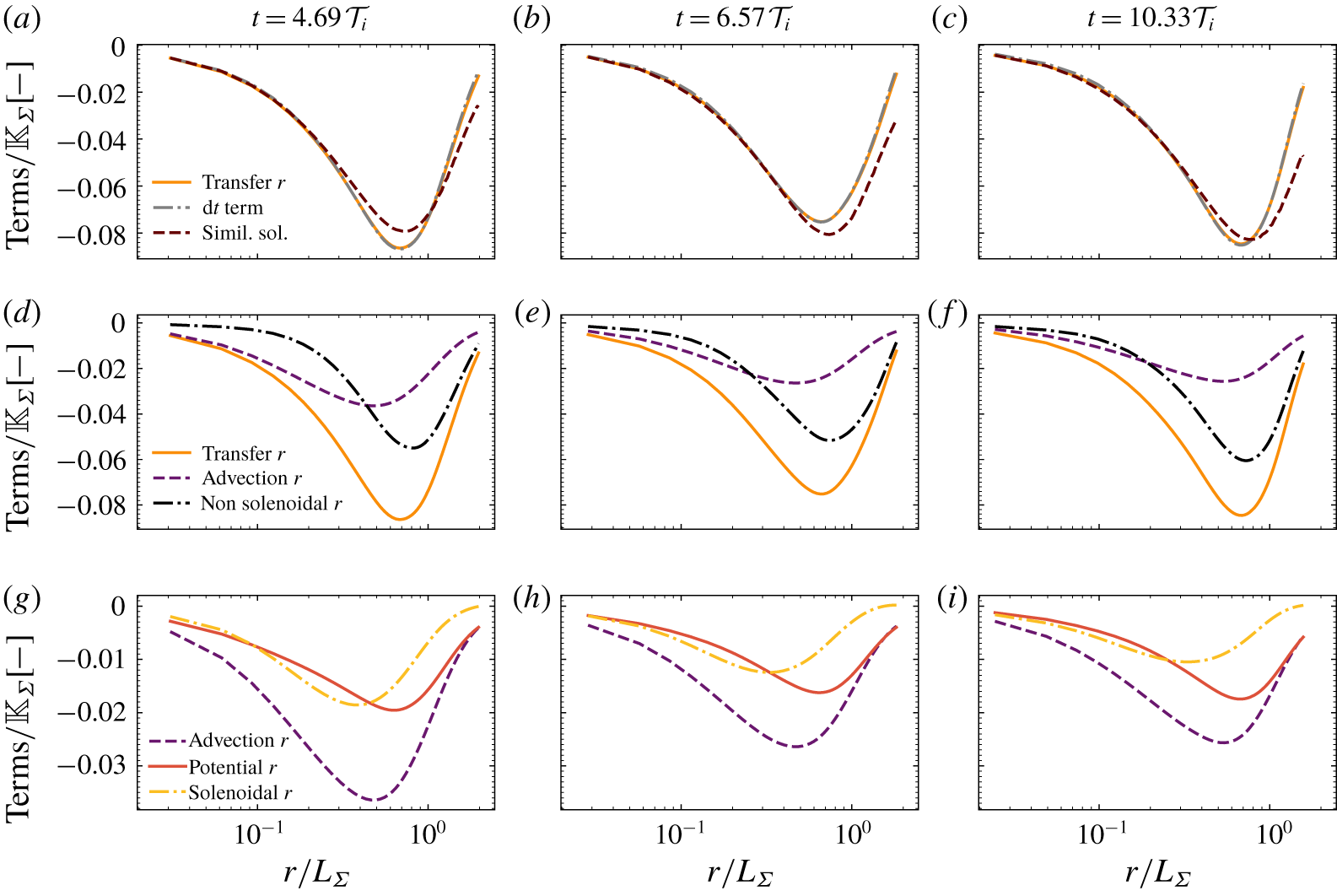
We now turn our attention to the contribution of each term of the scale-by-scale budget equation (3.2). We start by verifying that the budget given by (3.2) is accurately closed. Results are presented in figure 9(a–c) for three arbitrary time values during the decay. There were not noticeable differences for other time values. It appears that the time derivative term is perfectly balanced by the transfer term. Because (3.2) is exact, this represents a very stringent test of the accuracy of the simulation results. In addition to the mesh convergence presented in § 3.2, it thus reinforces that the spatial resolution used for the present simulations is adequate. Figure 9(a–c) also presents the profiles of the transfer term as calculated from the similarity solution  $g(\unicode[STIX]{x1D709})=-\unicode[STIX]{x1D709}\unicode[STIX]{x2202}_{\unicode[STIX]{x1D709}}e(\unicode[STIX]{x1D709})$. The latter appears to be well suited for describing the scale transfer at small scales (
 $r\lesssim L_{\unicode[STIX]{x1D6F4}}/2$), i.e. over the range of scales where similarity applies.
It is worth noting that in our case, the  $r$-transfer term in (3.2), i.e.
 $\propto -\langle (\unicode[STIX]{x1D6FF}\boldsymbol{u})\boldsymbol{\cdot }\boldsymbol{r}(\unicode[STIX]{x1D6FF}\unicode[STIX]{x1D719})^{2}\rangle _{\mathbb{R},\mathbb{E},\unicode[STIX]{x2202}\mathbb{S}}$ is negative irrespective of
 $r$. This indicates that, on average, liquid structures are growing in size. This is consistent with figure 2, where it was observed that initially stretched structures (mostly ligaments, see figure 2a) relax to more ‘spherical’ objects (figure 2d) due to coalescence and surface tension effects. Therefore, for the LVF to be conserved, liquid structures which are longitudinally decreasing in size, concomitantly expand in the ligament transverse directions. Averaging over all directions
 $\boldsymbol{r}$ leads to an increase in size, viz. on average the transfer of LVF is directed towards large scales. This is a very peculiar difference from a diffusive passive scalar, for which the transfer term has the opposite sign (i.e. is directed towards small scales) and diffusion is the driving mechanism leading, on average, to an increase in size of the turbulent scales (Danaila et al. Reference Danaila, Anselmet, Zhou and Antonia1999; Antonia & Orlandi Reference Antonia and Orlandi2004; Gauding et al. Reference Gauding, Wick, Pitsch and Peters2014, for instance). In case of turbulent liquid–gas flows, the LVF does not diffuse, and thus surface tension and coalescence are the only mechanisms responsible for the relaxation of elongated ligaments into larger (on average) liquid structures.
(a–c) Contribution of the different terms of the budget equation (3.2). The similarity solution  $g(\unicode[STIX]{x1D709})=-\unicode[STIX]{x1D709}\unicode[STIX]{x2202}_{\unicode[STIX]{x1D709}}e(\unicode[STIX]{x1D709})$ is also displayed as dotted lines. (d–f) Decomposition of the
 $r$-transfer term into a local and a non-local transfer term (4.16). (g–i) Decomposition of the
 $r$-advection term using a potential and solenoidal velocity (4.17). Results are presented for
 $t=4.69,6.57,10.33{\mathcal{T}}_{i}$.

We now turn our attention to the decomposition of the transfer term into local and non-local interactions. Spherically averaging (2.7) enables writing the transfer term in the form
 $$\begin{eqnarray}\displaystyle \underbrace{-\left\langle (\unicode[STIX]{x1D6FF}\boldsymbol{u})\boldsymbol{\cdot }\frac{\boldsymbol{r}}{r}(\unicode[STIX]{x1D6FF}\unicode[STIX]{x1D719})^{2}\right\rangle _{\mathbb{E},\mathbb{R},\unicode[STIX]{x2202}\mathbb{S}}}_{Transfer\,r}=\underbrace{-\langle \boldsymbol{w}_{\boldsymbol{r}}\boldsymbol{\cdot }\unicode[STIX]{x1D735}\langle (\unicode[STIX]{x1D6FF}\unicode[STIX]{x1D719})^{2}\rangle _{\mathbb{ E},\mathbb{R}}\rangle _{\mathbb{S}}}_{Advection\,r}-\underbrace{\langle \langle (\unicode[STIX]{x1D6FF}\unicode[STIX]{x1D719})^{2}\rangle _{\mathbb{ E},\mathbb{R}}\unicode[STIX]{x1D735}\boldsymbol{\cdot }\boldsymbol{w}_{\boldsymbol{r}}\rangle _{\mathbb{S}}}_{Non\,Solenoidal\,r}, & & \displaystyle\end{eqnarray}$$
where  $\boldsymbol{w}_{\boldsymbol{r}}$ is given by (2.6a). As demonstrated in § 2.3, the decomposition equation (4.16) is a way of decomposing the transfer term into a local purely convective term and a source term associated with non-local interactions in scale space. The contribution of these two mechanisms with respect to the separation
 $r$ is presented in figure 9(d–f) for the same three time values. Globally, the amplitudes of the local and non-local processes have the same order of magnitude. The non-local process peaks at larger scales than the advection mechanism. At small scales (
 $r\lesssim 0.3L_{\unicode[STIX]{x1D6F4}}$), the advection dominates slightly over the non-local process. The contrary is observed at rather large scales
 $r\gtrsim 0.3L_{\unicode[STIX]{x1D6F4}}$.
The two-point analysis indicates a noticeable contribution of non-local interactions in scale space, i.e. two separated scales can interact although they are very different in size. We explain this observation by the effect of surface tension. To illustrate this statement, consider the case of the Plateau–Rayleigh instability of a liquid ligament. Surface tension forces depend on the local mean curvature. Along the ligament axis, pressure is thus high at the crests (where curvature is negative) and low at the troughs (positive curvature). This effect is known as the capillary bridge. Surface tension forces will then tend to amplify the contraction (expansion) effect at the neck (crests), ultimately leading to pinch-off, break-up, followed by the retraction of the neck and the formation of one or several droplets. Before break-up, the size of neck and that of the forming droplet can be very different. However, they strongly interact through the capillary bridge, this interaction being mediated by the pressure field, an essentially non-local process. Therefore, this simple example suggests that, because of surface tension effects, non-local interactions can play an essential role in the scale transport of the LVF.
We further apply a Helmholtz decomposition to the convection velocity  $\boldsymbol{w}_{\boldsymbol{r}}$, thereby allowing us to rewrite the
 $r$-advection term in the form
 $$\begin{eqnarray}\displaystyle \underbrace{-\langle \boldsymbol{w}_{\boldsymbol{r}}\boldsymbol{\cdot }\unicode[STIX]{x1D735}\langle (\unicode[STIX]{x1D6FF}\unicode[STIX]{x1D719})^{2}\rangle _{\mathbb{E},\mathbb{R}}\rangle _{\mathbb{S}}}_{Advection\,r}=\underbrace{-\langle \boldsymbol{w}_{\boldsymbol{r}}^{\boldsymbol{p}\boldsymbol{o}\boldsymbol{t}}\boldsymbol{\cdot }\unicode[STIX]{x1D735}\langle (\unicode[STIX]{x1D6FF}\unicode[STIX]{x1D719})^{2}\rangle _{\mathbb{E},\mathbb{R}}\rangle _{\mathbb{S}}}_{Potential\,r}\underbrace{-\langle \boldsymbol{w}_{\boldsymbol{r}}^{\boldsymbol{s}\boldsymbol{o}\boldsymbol{l}}\boldsymbol{\cdot }\unicode[STIX]{x1D735}\langle (\unicode[STIX]{x1D6FF}\unicode[STIX]{x1D719})^{2}\rangle _{\mathbb{E},\mathbb{R}}\rangle _{\mathbb{S}}}_{Solenoidal\,r}, & & \displaystyle\end{eqnarray}$$
where  $\boldsymbol{w}_{\boldsymbol{r}}^{\boldsymbol{p}\boldsymbol{o}\boldsymbol{t}}$ and
 $\boldsymbol{w}_{\boldsymbol{r}}^{\boldsymbol{s}\boldsymbol{o}\boldsymbol{l}}$ are the potential (curl-free) and solenoidal (divergence-free) components, respectively. For doing this, we solve the Poisson equation
 $$\begin{eqnarray}\displaystyle \unicode[STIX]{x1D735}_{\boldsymbol{r}}\boldsymbol{\cdot }\boldsymbol{w}_{\boldsymbol{r}}=-\unicode[STIX]{x1D735}_{\boldsymbol{r}}\boldsymbol{\cdot }(\unicode[STIX]{x1D735}_{\boldsymbol{r}}P_{r}) & & \displaystyle\end{eqnarray}$$
and compute  $\boldsymbol{w}_{\boldsymbol{r}}^{\boldsymbol{p}\boldsymbol{o}\boldsymbol{t}}=-\unicode[STIX]{x1D735}_{\boldsymbol{r}}P_{r}$ and
 $\boldsymbol{w}_{\boldsymbol{r}}^{\boldsymbol{s}\boldsymbol{o}\boldsymbol{l}}=\boldsymbol{w}_{\boldsymbol{r}}-\boldsymbol{w}_{\boldsymbol{r}}^{\boldsymbol{p}\boldsymbol{o}\boldsymbol{t}}$. Equation (4.18) is solved using the MINRES algorithm implemented in the Scipy Library of Python. Given the symmetry of the problem, zero normal gradient boundary conditions were used. Results are presented in figure 9(g–i). The overall contributions of the potential and solenoidal velocity to the advection term are rather similar. At small scales (
 $r\lesssim 0.3L_{\unicode[STIX]{x1D6F4}}$), they contribute almost identically while at large scales (
 $r\gtrsim 0.3L_{\unicode[STIX]{x1D6F4}}$), the potential velocity predominates. It would be speculative to elaborate further on the physical interpretation of the contributions of the potential and rotational velocities. Our intuition is that this decomposition contains information about the anisotropic transfer between different orientations of the vector
 $\boldsymbol{r}$. Here, the spherical average hides the dependence on the orientation vector and anisotropy is mostly the result of a lack of statistical convergence. To provide further insights into the relation of these two terms to anisotropy, one should explore a flow which features a preferential anisotropy direction. In this context, homogeneous shear liquid–gas turbulence as simulated by Rosti et al. (Reference Rosti, Ge, Jain, Dodd and Brandt2018, Reference Rosti, Ge, Jain, Dodd and Brandt2019) can be instructive.
5 Conclusion
Two-phase flows reveal complex multi-scale features which require specific theoretical treatments. Here, we propose using a two-point statistical analysis and adapt it to the specific context of turbulent liquid–gas flows. It relies on the transport equation for the liquid volume fraction which is written at two points arbitrarily separated by a distance  $\boldsymbol{r}$. By doing so, the transport of liquid is shown to depend on a transfer and a production process which act together and concomitantly in physical space (i.e. from one position in the flow to the other) and in scale space (e.g. from large to small or vice versa). The theory further points out the co-existence of local and non-local interactions between different scales and positions. This framework is exact as long as the flow remains incompressible with no phase change. It is therefore a nicely tailored tool to appraise the appropriateness of a given numerical simulation method and resolution. The notion of scale is explicit and unambiguously defined. It applies to the entire flow field, from the injection to the spray dispersion zone and irrespective of the flow configuration or regime. The effect of different physical parameters (surface tension, viscosity and density, inflow velocity conditions), although implicit in the equations through their effect on the velocity field, can be probed as a function of the scale and flow position. Consequently, transposing the two-point statistical analysis to the LVF appears particularly promising for providing insights into the complex physics of liquid transport and atomization. It is important to recall that this framework, unlike the sequential cascade, the aggregation or the maximum entropy models, is only an exploratory tool, and is incapable of predictions. The reason is that (2.3) is not closed. We have however great hope that, in the long run, it will spark new ideas for modelling in particular the subgrid-scale transport of liquid in a LES context. Here, we invoke the assumption of self-preservation to end up with reasonable predictions of the evolution of the LVF field in scale space.
Light is shed on the dynamics of scale transport in the particular configuration of decaying liquid–gas turbulence. Attention has been paid to the appropriateness of the numerical database by undertaking a careful analysis of the convergence of the results with respect to the mesh resolution and the number of samples used to calculate the statistics. We have performed 28 simulations starting with statistically independent initial conditions. This ensures that spatially, ensemble and spherically averaged statistics have converged. However, a substantial degree of anisotropy was found, which precluded using the isotropic version of the scale-by-scale budgets. The computational resources for these 28 simulations were shown to be so onerous that only one set of physical parameters was studied. Other specific investigations will be carried out in the future to confirm the robustness of our conclusions when varying the surface tension, the density ratio, the turbulence intensity and the total liquid fraction in the domain. Throughout this paper, the results were derived from rather general considerations. It is therefore likely that our conclusions will remain unchanged, at least in this particular simple flow configuration. There remains however an open question as to whether our findings will be affected by statistical inhomogeneity (e.g. velocity shear), i.e. a ‘non-equilibrium turbulence’ configuration (Valente & Vassilicos Reference Valente and Vassilicos2015; Vassilicos Reference Vassilicos2015).
One important outcome of the present study is that the LVF field highlights a nice similitude with an asymmetric random telegraphic signal. Their respective scale distributions were found to share the same scaling at both large and small scales. It was however observed that they differ significantly at intermediate scales. The telegraphic signal was also particularly insightful to demonstrate the mathematical impossibility of defining either an integral length scale or a Taylor microscale. There exists only one relevant length scale which is proved to be  $L_{\unicode[STIX]{x1D6F4}}$. The scale distribution
 $(\unicode[STIX]{x1D6FF}\unicode[STIX]{x1D719})^{2}$ is thus a metric of the interface geometrical properties and, in particular, its surface area. In future work, the difference between the scale distribution of the LVF field and that of a telegraphic signal can possibly be explored in order to extract some information about the peculiar geometry of liquid structures. Alternatively, it could be worth analysing or modelling the LVF field in the light of the vast scientific literature pertaining to porous media and/or composite materials, where correlation functions of the phase indicator and their relations to the surface density and volume fraction have been extensively explored (Debye & Bueche Reference Debye and Bueche1949; Debye et al. Reference Debye, Anderson and Brumberger1957; Yeong & Torquato Reference Yeong and Torquato1998).
A second important result has emerged from the application of a similarity analysis to the LVF scale-by-scale budget. In particular, it was shown that second-order structure functions of the LVF field scale very nicely with  $L_{\unicode[STIX]{x1D6F4}}$, implying that the stretch rate of the liquid–gas interface is the relevant similarity variable for the
 $r$-transfer term. Self-preservation is however not complete since it holds only at small scales. This suggests that another set of similarity variables, which possibly pertain to the turbulence characteristics, should be used for the large scales. This remains an open question. We have further derived the equivalent of the Kolmogorov four-fifths law or the Yaglom four-thirds law to the LVF field. In this relation,
 $\mathbb{K}_{\unicode[STIX]{x1D6F4}}$ plays the same role as the kinetic energy (or scalar) dissipation rate for the small scales of fluid turbulence (or scalar mixing). This is a very nice finding since it has important implications for modelling purposes. Indeed, as for the turbulent cascade in single-phase flows, this suggests using the concept of a constant rate of ‘energy’ transfer between the different scales of the LVF field, this constant being the stretch rate. This further explains the adequacy of the scale similarity LES model for computing the subgrid transport of the LVF field, see e.g. Chesnel et al. (Reference Chesnel, Menard, Reveillon and Demoulin2011). Our study thus proves that the challenge in LES modelling of the LVF subgrid transport is thus pushed further on the modelling of the stretch rate which is a priori unknown. This reinforces the pertinence of LES models with a specific treatment of the surface density such as the Eulerian–Lagrangian spray atomization model (Anez et al. Reference Anez, Ahmed, Hecht, Duret, Reveillon and Demoulin2019). As stated earlier, the effect of the physical parameters such as surface tension, viscosity and density do not appear explicitly in the two-point equations of the LVF. However, these parameters affect the stretch rate in a way that remains to be explored. In addition, it remains unclear whether this analogy between the scalar dissipation rate and the stretch rate remains valid in the presence of e.g. velocity shear. This point should be addressed in future work by considering e.g. homogeneous shear liquid–gas turbulence (Rosti et al. Reference Rosti, Ge, Jain, Dodd and Brandt2018, Reference Rosti, Ge, Jain, Dodd and Brandt2019).
Finally, exploring the contribution of the different terms of the scale-by-scale budget emphasizes that the similarity assumption is reasonable for providing a simple closure for the transfer term. It is also observed that the flux of LVF in scale space is driven by both local and non-local interactions. Our intuition is that surface tension forces and especially the formation of a capillary bridge is the main ingredient explaining how non-adjacent scales can interact. Further work is however needed to confirm this statement. In this perspective, the case of e.g. the Plateau–Rayleigh instability could be insightful.
Acknowledgements
We are thankful to A. Poux, research engineer at CORIA laboratory who optimized the post-processing code for calculating the terms of LVF budget and who wrote the Poisson solver. Computations have been carried out in CRIANN (Centre Régional Informatique et d’Applications Numériques de Normandie) under the project 2018002 and 2003008. F.T. also benefited from the financial support from the INSIS institute of the CNRS and the CORIA laboratory which are gratefully acknowledged.
Declaration of interests
The authors report no conflict of interest.
Appendix A. Unaveraged equations
Two-point statistical equations are obtained following the lines of e.g. Hill (Reference Hill2002) and Danaila et al. (Reference Danaila, Antonia and Burattini2004). Equation (2.1) is written at a point  $\boldsymbol{x}^{+}$ and a point
 $\boldsymbol{x}^{-}$ separated arbitrarily by a distance
 $\boldsymbol{r}$ (see figure 1)
 $$\begin{eqnarray}\displaystyle & \displaystyle \unicode[STIX]{x2202}_{t}\unicode[STIX]{x1D719}^{+}+\unicode[STIX]{x1D735}_{\boldsymbol{x}^{+}}\boldsymbol{\cdot }\boldsymbol{u}^{+}\unicode[STIX]{x1D719}^{+}=0, & \displaystyle\end{eqnarray}$$
 $$\begin{eqnarray}\displaystyle & \displaystyle \unicode[STIX]{x2202}_{t}\unicode[STIX]{x1D719}^{-}+\unicode[STIX]{x1D735}_{\boldsymbol{x}^{-}}\boldsymbol{\cdot }\boldsymbol{u}^{-}\unicode[STIX]{x1D719}^{-}=0, & \displaystyle\end{eqnarray}$$
 $\boldsymbol{x}^{+}$ (
 $\boldsymbol{x}^{-}$). Taking the difference between (A 1a) and (A 1b) yields
 $$\begin{eqnarray}\displaystyle \unicode[STIX]{x2202}_{t}(\unicode[STIX]{x1D719}^{+}-\unicode[STIX]{x1D719}^{-})+\unicode[STIX]{x1D735}_{\boldsymbol{x}^{+}}\boldsymbol{\cdot }\boldsymbol{u}^{+}\unicode[STIX]{x1D719}^{+}-\unicode[STIX]{x1D735}_{\boldsymbol{x}^{-}}\boldsymbol{\cdot }\boldsymbol{u}^{-}\unicode[STIX]{x1D719}^{-}=0. & & \displaystyle\end{eqnarray}$$
By noting that for any quantity  $\unicode[STIX]{x1D6FD}$, we have
 $\unicode[STIX]{x1D735}_{\boldsymbol{x}^{-}}\unicode[STIX]{x1D6FD}^{+}=\unicode[STIX]{x1D735}_{\boldsymbol{x}^{+}}\unicode[STIX]{x1D6FD}^{-}=0$, equation (A 2) can be rewritten as
 $$\begin{eqnarray}\displaystyle \unicode[STIX]{x2202}_{t}(\unicode[STIX]{x1D6FF}\unicode[STIX]{x1D719})+\unicode[STIX]{x1D735}_{\boldsymbol{x}^{+}}\boldsymbol{\cdot }\boldsymbol{u}^{+}(\unicode[STIX]{x1D6FF}\unicode[STIX]{x1D719})+\unicode[STIX]{x1D735}_{\boldsymbol{x}^{-}}\boldsymbol{\cdot }\boldsymbol{u}^{-}(\unicode[STIX]{x1D6FF}\unicode[STIX]{x1D719})=0, & & \displaystyle\end{eqnarray}$$
where  $\unicode[STIX]{x1D6FF}\unicode[STIX]{x1D6FD}=\unicode[STIX]{x1D6FD}^{+}-\unicode[STIX]{x1D6FD}^{-}=\unicode[STIX]{x1D6FD}(\boldsymbol{x}^{+},t)-\unicode[STIX]{x1D6FD}(\boldsymbol{x}^{-},t)$ is the increment (the difference) of the quantity
 $\unicode[STIX]{x1D6FD}$ between the two points
 $\boldsymbol{x}^{+}$ and
 $\boldsymbol{x}^{-}$. Let
 $\boldsymbol{X}$ be the midpoint and
 $\boldsymbol{r}$ the separation vector between
 $\boldsymbol{x}^{+}$ and
 $\boldsymbol{x}^{-}$, viz.
 $$\begin{eqnarray}\displaystyle & \displaystyle \boldsymbol{X}={\textstyle \frac{1}{2}}(\boldsymbol{x}^{+}+\boldsymbol{x}^{-}), & \displaystyle\end{eqnarray}$$
 $$\begin{eqnarray}\displaystyle & \displaystyle \boldsymbol{r}=(\boldsymbol{x}^{+}-\boldsymbol{x}^{-}). & \displaystyle\end{eqnarray}$$
 $\boldsymbol{X}$ and
 $\boldsymbol{r}$ is related to
 $\unicode[STIX]{x1D735}_{\boldsymbol{x}^{-}}$ and
 $\unicode[STIX]{x1D735}_{\boldsymbol{x}^{+}}$ by
 $$\begin{eqnarray}\displaystyle & \displaystyle \unicode[STIX]{x1D735}_{\boldsymbol{x}^{+}}={\textstyle \frac{1}{2}}\unicode[STIX]{x1D735}_{\boldsymbol{X}}+\unicode[STIX]{x1D735}_{\boldsymbol{r}}, & \displaystyle\end{eqnarray}$$
 $$\begin{eqnarray}\displaystyle & \displaystyle \unicode[STIX]{x1D735}_{\boldsymbol{x}^{-}}={\textstyle \frac{1}{2}}\unicode[STIX]{x1D735}_{\boldsymbol{X}}-\unicode[STIX]{x1D735}_{\boldsymbol{r}}. & \displaystyle\end{eqnarray}$$
 $$\begin{eqnarray}\displaystyle & \displaystyle \unicode[STIX]{x2202}_{t}(\unicode[STIX]{x1D6FF}\unicode[STIX]{x1D719})+\left(\unicode[STIX]{x1D735}_{\boldsymbol{r}}+{\textstyle \frac{1}{2}}\unicode[STIX]{x1D735}_{\boldsymbol{X}}\right)\boldsymbol{\cdot }\boldsymbol{u}^{+}(\unicode[STIX]{x1D6FF}\unicode[STIX]{x1D719})+\left(-\unicode[STIX]{x1D735}_{\boldsymbol{ r}}+{\textstyle \frac{1}{2}}\unicode[STIX]{x1D735}_{\boldsymbol{X}}\right)\boldsymbol{\cdot }\boldsymbol{u}^{-}(\unicode[STIX]{x1D6FF}\unicode[STIX]{x1D719}) & \displaystyle \nonumber\\ \displaystyle & \displaystyle \quad =\unicode[STIX]{x2202}_{t}(\unicode[STIX]{x1D6FF}\unicode[STIX]{x1D719})+\unicode[STIX]{x1D735}_{\boldsymbol{r}}\boldsymbol{\cdot }(\unicode[STIX]{x1D6FF}\boldsymbol{u})(\unicode[STIX]{x1D6FF}\unicode[STIX]{x1D719})+\unicode[STIX]{x1D735}_{\boldsymbol{X}}\boldsymbol{\cdot }(\unicode[STIX]{x1D70E}\boldsymbol{u})(\unicode[STIX]{x1D6FF}\unicode[STIX]{x1D719})=0, & \displaystyle\end{eqnarray}$$
where  $\unicode[STIX]{x1D70E}\unicode[STIX]{x1D6FD}=(1/2)(\unicode[STIX]{x1D6FD}^{+}+\unicode[STIX]{x1D6FD}^{-})$ is the average of the quantity
 $\unicode[STIX]{x1D6FD}$ between the two points
 $\boldsymbol{x}^{+}$ and
 $\boldsymbol{x}^{-}$. Multiplying (A 6) by
 $\unicode[STIX]{x1D6FF}\unicode[STIX]{x1D719}$ leads to
 $$\begin{eqnarray}\displaystyle \unicode[STIX]{x2202}_{t}(\unicode[STIX]{x1D6FF}\unicode[STIX]{x1D719})^{2}+\unicode[STIX]{x1D735}_{\boldsymbol{r}}\boldsymbol{\cdot }(\unicode[STIX]{x1D6FF}\boldsymbol{u})(\unicode[STIX]{x1D6FF}\unicode[STIX]{x1D719})^{2}+\unicode[STIX]{x1D735}_{\boldsymbol{X}}\boldsymbol{\cdot }(\unicode[STIX]{x1D70E}\boldsymbol{u})(\unicode[STIX]{x1D6FF}\unicode[STIX]{x1D719})^{2}=0. & & \displaystyle\end{eqnarray}$$
Appendix B. Averaged equations
Because the flows under consideration are turbulent, it is worth deriving the averaged forms of (A 7) using different statistical operators, i.e. ensemble, spatial and spherical averaging procedures. This allows for the possibility of reducing the problem complexity and also expressing some terms of (A 7) in an easier way.
B.1 Ensemble average
Because the ensemble average is a summation, it commutes with differential operators. Therefore, the ensemble average of (A 7) is written
 $$\begin{eqnarray}\displaystyle \unicode[STIX]{x2202}_{t}\langle (\unicode[STIX]{x1D6FF}\unicode[STIX]{x1D719})^{2}\rangle _{\mathbb{E}}+\unicode[STIX]{x1D735}_{\boldsymbol{r}}\boldsymbol{\cdot }\langle (\unicode[STIX]{x1D6FF}\boldsymbol{u})(\unicode[STIX]{x1D6FF}\unicode[STIX]{x1D719})^{2}\rangle _{\mathbb{E}}+\unicode[STIX]{x1D735}_{\boldsymbol{X}}\boldsymbol{\cdot }\langle (\unicode[STIX]{x1D70E}\boldsymbol{u})(\unicode[STIX]{x1D6FF}\unicode[STIX]{x1D719})^{2}\rangle _{\mathbb{E}}=0. & & \displaystyle\end{eqnarray}$$
The ensemble average does not change the problem complexity and the statistics have argument list  $(\boldsymbol{X},\boldsymbol{r},t)$, i.e. a seven-dimensional problem.
B.2 Spatial average:  $X$-space average

Let us denote the spatial average of  $\unicode[STIX]{x1D6FD}$ over a domain
 $\mathbb{R}$ of volume
 $V$ in
 $\boldsymbol{X}$-space by
 $\langle \unicode[STIX]{x1D6FD}\rangle _{\mathbb{R}}$, i.e.
 $$\begin{eqnarray}\displaystyle \langle \unicode[STIX]{x1D6FD}\rangle _{\mathbb{R}}(\boldsymbol{r},\mathbb{R},t)=\frac{1}{V}\iiint _{\mathbb{R}}\unicode[STIX]{x1D6FD}(\boldsymbol{r},\boldsymbol{X},t)\,\text{d}\boldsymbol{X}. & & \displaystyle\end{eqnarray}$$
The spatial average commutes with  $\boldsymbol{r}$ and
 $t$ differential operators and with the ensemble average but not with
 $\boldsymbol{X}$ differential operators. Given any vector
 $\boldsymbol{q}$, the divergence theorem implies
 $$\begin{eqnarray}\displaystyle \langle \unicode[STIX]{x1D735}_{\boldsymbol{X}}\boldsymbol{\cdot }\boldsymbol{q}\rangle _{\mathbb{R}}=\frac{1}{V}\iiint _{\mathbb{R}}(\unicode[STIX]{x1D735}_{\boldsymbol{X}}\boldsymbol{\cdot }\boldsymbol{q})\,\text{d}\boldsymbol{X}=\frac{S}{V}\left(\frac{1}{S}\unicode[STIX]{x0222F}_{\unicode[STIX]{x2202}\mathbb{R}}\boldsymbol{q}\boldsymbol{\cdot }\boldsymbol{n}\,\text{d}S\right)=\frac{S}{V}\langle \boldsymbol{q}\boldsymbol{\cdot }\boldsymbol{n}\rangle _{\unicode[STIX]{x2202}\mathbb{R}}, & & \displaystyle\end{eqnarray}$$
where  $S$ is the area of the surface
 $\unicode[STIX]{x2202}\mathbb{R}$ bounding
 $\mathbb{R}$,
 $\text{d}S$ the differential of surface area and
 $\boldsymbol{n}$ the unit normal vector to the surface
 $\unicode[STIX]{x2202}\mathbb{R}$ pointing outwards. Therefore, the spatial average of (A 7) is written
 $$\begin{eqnarray}\displaystyle \unicode[STIX]{x2202}_{t}\langle (\unicode[STIX]{x1D6FF}\unicode[STIX]{x1D719})^{2}\rangle _{\mathbb{R}}+\unicode[STIX]{x1D735}_{\boldsymbol{r}}\boldsymbol{\cdot }\langle (\unicode[STIX]{x1D6FF}\boldsymbol{u})(\unicode[STIX]{x1D6FF}\unicode[STIX]{x1D719})^{2}\rangle _{\mathbb{R}}+\frac{S}{V}\langle (\unicode[STIX]{x1D70E}\boldsymbol{u})\boldsymbol{\cdot }\boldsymbol{n}(\unicode[STIX]{x1D6FF}\unicode[STIX]{x1D719})^{2}\rangle _{\unicode[STIX]{x2202}\mathbb{R}}=0. & & \displaystyle\end{eqnarray}$$
Spatially averaged statistics have argument list  $(\mathbb{R},\boldsymbol{r},t)$. Triply periodic boundary conditions are sometimes used in direct numerical simulations of turbulent flows. For such cases, the average value of the flux at the boundary
 $\unicode[STIX]{x2202}\mathbb{R}$ cancels out, viz.
 $$\begin{eqnarray}\displaystyle \langle (\unicode[STIX]{x1D70E}\boldsymbol{u})\boldsymbol{\cdot }\boldsymbol{n}(\unicode[STIX]{x1D6FF}\unicode[STIX]{x1D719})^{2}\rangle _{\unicode[STIX]{x2202}\mathbb{R}}=0. & & \displaystyle\end{eqnarray}$$
This reduces the problem to a four-dimensional problem, i.e. a function of  $(\boldsymbol{r},t)$.
B.3 Spherical average: $r$-space average

Let us denote the spherical average of  $\unicode[STIX]{x1D6FD}$ over a sphere
 $\mathbb{S}$ of radius
 $r$ by
 $\langle \unicode[STIX]{x1D6FD}\rangle _{\mathbb{S}}$, defined by (Nie & Tanveer Reference Nie and Tanveer1999; Hill Reference Hill2002)
 $$\begin{eqnarray}\displaystyle \langle \unicode[STIX]{x1D6FD}\rangle _{\mathbb{S}}(\boldsymbol{X},r,t)=\left(\frac{3}{4\unicode[STIX]{x03C0}r^{3}}\right)\iiint _{\mathbb{S}}\unicode[STIX]{x1D6FD}(\boldsymbol{r},\boldsymbol{X},t)\,\text{d}\boldsymbol{r}. & & \displaystyle\end{eqnarray}$$
Again, the spherical average commutes with  $\boldsymbol{X}$ and
 $t$ differential operators and with the ensemble average but not with
 $\boldsymbol{r}$ differential operators. Similarly, for any vector
 $\boldsymbol{q}$
 $$\begin{eqnarray}\displaystyle \langle \unicode[STIX]{x1D735}_{\boldsymbol{r}}\boldsymbol{\cdot }\boldsymbol{q}\rangle _{\mathbb{S}}=\left(\frac{3}{4\unicode[STIX]{x03C0}r^{3}}\right)\iiint _{\mathbb{S}}(\unicode[STIX]{x1D735}_{\boldsymbol{r}}\boldsymbol{\cdot }\boldsymbol{q})\,\text{d}\boldsymbol{r}=\frac{3}{r}\left\{\frac{1}{4\unicode[STIX]{x03C0}r^{2}}\unicode[STIX]{x0222F}_{\unicode[STIX]{x2202}\mathbb{S}}\boldsymbol{q}\boldsymbol{\cdot }\frac{\boldsymbol{r}}{|\boldsymbol{r}|}\,\text{d}S_{r}\right\}=\frac{3}{r}\left\langle \boldsymbol{q}\boldsymbol{\cdot }\frac{\boldsymbol{r}}{r}\right\rangle _{\unicode[STIX]{x2202}\mathbb{S}},\quad & & \displaystyle\end{eqnarray}$$
where  $\langle \bullet \rangle _{\unicode[STIX]{x2202}\mathbb{S}}$ denotes the average over the shell of the sphere (i.e. the term between braces in (B 7)). Thus, the spherical average of (A 7) is written
 $$\begin{eqnarray}\displaystyle \unicode[STIX]{x2202}_{t}\langle (\unicode[STIX]{x1D6FF}\unicode[STIX]{x1D719})^{2}\rangle _{\mathbb{S}}+\unicode[STIX]{x1D735}_{\boldsymbol{X}}\boldsymbol{\cdot }\langle (\unicode[STIX]{x1D70E}\boldsymbol{u})(\unicode[STIX]{x1D6FF}\unicode[STIX]{x1D719})^{2}\rangle _{\mathbb{S}}+\frac{3}{r}\left\langle (\unicode[STIX]{x1D6FF}\boldsymbol{u})\boldsymbol{\cdot }\frac{\boldsymbol{r}}{r}(\unicode[STIX]{x1D6FF}\unicode[STIX]{x1D719})^{2}\right\rangle _{\unicode[STIX]{x2202}\mathbb{S}}=0. & & \displaystyle\end{eqnarray}$$
Spherical average leads to a five-dimensional problem with argument list  $(\boldsymbol{X},r,t)$.
Appendix C. Equation for the mean and fluctuating components
Let us decompose  $\unicode[STIX]{x1D719}$ and
 $\boldsymbol{u}$ into a mean (the type of average might depend on the symmetry of the flow, it is here noted by the overbar) and a fluctuating component, viz.
 $$\begin{eqnarray}\displaystyle & \displaystyle \unicode[STIX]{x1D719}=\overline{\unicode[STIX]{x1D719}}+\unicode[STIX]{x1D719}^{\prime }, & \displaystyle\end{eqnarray}$$
 $$\begin{eqnarray}\displaystyle & \displaystyle \boldsymbol{u}=\overline{\boldsymbol{u}}+\boldsymbol{u}^{\prime }. & \displaystyle\end{eqnarray}$$
 $\overline{\boldsymbol{u}^{\prime }},\overline{\unicode[STIX]{x1D719}^{\prime }}\equiv 0$. The equations for
 $(\unicode[STIX]{x1D6FF}\overline{\unicode[STIX]{x1D719}})^{2}$ and
 $\overline{(\unicode[STIX]{x1D6FF}\unicode[STIX]{x1D719}^{\prime })^{2}}$ are obtained multiplying (A 6) by
 $\unicode[STIX]{x1D6FF}\overline{\unicode[STIX]{x1D719}}$ and
 $\unicode[STIX]{x1D6FF}\unicode[STIX]{x1D719}^{\prime }$, respectively, and then proceeding to average.
C.1 Equation for the mean component
Taking each term of (A 6) individually, multiplying them by  $\unicode[STIX]{x1D6FF}\overline{\unicode[STIX]{x1D719}}$ and proceeding to average yields,
 $$\begin{eqnarray}\displaystyle & \displaystyle \overline{(\unicode[STIX]{x1D6FF}\overline{\unicode[STIX]{x1D719}})\unicode[STIX]{x2202}_{t}(\unicode[STIX]{x1D6FF}\overline{\unicode[STIX]{x1D719}}+\unicode[STIX]{x1D6FF}\unicode[STIX]{x1D719}^{\prime })}={\textstyle \frac{1}{2}}\unicode[STIX]{x2202}_{t}(\unicode[STIX]{x1D6FF}\overline{\unicode[STIX]{x1D719}})^{2}, & \displaystyle\end{eqnarray}$$
 $$\begin{eqnarray}\displaystyle & \displaystyle \overline{(\unicode[STIX]{x1D6FF}\overline{\unicode[STIX]{x1D719}})\unicode[STIX]{x1D735}_{\boldsymbol{r}}\boldsymbol{\cdot }(\unicode[STIX]{x1D6FF}\overline{\boldsymbol{u}}+\unicode[STIX]{x1D6FF}\boldsymbol{u}^{\prime })(\unicode[STIX]{x1D6FF}\overline{\unicode[STIX]{x1D719}}+\unicode[STIX]{x1D6FF}\unicode[STIX]{x1D719}^{\prime })}={\textstyle \frac{1}{2}}\unicode[STIX]{x1D735}_{\boldsymbol{r}}\boldsymbol{\cdot }(\unicode[STIX]{x1D6FF}\overline{\boldsymbol{u}})(\unicode[STIX]{x1D6FF}\overline{\unicode[STIX]{x1D719}})^{2}+(\unicode[STIX]{x1D6FF}\overline{\unicode[STIX]{x1D719}})\unicode[STIX]{x1D735}_{\boldsymbol{ r}}\boldsymbol{\cdot }\overline{(\unicode[STIX]{x1D6FF}\boldsymbol{u}^{\prime })(\unicode[STIX]{x1D6FF}\unicode[STIX]{x1D719}^{\prime })}, & \displaystyle\end{eqnarray}$$
 $$\begin{eqnarray}\displaystyle & \displaystyle \overline{(\unicode[STIX]{x1D6FF}\overline{\unicode[STIX]{x1D719}})\unicode[STIX]{x1D735}_{\boldsymbol{X}}\boldsymbol{\cdot }(\unicode[STIX]{x1D70E}\overline{\boldsymbol{u}}+\unicode[STIX]{x1D70E}\boldsymbol{u}^{\prime })(\unicode[STIX]{x1D6FF}\overline{\unicode[STIX]{x1D719}}+\unicode[STIX]{x1D6FF}\unicode[STIX]{x1D719}^{\prime })}={\textstyle \frac{1}{2}}\unicode[STIX]{x1D735}_{\boldsymbol{X}}\boldsymbol{\cdot }(\unicode[STIX]{x1D70E}\overline{\boldsymbol{u}})(\unicode[STIX]{x1D6FF}\overline{\unicode[STIX]{x1D719}})^{2}+(\unicode[STIX]{x1D6FF}\overline{\unicode[STIX]{x1D719}})\unicode[STIX]{x1D735}_{\boldsymbol{ X}}\boldsymbol{\cdot }\overline{(\unicode[STIX]{x1D70E}\boldsymbol{u}^{\prime })(\unicode[STIX]{x1D6FF}\unicode[STIX]{x1D719}^{\prime })}\quad & \displaystyle\end{eqnarray}$$
 $(\unicode[STIX]{x1D6FF}\overline{\unicode[STIX]{x1D719}})^{2}$ is written
 $$\begin{eqnarray}\displaystyle & \displaystyle \unicode[STIX]{x2202}_{t}(\unicode[STIX]{x1D6FF}\overline{\unicode[STIX]{x1D719}})^{2}+\unicode[STIX]{x1D735}_{\boldsymbol{r}}\boldsymbol{\cdot }(\unicode[STIX]{x1D6FF}\overline{\boldsymbol{u}})(\unicode[STIX]{x1D6FF}\overline{\unicode[STIX]{x1D719}})^{2}+2(\unicode[STIX]{x1D6FF}\overline{\unicode[STIX]{x1D719}})\unicode[STIX]{x1D735}_{\boldsymbol{r}}\boldsymbol{\cdot }\overline{(\unicode[STIX]{x1D6FF}\boldsymbol{u}^{\prime })(\unicode[STIX]{x1D6FF}\unicode[STIX]{x1D719}^{\prime })} & \displaystyle \nonumber\\ \displaystyle & \displaystyle \quad +\,\unicode[STIX]{x1D735}_{\boldsymbol{X}}\boldsymbol{\cdot }(\unicode[STIX]{x1D70E}\overline{\boldsymbol{u}})(\unicode[STIX]{x1D6FF}\overline{\unicode[STIX]{x1D719}})^{2}+2(\unicode[STIX]{x1D6FF}\overline{\unicode[STIX]{x1D719}})\unicode[STIX]{x1D735}_{\boldsymbol{X}}\boldsymbol{\cdot }\overline{(\unicode[STIX]{x1D70E}\boldsymbol{u}^{\prime })(\unicode[STIX]{x1D6FF}\unicode[STIX]{x1D719}^{\prime })}=0. & \displaystyle\end{eqnarray}$$
C.2 Equation for the fluctuating component
Taking each term of (A 6) individually, multiplying them by  $\unicode[STIX]{x1D6FF}\unicode[STIX]{x1D719}^{\prime }$ and proceeding to average yields,
 $$\begin{eqnarray}\displaystyle & \displaystyle \overline{(\unicode[STIX]{x1D6FF}\unicode[STIX]{x1D719}^{\prime })\unicode[STIX]{x2202}_{t}(\unicode[STIX]{x1D6FF}\overline{\unicode[STIX]{x1D719}}+\unicode[STIX]{x1D6FF}\unicode[STIX]{x1D719}^{\prime })}={\textstyle \frac{1}{2}}\unicode[STIX]{x2202}_{t}\overline{(\unicode[STIX]{x1D6FF}\unicode[STIX]{x1D719}^{\prime })^{2}}, & \displaystyle\end{eqnarray}$$
 $$\begin{eqnarray}\displaystyle & \displaystyle \overline{(\unicode[STIX]{x1D6FF}\unicode[STIX]{x1D719}^{\prime })\unicode[STIX]{x1D735}_{\boldsymbol{r}}\boldsymbol{\cdot }(\unicode[STIX]{x1D6FF}\overline{\boldsymbol{u}}+\unicode[STIX]{x1D6FF}\boldsymbol{u}^{\prime })(\unicode[STIX]{x1D6FF}\overline{\unicode[STIX]{x1D719}}+\unicode[STIX]{x1D6FF}\unicode[STIX]{x1D719}^{\prime })}=\overline{(\unicode[STIX]{x1D6FF}\unicode[STIX]{x1D719}^{\prime })\unicode[STIX]{x1D735}_{\boldsymbol{r}}\boldsymbol{\cdot }\{(\unicode[STIX]{x1D6FF}\overline{\boldsymbol{u}})(\unicode[STIX]{x1D6FF}\unicode[STIX]{x1D719}^{\prime })+(\unicode[STIX]{x1D6FF}\boldsymbol{u}^{\prime })(\unicode[STIX]{x1D6FF}\unicode[STIX]{x1D719}^{\prime })+(\unicode[STIX]{x1D6FF}\boldsymbol{u}^{\prime })(\unicode[STIX]{x1D6FF}\overline{\unicode[STIX]{x1D719}})\}}, & \displaystyle \nonumber\\ \displaystyle & & \displaystyle\end{eqnarray}$$
 $$\begin{eqnarray}\displaystyle & \displaystyle \overline{(\unicode[STIX]{x1D6FF}\unicode[STIX]{x1D719}^{\prime })\unicode[STIX]{x1D735}_{\boldsymbol{X}}\boldsymbol{\cdot }(\unicode[STIX]{x1D70E}\overline{\boldsymbol{u}}+\unicode[STIX]{x1D70E}\boldsymbol{u}^{\prime })(\unicode[STIX]{x1D6FF}\overline{\unicode[STIX]{x1D719}}+\unicode[STIX]{x1D6FF}\unicode[STIX]{x1D719}^{\prime })}=\overline{(\unicode[STIX]{x1D6FF}\unicode[STIX]{x1D719}^{\prime })\unicode[STIX]{x1D735}_{\boldsymbol{X}}\boldsymbol{\cdot }\{(\unicode[STIX]{x1D70E}\overline{\boldsymbol{u}})(\unicode[STIX]{x1D6FF}\unicode[STIX]{x1D719}^{\prime })+(\unicode[STIX]{x1D70E}\boldsymbol{u}^{\prime })(\unicode[STIX]{x1D6FF}\unicode[STIX]{x1D719}^{\prime })+(\unicode[STIX]{x1D70E}\boldsymbol{u}^{\prime })(\unicode[STIX]{x1D6FF}\overline{\unicode[STIX]{x1D719}})\}}. & \displaystyle \nonumber\\ \displaystyle & & \displaystyle\end{eqnarray}$$
 $\overline{(\unicode[STIX]{x1D6FF}\unicode[STIX]{x1D719}^{\prime })^{2}}$ is written
 $$\begin{eqnarray}\displaystyle & \displaystyle \unicode[STIX]{x2202}_{t}\overline{(\unicode[STIX]{x1D6FF}\unicode[STIX]{x1D719}^{\prime })^{2}}+\unicode[STIX]{x1D735}_{\boldsymbol{r}}\boldsymbol{\cdot }((\unicode[STIX]{x1D6FF}\overline{\boldsymbol{u}})\overline{(\unicode[STIX]{x1D6FF}\unicode[STIX]{x1D719}^{\prime })^{2}}+\overline{(\unicode[STIX]{x1D6FF}\boldsymbol{u}^{\prime })(\unicode[STIX]{x1D6FF}\unicode[STIX]{x1D719}^{\prime })^{2}})+2\overline{(\unicode[STIX]{x1D6FF}\unicode[STIX]{x1D719}^{\prime })(\unicode[STIX]{x1D6FF}\boldsymbol{u}^{\prime })}\boldsymbol{\cdot }\unicode[STIX]{x1D735}_{\boldsymbol{r}}(\unicode[STIX]{x1D6FF}\overline{\unicode[STIX]{x1D719}}) & \displaystyle \nonumber\\ \displaystyle & \displaystyle \quad +\,\unicode[STIX]{x1D735}_{\boldsymbol{X}}\boldsymbol{\cdot }((\unicode[STIX]{x1D70E}\overline{\boldsymbol{u}})\overline{(\unicode[STIX]{x1D6FF}\unicode[STIX]{x1D719}^{\prime })^{2}}+\overline{(\unicode[STIX]{x1D70E}\boldsymbol{u}^{\prime })(\unicode[STIX]{x1D6FF}\unicode[STIX]{x1D719}^{\prime })^{2}})+2\overline{(\unicode[STIX]{x1D6FF}\unicode[STIX]{x1D719}^{\prime })(\unicode[STIX]{x1D70E}\boldsymbol{u}^{\prime })}\boldsymbol{\cdot }\unicode[STIX]{x1D735}_{\boldsymbol{X}}(\unicode[STIX]{x1D6FF}\overline{\unicode[STIX]{x1D719}})=0. & \displaystyle\end{eqnarray}$$
In order to highlight the relation between the equation for the mean component of the fluctuating field (C 3) and that for the fluctuating counterpart, equation (C 5) can be rewritten by noting that triple correlations
 $$\begin{eqnarray}\displaystyle \overline{(\unicode[STIX]{x1D6FF}\boldsymbol{u})(\unicode[STIX]{x1D6FF}\unicode[STIX]{x1D719})^{2}} & = & \displaystyle \overline{(\unicode[STIX]{x1D6FF}\overline{\boldsymbol{u}}+\unicode[STIX]{x1D6FF}\boldsymbol{u}^{\prime })(\unicode[STIX]{x1D6FF}\overline{\unicode[STIX]{x1D719}}+\unicode[STIX]{x1D6FF}\unicode[STIX]{x1D719}^{\prime })^{2}}\nonumber\\ \displaystyle & = & \displaystyle (\unicode[STIX]{x1D6FF}\overline{\boldsymbol{u}})(\unicode[STIX]{x1D6FF}\overline{\unicode[STIX]{x1D719}})^{2}+(\unicode[STIX]{x1D6FF}\overline{\boldsymbol{u}})\overline{(\unicode[STIX]{x1D6FF}\unicode[STIX]{x1D719}^{\prime })^{2}}+\overline{(\unicode[STIX]{x1D6FF}\boldsymbol{u}^{\prime })(\unicode[STIX]{x1D6FF}\unicode[STIX]{x1D719}^{\prime })^{2}}+2(\unicode[STIX]{x1D6FF}\overline{\unicode[STIX]{x1D719}})~\overline{(\unicode[STIX]{x1D6FF}\boldsymbol{u}^{\prime })(\unicode[STIX]{x1D6FF}\unicode[STIX]{x1D719}^{\prime })},\end{eqnarray}$$
 $$\begin{eqnarray}\displaystyle \overline{(\unicode[STIX]{x1D70E}\boldsymbol{u})(\unicode[STIX]{x1D6FF}\unicode[STIX]{x1D719})^{2}} & = & \displaystyle \overline{(\unicode[STIX]{x1D70E}\overline{\boldsymbol{u}}+\unicode[STIX]{x1D70E}\boldsymbol{u}^{\prime })(\unicode[STIX]{x1D6FF}\overline{\unicode[STIX]{x1D719}}+\unicode[STIX]{x1D6FF}\unicode[STIX]{x1D719}^{\prime })^{2}}\nonumber\\ \displaystyle & = & \displaystyle (\unicode[STIX]{x1D70E}\overline{\boldsymbol{u}})(\unicode[STIX]{x1D6FF}\overline{\unicode[STIX]{x1D719}})^{2}+(\unicode[STIX]{x1D70E}\overline{\boldsymbol{u}})\overline{(\unicode[STIX]{x1D6FF}\unicode[STIX]{x1D719}^{\prime })^{2}}+\overline{(\unicode[STIX]{x1D70E}\boldsymbol{u}^{\prime })(\unicode[STIX]{x1D6FF}\unicode[STIX]{x1D719}^{\prime })^{2}}+2(\unicode[STIX]{x1D6FF}\overline{\unicode[STIX]{x1D719}})~\overline{(\unicode[STIX]{x1D70E}\boldsymbol{u}^{\prime })(\unicode[STIX]{x1D6FF}\unicode[STIX]{x1D719}^{\prime })}\quad\end{eqnarray}$$
 $$\begin{eqnarray}\displaystyle & \displaystyle \unicode[STIX]{x2202}_{t}(\unicode[STIX]{x1D6FF}\unicode[STIX]{x1D719}^{\prime })^{2}+\unicode[STIX]{x1D735}_{\boldsymbol{r}}\boldsymbol{\cdot }\overline{(\unicode[STIX]{x1D6FF}\boldsymbol{u})(\unicode[STIX]{x1D6FF}\unicode[STIX]{x1D719})^{2}}-\unicode[STIX]{x1D735}_{\boldsymbol{r}}\boldsymbol{\cdot }(\unicode[STIX]{x1D6FF}\overline{\boldsymbol{u}})(\unicode[STIX]{x1D6FF}\overline{\unicode[STIX]{x1D719}})^{2}-2(\unicode[STIX]{x1D6FF}\overline{\unicode[STIX]{x1D719}})\unicode[STIX]{x1D735}_{\boldsymbol{r}}\boldsymbol{\cdot }\overline{(\unicode[STIX]{x1D6FF}\boldsymbol{u}^{\prime })(\unicode[STIX]{x1D6FF}\unicode[STIX]{x1D719}^{\prime })} & \displaystyle \nonumber\\ \displaystyle & \displaystyle \quad +\,\unicode[STIX]{x1D735}_{\boldsymbol{X}}\boldsymbol{\cdot }\overline{(\unicode[STIX]{x1D70E}\boldsymbol{u})(\unicode[STIX]{x1D6FF}\unicode[STIX]{x1D719})^{2}}-\unicode[STIX]{x1D735}_{\boldsymbol{X}}\boldsymbol{\cdot }(\unicode[STIX]{x1D70E}\overline{\boldsymbol{u}})(\unicode[STIX]{x1D6FF}\overline{\unicode[STIX]{x1D719}})^{2}-2(\unicode[STIX]{x1D6FF}\overline{\unicode[STIX]{x1D719}})\unicode[STIX]{x1D735}_{\boldsymbol{X}}\boldsymbol{\cdot }\overline{(\unicode[STIX]{x1D70E}\boldsymbol{u}^{\prime })(\unicode[STIX]{x1D6FF}\unicode[STIX]{x1D719}^{\prime })}=0. & \displaystyle\end{eqnarray}$$
It can then easily be shown that (C 3) + (C 7) = (B 1). It is also worth noting that the  $\boldsymbol{X}$- and
 $\boldsymbol{r}$-gradient terms appearing in (C 3) are also present in (C 7) but with opposite signs. This indicates that what is lost for the mean is gained for the fluctuations and vice versa.


Appendix D. Further validation of (4.7)
This section aims at providing another test of the validity of (4.7). For this purpose we filled the periodic box with 8 spherical drops (or bubbles) placed at each quarter of the domain. The radius of each droplet (bubble) was adjusted so that the amount of liquid in the domain  $\unicode[STIX]{x1D719}_{0}$ was varied between 10 % and 90 %. For this test, the computational domain is made up of 1283 grid points. The surface density can then be readily calculated
 $$\begin{eqnarray}\displaystyle & \displaystyle \unicode[STIX]{x1D6F4}=\frac{(32\unicode[STIX]{x03C0})^{1/3}}{L_{x}}(3\unicode[STIX]{x1D719}_{0})^{2/3} & \displaystyle \text{if }\unicode[STIX]{x1D719}\leqslant 50\,\%,\end{eqnarray}$$
 $$\begin{eqnarray}\displaystyle & \displaystyle \unicode[STIX]{x1D6F4}=\frac{(32\unicode[STIX]{x03C0})^{1/3}}{L_{x}}(3(1-\unicode[STIX]{x1D719}_{0}))^{2/3} & \displaystyle \text{if }\unicode[STIX]{x1D719}\geqslant 50\,\%.\end{eqnarray}$$
 $\unicode[STIX]{x1D6F4}$ as given by (D 1) for
 $\unicode[STIX]{x1D719}_{0}$ in the range
 $10\,\%\leqslant \unicode[STIX]{x1D719}_{0}\leqslant 90\,\%$. Also displayed are the values obtained from either the surface area of the zero level set or (4.7). The agreement is again almost perfect. This confirms that (4.7) is valid.