2. General formalism

Before we introduce the concrete physical model we intend to investigate, let us recall and outline the general modified Hamiltonian formalism we shall use.

We start by recalling that whenever non-conservative forces $g_{\textrm {nc}}$ are present, they can be introduced in the appropriate one-dimensional (1D) Lagrangian formalism in the form

(2.1)\begin{equation} \frac{\textrm{d}}{\textrm{d}t} \frac{{\partial L}}{\partial \dot{q}} - \frac{{\partial L}}{{\partial q}} = g_{\textrm{nc}}, \end{equation}

with $q=q(t)$ playing the provisional role of the relevant degree of freedom and with $L$ designating a Lagrange function encompassing the conservative part of the full dynamics (Goldstein Reference Goldstein1980).

From this point on and still defining

(2.2)\begin{equation} p \equiv \partial L / \partial \dot{q} \end{equation}

as the momentum of the system, one has

(2.3)\begin{equation} \dot{p} = {{\partial L} / {\partial q}} + g_{\textrm{nc}}. \end{equation}

We also keep on with the original definition of the system's Hamiltonian $H$, and write it in the usual form

(2.4)\begin{equation} H(p,q,t) = \dot{q}(p,q,t) p - L, \end{equation}

where $\dot {q}$ is to be expressed in terms of the momentum $p$ through definition (2.2).

Finally, by making the differential of both sides of expression (2.4) equal one arrives at the modified canonical equations of the present formalism:

(2.5)\begin{gather} \dot{q} = {{\partial H} / {\partial p}}, \end{gather}

(2.6)\begin{gather}\dot{p} = -{\partial H / \partial q} + g_{\textrm{nc}}, \end{gather}

(2.7)\begin{gather}\dot{H} = \partial H / \partial t+ \dot{q} g_{\textrm{nc}}. \end{gather}

The advantage of the present formulation is that one can now use the known phase-space coordinates transformation based on canonical transformation of the unperturbed ($g_{\textrm {nc}} \rightarrow 0$) system to obtain a simplified set of governing equations.

As, in our case, the intention is to investigate the dynamics of charged particles under the action of slowly modulated high-intensity carriers, we use results of Marini et al. (Reference Marini, Peter, de Oliveira and Rizzato2017) as the first step in the analysis.

The physical setting and the application of the ponderomotive transformation are discussed next.

3. Physical setting and the ponderomotive dynamics

In our model, we examine the 1D interaction of a relativistic electron with a localized high-frequency electric carrier wave of the form

(3.1)\begin{equation} \varphi(x,t) = \varphi_0 \textrm{e}^{-{x^2 }/{\sigma^2}} \cos (k x - \omega t), \end{equation}

where, according to our earlier discussion, we consider a non-resonant wave with phase velocity $\omega /k=c$, with $c$ denoting the speed of light. The amplitude $\varphi _0$ is a constant, $k$ and $\omega$ are the fast wavevector and frequency of a carrier moving along the $x$ axis and $\sigma$ measures the envelope length; we assume $\sigma \gg 1/k$ to enforce the condition of a slowly modulated wave train.

From the fully relativistic Lagrangian of an electron with charge $-e$ and mass $m_e$ a canonical Hamiltonian can be obtained in the following dimensionless form (Marini et al. Reference Marini, Peter, de Oliveira and Rizzato2017)

(3.2)\begin{equation} H = \gamma +\varphi_0 \> \textrm{e}^{-x^2/\sigma^2} \cos(x-t), \end{equation}

where $\gamma = \sqrt {1+p^2}$ is the relativistic factor with $p$ as the relativistic momentum, and where the relevant physical quantities are made dimensionless according to $k x \rightarrow k$, $\omega t \rightarrow \omega$, $H/m_e c^2 \rightarrow H$, $p/m_e c \rightarrow p$ and $-e\varphi _0/m_e c^2 \rightarrow \varphi _0$. Note that $v/c \rightarrow v$.

Under these circumstances, we take the non-conservative force term $g_{\textrm {nc}}$ as representing the RR physics:

(3.3)\begin{equation} g_{\textrm{nc}}= - \tau \gamma \frac{\textrm{d}}{{\textrm{d}t}} \left( \partial_x \varphi(x,t) \right) \equiv g_{\textrm{RR}}. \end{equation}

The small parameter $\tau$ controlling the magnitude of the RR forces as mentioned earlier (Landau & Lifschitz Reference Landau and Lifschitz1965) is given as $\tau = \omega \textrm {e}^2 /6 {\rm \pi} \epsilon _0 m_e c^3$ in SI units. Factor $\epsilon _0$ is the vacuum permittivity.

We reiterate that even though our relativistic model is purely electrostatic, as far as the particle dynamics parallel to the wavevector axis is concerned, the underlying physics is similar to that of a particle submitted to the combined action of collinear electromagnetic and wiggler fields, as discussed in Almansa et al. (Reference Almansa, Russman, Marini, Peter, de Oliveira, Cairns and Rizzato2019). We therefore expect that the present simplified model can be of help in understanding the most relevant properties of the acceleration mechanism resulting from RR forces.

In order to obtain a simplified form for our governing equations (2.5)–(2.7), we recall that if the RR term $g_{\textrm {RR}}$ is discarded, a canonical transformation has been found that transforms coordinate, momentum and Hamiltonian into their oscillating centre, or ponderomotive, form (Marini et al. Reference Marini, Peter, de Oliveira and Rizzato2017; Ruiz & Dodin Reference Ruiz and Dodin2017):

(3.4a–c)\begin{equation} X=x+\frac{\partial f }{{\partial P}}, \quad P=p-\frac{\partial f }{\partial x},\quad {\mathcal{H}} = H+\frac{\partial f }{\partial t}, \end{equation}

with

(3.5a,b)\begin{equation} f=\frac{{\varphi_0 \> \textrm{e}^{-{x^2 / \sigma^2}}} \sin (x-t)}{{P/\varGamma -1} }, \quad \varGamma \equiv \sqrt{1+P^2} \end{equation}

and

(3.6)\begin{equation} {\mathcal{H}}=\varGamma + \frac{1}{{4 \, \varGamma}} \frac{{\varphi_0^2 \textrm{e}^{- 2 {X^2/\sigma^2}}} }{{(P / \varGamma - 1)^2}} \left( 1-\frac{P^2 }{{\varGamma^2}}\right). \end{equation}

In contrast to the original Hamiltonian $H$, its ponderomotive version $\mathcal {H}$ is time independent and governs the dynamics according to the autonomous canonical equations

(3.7a,b)\begin{equation} \dot{X} = {\partial {\mathcal{H}} / \partial P}, \quad \dot{P} = -{\partial {\mathcal{H}} / \partial X}. \end{equation}

At this point, we are in position to take the first step towards a simplified form of the governing equations with $g_{\textrm {RR}}$ fully considered. In order to do that, we rewrite (2.5) and (2.6) in the form

(3.8)\begin{gather} \dot{X} - \frac{\textrm{d}}{{\textrm{d}t}}\frac{\partial f } {\partial P} = \frac{{\partial H} } {{\partial p}}, \end{gather}

(3.9)\begin{gather}\dot{P} + \frac{\textrm{d}}{{\textrm{d}t}}\frac{\partial f } {\partial x}= -\frac{\partial H}{\partial x} + g_{\textrm{RR}}. \end{gather}

Now consider (3.9) for instance. One can expand the convective time derivative applied on function $f=f(x, P, t)$ and re-write the resulting expression as

(3.10)\begin{equation} \dot{P} = \left. -\frac{\partial } {\partial t} \frac{\partial f } {\partial x} \right|_{P} - \left. \frac{\partial^2 f } {\partial x^2} \right|_{P} \dot{x} -\frac{\partial^2 f } {{\partial P \partial x}} \dot{P} - \left. \frac{\partial H } {\partial x}\right|_p + g_{\textrm{RR}}, \end{equation}

where we duly emphasize which variables, apart from time t, are kept fixed in the derivatives.

We then write $H=H (x,p(x,P) )$ and make the connection between $\partial H /\partial x |_p$ and $\partial H / \partial x|_P$ in the form

(3.11)\begin{equation} \left. \frac{\partial H } {\partial x} \right|_P = \left.\frac{\partial H } {\partial x} \right|_p +\left. \left.\frac{\partial H } {\partial p} \right|_x \frac{\partial p } {\partial x} \right|_P, \end{equation}

from which one obtains

(3.12)\begin{equation} \left.\frac{\partial H } {\partial x} \right|_p = \left.\frac{\partial H } {\partial x} \right|_P - \dot{x} \frac{\partial ^2f } {\partial x^2}. \end{equation}

The final steps of the procedure are to use expression (3.12) in (3.9) realising that $\partial f / \partial t+H$ is the new Hamiltonian; write down the new Hamiltonian in the form ${\mathcal {H}} = {\mathcal {H}} (X(x,P),P)$; evaluate the required derivative of $\mathcal {H}$ with respect to $x$ as

(3.13)\begin{equation} \left.\frac{\partial {\mathcal{H}} } {\partial x} \right|_P = \left. \frac{\partial {\mathcal{H}} } {\partial X} \right|_P \frac{\partial X } {\partial x} =\left. \frac{\partial {\mathcal{H}} } {\partial X} \right|_P \left(1+\frac{\partial^2 f } {{\partial x \partial P}}\right),\end{equation}

and finally arrive at

(3.14)\begin{equation} \dot{P} = - \frac{\partial {\mathcal{H}} } {\partial X} + \left(\frac{1}{1+\dfrac{{\partial^2 f}}{{\partial x \partial P}}}\right) g_{\textrm{RR}}. \end{equation}

An entirely similar procedure applied to the time derivative of the spatial coordinate $x$ along with relation (3.14) eventually produces the following expression for the corresponding time derivative of $X$:

(3.15)\begin{equation} \dot{X} = \dfrac{\partial {\mathcal{H}} } {\partial P} + \left(\dfrac{{\dfrac{\partial^2 f } {\partial P^2}} } {{1+\dfrac{\partial^2 f } {{\partial x \partial P}}}}\right) g_{\textrm{RR}}. \end{equation}

The formalism represented by (3.8)–(3.15) is quite generic and works for arbitrary forms of $H$, $f$ and $g_{\textrm {RR}}$. We now focus on the case where $H$, $f$ and $g_{\textrm {RR}}$ are given by (3.2), (3.3) and (3.5a,b), respectively.

The two (3.14) and (3.15) reflect the action of the RR terms on the ponderomotive variables. The transformation to ponderomotive variables is always legitimate, but can only remove the fast time dependence of the dynamics when RR terms are absent and the transformation becomes therefore canonical and autonomous. When the RR terms are included, ponderomotive variables $X$ and $P$ acquire fast time dependence owing to the fast time behaviour of $g_{\textrm {RR}}$ and $f$ as seen from (3.3) and (3.5a,b), and one is then led to search for a further step in order to approximate (3.14) and (3.15) by their appropriate time average versions. The respective procedure is discussed in the following section.

4. Final time averaging of the RR equations

The RR term $g_{\textrm {RR}}$ as given by the full expression (3.3) is a formidable function of the original phase space coordinates $x$ and $p$, and also of time. In order to deal with a treatable and still accurate version, we discard all small derivatives involving the long spatial scale of the modulated amplitude. Proceeding in this way we obtain the simplified form

(4.1)\begin{equation} g_{\textrm{RR}} \approx \tau \gamma \varphi_0 \textrm{e}^{-{x^2 }/{\sigma^2}} (p / \gamma-1) \cos(x-t) , \end{equation}

which will be used in the averaging strategy.

To obtain the time-averaged versions of (3.14) and (3.15), we first write the original coordinate $x$ and momentum $p$ present in these equations in terms of their ponderomotive counterparts $X$ and $P$ following the rules expressed by canonical relations (3.4a–c) and (3.5a,b). Then we expand the RR terms keeping the leading order in $f$; our theory is therefore precise up to order $\tau \varphi ^2$.

We then observe that the time dependence appears in a combination with the spatial coordinate in the fast-phase form $x-t \equiv \theta$ both in $g_{\textrm {RR}}$ and in $f$. As, at this point, we are on a terrain where pure canonical transformation are no longer valid, we follow a Landau and Lifschitz technique (Landau & Lifschitz Reference Landau and Lifschitz1969) and take advantage of this fast-phase dependence. To be more specific we: (i) write $(X, P) = (\bar {X}, \bar {P})+(\delta X, \delta P)$ where the bar denotes fast-phase averaging 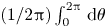$(1/2 {\rm \pi} ) \int _0^{2 {\rm \pi} }\,\textrm {d} \theta$ and ‘$\delta$’ denotes small fast fluctuations around the average; (ii) expand the Hamiltonian $\mathcal {H}$ around ($\bar {X}, \bar {P}$) up to first-order terms in $\delta$; and, finally (iii) take the fast time average of both sides in expressions (3.14) and (3.15), recalling of course that $\overline {\delta X} = \overline {\delta P}= 0$.

After all these steps we arrive at the following set of average equations

(4.2a,b)\begin{equation} \dot{\bar{X}} = \frac{\partial {\mathcal{H}} ({\bar{X}},\bar{P}) } {\partial {\bar{P}}}, \quad \dot{\bar{P}} = -\frac{\partial {\mathcal{H}} (\bar{X},\bar{P}) } {\partial X} + \frac{1}{2}\tau \phi_0^2 \exp\left(\frac{-{2 \bar{X}}^2}{\sigma^2}\right), \end{equation}

that, remarkably, can be canonically derived from the extended Hamiltonian

(4.3)\begin{equation} \tilde{\mathcal{H}} = {\mathcal{H}}-\tau \sigma \varphi_0^2 \frac{\sqrt{2 {\rm \pi}} } {8} \left[1+\textrm{Erf} \left( \sqrt{2}\frac{\bar{X}}{\sigma} \right) \right], \end{equation}

where $\textrm {Erf}$ denotes the Error Function.

Owing to the key fact that $\tilde {\mathcal {H}}$ is conserved, we can use its constant value to establish a link between the initial and final conditions. If particles have enough initial energy to cross the central hump represented by the $\varphi _0$-dependent term present in $\mathcal {H}$, there will be an increase in kinetic energy that reads

(4.4)\begin{equation} {\mathcal{H}}(t \rightarrow +\infty) -{\mathcal{H}} (t =0) = (\sqrt{2{\rm \pi}}/4) \tau \sigma \varphi_0^2 . \end{equation}

As mentioned in the introductory remarks, RR dissipative forces tend to reduce the relative wave–particle velocity, thus accelerating the particles. We also see that the effects of typically small $\tau$ can be magnified by large values of the amplitude $\varphi _0$ and the length $\sigma$.

5. Numerics

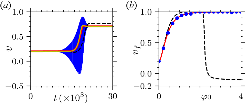
To test and illustrate the theory, let us look at figure 1(a) where we note a nice agreement among the curves obtained from full simulation (based on expressions (2.5), (2.6), (3.2) and (3.3)), its windowed average, and the analytical model (based on expressions (3.6) and (4.2a,b)), all leading to the final velocity $v_f \equiv v(t \rightarrow +\infty ) \sim 0.7$,Footnote ¹ from $v_0 \equiv v(t=0)=0.2$, for $\tau =0.0025$ (soft X-ray band). In all cases discussed in this paper, $x(t=0) = - 4 \sigma$, which is well removed from the wave packet. We point out once again that time dependence of the full original problem and the respective energy variation translate well into an asymmetric non-local effective potential in the average autonomous model. The black line represents the non-canonical approximation $\dot {\bar {X}} = {\bar {P}}/\gamma$ and does not match the simulations and the canonical model.

Figure 1.

$(a)$ Velocity versus time: full simulations in blue, windowed average of full simulations in yellow and the theoretical model in red. We use $\varphi _0=0.5$, $\tau =0.0025$, $v_0\equiv v(t=0)=0.2$ and $\sigma =10^3$. $(b)$ Final velocities versus $\varphi _0$. Solid lines represent the model and symbols represent simulated points. Black lines represent the non-canonical approximation $\dot {\bar {X}}={\bar {P}}/\gamma$.

Expression (4.4) suggests that extreme ejection velocities and energies are obtained when the ‘gain’ parameter $\tau \sigma \varphi _0^2$ becomes much larger than unity.

To examine the issue, figure 1(b) offers a view of the final velocity in terms of the amplitude $\varphi _0$ for $v_0=0.25$. We again take $\sigma =10^3$ and $\tau =0.0025$, so the largest values of $\varphi _0$ in the figure correspond to equally large values of the interaction parameter. From the figure, one can observe that both the fully simulated final velocity and the velocity obtained from the analytical expression (4.4) agree for small values of $\varphi _0$, and both speed up almost simultaneously to $v_f \sim 1$ for large values of the potential. The non-canonical approximation fails for large fields where it predicts reflection whereas the present theory agrees with simulation and predicts acceleration to high levels. One would not observe large accelerations with the non-canonical approach. Reflection is indeed absent for our choice of parameters.

We see a slight discrepancy between analytical and numerical results in figure 1(b) as one closes in on the resonance $v=1$, although the analytical description is very reliable in overall terms. This fact has an effect on energy calculations because energy depends singularly on the precise difference between $v^2$ and unity.

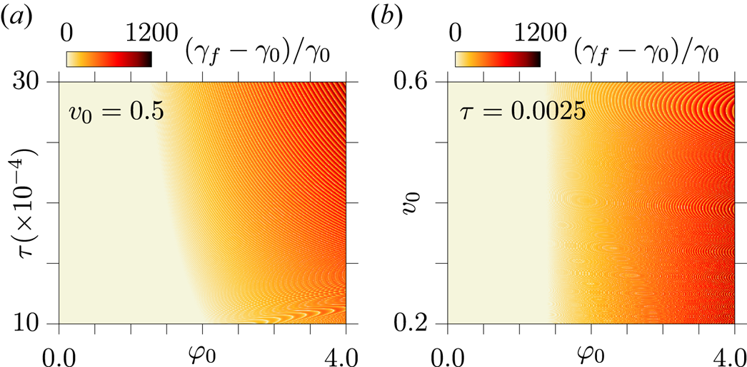
Realizing the need for exact analysis here, in figure 2 we examine a general colour-graded view of the behaviour of numerically simulated normalized gain $(\gamma _f-\gamma _0)/\gamma _0$ as a function of $\varphi _0$ and $\tau$ (in figure 2a), and as a function of $\varphi _0$ and $v_0$ (in figure 2b). The injection velocity does not affect the gain, which is, however, extremely sensitive to $\tau$ and $\varphi _0$. The maximum levels of energy gain in the X-ray band are comparable with what is seen in wake-field accelerators (Welsh et al. Reference Welsh, Wiggins, Issac, Brunetti, Manahan, Islam, Cipiccia, Aniculaesei, Ersfeld and Jaroszynski2012; Kim et al. Reference Kim, Pathak, Pae, Lifschitz, Sylla, Shin, Hojbota, Lee, Sung and Lee2017). The smoother regions of the graphics coincide with the smoother ascending section of figure 1(b) and the high-gain region (with $v \sim 1$) exhibits a semi-periodic pattern resulting from the neighbouring resonance.

Figure 2.

Color-graded plot representing the gain $\Delta \gamma \equiv (\gamma _f-\gamma _0)/\gamma _0$: $v_0=0.5$ in $(a)$ and $\tau =0.0025$ in $(b)$.

6. Electromagnetic effects

This work was aimed at the canonical analysis of RR effects arising in electron dynamics under the action of longitudinal modes. However, before concluding the paper, it is perhaps relevant to have a quick look at the role of electromagnetic effects when the longitudinal mode is replaced by a transverse one. 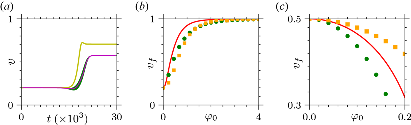The development of the full canonical average formalism of electromagnetic modulated modes is non-trivial and is currently under way; however, the numerical integration of the dynamics of an electron under the action of a modulated plane-polarized wave moving along the $x$-axis, with the electric field pointing along the $y$-axis and the magnetic field pointing along the $z$-axis, can be more straightforwardly obtained. We consider both a stationary modulational envelopeFootnote ² with the same shape as used in expression (3.1) and a moving envelope that propagates at the speed of light. Comparison with the corresponding longitudinal mode analyzed in figure 1 is portrayed in figure 3. One sees that acceleration is somewhat suppressed in the electromagnetic case, although clearly present. Higher amplitudes pull the final velocity towards the speed of light, as previously, even considering the moderate wave amplitudes indicated or the non-stationary envelope. As mentioned previously, the challenge now is to elaborate the canonical averaging formalism for transverse modes, which should reproduce the dependence of the gain factor on the combination $\tau \times (\textrm {field})^2$, already seen in previous works (Piazza Reference Piazza2008; Harvey, Heinzl & Marklund Reference Harvey, Heinzl and Marklund2011).

Figure 3.

$(a)$ Longitudinal velocity versus time: full simulations in green, windowed average for of full simulations assuming the longitudinal (transverse) wave in yellow (magenta). We use $\varphi _0=0.5$, $\tau =0.0025$, $v_0\equiv v(t=0)=0.2$ and $\sigma =10^3$. $(b)$ Final longitudinal velocities versus the field amplitude (we are considering laser and electrostatic modes with the same amplitude, $a_0=\varphi _0$). The solid red line represents the model assuming a longitudinal wave and the symbols are the result from the full simulations assuming a transverse wave with static (green points) and a moving (orange squares) envelope. $(c)$ The same as in $(b)$, but now assuming the laser and the electron beam are contra-propagating with the electron initial velocity equal to $v_0=0.5$.

In general, the present average method works whenever there are two different time scales in the problem. In particular, it can be used to make comparisons with the cases of co- and counter-propagating high-frequency laser pulses and electron beams. We first extend our results to the counter-propagating case, noting that it suffices to start off with particles coming from $x \rightarrow +\infty$ with negative velocities, or simply modify the wave phase from $x-t$ to $x+t$, which would change the signs of our $g_{\textrm {RR}}$ and the corresponding potential correction in (4.3).

Then we can examine our expressions for gain/loss in the face of previous results obtained for the similar schemes of particle acceleration by transverse waves. For our analysis, we first note that $\dot {\gamma }$ can be written both in the forms $\dot {\gamma }=(\textrm {d}\gamma /\textrm {d}x)\dot {x}=v \,\textrm {d}\gamma /\textrm {d}x$ and $\dot {\gamma }=(\textrm {d} \gamma /\textrm {d}p) \dot {p}=v \dot {p}$ for quasi-uniform pulses, wherefrom we have $\textrm {d}\gamma /\textrm {d}x=\dot {p}$. Making use of expression (7) from Smorenburg et al. (Reference Smorenburg, Kamp, Geloni and Luiten2010) or the proper adaptation of expression (3) from Vranic et al. (Reference Vranic, Martins, Vieira, Fonseca and Silva2014), we can promptly show that in regimes of low velocities $| v |\ll 1$, the energy variation in the electromagnetic (EM) case is given by $\Delta \gamma =\pm (\tau a_0^2 \tilde \sigma /2) \gamma _{\textrm {laser}}^2$, respectively, for co- and counter-propagation. Here $a_0$ is the laser field's amplitude, $\gamma _{\textrm {laser}}=\sqrt {1+a_0^2/2}$ is a constant associated with the effective electron mass resulting from the transverse oscillation, and $\tilde {\sigma }$ is the distance covered by the electron while inside the pulse, which is not necessarily equal to the pulse length if the pulse is moving. We then conclude that the electrostatic and electromagnetic models are functionally similar in low-energy regimes, with equivalent roles played by $\varphi _0$ and $a_0$, especially if $a_0 \ll 1$. In contra-propagating higher-energy situations one can approximate the factor $(\gamma - p)^2$ in Smorenburg et al. (Reference Smorenburg, Kamp, Geloni and Luiten2010) by $4 \gamma ^2$ for $p=\gamma v$ with $v \sim -1$, and eventually absorb the factor of $4$ in a new field amplitude $a_0'=2 a_0$, but now the highly varying factor $\gamma ^2$ would alter the functional dependence of the resulting expression (Vranic et al. Reference Vranic, Martins, Vieira, Fonseca and Silva2014).

The results obtained from the full simulations and from theory (4.4) for the electron final velocity when the laser pulse and the electrons beans are propagating in opposite directions are shown in figure 3(c). We investigate low-velocity situations and the figure shows a reduction in the initial electron speed owing to the RR effect. In fact, we chose large enough fields and velocities such that loss effects are apparent, but moderate enough to suggest the similarities between electrostatic and EM cases.

The present work shows that electron acceleration is significant when carrier frequencies lie in the soft X-ray range, a setting that can be obtained by free-electron laser amplifying systems among others (McNeil & Thompson Reference McNeil and Thompson2010; Zhang et al. Reference Zhang, Tajima, Farinella, Shin, Mourou, Wheeler, Taborek, Chen, Dollar and Shen2016). High levels of acceleration produced by lower frequencies more typical of current laser sources can also be obtained, provided one increases the mode amplitude such that the gain factor discussed earlier keeps its magnitude.

Noting that the cutting-edge lasers (Papadopoulos et al. Reference Papadopoulos, Zou, Le Blanc, Chériaux, Georges, Druon, Mennerat, Ramirez, Martin and Fréneaux2016) might present parameters such as $\sigma \approx 200$, $\varphi _0\approx 100$ and $\lambda _0=0.8\ \mathrm {\mu }\textrm {m}$ (such as $\tau =10^{-8}$), then, from (4.4), $|\Delta {\mathcal {H}}|\approx 0.013$, which is not a large variation in the energy. We point out, however, that in cases of localized pulses additional attention should be given to the electron injection velocity or to the envelope length. Both must be large enough to overcome the initial ponderomotive force. Longer pulses, in particular, may significantly increase the energy gain as seen earlier from (4.4).