2.2 DNS data sets of homogenous isotropic turbulence

Eight existing direct numerical simulations of forced homogeneous isotropic turbulence are analysed, in which the Reynolds number based on the Taylor micro-scale $Re_{\unicode[STIX]{x1D706}}$ varies between 34.6 and 1131. The lowest Reynolds numbers ( $Re_{\unicode[STIX]{x1D706}}=34.6$ –177) were computed using the same numerical scheme as in Valente, da Silva & Pinho (Reference Valente, da Silva and Pinho2014). However, we consider a Newtonian fluid instead of the viscoelastic fluids in their paper. The data set at $Re_{\unicode[STIX]{x1D706}}=433$ is from the Johns Hopkins University turbulence database (Li et al. Reference Li, Perlman, Wan, Yang, Meneveau, Burns, Chen, Szalay and Eyink2008). 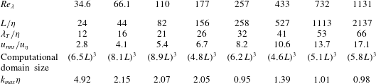Finally, the $Re_{\unicode[STIX]{x1D706}}=257$ , 732 and 1131 cases are from Kaneda et al. (Reference Kaneda, Ishihara, Yokokawa, Itakura and Uno2003), Ishihara et al. (Reference Ishihara, Kaneda, Yokokawa, Itakura and Uno2007). Table 1 provides an overview of the relevant length and velocity scales in these flows. For comparison, in the study of wall-bounded turbulence by Wei et al. (Reference Wei, Elsinga, Brethouwer, Schlatter and Johansson2014) the ratio of the Taylor and Kolmogorov length scales, $\unicode[STIX]{x1D706}_{T}/\unicode[STIX]{x1D702}$ , varied between 20 and 26. The present data extend this range considerably as can be seen from the table.

Table 1.

Overview of length and velocity scales in the DNS data sets, where $L$ is the integral length scale, $\unicode[STIX]{x1D706}_{T}$ is the Taylor length scale, $\unicode[STIX]{x1D702}$ is the Kolmogorov length scale, $u_{rms}$ is the root-mean-square (r.m.s.) velocity and $u_{\unicode[STIX]{x1D702}}$ is the Kolmogorov velocity scale. The maximum wavenumber retained in the simulations is given by $k_{max}$ . The DNS at $Re_{\unicode[STIX]{x1D706}}=34.6$ –177 is from Valente et al. (Reference Valente, da Silva and Pinho2014). The data at $Re_{\unicode[STIX]{x1D706}}=433$ are from Li et al. (Reference Li, Perlman, Wan, Yang, Meneveau, Burns, Chen, Szalay and Eyink2008), while the data at $Re_{\unicode[STIX]{x1D706}}=257$ , 732 and 1131 are from Kaneda et al. (Reference Kaneda, Ishihara, Yokokawa, Itakura and Uno2003), Ishihara et al. (Reference Ishihara, Kaneda, Yokokawa, Itakura and Uno2007).

Figure 1.

Average velocity field in the strain eigenframe for $Re_{\unicode[STIX]{x1D706}}=433$ . The velocity vectors are shown in two cross-planes (a,b). Contours show intensity dissipation (red, corresponding to 30 % of the peak dissipation) and intense swirling strength indicating vortical motion (green, corresponding to 80 % of the peak swirling strength). See Zhou et al. (Reference Zhou, Adrian, Balachandar and Kendall1999) and § 3.3 for the definition of swirling strength. Both the dissipation and the swirling strength are computed from the averaged velocity field.

Figure 2.

Three-dimensional isosurfaces showing intense dissipation (red, 30 % of peak dissipation) and intense swirling strength (green, 80 % of peak swirling strength). $Re_{\unicode[STIX]{x1D706}}=433$ .

2.3 Features of the average flow pattern

The average velocity in the strain eigenframe reveals a shear layer flow structure (figure 1). The plane of the shear layer is at 45 degrees with respect to the $\unicode[STIX]{x1D709}_{1}$ and $\unicode[STIX]{x1D709}_{3}$ axes and contains the $\unicode[STIX]{x1D709}_{2}$ axis. Large-scale regions of nearly uniform flow appear on both sides of the layer. In these regions the flow direction and magnitude change only gradually. However, very strong changes in velocity, hence strong velocity gradients, are associated with the shear layer. This is illustrated by the red contour of intense dissipation (figure 1), which is computed from the averaged velocity field. It shows dissipation is strongest around the origin. The intense dissipation has a sheet-like shape and is associated with a node-saddle flow topology, which is consistent with observations in turbulent flows (Chacin & Cantwell Reference Chacin and Cantwell2000; Moisy & Jimenez Reference Moisy and Jimenez2004; Ganapathisubramani et al. Reference Ganapathisubramani, Lakshminarasimhan and Clemens2008). The intense dissipation sheet is elongated in the direction of the shear layer and thin in the direction perpendicular to the layer. A three-dimensional view is provided in figure 2. Adjacent to the intense dissipation are two intense swirling regions indicated by the green contours (figures 1 and 2), which can be interpreted as vortices. These vortices are also contained within the shear layer. Moreover, they are tube-like as expected (Jimenez et al. Reference Jimenez, Wray, Saffman and Rogallo1993; Ishihara, Gotoh & Kaneda Reference Ishihara, Gotoh and Kaneda2009). The spatial arrangement of vortex tubes next to intense dissipation sheets is again consistent with observations in fully turbulent flow fields (Chacin & Cantwell Reference Chacin and Cantwell2000; Ganapathisubramani et al. Reference Ganapathisubramani, Lakshminarasimhan and Clemens2008). Note that weaker swirling strength regions appear in the curved shear flow outside the layer, but these are below the threshold used for visualization. The same flow features were identified previously in different turbulent flows. Therefore, the average flow pattern in the strain eigenframe is considered universal (Elsinga & Marusic Reference Elsinga and Marusic2010).

We explore the Reynolds number scaling of the various flow features below. Some additional coordinates are introduced in figure 1(a) to facilitate the scaling analysis. In particular, $n$ and $t$ refer to the direction perpendicular and tangential to the shear layer, while $s$ coincides with the $\unicode[STIX]{x1D709}_{2}$ axis. The corresponding velocity components are given by $u_{n}$ , $u_{t}$ and $u_{s}$ , respectively. The scaling analysis of the vortex tubes (§ 3.3) is performed with respect to the location of peak swirling strength along the $t$ axis. Relative to the swirl peak location, new $n_{p}$ and $s_{p}$ axes are defined, which are parallel to the original $n$ and $s$  axes.

3.1 Velocity

The average velocity field in the strain eigenframe is anti-symmetric $(\boldsymbol{u}(\unicode[STIX]{x1D743})=-\boldsymbol{u}(-\unicode[STIX]{x1D743}))$ due to the symmetry of the strain-rate tensor on which it is based. This property has been used in the velocity profiles below to aid convergence. Consequently, only data along the positive axis are presented, as the negative axis is redundant due to the anti-symmetry. Please refer to figure 1(a) for the definition of the different axes.

First, the thickness of the shear layer is assessed using the profiles of tangential velocity, $u_{t}$ , along the shear layer normal direction, $n$ (figure 3). The tangential velocity profiles are normalized by their peak value, $u_{t,max}$ , which is attained at around $n=9\unicode[STIX]{x1D702}$ (figure 3 a). The peak location can be taken as a measure of the thickness of the core of the shear layer, which collapses using the Kolmogorov length scale. The tangential velocity decreases slowly for larger distances from the origin, and reduces to near zero velocity at $n=2.2L$ for $Re_{\unicode[STIX]{x1D706}}>110$ (figure 3 c). The long tail is evidence for the presence of large-scale coherence, i.e. integral-scale motions, adjacent to the shear layer.

The fact that both $\unicode[STIX]{x1D702}$ and $L$ scaling is observed in the tangential velocity profiles is fully consistent with the results of Wei et al. (Reference Wei, Elsinga, Brethouwer, Schlatter and Johansson2014) for wall-bounded turbulence. They also found the peak tangential velocity at $n=9\unicode[STIX]{x1D702}$ and a tail length that scaled on the boundary layer thickness or channel height, which is a macroscopic length scale.

The present tangential velocity profiles cross near $n=1.5\unicode[STIX]{x1D706}_{T}$ (figure 3 b), which marks the transition from the sharp peak to the long tail in the tangential velocity profile. This result is qualitatively similar to results for wall-bounded turbulence (Wei et al. Reference Wei, Elsinga, Brethouwer, Schlatter and Johansson2014), where this crossing is closer to $1\unicode[STIX]{x1D706}_{T}$ . The quantitative difference may be associated with the non-trivial task of defining a Taylor length scale in wall-bounded flow, since the Taylor length evaluated in the streamwise, spanwise or wall-normal directions (or a combination) yield different values. Furthermore, the velocity at the cross-over (at $n=1.5\unicode[STIX]{x1D706}_{T}$ ) appears constant at approximately 45 % of the peak tangential velocity (figure 3 b). This velocity magnitude is consistent with the cross-over velocity in wall-bounded turbulence (at $n=1\unicode[STIX]{x1D706}_{T}$ , Wei et al. Reference Wei, Elsinga, Brethouwer, Schlatter and Johansson2014).

Figure 3.

Tangential velocity profiles along the $n$ axis, which is the direction normal to the shear layer (figure 1 a). The distance to the shear layer centre (i.e. origin) is normalized by the Kolmogorov length scale (a), Taylor length scale (b) and the integral length scale (c). The legend is shown on (d).

It is of interest to consider the Reynolds number scaling of the peak tangential velocity, $u_{t,max}$ , which was used for normalization of the velocity profiles in figure 3. Figure 4 presents $u_{t,max}$ versus the Reynolds number, where the velocity is normalized by the Kolmogorov velocity scale, $u_{\unicode[STIX]{x1D702}}$ , and the r.m.s. velocity, $u_{rms}$ . These velocity scales are associated with the small- and large-scale motions respectively. From the plot it is clear that the peak tangential velocity is constant with Reynolds number when scaled with the Kolmogorov velocity scale. This is somewhat different from the earlier analysis of wall-bounded turbulence (Wei et al. Reference Wei, Elsinga, Brethouwer, Schlatter and Johansson2014), which showed a weak dependence on the small-scale velocity, i.e. the friction velocity. The tangential velocity normalized by the friction velocity changed by just 5 % over the Reynolds number range considered by Wei et al. (Reference Wei, Elsinga, Brethouwer, Schlatter and Johansson2014). The slight difference in scaling behaviour may be due to the flow (wall-bounded versus homogeneous isotropic turbulence) or a low Reynolds number effect in the wall-bounded flow cases. However, the magnitude of the peak tangential velocity is comparable when normalized by the Kolmogorov velocity scale; 2.5–2.6 in the case of wall-bounded turbulence (Wei et al. Reference Wei, Elsinga, Brethouwer, Schlatter and Johansson2014) while it is 2.7–2.8 in case of homogeneous isotropic turbulence (figure 4). The peak velocity normalized by $u_{rms}$ shows a $Re_{\unicode[STIX]{x1D706}}^{-0.5}$ scaling, which is consistent with $u_{t,max}\sim u_{\unicode[STIX]{x1D702}}$ since $u_{rms}/u_{\unicode[STIX]{x1D702}}\sim Re^{0.25}\sim Re_{\unicode[STIX]{x1D706}}^{0.5}$ .

Figure 4.

Reynolds number scaling of the peak tangential velocity along the $n$ axis (figure 3). The lines show the peak velocity normalized by the Kolmogorov velocity scale (red) and the r.m.s. velocity (blue). Trend lines are shown in black.

Figure 5.

Profiles showing the velocity component in the normal direction $u_{n}$ along the shear layer, i.e. along the $t$ axis (figure 1 a). The distance to the origin is normalized by the Kolmogorov length scale (a), the Taylor length scale (b) and the integral length scale (c). The legend is the same as that shown in figure 3(d).

Profiles of the normal velocity component, $u_{n}$ , along the shear layer are presented in figure 5. Similar plots were used in Wei et al. (Reference Wei, Elsinga, Brethouwer, Schlatter and Johansson2014) to infer the distance between the vortices within the shear layer. In their case the core of the vortex was taken as the zero crossing of the velocity profile, where $u_{n}$ changed sign. The present profiles reveal a zero crossing near $t=18{-}25\unicode[STIX]{x1D702}$ only at low Reynolds numbers, that is, for $Re_{\unicode[STIX]{x1D706}}\leqslant 177$ (figure 5 a). At higher Reynolds number the profiles just show a local minimum near $t=35\unicode[STIX]{x1D702}$ , but $u_{n}$ does not change sign. Consequently, the local streamlines do not spiral around a vortex core for $Re_{\unicode[STIX]{x1D706}}\geqslant 257$ , in contrast to the lower Reynolds number results (Elsinga & Marusic Reference Elsinga and Marusic2010; Wei et al. Reference Wei, Elsinga, Brethouwer, Schlatter and Johansson2014). However, the strong drop in $u_{n}$ around $t=15\unicode[STIX]{x1D702}$ is associated with intense swirling strength at all Reynolds numbers, which is indicative of vortical motion (see § 3.3). The present results suggest that with increasing $Re_{\unicode[STIX]{x1D706}}$ the swirling motion weakens relative to the larger-scale straining motion, which causes the zero crossing to disappear. Besides the primary peak at $t=7\unicode[STIX]{x1D702}$ , there appears a secondary maximum in the profiles between $t=70\unicode[STIX]{x1D702}$ and $120\unicode[STIX]{x1D702}$ ( $t=1.5\unicode[STIX]{x1D706}_{T}$ and $3\unicode[STIX]{x1D706}_{T}$ ). Neither the Kolmogorov, the Taylor, nor the integral length scale can collapse the location of this secondary peak (figure 5), which suggests a mixed scaling with contributions from both large and small scales. Nevertheless, at the integral scale, the tail of the profiles is characterized by low velocity magnitude and $u_{n}<0$ (figure 5 c). Furthermore, the peak normal velocity, $u_{n,max}$ scales with the Kolmogorov velocity scale (not shown), similar to $u_{t,max}$ before.

Figure 6.

Profiles showing the velocity component in the direction of the intermediate principal straining, $u_{s}$ , along the corresponding $s$ axis (figure 1 a). The distance to the origin is normalized by the Kolmogorov length scale (a), the Taylor length scale (b) and the integral length scale (c). The legend is the same as that shown in figure 3(d).

Figure 7.

Reynolds number scaling of the peak $u_{s}$ velocity component along the $s$ axis (figure 6). The lines show the peak velocity normalized by the Kolmogorov velocity scale (red) and the r.m.s. velocity (blue). Trend lines are shown in black.

Vorticity within the shear layer is oriented in the direction of the intermediate principal strain rate, which coincides with the $s$ axis as defined in figure 1(a). The corresponding velocity profile is presented in figure 6. Vorticity stretching is evident from the fact that the strain in the $s$ direction is positive, i.e. $\unicode[STIX]{x2202}u_{s}/\unicode[STIX]{x2202}s>0$ near the origin. For $Re_{\unicode[STIX]{x1D706}}>200$ the slopes of the velocity profiles collapse near the origin when scaled with the Kolmogorov length scale (figure 6 a). However, the velocity peak location continuously increases with Reynolds number in Kolmogorov scaling. In Taylor scaling, the peak locations are scattered around $s=2\unicode[STIX]{x1D706}_{T}$ ( $Re_{\unicode[STIX]{x1D706}}>200$ , figure 6 b), which suggests the fluid motions involved in vorticity stretching scale with the Taylor length scale. The peaks are broad ( ${\sim}1\unicode[STIX]{x1D706}_{T}$ based on the points where the velocity reaches 99 % of the peak velocity) resulting in a relatively large uncertainty on the exact peak location, which explains the observed scatter in figure 6(b). The peak velocity, $u_{s,max}$ , reveals a Kolmogorov velocity scaling only for $Re_{\unicode[STIX]{x1D706}}>200$ (figure 7).

In summary, the velocity peaks along the tangential and normal directions scale with the Kolmogorov length and velocity scale, as expected for the intense dissipative straining motions at the centre of the shear layer. However, the velocity peak in the intermediate straining direction scales with the Taylor length scale (figure 6) and the Kolmogorov velocity scale (at large Reynolds numbers, figure 7). Therefore, the scaling of the straining motions is slightly more complex compared to a basic Kolmogorov scaling. Furthermore, the straining motions reveal coherence up to integral scales.

3.2 Dissipation

The average shear layer reveals a sheet-like intense dissipation $\unicode[STIX]{x1D700}$ , which is symmetric around the centre of the shear layer structure ( $\unicode[STIX]{x1D700}(\unicode[STIX]{x1D743})=\unicode[STIX]{x1D700}(-\unicode[STIX]{x1D743})$ ) (figure 1). Note that the dissipation is computed based on the averaged velocity field. The scaling of the dissipation sheet is investigated using normalized dissipation profiles along the same directions as before. Dissipation returns to zero at approximately $10\unicode[STIX]{x1D702}$ along the shear layer normal direction (figure 8 a), which is a measure for the thickness of the dissipation sheet. The total thickness is $20\unicode[STIX]{x1D702}$ due to symmetry. In the other two directions (figure 8 b,c), dissipation drops to near zero at $\pm 30\unicode[STIX]{x1D702}$ , which implies a total length of $60\unicode[STIX]{x1D702}$ . Only the lowest Reynolds number ( $Re_{\unicode[STIX]{x1D706}}=34.6$ ) deviates indicating slightly smaller structure size. These results represent a first statistical scaling analysis of dissipation sheet dimensions. They are however consistent with the largest length scale of the instantaneous dissipation sheets observed in a jet at $Re_{\unicode[STIX]{x1D706}}=150$ (Ganapathisubramani et al. Reference Ganapathisubramani, Lakshminarasimhan and Clemens2008). Overall, the profiles collapse when scaled with the Kolmogorov length scale ( $Re_{\unicode[STIX]{x1D706}}\geqslant 66.1$ , figure 8), which means the dissipation sheet is a small-scale structure, as expected.

Figure 8.

Profiles of dissipation along the $n$  (a),  $t$  (b) and $s$ axes (c). Dissipation is normalized by its peak value. The profiles for different Reynolds numbers collapse when scaled with the Kolmogorov length scale. The legend is the same as that shown in figure 3(d).

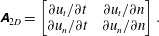
The flow topology associated with the peak dissipation is assessed by decomposing the total shearing at the origin into a contribution from a saddle point topology and a pure layered shear topology (see also Elsinga & Marusic Reference Elsinga and Marusic2010). The decomposition is based on the reduced velocity gradient tensor $\unicode[STIX]{x1D63C}_{2D}$ in the ( $n,t$ ) plane, which takes the form:

(3.1) $$\begin{eqnarray}\unicode[STIX]{x1D63C}_{2D}=\left[\begin{array}{@{}cc@{}}\unicode[STIX]{x2202}u_{t}/\unicode[STIX]{x2202}t\quad & \unicode[STIX]{x2202}u_{t}/\unicode[STIX]{x2202}n\\ \unicode[STIX]{x2202}u_{n}/\unicode[STIX]{x2202}t\quad & \unicode[STIX]{x2202}u_{n}/\unicode[STIX]{x2202}n\end{array}\right].\end{eqnarray}$$

The total shearing is defined as $\unicode[STIX]{x1D70F}_{tot}=(\unicode[STIX]{x2202}u_{t}/\unicode[STIX]{x2202}n+\unicode[STIX]{x2202}u_{n}/\unicode[STIX]{x2202}t)$ , which is the sum of the off-diagonal elements in the reduced strain-rate tensor. Note that $\unicode[STIX]{x2202}u_{t}/\unicode[STIX]{x2202}n>\unicode[STIX]{x2202}u_{n}/\unicode[STIX]{x2202}t>0$ in consequence of the chosen coordinate system (figure 1 a). Then, the total shearing is decomposed into a symmetrical component, $\unicode[STIX]{x1D70F}_{sym}=2\unicode[STIX]{x2202}u_{n}/\unicode[STIX]{x2202}t$ , and an asymmetrical component $\unicode[STIX]{x1D70F}_{asym}=(\unicode[STIX]{x2202}u_{t}/\unicode[STIX]{x2202}n-\unicode[STIX]{x2202}u_{n}/\unicode[STIX]{x2202}t)$ , which is equal to the vorticity. When normalized by the total shearing, these terms correspond to a relative contribution from a pure strain and a layered shear respectively. The results of this analysis are presented in table 2. Most of the total shearing is associated with a shear layer topology ( ${\sim}75\,\%$ ) independent of the Reynolds number, which suggests a link between the vorticity within the shear layer and the core dissipation region. This issue will be further discussed below.

Figure 9.

Profiles of the vorticity component in the direction of the intermediate principal strain, $\unicode[STIX]{x1D714}_{2}$ , taken along the $n$  (a),  $t$  (b) and $s$ axes (c). The profiles for different Reynolds numbers collapse when scaled with the Kolmogorov length scale. The legend is shown in figure 3(d).

Table 2.

The total shearing, $\unicode[STIX]{x1D70F}_{tot}$ , at the origin of the strain eigenframe decomposed into a pure strain, $\unicode[STIX]{x1D70F}_{sym}$ , and a layered shear contribution, $\unicode[STIX]{x1D70F}_{asym}$ .

3.3 Vorticity and swirl

Profiles of the vorticity component in the direction of the intermediate principal strain, $\unicode[STIX]{x1D714}_{2}$ , are shown in figure 9, and reveal a clear collapse in Kolmogorov units. Vorticity changes sign at $n=6\unicode[STIX]{x1D702}$ , which means the thickness of the vorticity layer is $12\unicode[STIX]{x1D702}$ due to symmetry. A minimum in $\unicode[STIX]{x1D714}_{2}$ is found at $n=13\unicode[STIX]{x1D702}$ . Along the shear layer, i.e. the $t$ axis, the $\unicode[STIX]{x1D714}_{2}$ maximum is not at the origin, but is located at $t=6\unicode[STIX]{x1D702}$ . Thus the peak dissipation and the peak vorticity do not coincide, which is consistent with actual turbulence (e.g. Vincent & Meneguzzi Reference Vincent and Meneguzzi1994; Ganapathisubramani et al. Reference Ganapathisubramani, Lakshminarasimhan and Clemens2008). The vorticity magnitude remains significant over larger distances along the shear layer as compared to dissipation (compare figures 8 b and 9 b). The same holds true in the direction of the intermediate principal strain (figures 8 c and 9 c). A characteristic coherence length for shear layer vorticity is $120\unicode[STIX]{x1D702}$ , which is based on the vorticity magnitude reducing to approximately 5 % of its peak value at $60\unicode[STIX]{x1D702}$ distance from the origin in all directions (figure 9) and including symmetry. Similar to the dissipation profiles analysed before, the vorticity profiles at $Re_{\unicode[STIX]{x1D706}}=34.6$ deviate slightly, which is ascribed to insufficient scale separation at low Reynolds number.

The vorticity coherence length along the shear layer, i.e. $120\unicode[STIX]{x1D702}$ , is considerable larger than the commonly reported width of vorticity structures, which varies around 10– $20\unicode[STIX]{x1D702}$ . The reason for the disparity is the azimuthal averaging, which was used when determining the vortex core sizes (e.g. Jimenez et al. Reference Jimenez, Wray, Saffman and Rogallo1993), the vorticity auto-correlation map (Fiscaletti, Westerweel & Elsinga Reference Fiscaletti, Westerweel and Elsinga2014) or the conditionally averaged vorticity field (Mui, Dommermuth & Novikov Reference Mui, Dommermuth and Novikov1996). The vorticity vector defines only a single direction and a perpendicular plane. The two remaining spatial directions within the perpendicular plane are usually arbitrarily defined leading to the azimuthal averaging in that plane, which smears out any shear layer contribution. This effect is illustrated in figure 10, which shows the azimuthal average of shear layer vorticity $\unicode[STIX]{x1D714}_{2}$ in the ( $\unicode[STIX]{x1D709}_{1}$ , $\unicode[STIX]{x1D709}_{3}$ ) plane, i.e. the plane perpendicular to the shear layer vorticity vector. The azimuthal averaging causes the regions of negative and positive $\unicode[STIX]{x1D714}_{2}$ that surround the shear layer to nearly cancel at radial distances greater than $20\unicode[STIX]{x1D702}$ , suggesting the full width of the vorticity structures is only $40\unicode[STIX]{x1D702}$ . Negative $\unicode[STIX]{x1D714}_{2}$ is, for instance, found along the shear layer normal direction (figure 9 a), while positive $\unicode[STIX]{x1D714}_{2}$ is seen along the shear layer (figure 9 b). The resulting vorticity profiles in radial direction are remarkably similar to the vorticity auto-correlation map up to a radial distance of $30\unicode[STIX]{x1D702}$ (figure 10). Only the radial profile for $Re_{\unicode[STIX]{x1D706}}=34.6$ is closer to a Gaussian vorticity distribution, which is typical of a Burgers vortex (Burgers Reference Burgers1948). Therefore, the strain eigenframe is essential in uncovering the nature and the characteristic size of vorticity structures, because it can account for the layer structure and properly defines two directions perpendicular to the vorticity vector.

Figure 10.

Radial profile of vorticity, which is obtained by the azimuthal averaging of $\unicode[STIX]{x1D714}_{2}$ in the ( $\unicode[STIX]{x1D709}_{1}$ , $\unicode[STIX]{x1D709}_{3}$ ) plane. Compared to the profiles in the strain eigenframe (figure 9) vorticity remains coherent over much smaller length scales in the radial profiles. The 10 % threshold is reached at $15\unicode[STIX]{x1D702}$ (compared to $60\unicode[STIX]{x1D702}$ in figure 9 b). The blue symbols ( $+$ ) show a Gaussian distribution with a $7\unicode[STIX]{x1D702}$ radius, while the red symbols (o) show the radial profile from the auto-correlation map of vorticity (data from Fiscaletti et al. Reference Fiscaletti, Westerweel and Elsinga2014).

To isolate vortical motion within the shear layer, we consider the swirling strength as introduced by Zhou et al. (Reference Zhou, Adrian, Balachandar and Kendall1999). The swirling strength is based on an evaluation of the local velocity gradient tensor. If the velocity gradient tensor has a complex eigenvalue pair, the local streamlines describe a spiralling/swirling motion. Then the swirling strength is defined as the absolute value of the imaginary part of the complex eigenvalue pair. In physical terms it represents the angular velocity associated with the swirling motion. In case the velocity gradient tensor has only real eigenvalues, the swirling strength is zero.

Swirling strength is most intense within the shear layer (figure 1) and peaks at $t=11\unicode[STIX]{x1D702}$ (figure 11 b). Hence, the corresponding distance between the two vortices inside the shear layer is $22\unicode[STIX]{x1D702}$ when based on the swirl peak (see also figure 1 a). The present Kolmogorov scaling is different from the Taylor length scaling suggested before when using low Reynolds number data, in which $22\unicode[STIX]{x1D702}$ is of the order of the Taylor length scale (Elsinga & Marusic Reference Elsinga and Marusic2010; Wei et al. Reference Wei, Elsinga, Brethouwer, Schlatter and Johansson2014). The skewed distribution of swirling strength along $t$ is likely due to some variability in the position of the vortex cores relative to the origin of the strain eigenframe. With respect to the swirling strength peak at $t=11\unicode[STIX]{x1D702}$ , new $n_{p}$ and $s_{p}$ axes are defined (figure 1 a). The profile of swirling strength along $n_{p}$ provides the outer diameter of the vortices, which is $18\unicode[STIX]{x1D702}$ (figure 11 a). The vortex core diameter may be defined at the 50 % peak swirling strength cutoff, which is analogue to the Burgers vortex core being defined by the $1/e$ radius of its Gaussian vorticity distribution. By this measure the present core diameter is $11\unicode[STIX]{x1D702}$ , which is close to the commonly reported values for vortex core diameters (6– $10\unicode[STIX]{x1D702}$ , Jimenez et al. Reference Jimenez, Wray, Saffman and Rogallo1993; Ganapathisubramani et al. Reference Ganapathisubramani, Lakshminarasimhan and Clemens2008; Ishihara et al. Reference Ishihara, Gotoh and Kaneda2009). The $s_{p}$ axis coincides with the vortex axis, therefore the swirling strength profile in that direction (figure 11 c) is used to measure the length of the vortex. Based on the zero crossings of the profiles for $Re_{\unicode[STIX]{x1D706}}\geqslant 433$ , the vortex length is determined at $90\unicode[STIX]{x1D702}$ . At lower Reynolds numbers ( $66.1\leqslant Re_{\unicode[STIX]{x1D706}}\leqslant 257$ ) the swirling length profiles reveal longer tails in the $s_{p}$ direction, but the normalized swirling strength in these tails is quite low ( ${<}10\,\%$ , figure 11 c). Therefore, $90\unicode[STIX]{x1D702}$ is considered to be the relevant scale for the vortex length also at lower Reynolds number. This length scale should be interpreted as a coherence length along the vortex axis, because the present averaging process tends to smear out vortical motion that is misaligned with the mean vortex axis. However, the $90\unicode[STIX]{x1D702}$ coherence length compares well with the 60– $100\unicode[STIX]{x1D702}$ characteristic vortex length in visualizations of a jet at $Re_{\unicode[STIX]{x1D706}}=150$ and of high Reynolds number isotropic turbulence (Ishihara et al. Reference Ishihara, Kaneda, Yokokawa, Itakura and Uno2007; Ganapathisubramani et al. Reference Ganapathisubramani, Lakshminarasimhan and Clemens2008). Moreover, the present findings are consistent with Kaneda & Morishita (Reference Kaneda, Morishita, Davidson, Kaneda and Sreenivasan2013), who note that the Reynolds number dependence of the radius of curvature of vorticity lines is similar to that of $\unicode[STIX]{x1D702}$ , rather than that of $\unicode[STIX]{x1D706}_{T}$ .

Both the vorticity and the swirling strength profiles collapse in Kolmogorov length scaling, meaning they are associated with small scales as expected. The present results and the similarity in the visualizations of vortices across Reynolds numbers (Ishihara et al. Reference Ishihara, Kaneda, Yokokawa, Itakura and Uno2007; Ganapathisubramani et al. Reference Ganapathisubramani, Lakshminarasimhan and Clemens2008) suggest that the vortex length is proportional to the Kolmogorov length scale, as opposed to the Taylor length scale (Yamamoto & Hosokawa Reference Yamamoto and Hosokawa1988) or the integral length scale (Jimenez et al. Reference Jimenez, Wray, Saffman and Rogallo1993; Vincent & Meneguzzi Reference Vincent and Meneguzzi1994), which were suggested in the past based on observations in low Reynolds number turbulence.

Figure 11.

Profiles of swirling strength along the $n_{p}$  (a),  $t$  (b) and $s_{p}$ axes (c). Note that the $n_{p}$ and $s_{p}$ axes were defined relative to the swirl peak location long the $t$ axis (see figure 1 a). The profiles for different Reynolds numbers collapse when scaled with the Kolmogorov length scale. The legend is the same as that shown in figure 3(d).

3.4 Local and non-local velocity fields

Further information on the environment of the shear layer is obtained by decomposing the flow into two parts: (i) the velocity induced by shear layer vorticity and (ii) the so-called non-local part. The non-local part is of particular interest and can be interpreted as the shear layer environment. A similar procedure was used before by Hamlington et al. (Reference Hamlington, Schumacher and Dahm2008) in order to define a local and a non-local strain (see also § 4). Here, we take the average velocity field in the strain eigenframe and consider its shear layer vorticity component, $\unicode[STIX]{x1D714}_{2}$ , which induces a flow field according to the Biot–Savart relation:

(3.2) $$\begin{eqnarray}\left.\begin{array}{@{}c@{}}\displaystyle u_{1}(\unicode[STIX]{x1D743})=\frac{1}{4\unicode[STIX]{x03C0}}\int _{\unicode[STIX]{x1D743}^{\prime }}\unicode[STIX]{x1D714}_{2}(\unicode[STIX]{x1D743}^{\prime })\frac{\unicode[STIX]{x1D709}_{3}-\unicode[STIX]{x1D709}_{3}^{\prime }}{|\unicode[STIX]{x1D743}-\unicode[STIX]{x1D743}^{\prime }|^{3}}\,\text{d}^{3}\unicode[STIX]{x1D743}^{\prime },\\ u_{2}(\unicode[STIX]{x1D743})=0,\\ \displaystyle u_{3}(\unicode[STIX]{x1D743})=\frac{-1}{4\unicode[STIX]{x03C0}}\int _{\unicode[STIX]{x1D743}^{\prime }}\unicode[STIX]{x1D714}_{2}(\unicode[STIX]{x1D743}^{\prime })\frac{\unicode[STIX]{x1D709}_{1}-\unicode[STIX]{x1D709}_{1}^{\prime }}{|\unicode[STIX]{x1D743}-\unicode[STIX]{x1D743}^{\prime }|^{3}}\,\text{d}^{3}\unicode[STIX]{x1D743}^{\prime }.\end{array}\right\}\end{eqnarray}$$

The integral is evaluated considering all points $\unicode[STIX]{x1D743}^{\prime }$ where the vorticity magnitude is above a specified threshold. Presently this threshold is set at 5 % of the peak vorticity magnitude. The resulting integration volume corresponds to the ‘intense’ vorticity region associated with the shear layer, which scales with the Kolmogorov length scale and extends up to approximately $60\unicode[STIX]{x1D702}$ distance from the origin in all directions (figure 9). As such, the integration volume is a small scale. The flow computed by (3.2) thus corresponds to the velocity field induced by the shear layer vorticity, $\unicode[STIX]{x1D714}_{2}$ , inside the (small-scale) intense vorticity region. Subtracting the induced velocity from the original flow field in the strain eigenframe yields the non-local flow field.

The induced tangential velocity along the shear layer normal direction, $n$ , is presented in figure 12. For $Re_{\unicode[STIX]{x1D706}}>66.1$ , the induced velocity profiles collapse when normalizing $n$ by the Kolmogorov length scale, $\unicode[STIX]{x1D702}$ , which is expected since the vorticity field, on which it is based, scales with $\unicode[STIX]{x1D702}$ (figure 9). Further note that the velocity normalization is by the peak tangential velocity $u_{t,max}$ of the total flow field in the eigenframe (as in figure 3). Therefore, the induced velocity in figure 12 can be directly compared to the result in figure 3 in order to establish the relative contribution of the induced flow to the total flow. It is observed that the induced flow accounts for ${\sim}70\,\%$ of the peak tangential velocity (figure 12). Consequently, the remaining 30 % is associated with the non-local strain, which is significant. The respective local and non-local contributions appear consistent with the results in table 2, which shows that 75 % of the shearing at the origin is associated with vorticity (local), while the remaining 25 % is due to pure strain (i.e. saddle topology) and does not contain vorticity (non-local).

The non-local tangential velocity profile is obtained by subtracting the induced velocity from the total velocity. It shows a plateau-like region, which extends up to $n=3\unicode[STIX]{x1D706}_{T}$ for $Re_{\unicode[STIX]{x1D706}}\geqslant 257$ (figure 13), where the non-local tangential velocity is around 40 % of the peak total tangential velocity, $u_{t,max}$ . Beyond $n=3\unicode[STIX]{x1D706}_{T}$ the non-local velocity gradually decreases in magnitude. At integral scale, the non-local velocity converges to the total velocity (figure 3 c), because the induced velocity diminishes at large distances from the shear layer (figure 12). Furthermore, small peaks in non-local velocity are observed in the plateau region near $n=60\unicode[STIX]{x1D702}$ , which correspond to a local dip in the induced velocity at the same location (figure 12). They are due to the finite size of the integration volume in the computation of the induced velocity (3.2). Therefore, we do not consider these small peaks significant. In the direction of the intermediate principal strain, $\unicode[STIX]{x1D709}_{2}$ , which coincides with the $s$ axis, the shear layer vorticity does not induce any flow (3.2). Hence, the $u_{s}$ velocity profile (figure 6) represents the total as well as the non-local flow. These profiles reveal a peak at $s=2\unicode[STIX]{x1D706}_{T}$ . Therefore, both non-local velocity profiles (figures 6 and 13) identify the Taylor length, $\unicode[STIX]{x1D706}_{T}$ , as the relevant length scale for the non-local flow. The non-local flow is interpreted as the environment of the shear layer, and contains the motions that stretch vorticity (along the $s$  axis).

Figure 12.

Shear layer vorticity-induced tangential velocity profiles in the direction normal to the shear layer. The induced tangential velocity is normalized by the same peak tangential velocity $u_{t,max}$ used in figure 3. This allows a direct comparison of the induced flow with the profiles obtained from the total flow field in the strain eigenframe (figure 3). The legend is the same as that shown in figure 3(d).

Figure 13.

Non-local tangential velocity profiles in the direction normal to the shear layer, which results from subtracting the shear layer vorticity-induced profile (figure 12) from the total tangential velocity profile (figure 3). Note that figures 3, 12 and the present figure use the same normalization of the tangential velocity. The legend is the same as that shown in figure 3(d).

3.5 Small-scale coherence length and Reynolds number transitions

The vortices and intense dissipation within the present shear layer (figure 2) are independent of the Reynolds number in the sense that both their size and relative positions collapse when scaled with the Kolmogorov length scale (§§ 3.2–3.3). Of course, the instantaneous flow will show a certain variety of small-scale structures, both in sizes and in shapes, but the averaging process in the strain eigenframe identifies the shear layer as statistically relevant. Nevertheless, a comparison with actual turbulence has revealed that the average shear layer structure captures some relevant properties of the underlying turbulent flow, such as; the tube-like shape of the vortices, the sheet-like shape of the dissipation, the fact that intense dissipation is located in between the intense vortices, the alignment of vorticity with the intermediate principal strain, the teardrop shape of the joint-p.d.f. of the invariants of the velocity gradient tensor, and the $k^{-5/3}$ range in the energy spectrum (Elsinga & Marusic Reference Elsinga and Marusic2010, Reference Elsinga and Marusic2016). Therefore, the present average shear layer structure (including the small scales contained within) is considered as a representative, or a characteristic, turbulent flow structure.

The small-scale structure within the average shear layer has a characteristic size of ${\sim}120\unicode[STIX]{x1D702}$ , which is inferred from the shear layer vorticity profiles approaching zero at $\pm 60\unicode[STIX]{x1D702}$ in all directions (figure 9). At that distance from the origin the vorticity magnitude has reduced to approximately 5 % of its peak value. Shear layer vorticity thus remains coherent over that length scale, even if it changes sign in the profile along the $n$ axis (figure 9 a). Note that some features contained within the layer, such as the vortex cores, can be considerably smaller (§ 3.3). However, due to the spatial organization of the vortices and dissipation structures, the small scales in the turbulent flow remain coherent up to ${\sim}120\unicode[STIX]{x1D702}$ . This length scale can be compared with other relevant length scales in the flow, which allows identifying Reynolds number transitions in flow structure.

At very low Reynolds numbers the largest length scale in the flow is comparable to $120\unicode[STIX]{x1D702}$ . In this case, the largest flow scale can be defined as the distance between the points where the tangential velocity returns to zero, which is at $\pm 2.2L$ (figure 3 c). The condition $4.4L>120\unicode[STIX]{x1D702}$ is reached for $Re_{\unicode[STIX]{x1D706}}>45$ (table 1). But even at $Re_{\unicode[STIX]{x1D706}}=110$ , the characteristic small-scale structure and the large scales are poorly separated, and possibly indistinguishable. For example, the kink in the tangential velocity profile at $n=1\unicode[STIX]{x1D706}_{T}-2\unicode[STIX]{x1D706}_{T}$ (figure 3 b), which separates the peak from the tail, is not very pronounced at this Reynolds number. Based on these considerations, a transition in Reynolds number regime may be defined at the point where $L$ is of order $27\unicode[STIX]{x1D702}$ ( $Re_{\unicode[STIX]{x1D706}}\approx 45$ ). Below this Reynolds number developed turbulence cannot exist, since the so-called large scales are smaller in size than the characteristic small-scale structure. Indeed, the present results show that the small-scale structures of dissipation and vorticity are affected at the lowest Reynolds number, $Re_{\unicode[STIX]{x1D706}}=34.6$ . In particular, they are smaller (§§ 3.2 and 3.3) suggesting they are not fully developed.

A second transition in Reynolds number regime is linked to the Taylor length scale, $\unicode[STIX]{x1D706}_{T}$ . In particular, $4\unicode[STIX]{x1D706}_{T}$ represents a characteristic scale for the stretching motions acting in the direction of the small-scale vorticity. This is inferred from the distance between the peaks in the stretching velocity component $u_{s}$ , which are located at $s=\pm 2\unicode[STIX]{x1D706}_{T}$ (figure 6). Moreover, this length scale is associated with the crossing of the tangential velocity profiles (figure 3 b) and the non-local flow (§ 3.4). Only beyond $Re_{\unicode[STIX]{x1D706}}=250$ is $120\unicode[STIX]{x1D702}<4\unicode[STIX]{x1D706}_{T}$ , and a clearer separation between both scales is achieved at $Re_{\unicode[STIX]{x1D706}}\approx 1000$ (table 1). This suggests the possibility of a different flow structure regime. A transition effect at this Reynolds number is evident in the scaling of $u_{s,max}$ , which is the velocity component associated with vorticity stretching (figure 7). It scales with the Kolmogorov velocity scale only when $Re_{\unicode[STIX]{x1D706}}>200$ . Furthermore, the zero crossing of the normal velocity profiles near $t=18{-}25\unicode[STIX]{x1D702}$ (figure 5) disappears for $Re_{\unicode[STIX]{x1D706}}\geqslant 257$ , which is associated with a changing balance between the strength of the local swirling motions and the larger-scale straining motion (§ 3.1). Furthermore, the plateau-like region in the non-local tangential velocity profile extends up to $n=3\unicode[STIX]{x1D706}_{T}$ for $Re_{\unicode[STIX]{x1D706}}\geqslant 257$ (§ 3.4). The mentioned transition effects are related to the development of straining motions, which are associated with the Taylor length scale.

It is of interest to note that the transition at $Re_{\unicode[STIX]{x1D706}}\approx 250$ appears to coincide with the development of a genuine inertial range in the kinetic energy spectra. Compensated energy spectra reveal a true power scaling, close to $k^{-5/3}$ , over a range of wavenumbers, which initially is very narrow at $Re_{\unicode[STIX]{x1D706}}=200$ , but expands with increasing Reynolds number (Yeung & Zhou Reference Yeung and Zhou1997; Kaneda et al. Reference Kaneda, Ishihara, Yokokawa, Itakura and Uno2003; Ishihara et al. Reference Ishihara, Gotoh and Kaneda2009).

The transitions in Reynolds number regime at $Re_{\unicode[STIX]{x1D706}}\approx 45$ and $Re_{\unicode[STIX]{x1D706}}\approx 250$ are gradual though, as is evident from the velocity profiles in § 3.1. Therefore, it is difficult to define sharp bounds for the regimes other than by the considerations given above. The above bounds for the Reynolds number regimes were determined by equating the $120\unicode[STIX]{x1D702}$ size of the characteristic small-scale structure to the characteristic size of the straining motions ( $4\unicode[STIX]{x1D706}_{T}$ ) and the largest flow scale ( $4.4L$ ). One may argue that a proper scale separation is achieved only when $4\unicode[STIX]{x1D706}_{T}$ correspond to some multiple of $120\unicode[STIX]{x1D702}$ . For example, a $4\unicode[STIX]{x1D706}_{T}$ sized straining motion can contain multiple characteristic small-scale structures, when $4\unicode[STIX]{x1D706}_{T}>2\times 120\unicode[STIX]{x1D702}$ , i.e. $\unicode[STIX]{x1D706}_{T}>60\unicode[STIX]{x1D702}$ . This is achieved between $Re_{\unicode[STIX]{x1D706}}=732$ and 1131 (table 1), see also § 3.6.

3.6 Comparison with the high Reynolds number instantaneous shear layer

Shear layers have also been observed in the instantaneous turbulent flow, as mentioned in the introduction. It is, therefore, of interest to compare the present results for the average shear layer in the strain eigenframe with the instantaneous flow and conceptualize the results. The comparison is focused on the significant shear layer observed in high Reynolds number turbulence ( $Re_{\unicode[STIX]{x1D706}}=1131$ ) by Ishihara et al. (Reference Ishihara, Kaneda and Hunt2013), because it is far from the Reynolds number transitions as identified in § 3.5 and there exists a clear scale separation. Moreover, these conditions approach environmental and industrial flows.

The vortical structures in the instantaneous layer were ${\sim}10\unicode[STIX]{x1D702}$ in diameter (Ishihara et al. Reference Ishihara, Kaneda and Hunt2013), which is consistent with the $11\unicode[STIX]{x1D702}$ core diameters in the average layer (§ 3.3). Furthermore, the distance between the vortices is of the same order as the core diameter and scales with the Kolmogorov length scale in both cases. At the same time, integral-scale flow regions bound the shear layers. In the instantaneous flow, the typical distance between the significant layers was of the order of the integral length scale, $L$ (Ishihara et al. Reference Ishihara, Kaneda and Hunt2013). In these $L$ sized regions adjacent to the shear layer, the turbulence was much less intense in terms of the enstrophy and dissipation magnitude when compared to the interior of the shear layer. The average shear layer structure is also bounded by $L$ sized regions, in which the flow conditions are changing only gradually. These regions show in the tangential velocity profiles as long tails, which extend up to $\pm 2.2L$ (figure 3 c). Both the instantaneous and the average shear layer structures, therefore, contain the full range of turbulent length scales, that is, they contain Kolmogorov and integral sized motions simultaneously. Consequently, scale interactions and energy transfer are significant near these layers (Ishihara et al. Reference Ishihara, Kaneda and Hunt2013; Hunt et al. Reference Hunt, Ishihara, Worth and Kaneda2014; Elsinga & Marusic Reference Elsinga and Marusic2016).

The overall thickness of the instantaneous shear layer was ${\sim}4\unicode[STIX]{x1D706}_{T}$ (Ishihara et al. Reference Ishihara, Kaneda and Hunt2013). Conditional averages showed elevated levels of enstrophy and dissipation over the thickness of the layer, which strongly contrasted with the quiescent outer regions. The increase was associated with the numerous intense vortices and dissipation structures clustered within the $4\unicode[STIX]{x1D706}_{T}$ thick layer. In the average shear layer structure, $4\unicode[STIX]{x1D706}_{T}$ is the length scale associated with the non-local strain, which stretches small-scale vorticity and creates the background shear in which the vortices are located (figure 6 and § 3.4). The instantaneous shear layer shows many intense vortices inside the $4\unicode[STIX]{x1D706}_{T}$ layer, while the average shear layer contains only two. A likely explanation for the difference is that the vortices average out in the latter case, which suggests that their relative position in the instantaneous turbulent flow is random beyond a certain distance. This distance is estimated at $120\unicode[STIX]{x1D702}$ , which is the coherence length of the observed characteristic small-scale structure (§ 3.5). At high Reynolds number ( ${\sim}1000$ ) multiple characteristic small-scale structures ( ${\sim}120\unicode[STIX]{x1D702}$ ) fit within a single $4\unicode[STIX]{x1D706}_{T}$ sized straining region. That is, a single straining region can support a number of characteristic small-scale structures by stretching their vorticity, which would explain the observations of Ishihara et al. (Reference Ishihara, Kaneda and Hunt2013). By contrast, only a single characteristic small-scale structure can fit in a $4\unicode[STIX]{x1D706}_{T}$ sized straining region at intermediate Reynolds number ( ${\sim}250$ ). This is schematically represented in figures 14(b) and 14(d).

Figure 14.

Conceptual picture of the instantaneous flow structure in the low (a), intermediate (b,c) and high Reynolds number regime (d,e). At low Reynolds number the integral length scale is comparable to the $120\unicode[STIX]{x1D702}$ size of the characteristic small-scale structure, which consists of two intense swirling motions (green tubes) with an intense dissipation structure in between (red sheet). Consequently, the small-scale structures appear randomly distributed in space (a). At intermediate Reynolds number a $4\unicode[STIX]{x1D706}_{T}$ straining motion (indicated by the grey arrows) can support only a single characteristic small-scale structure of $120\unicode[STIX]{x1D702}$ size (b), whereas at high Reynolds number the same $4\unicode[STIX]{x1D706}_{T}$ straining motion can support multiple characteristic small-scale structures (d). Finally, (c,e) illustrate the arrangement of the $4\unicode[STIX]{x1D706}_{T}$ straining motions and the intense small-scale structures along the edges of the large-scale motions at intermediate and high Reynolds number.

Furthermore, the diagrams in figure 14 illustrate how the shear layer structures are space filling at different Reynolds numbers. At low Reynolds numbers ( $Re_{\unicode[STIX]{x1D706}}\approx 100$ ) the characteristic small-scale structure size is comparable to the integral length scale. Hence, there is effectively only one length scale. As a result, the spacing between neighbouring uncorrelated structures is of similar size as the characteristic small-scale structure itself. The structures, therefore, appear randomly distributed in space (figure 14 a). At $Re_{\unicode[STIX]{x1D706}}\approx 250$ the $4\unicode[STIX]{x1D706}_{T}$ sized straining motions have developed such that they can fully contain a characteristic small-scale structure (figure 14 b). Furthermore, the shear layer structures are bounded by the large-scale motions, which scale with $L$ as discussed above. In the instantaneous flow a single large-scale motion may have several $4\unicode[STIX]{x1D706}_{T}$ sized straining motions distributed along its edges as indicated in figure 14(c). As the Reynolds number increases further, multiple characteristic small-scale structures are contained in each $4\unicode[STIX]{x1D706}_{T}$ sized straining motion (figure 14 d). At the same time, the number of straining motions and small-scale structures along the edges of a large-scale motion increases also (figure 14 e). This leads to a conceptual picture of instantaneous high Reynolds number turbulence, which is consistent with the observations of large significant shear layers separated by $L$ sized quiescent flow regions (Ishihara et al. Reference Ishihara, Kaneda and Hunt2013). We note that vortical and dissipation structures exist in the large-scale quiescent flow regions as well, but they are generally much weaker (Ishihara et al. Reference Ishihara, Kaneda and Hunt2013). The intense vortical and dissipation structures, however, are predominantly located in the straining regions along the edges of the large-scale motions. The difference between the weak and the intense dissipation structures is examined more closely in § 5.

In addition to the spatial structure, we compare the velocity jump across the layers. The maximum velocity difference across the average layer is $0.3u_{rms}$ at $Re_{\unicode[STIX]{x1D706}}=1131$ , which is twice the peak tangential velocity (figure 4) due to the anti-symmetry of the average velocity field. It is clearly lower than the velocity jump across the instantaneous layer (1– $2u_{rms}$ , Ishihara et al. Reference Ishihara, Kaneda and Hunt2013). The instantaneous structure is an example of a strong shear layer, while the averaging also includes weaker structures. We revisit the magnitude of the velocity jump when examining the strong average shear layers, which result from a conditioning on intense dissipation (§ 5).

The fact that the instantaneous and the average shear layer dimensions appear consistent confirms that (i) the instantaneous results are (statistically) relevant and (ii) the averaging in the strain eigenframe yields meaningful results, which capture key features of the instantaneous turbulent flow.