1. Introduction
Polymers have long been recognised as highly effective drag-reducing agents, a discovery first reported by Toms (Reference Toms1948). Despite their significant impact on chemical engineering and marine applications, the underlying mechanism behind polymer-induced turbulent drag reduction remains elusive. In the 1980s, de Gennes proposed the elastic theory, suggesting that stretched polymers can exchange energy with turbulent flows (de Gennes Reference de Gennes1986). This exchange disrupts the energy transfer balance across scales (Frisch Reference Frisch1995). Over the past four decades, numerous studies have explored how polymers affect the energy cascade in bulk turbulence, including theoretical (Sreenivasan & White Reference Sreenivasan and White2000; Fouxon & Lebedev Reference Fouxon and Lebedev2003; Casciola & De Angelis Reference Casciola and De Angelis2007), experimental (Ouellette, Xu & Bodenschatz Reference Ouellette, Xu and Bodenschatz2009; Xi, Bodenschatz & Xu Reference Xi, Bodenschatz and Xu2013; de Chaumont Quitry & Ouellette Reference de Chaumont Quitry and Ouellette2016; Zhang et al. Reference Zhang, Bodenschatz, Xu and Xi2021; Zhang & Xi Reference Zhang and Xi2022; Wang et al. Reference Wang, Zhang and Xi2025a ) and numerical (Benzi et al. Reference Benzi, De Angelis, Govindarajan and Procaccia2003; De Angelis et al. Reference De Angelis, Casciola, Benzi and Piva2005; Kalelkar, Govindarajan & Pandit Reference Kalelkar, Govindarajan and Pandit2005; Perlekar et al. Reference Perlekar, Mitra and Pandit2006, Reference Perlekar, Mitra and Pandit2010; Cai, Li & Zhang Reference Cai, Li and Zhang2010; Watanabe & Gotoh Reference Watanabe and Gotoh2013, Reference Watanabe and Gotoh2014; Valente et al. Reference Valente, Da Silva and Pinho2014, Reference Valente, da Silva and Pinho2016; Nguyen et al. Reference Nguyen, Delache, Simoëns, Bos and El Hajem2016; Fathali & Khoei Reference Fathali and Khoei2019; ur Rehman, Lee & Lee Reference ur Rehman, Lee and Lee2022; Rosti, Perlekar & Mitra Reference Rosti, Perlekar and Mitra2023) works. The violent energy extraction by polymers is reflected in the suppression of the velocity structure functions and emergence of the elastic scaling range, which is between the dissipation range and the inertial range, as displayed in a recent experimental study (Zhang et al. Reference Zhang, Bodenschatz, Xu and Xi2021), and subsequently reproduced numerically (Rosti et al. Reference Rosti, Perlekar and Mitra2023). Despite this progress, there remains an open question regarding how polymers specifically impact turbulent dissipation scales. Notably, there is a scarcity of research exclusively focused on small-scale properties in polymeric turbulence, which constitutes the overarching goal of this paper.
The small-scale properties of turbulent flows can be effectively understood through the velocity gradient tensor (VGT), denoted as
 $A_\textit{ij}\equiv \partial u_i /\partial x_j$
(Meneveau Reference Meneveau2011), where
 $\boldsymbol{u}$
represents the velocity field. The VGT provides valuable insights into fine-scale flow motions. For instance, in incompressible turbulence, the dissipation and production of small scales can be expressed in terms of the second- and third-order moments of
 $\boldsymbol{A}$
, namely its second- and third-order invariants
 $Q \equiv -({1}/{2}) A_\textit{ij}A_\textit{ji}$
and
 $R\equiv -({1}/{3}) A_\textit{ij}A_{jk}A_{ki}$
. As a second-rank tensor,
 $\boldsymbol{A}$
can be naturally decomposed into a symmetric part
 $S_\textit{ij} \equiv (1/2) (A_\textit{ij} + A_\textit{ji} )$
and an antisymmetric part
 $\varOmega _\textit{ij} \equiv ({1}/{2}) (A_\textit{ij} - A_\textit{ji} )$
. Here,
 $\boldsymbol{S}$
and
 $\boldsymbol{\varOmega }$
are also known as the rate-of-strain tensor and the rate-of-rotation tensor, which describe the deformation and rotation motion in turbulent flows, respectively. The latter is related to the vorticity vector
 ${\omega }=\boldsymbol{\nabla } \times \boldsymbol{u}$
through
 $\varOmega _\textit{ij}=-({1}/{2}) \epsilon _\textit{ijk} \omega _k$
, where
 $\epsilon _\textit{ijk}$
is the Levi–Civita symbol. To visualise coherent structures, such as worm-like vortex structures and surrounding dissipation features in Newtonian turbulence, it is helpful to consider the norm of
 $\boldsymbol{S}$
and
 $\boldsymbol{\varOmega }$
, i.e.
 $S_\textit{ij} S_\textit{ij}$
, which is just the dissipation by multiplying the viscosity, and the enstrophy
 $\omega _i \omega _i$
(Kerr Reference Kerr1985; She, Jackson & Orszag Reference She, Jackson and Orszag1990; Ganapathisubramani, Lakshminarasimhan & Clemens Reference Ganapathisubramani, Lakshminarasimhan and Clemens2008; Buaria & Pumir Reference Buaria and Pumir2022). The VGT and related quantities thus have gained popularity for analysing small-scale structures in various turbulent flows, such as wall-bounded flows (Blackburn, Mansour & Cantwell Reference Blackburn, Mansour and Cantwell1996; Chong et al. Reference Chong, Soria, Perry, Chacin, Cantwell and Na1998), isotropic bulk flows (Jiménez et al. 1993; Carter & Coletti Reference Carter and Coletti2018), jet flows (da Silva & Pereira Reference da Silva and Pereira2008; Ganapathisubramani et al. Reference Ganapathisubramani, Lakshminarasimhan and Clemens2008), wake flows (Gomes-Fernandes, Ganapathisubramani & Vassilicos Reference Gomes-Fernandes, Ganapathisubramani and Vassilicos2014; Buxton, Breda & Chen Reference Buxton, Breda and Chen2017) and Rayleigh–Bénard convection flow (Xu, Zhang & Xia Reference Xu, Zhang and Xia2024). Consistent with the K41 theory (Kolmogorov Reference Kolmogorov1941), the small-scale statistics of different types of Newtonian turbulent flows exhibit similar features. In this context, we highlight two relevant features that are closely related to our work. First, there is a preferred alignment of the vorticity vector with the intermediate eigenvector of the rate-of-strain tensor. Second, the joint probability density distributions (PDFs) of the invariants
 $Q$
and
 $R$
, also known as the PDF on the
 $R$
–
 $Q$
map, assume a teardrop shape. These inherent features, as summarised in Meneveau (Reference Meneveau2011), are associated with the rich phenomena of small-scale motions that effectively distinguish turbulent flows from other random velocity fields.
According to the discussions above, it is evident that the impact of polymers on the small scales of turbulence can be assessed by analysing the statistics of the VGT. First, the dissipation
 $S_\textit{ij} S_\textit{ij}$
and enstrophy
 $\omega _i \omega _i$
, representing the magnitude of VGT, are reduced by polymers, and in particular, the reduction in dissipation can be regarded as the drag reduction in bulk turbulence (Kalelkar et al. Reference Kalelkar, Govindarajan and Pandit2005; Perlekar, Mitra & Pandit Reference Perlekar, Mitra and Pandit2006, Reference Perlekar, Mitra and Pandit2010; Cai et al. Reference Cai, Li and Zhang2010). Moreover, the probability distribution of these quantities also contracts after adding polymers, following the same trend as ensemble-averaged values (Liberzon et al. Reference Liberzon, Guala, Lüthi, Kinzelbach and Tsinober2005, Reference Liberzon, Guala, Kinzelbach and Tsinober2006; Cai et al. Reference Cai, Li and Zhang2010; Perlekar et al. Reference Perlekar, Mitra and Pandit2010; Watanabe & Gotoh Reference Watanabe and Gotoh2013; Cocconi et al. Reference Cocconi, De Angelis, Frohnapfel, Baevsky and Liberzon2017; Zhang & Xi Reference Zhang and Xi2022). On the other hand, these distributions for different polymer concentrations collapse when normalised by their standard deviations, suggesting that their functional forms are independent of polymer additives (Watanabe & Gotoh Reference Watanabe and Gotoh2013; Zhang & Xi Reference Zhang and Xi2022). Additionally, by examining the effect of polymers on the
 $R$
–
 $Q$
map, Liberzon et al. (Reference Liberzon, Guala, Kinzelbach and Tsinober2006) found that the typical teardrop shape remains mostly unchanged, except for a reduction in the tail area. A direct numerical simulations (DNS) study by Perlekar et al. (Reference Perlekar, Mitra and Pandit2010) reported observations similar to the experimental results in Liberzon et al. (Reference Liberzon, Guala, Kinzelbach and Tsinober2006). Beyond single-point statistics, polymers also influence the local flow pattern, and the most striking observation is that the vortex filaments are significantly suppressed, leading to much smoother streamlines with weaker velocity gradients (de Chaumont Quitry & Ouellette Reference de Chaumont Quitry and Ouellette2016; Zhang & Xi Reference Zhang and Xi2022; Rosti et al. Reference Rosti, Perlekar and Mitra2023). More precisely, this suppression manifests as a reduction in coherent structures, such as vortex tubes or filaments, particularly when viscoelasticity is enhanced (Bonn et al. Reference Bonn, Couder, Van Dam and Douady1993; Perlekar et al. Reference Perlekar, Mitra and Pandit2006, Reference Perlekar, Mitra and Pandit2010; Cai et al. Reference Cai, Li and Zhang2010; ur Rehman et al. Reference ur Rehman, Lee and Lee2022). Besides, it is also found that additional viscoelasticity can lead to vortex tube structures with increased dimensions (De Angelis et al. Reference De Angelis, Casciola, Benzi and Piva2005), primarily in width compared to length (Watanabe & Gotoh Reference Watanabe and Gotoh2013).
Most studies on small-scale processes in polymeric turbulence rely on numerical simulations, while experimental investigations are relatively rare due to technological constraints. For instance, Bonn et al. (Reference Bonn, Couder, Van Dam and Douady1993) utilised the visibility of bubbles to reveal the suppression of vortex filaments in polymeric turbulence, but no information about the VGT was obtained. Using the particle tracking velocimetry method, Liberzon et al. (Reference Liberzon, Guala, Lüthi, Kinzelbach and Tsinober2005, Reference Liberzon, Guala, Kinzelbach and Tsinober2006) measured the statistics of VGT, but the data points were sparse in space due to the low concentration of tracer particles, which restricted the observations of Eulerian flow structures. In many cases, planar particle image velocimetry (PIV) is commonly employed (Cocconi et al. Reference Cocconi, De Angelis, Frohnapfel, Baevsky and Liberzon2017; Zhang & Xi Reference Zhang and Xi2022), but it provides only two-dimensional velocity information in a plane, which is insufficient for calculating all components of the VGT and for characterising flow structures. To address this gap, our prior work (Wang et al. Reference Wang, Zhang and Xi2025b
) utilised tomographic PIV (Tomo-PIV) to obtain all components of VGT and enable the visualisation of three-dimensional flow structures. Remarkably, most of the experimental and numerical discussions mentioned above are restricted by relatively low Reynolds numbers. Specifically, the Reynolds number based on the Taylor microscale typically does not exceed
 $100$
. These limitations arise mainly due to finite spatial resolution or computational constraints. In our study, we employ the Tomo-PIV method, and provide a dataset with a relatively high Reynolds number, which could further investigate the role of polymers.
In this paper, we study the statistics of VGT in polymeric turbulence in detail. We measure the VGT by the Tomo-PIV method in the bulk of a turbulent von Kármán swirling (VKS) flow. Our Tomo-PIV datasets allow us to reconstruct the three-dimensional Eulerian velocity field with sufficient spatial resolution for calculating all components of the velocity gradients. Focusing on scales dominated by energy dissipation, this study enriches our understanding of how polymers impact the generation of small-scale structures. We present the experimental details, including set-up and data acquisition, in § 2. Section 3 focuses on VGT-based small-scale statistics, and explores their dependence on polymer concentration and turbulent Reynolds number. We will see that in addition to the attenuation of magnitudes, we can observe significant changes in small-scale flow topology, hinting at the presence of vortex sheet structures in polymeric turbulence. To further validate our observations, we provide instantaneous flow visualisations in § 4. Next, in § 5, we present conditional statistics on high enstrophy, which reinforce our findings in the previous sections. Finally, we conclude in § 6 with a summary of our study.
2. Experimental details
The experimental arrangement is the same as in our prior work (Wang et al. Reference Wang, Zhang and Xi2025b ), and here we provide a short but crucial introduction, including the set-up, measurement method, data collection, and definition of parameters. For further details, readers can refer to our previous work (Zhang et al. Reference Zhang, Bodenschatz, Xu and Xi2021; Wang et al. Reference Wang, Zhang and Xi2025a ,Reference Wang, Zhang and Xi b ).
The VKS flow system serves as our turbulence generator, which was dedicated to the study of polymer-laden turbulence with high Reynolds number (Bonn et al. Reference Bonn, Couder, Van Dam and Douady1993; Cadot, Bonn & Douady Reference Cadot, Bonn and Douady1998; Crawford et al. Reference Crawford, Mordant, Xu and Bodenschatz2008; Ouellette et al. Reference Ouellette, Xu and Bodenschatz2009; Xi et al. Reference Xi, Bodenschatz and Xu2013; Burnishev & Steinberg Reference Burnishev and Steinberg2016; de Chaumont Quitry & Ouellette Reference de Chaumont Quitry and Ouellette2016; Sinhuber, Ballouz & Ouellette Reference Sinhuber, Ballouz and Ouellette2018; Zhang et al. Reference Zhang, Bodenschatz, Xu and Xi2021; Zhang & Xi Reference Zhang and Xi2022). The VKS flow is driven by two counter-rotating baffled disks located face-to-face on the base plates at both ends of the closed cylindrical container. The container is 636 mm in height and 480 mm in diameter, with a transparent plexiglass side wall that is 10 mm thick. Seven flat optical windows are mounted on the side wall to facilitate optical measurement, and one of these windows is removable for access inside the container. The disks themselves have radius 110 mm and are equipped with eight vanes, each 50 mm in height, to enhance mixing. These two disks are 416 mm apart, along with the surrounding side walls, creating an area with aspect ratio approximately 1 at the centre of the VKS set-up. Each disk is driven by a 1.5 kW servo motor, allowing for continuous variation of the rotation frequency, denoted as
 $f$
. The working fluid’s temperature is precisely controlled at
 $20\,^\circ{\textrm{C}}$
with minor variation (less than
 $0.1\,^\circ{\textrm{C}}$
) using a refrigerated circulator, and monitored via a PT100 probe inside the container. To achieve the necessary resolution for precise calculation of the VGT, we increased the fluid viscosity by using glycerol. In this study, the Newtonian case denotes the aqueous solution of glycerol with mass fraction 35 %, resulting in viscosity
 $\nu =2.75\times 10^{-6} \ {\textrm{m}}^2\ {\textrm{s}}^{-1}$
. We varied the disk rotation frequency across three cases:
 $f=0.45,0.65,0.85\ \textrm {Hz}$
, allowing us to investigate the Reynolds number (
 $Re$
) dependence, where
 $Re=(2\unicode{x03C0} rf)r/\nu$
.
In the polymeric case, we utilise polyacrylamide (PAM) polymer with average molecular weight
 $M_w=18\times 10^6$
atomic mass units. To prepare the concentrated stock solution of PAM, we followed a method similar to that reported in our previous study (Zhang et al. Reference Zhang, Bodenschatz, Xu and Xi2021). There is an essential difference: instead of using deionised water, we employed the aforementioned aqueous solution of glycerol as the solvent. Subsequently, we slowly added the stock solution containing polymers of a specific quality into the VKS via gravity. Light stirring was carried out before the formal experiments to ensure that the polymer solutions were well mixed yet minimised the physical degradation of PAM. The relaxation time
 $\tau _p$
, which characterises the viscoelasticity of flexible polymer, can be estimated as 115 ms using the Zimm model (Crawford Reference Crawford2004). The polymer concentration
 $\phi$
ranges from 2 to 25 parts per million (ppm) by weight, which falls within the dilute solution regime, where the effects on fluid viscosity can be safely neglected. Also, notice that for polymeric cases with different
 $\phi$
, we still use the parameters of their Newtonian counterparts, such as the Reynolds number, to discriminate these flow fields.
Our objective in this study is to investigate the impact of polymers on bulk turbulence. Consequently, we focus mainly on the flow at the centre of the VKS system, which remains unaffected by side walls. The observation window for the velocity field is measured using the Tomo-PIV method and has size
 $31\times 29\times 6 \,{\textrm{mm}}^{3}$
in the
 $\boldsymbol{e}_x,\boldsymbol{e}_y,\boldsymbol{e}_z$
directions, respectively, where
 $\boldsymbol{e}_y$
denotes the vertical direction (which is the axisymmetric axis of the VKS system), and
 $\boldsymbol{e}_x$
and
 $\boldsymbol{e}_z$
lie in the horizontal plane. Four cameras, two in the horizontal (or equatorial) plane (the
 $\boldsymbol{e}_x O\boldsymbol{e}_z$
plane), and two in the vertical (or meridian) plane (the
 $\boldsymbol{e}_yO \boldsymbol{e}_z$
plane), were arranged at angle
 $30^\circ$
around the
 $\boldsymbol{e}_z$
axis, forming a cross-like configuration (Scarano Reference Scarano2012). Each camera had a 100 mm focal length lens and a 2x extender mounted on the Scheimpflug adapter. The seeding particles used were hollow glass spheres with density
 $\rho _0=1.1\times 10^3 \,{\textrm{kg m}}^{-3}$
and mean diameter
 $d_0=10 \, \unicode{x03BC}{\textrm{m}}$
. These inertialess particles are illuminated by an Nd:YLF laser with wavelength 527 nm. A mirror was used to enhance the intensity and uniformity of the laser beam. Light passing through the optical windows was simultaneously imaged and collected by all four cameras. Calibration involved a two-level target plate and subsequent refinement through volume self-calibration (Wieneke Reference Wieneke2008), achieving a disparity lower than 0.1 pixels. The collected images undergo several processing steps, including image pre-processing, volume reconstruction (using the MART technique), volume cross-correlation and vector post-processing. The final interrogation volumes consisted of 32 voxels on each side, overlapping at 50 %. The vector spacing
 ${\textrm{d}}x$
is thus
 ${\textrm{d}}x=0.55\ \textrm {mm}$
, with
 $57\times 51\times 11$
velocity vectors in the
 $\boldsymbol{e}_x$
,
 $\boldsymbol{e}_y$
and
 $\boldsymbol{e}_z$
directions, respectively. For each case with different
 $Re$
and
 $\phi$
, we collected 3000 snapshots to achieve statistical convergence, with number of statistics approximately
 $10^8$
. All Tomo-PIV procedures mentioned above are executed using DaVis 8.4.0 software.
From the measured velocity field, we have examined the mean flow, which consists of a pumping motion and a shear motion, as reported in previous VKS experiments (Voth et al. Reference Voth, La Porta, Crawford, Alexander and Bodenschatz2002; Debue et al. Reference Debue, Kuzzay, Saw, Daviaud, Dubrulle, Canet, Rossetto and Wschebor2018). Unless otherwise specified, we adopt the fluctuating velocity
 $u_i$
from a classical Reynolds decomposition for data analysis, and refer to it simply as velocity, where
 $i=x,y,z$
corresponds to laboratory coordinates. In addition,
 $\boldsymbol{u}$
exhibits a larger amplitude and better homogeneity than the mean flow, allowing us to use the spatial average to replace the ensemble average. Before doing data analysis, it is crucial to test the volumetric measurement’s accuracy quantitatively. The three velocity components are determined independently, each accompanied by random errors. Therefore, evaluating how well the datasets satisfy the divergence-free condition
 $\partial u_i/\partial x_i=0$
is a valuable test for the accuracy of the measurement (Ganapathisubramani, Lakshminarasimhan & Clemens Reference Ganapathisubramani, Lakshminarasimhan and Clemens2007; Lawson & Dawson Reference Lawson and Dawson2014; Fiscaletti et al. Reference Fiscaletti, Ragni, Overmars, Westerweel and Elsinga2022). The correlation coefficient between
 $-(\partial u_z/\partial z)$
and
 $\partial u_x/\partial x+\partial u_y/\partial y$
is calculated to be approximately 0.8 in all cases, and increases by approximately
 $10\,\%$
after removing the boundary data points that have more significant errors; the details of this method are discussed in our previous work (Wang et al. Reference Wang, Zhang and Xi2025b
). Consequently, we can directly calculate VGT and related quantities from the measured
 $\boldsymbol{u}$
fields, enabling analysis of small-scale information of turbulence with and without polymers.
After conducting thorough qualitative and quantitative assessments, we obtained datasets that allowed us to perform statistical and structural analyses of small-scale turbulence. For these datasets, we use the root mean square of the fluctuating velocity to measure the turbulent characteristic velocity, defined as
 $u^\prime = \langle ({1}/{3}) u_i ({\boldsymbol{x}},t)\, u_i ({\boldsymbol{x}},t) \rangle ^{1/2}$
. Since the flow field is statistically stationary and homogeneous, we employ the temporal and spatial averages in place of the ensemble average, denoted by angle brackets
 $\langle \,\rangle$
. In addition to the aforementioned Reynolds number
 $Re$
based on the geometry of the VKS system, we also use the Reynolds number based on the Taylor microscale, defined as
 $R_\lambda = ( 15u^{\prime 4}/\varepsilon \nu )^{1/2}$
, and these two Reynolds number satisfy the relation
 $R_\lambda \propto \sqrt {Re}$
(Pope Reference Pope2000). Here,
 $\varepsilon =2\nu \langle S_\textit{ij} S_\textit{ij} \rangle$
denotes the mean energy dissipation rate, which along with the viscosity
 $\nu$
characterises the dissipation properties of turbulent flow (Kolmogorov Reference Kolmogorov1941). The Kolmogorov length and time scales are thus defined as
 $\eta =( \nu ^3/\varepsilon )^{1/4}$
and
 $ \tau _\eta = ( \nu /\varepsilon )^{1/2}$
, respectively. For the polymeric case, an additional parameter comes into play: the Weissenberg number
 $\textit{Wi}=\tau _p / \tau _\eta$
, which characterises the relative strength between elastic force and inertial force. Since
 $\tau _p$
remains constant while
 $\tau _\eta$
varies with
 $R_\lambda$
,
 $\textit{Wi}$
is coupled with
 $R_\lambda$
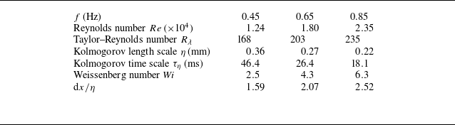
. In table 1, we summarise and list all the parameters mentioned above for our experimental datasets. For all experimental datasets, the values of
 $\textit{Wi}$
are larger than 1 and satisfy Lumley’s time criterion (Lumley Reference Lumley1969), which suggests that the polymer can be stretched by the local flow when the flow responds faster than the polymer. The relative spatial resolution
 ${\textrm{d}}x/\eta$
has order of magnitude 1 and is also included in the table.
Parameters of the experimental datasets in this study.

In our experiments, the Weissenberg number ranges from
 $2.5$
to
 $6.3$
. One might argue that these values are of order unity and close to the critical range for the coil–stretch transition reported by Watanabe & Gotoh (Reference Watanabe and Gotoh2010). However,
 $\textit{Wi}$
in our study is within the range reported in existing literatures on polymeric turbulence (Liberzon et al. Reference Liberzon, Guala, Kinzelbach and Tsinober2006; Ouellette et al. Reference Ouellette, Xu and Bodenschatz2009; Cai et al. Reference Cai, Li and Zhang2010; Perlekar et al. Reference Perlekar, Mitra and Pandit2010; Watanabe & Gotoh Reference Watanabe and Gotoh2013; de Chaumont Quitry & Ouellette Reference de Chaumont Quitry and Ouellette2016). In Watanabe & Gotoh (Reference Watanabe and Gotoh2010), the range
 $\textit{Wi}=3$
–
 $4$
includes the critical coil–stretch transition point, but polymers within this range may still undergo moderate stretching and exert some influence on the flow, albeit weaker than at higher
 $\textit{Wi}$
(Watanabe & Gotoh Reference Watanabe and Gotoh2010). Moreover, Watanabe & Gotoh (Reference Watanabe and Gotoh2010) employed a one-way coupling bead–spring model with a limited number of beads (2 or 20), which may not fully represent the behaviour of the long-chain polymers used in our experiments. The polymers that we used have a high average molecular weight
 $1.8 \times 10^7$
, corresponding to approximately
 $2.5 \times 10^5$
monomers per molecule, which can enhance elastic effects and polymer–flow interactions. Therefore, we expect the polymers to significantly alter the turbulent small-scale statistics under our experimental conditions, even when
 $\textit{Wi}$
is close to the literature-reported critical values (Watanabe & Gotoh Reference Watanabe and Gotoh2010).
3. Statistics of the VGT
In this section, we focus on the statistical properties of VGT
 $\boldsymbol{A}$
, including its invariants, the alignments between vorticity
 $\omega$
and the eigendirections of
 $\boldsymbol{S}$
, and their orientations in the laboratory frame. We will see that our experimental results indicate the existence of vortex sheet structures in polymeric turbulence, which is distinct from its Newtonian counterpart. To begin, we first briefly introduce some definitions and properties of VGT
 $\boldsymbol{A}$
.
The VGT
 $\boldsymbol{A}$
has three invariants,
 $P$
,
 $Q$
and
 $R$
. This work only considers incompressible flows, where the first invariant
 $P=-A_{ii}$
becomes zero due to the incompressible constraint
 $\partial u_i / \partial x_i = 0$
. Consequently, the remaining two invariants,
 $Q \equiv - ({1}/{2}) A_\textit{ij}A_\textit{ji}$
and
 $R\equiv - ({1}/{3}) A_\textit{ij}A_{jk}A_{ki}$
, characterise the structure of the VGT, and each point on the
 $R$
–
 $Q$
map represents a specific local flow pattern. Similarly,
 $\boldsymbol{S}$
and
 $\boldsymbol{\varOmega }$
have their corresponding invariants, of which the non-zero ones are
 $Q_s\equiv -({1}/{2}) S_\textit{ij} S_\textit{ij}$
and
 $R_s \equiv -({1}/{3}) S_\textit{ij} S_{jk} S_{ki}$
for
 $\boldsymbol{S}$
, and
 $Q_\omega \equiv ({1}/{4}) \omega _i \omega _i$
for
 $\boldsymbol{\varOmega }$
. Notice that the dissipation
 $S_\textit{ij} S_\textit{ij}$
and enstrophy
 $\omega _i \omega _i$
mentioned before are actually equivalent to the second-order invariants
 $Q_s$
and
 $Q_\omega$
, respectively, and the third-order invariants, the strain self-amplification
 $R_s$
and the vortex stretching
 $R_\omega \equiv -({1}/{4}) \omega _i S_\textit{ij} \omega _j$
, appear as the nonlinear terms in the equations for
 $Q_s$
and
 $Q_\omega$
(Meneveau Reference Meneveau2011; Johnson & Wilczek Reference Johnson and Wilczek2024). Now noticing that
 $\boldsymbol{A}\equiv \boldsymbol{S}+\boldsymbol{\varOmega }$
, the quantities mentioned above satisfy the relations
 \begin{align} Q &= \frac {1}{4} \left ( \omega _i \omega _i - 2S_\textit{ij} S_\textit{ij} \right ) = Q_\omega + Q_s, \end{align}
 \begin{align} R &= -(1/3) \left ( S_\textit{ij} S_{jk} S_{ki} + (3/4)\omega _i S_\textit{ij} \omega _j \right ) = R_s + R_\omega . \end{align}
Hence we can see that
 $Q$
represents the relative strength between dissipation and enstrophy, while
 $R$
represents the relative strength between strain self-amplification and vortex stretching. These invariants can characterise specific local flow topologies (Soria et al. Reference Soria, Sondergaard, Cantwell, Chong and Perry1994; Blackburn et al. Reference Blackburn, Mansour and Cantwell1996; Meneveau Reference Meneveau2011; Johnson & Wilczek Reference Johnson and Wilczek2024). For instance, the
 $R$
–
 $Q$
map is a typical example, and other maps, such as those between
 $R_s$
and
 $Q_s$
, and between
 $Q_s$
and
 $Q_\omega$
, serve as other examples. We will discuss them in detail in the following text. In particular, the eigenvalues of
 $\boldsymbol{S}$
are defined as
 $\lambda _i$
, and the corresponding eigenvectors as
 $\boldsymbol{e}_i$
, where
 $i=1,2,3$
, and the eigenvalues are ordered as
 $\lambda _1\gt \lambda _2\gt \lambda _3$
. Due to the incompressible condition, we have
 $\lambda _1+\lambda _2+\lambda _3=0$
, thus the extensive eigenvalue satisfies
 $\lambda _1\geqslant 0$
, while the compressive one satisfies
 $\lambda _3 \leqslant 0$
, and the intermediate one,
 $\lambda _2$
, can be either positive or negative. The vortex stretching
 $\omega _i S_\textit{ij}\omega _j$
can be well understood through the alignment of
 $\boldsymbol{\omega }$
with
 $\boldsymbol{e}_i$
, and most studies report that
 $\boldsymbol{\omega }$
tends to align with the intermediate eigenvector
 $\boldsymbol{e}_2$
, instead of the extensive eigenvector
 $\boldsymbol{e}_1$
(Ashurst et al. Reference Ashurst, Kerstein, Kerr and Gibson1987; Elsinga & Marusic Reference Elsinga and Marusic2010; Meneveau Reference Meneveau2011). Furthermore, when the flow satisfies the homogeneity condition, Betchov established that
 $\langle Q \rangle =0$
and
 $\langle R \rangle =0$
(Betchov Reference Betchov1956). Then from (3.1) and (3.2), we have
 $\langle Q_\omega \rangle = -\langle Q_s \rangle$
and
 $\langle R_s \rangle = -\langle R_\omega \rangle$
. It is easy to see that both the enstrophy
 $\langle \omega _i \omega _i \rangle$
and the dissipation
 $\langle S_\textit{ij} S_\textit{ij}\rangle$
are positive as a result of their quadratic forms. The vortex stretching term
 $\langle \omega _i S_\textit{ij} \omega _j \rangle$
is also expected to be positive, as the generation of enstrophy should be positive in turbulent flows. This fact implies that the distribution of vortex stretching should be skewed to the positive part. Moreover, given that
 $\langle R_s \rangle = -\langle R_\omega \rangle = ({1}/{4}) \langle \omega _i S_\textit{ij} \omega _j \rangle = \langle -\lambda _1 \lambda _2 \lambda _3\rangle \geqslant 0$
, we expect that the intermediate eigenvalue
 $\lambda _2$
prefers to be positive statistically (Townsend Reference Townsend1951; Betchov Reference Betchov1956; Meneveau Reference Meneveau2011).
In the following, we will study the invariants associated with
 $\boldsymbol{A}$
as well as
 $\boldsymbol{S}$
and
 $\boldsymbol{\varOmega }$
to explore the impact of polymers on the generation and destruction of small-scale motions in turbulence. We begin by examining their ensemble averages and PDFs in §§ 3.1 and 3.2. Next, in § 3.3, we focus on the local flow topology, characterised by the joint PDFs of the aforementioned invariants, and the statistics of eigenvalues and eigenvectors of
 $\boldsymbol{S}$
are studied in § 3.4. We will find that the statistics are closely related to the vortex sheet structures. Furthermore, our results reveal that the small-scale quantities in VKS are not isotropic, which is discussed in detail in § 3.5. Finally, in § 3.6, we summarise the key findings of the previous subsections, and point out that the observed statistical properties of VGT could be well described by a simple picture: the vortex sheet structures aligned with the axisymmetric axis of the VKS system.
3.1. Ensemble average of invariants
We first examine the impact of polymers on the ensemble-averaged values of invariants appeared in (3.1) and (3.2), namely
 $\langle Q_s \rangle$
,
 $\langle Q_\omega \rangle$
,
 $\langle R_s \rangle$
and
 $\langle R_\omega \rangle$
. We use the
 $R_\lambda = 203$
case here. In figure 1(a), we plot the second-order moments
 $\langle Q_s \rangle$
and
 $\langle Q_\omega \rangle$
, and one can see that their magnitudes decrease significantly as the polymer concentration
 $\phi$
increases, which is consistent with previous studies (De Angelis et al. Reference De Angelis, Casciola, Benzi and Piva2005; Liberzon et al. Reference Liberzon, Guala, Lüthi, Kinzelbach and Tsinober2005, Reference Liberzon, Guala, Kinzelbach and Tsinober2006; Cai et al. Reference Cai, Li and Zhang2010). The well-known suppression of the energy cascade in the inertial range due to polymer additions (Ouellette et al. Reference Ouellette, Xu and Bodenschatz2009; Xi et al. Reference Xi, Bodenschatz and Xu2013; Zhang et al. Reference Zhang, Bodenschatz, Xu and Xi2021) explains the observed reduction in
 $-\langle Q_s \rangle$
and
 $\langle Q_\omega \rangle$
. Furthermore, given the definition of mean energy dissipation rate
 $\varepsilon = 2\nu \langle S_\textit{ij} S_\textit{ij} \rangle$
, the results shown in figure 1(a) can be interpreted as drag reduction in bulk turbulence, as reported by previous DNS studies (Perlekar et al. Reference Perlekar, Mitra and Pandit2006, Reference Perlekar, Mitra and Pandit2010; Cai et al. Reference Cai, Li and Zhang2010). In figure 1(b), we plot the ensemble-averaged third-order quantities, strain self-amplification
 $\langle R_s \rangle$
and vortex stretching
 $\langle R_\omega \rangle$
. Similar to the second-order moments, they also decrease significantly with increasing
 $\phi$
. This is consistent with our intuition that the depression of third-order moments leads to the depression of the small scales in polymeric turbulence (Liberzon et al. Reference Liberzon, Guala, Lüthi, Kinzelbach and Tsinober2005, Reference Liberzon, Guala, Kinzelbach and Tsinober2006; Cocconi et al. Reference Cocconi, De Angelis, Frohnapfel, Baevsky and Liberzon2017), given that the nonlinear third-order terms contribute to the generation of the turbulent system. The insets of figure 1(a,b) show the ratios
 $-\langle Q_s \rangle / \langle Q_\omega \rangle$
and
 $-\langle R_s \rangle / \langle R_\omega \rangle$
, respectively. Remarkably, the data points remain close to 1 within the considered concentration range, which validates the homogeneity condition discussed above (Betchov Reference Betchov1956), i.e. the fluctuation velocity field could be treated as locally homogeneous, allowing spatial averages to replace ensemble averages. We also notice that some DNS studies introduced the concept of polymer stress, and found that while the nonlinear generation terms are suppressed, the polymer stress terms sustain the small scales of turbulence (Cai et al. Reference Cai, Li and Zhang2010; Watanabe & Gotoh Reference Watanabe and Gotoh2014; ur Rehman et al. Reference ur Rehman, Lee and Lee2022), but due to technical limitations, our current experimental set-up cannot precisely quantify the impact of polymers on turbulent dynamics.
The ensemble-averaged invariants as functions of
 $\phi$
: (a) second-order moments
 $\langle Q_s \rangle$
and
 $\langle Q_\omega \rangle$
; (b) third-order moments
 $\langle R_s \rangle$
and
 $\langle R_\omega \rangle$
. Insets show the ratios between two second- or third-order moments. (c) The skewness of
 $\boldsymbol{S}$
,
 $\langle R_s \rangle / (-\langle Q_s \rangle )^{3/2}$
. In (a–c), we use the
 $R_\lambda =203$
dataset. (d) Plot of
 $\langle Q_s \rangle$
normalised by the corresponding Newtonian values (
 $\phi =0$
) for three Reynolds numbers,
 $R_\lambda = 168,203,235$
.

For the rate-of-strain tensor
 $\boldsymbol{S}$
, we have discussed its second- and third-order moments,
 $\langle Q_s \rangle$
and
 $\langle R_s \rangle$
. Both of these moments are significantly suppressed with increasing polymer concentration
 $\phi$
. In addition, figure 1(c) plots the skewness of
 $\boldsymbol{S}$
,
 $\langle R_s \rangle / (-\langle Q_s \rangle )^{3/2}$
, as a function of
 $\phi$
. Within the considered range of
 $\phi$
, the skewness consistently maintains a non-zero value, indicating a skewed distribution of
 $R_s$
(Sreenivasan & Antonia Reference Sreenivasan and Antonia1997; Meneveau Reference Meneveau2011) as we mentioned before. However, as
 $\phi$
increases, the skewness gradually decreases. Consequently, we conclude that polymers not only reduce the magnitude of the second- and third-order moments of
 $\boldsymbol{S}$
(or
 $\boldsymbol{A}$
), but also weaken its skewed distribution, as will be further demonstrated through the PDFs of invariants in the next subsection.
In figure 1(d), we further explore the Reynolds number effect on the moments of VGT in polymeric turbulence; as an example, we plot
 $\langle Q_s \rangle$
normalised by its corresponding Newtonian value for various
 $R_\lambda$
(and also
 $\textit{Wi}$
). We observe that the normalised
 $\langle Q_s \rangle$
decreases differently as a function of polymer concentration
 $\phi$
. Specifically, both curves exhibit a rapid descent at a particular
 $\phi$
value, and as
 $R_\lambda$
increases, this descent occurs at higher polymer concentration. On the other hand, at sufficiently high
 $\phi$
, the results for all three
 $R_\lambda$
seem to level off to almost the same extent. Experimental work in VKS with baffled disks (Ouellette et al. Reference Ouellette, Xu and Bodenschatz2009) and smooth disks (Zhang & Xi Reference Zhang and Xi2022) also reported a similar phenomenon. Recall that a reduction in the amplitude of
 $\langle Q_s \rangle$
or
 $\langle Q_\omega \rangle$
corresponds to a drag reduction; the results in figure 1(d) as well as previous VKS experiments may represent a maximum drag reduction, suggesting a balanced energy exchange between polymers and turbulent flows.
3.2. The PDFs of invariants
Compared to the ensemble average, PDFs provide more comprehensive information about physical quantities. Figure 2 illustrates the PDFs of
 $- Q_s$
and
 $ Q_\omega$
at
 $R_\lambda =203$
. Consistent with the reduction of mean value shown in figure 1(a), all the PDF curves in figure 2 contract as polymer concentration
 $\phi$
increases. Intense events with high dissipation or enstrophy are significantly suppressed, which has been shown in extensive experimental (Liberzon et al. Reference Liberzon, Guala, Lüthi, Kinzelbach and Tsinober2005, Reference Liberzon, Guala, Kinzelbach and Tsinober2006; Zhang & Xi Reference Zhang and Xi2022) and numerical (Perlekar et al. Reference Perlekar, Mitra and Pandit2010; Watanabe & Gotoh Reference Watanabe and Gotoh2013; Cocconi et al. Reference Cocconi, De Angelis, Frohnapfel, Baevsky and Liberzon2017; ur Rehman et al. Reference ur Rehman, Lee and Lee2022) research. In addition, we can see that although the mean values of
 $Q_s$
and
 $Q_\omega$
balance each other (
 $- \langle Q_s \rangle = \langle Q_\omega \rangle$
), the tails of the PDFs of
 $Q_\omega$
are always broader than the tails of
 $Q_s$
for different
 $\phi$
, which is consistent with the Newtonian cases (Buaria & Pumir Reference Buaria and Pumir2022; Gotoh, Watanabe & Saito Reference Gotoh, Watanabe and Saito2023).
In the insets of figure 2(a,b), we demonstrate that these PDFs exhibit similar functional forms across different polymer concentrations when normalised by their respective standard deviations. This observation is qualitatively consistent with previous experimental and numerical studies (Perlekar et al. Reference Perlekar, Mitra and Pandit2010; Watanabe & Gotoh Reference Watanabe and Gotoh2013; Zhang & Xi Reference Zhang and Xi2022). Upon closer examination, we find that this collapse is particularly good within approximately ten standard deviations, i.e. in the core region of the PDFs. In contrast, the tails exhibit some scatter, which may arise from limited statistical convergence. Alternatively, the observed differences in the tails could reflect a physical effect: the presence of polymers may alter the occurrence and distribution of extreme dissipation events, which are often associated with coherent flow structures. As is shown later, our results indicate that polymer additives cause significant changes in these flow structures, which could lead to the observed modification of the PDF tails for
 $-Q_s$
and
 $Q_\omega$
. Slight tail deviations have also been reported in previous studies (Perlekar et al. Reference Perlekar, Mitra and Pandit2010; Watanabe & Gotoh Reference Watanabe and Gotoh2013; Zhang & Xi Reference Zhang and Xi2022), and our findings offer a possible physical explanation for this phenomenon.
PDFs of (a)
 $- Q_s$
and (b)
 $ Q_\omega$
for different concentrations
 $\phi$
. The insets show the same PDF curves but normalised by their corresponding standard deviations
 $\sigma$
. Here, we use the
 $R_\lambda =203$
dataset.

Next, we present the PDFs of third-order invariants
 $R_s$
and
 $-R_\omega$
in figure 3. In figure 3(a,c), the PDF curves exhibit a clear trend of shrinking as
 $\phi$
increases, consistent with the reduction of ensemble average shown in figure 1(b). Similar to the PDFs of
 $- Q_s$
and
 $ Q_\omega$
shown in figure 2, the third-order quantities are also significantly depressed by the polymer additives, as reported in previous studies (Liberzon et al. Reference Liberzon, Guala, Lüthi, Kinzelbach and Tsinober2005, Reference Liberzon, Guala, Kinzelbach and Tsinober2006; Cai et al. Reference Cai, Li and Zhang2010; Cocconi et al. Reference Cocconi, De Angelis, Frohnapfel, Baevsky and Liberzon2017; ur Rehman et al. Reference ur Rehman, Lee and Lee2022). Notably, both
 $R_s$
and
 $-R_\omega$
are positively skewed, which remains consistent in polymeric turbulence. And this skewness plays a crucial role in the turbulent energy transfer process. In the context of decaying homogeneous isotropic turbulence, Cai et al. (Reference Cai, Li and Zhang2010) analysed the changes in production terms, and concluded that polymer addition reduces the strength of vortex stretching, leading to the drag-reducing phenomenon.
The PDFs of (a)
 $R_s$
and (c)
 $-R_\omega$
for different polymer concentrations
 $\phi$
. (b,d) The PDFs using the same data as in (a,c), but normalised by their corresponding standard deviations, and the curves of higher
 $\phi$
have been shifted downwards by
 $10^{0.6}$
relative to their lower-value neighbours, for clarity. The insets show the original, unshifted data. These results are based on the
 $R_\lambda =203$
dataset.

In figure 3(b,d), we present the same data as in figure 3(a,c), but normalised by their own standard deviations. Note that in the insets, the normalised PDF curves with different
 $\phi$
exhibit similar forms. However, upon closer examination, we observe that right-branch (positive values) curves, representing a positive generation of enstrophy, decrease more rapidly with increasing
 $\phi$
than left-branch curves (negative values). In the main plots of figure 3(b,d), these curves for different
 $\phi$
have been uniformly shifted down
 $10^{0.6}$
equidistant from each other for clearer comparisons. An interesting finding is that the asymmetric distribution of
 $R_s$
or
 $-R_\omega$
is suppressed by polymers, resulting in a decreased value of skewness, which is consistent with figure 1(c). Cocconi et al. (Reference Cocconi, De Angelis, Frohnapfel, Baevsky and Liberzon2017) first noticed that polymer additions have a stronger depressive effect on the positive values of vortex stretching
 $\omega _i S_\textit{ij} \omega _j$
than on the negative parts. Subsequently, ur Rehman et al. (Reference ur Rehman, Lee and Lee2022) studied the orientation between vorticity
 $\omega _i$
and
 $S_\textit{ij} \omega _j$
. They found that the probability of parallel alignment between these vectors decreases, while the probability of their being antiparallel increases, which favours negative values of vortex stretching
 $\omega _i S_\textit{ij} \omega _j$
. Our current experiments yield results similar to those shown in figure 9(a) of ur Rehman et al. (Reference ur Rehman, Lee and Lee2022) (not shown for simplicity). In summary, polymers suppress intense events of the third-order moments of the VGT, with a more substantial impact on positive values of vortex stretching. Our experimental results at higher Reynolds numbers are fully consistent with previous findings at lower Reynolds numbers.
Joint PDFs of (a–d)
 $Q$
and
 $R$
, (e–h)
 $Q_s$
and
 $R_s$
, (i–l)
 $Q_s$
and
 $Q_\omega$
, non-dimensionalised by the second-order moment
 $\langle Q_\omega \rangle$
. The values of the PDF contours are logarithmic, and are
 $0.01,0.1,1$
in (a–d),
 $0.005, 0.05,0.5$
in (e–h), and
 $0.01,0.1,1$
in (i–l). Results are for (a,e,i) the Newtonian case, (b, f, j)
 $\phi =5\,{\textrm{ppm}}$
, (c,g,k)
 $\phi =10\,{\textrm{ppm}}$
, (d,h,l)
 $\phi =25\,{\textrm{ppm}}$
. Black curves correspond to the
 $R_\lambda =203$
case, and (d,h,l) also provide the results from another two Reynolds numbers with
 $\phi =25\,{\textrm{ppm}}$
.

3.3. Local flow topology
In addition to basic statistics such as ensemble averages and PDFs, the impact of polymers on small-scale turbulence can be further investigated through the local flow topology, which could be characterised by the invariants introduced earlier in this section. In figure 4, we present joint PDFs of these invariants, which often exhibit universal features across various turbulent flows. The joint PDFs of
 $Q$
and
 $R$
,
 $Q_s$
and
 $R_s$
,
 $Q_s$
and
 $Q_\omega$
are shown in the left, middle and right columns of the figure, respectively. The first row corresponds to the Newtonian case, while the three rows below show the polymeric cases with polymer concentrations
 $\phi = 5$
,
 $10$
and
 $25\,{\textrm{ppm}}$
, respectively, to better illustrate the concentration dependence of the results. The black curves correspond to
 $R_\lambda =203$
, and in order to clarify the Reynolds number dependence, we also include the
 $\phi =25\,{\textrm{ppm}}$
case for two additional Reynolds numbers in figure 4(d,h,l).
In figure 4(a–d), we show the joint PDFs between
 $Q$
and
 $R$
, non-dimensionalised by
 $\langle Q_\omega \rangle$
. Contours with values
 $0.01,0.1,1$
have been selected. The Vieillefosse tails denoted by
 $D \equiv ({27}/{4}) R^2+Q^3 = 0$
are also shown in figure 4, where
 $D$
represents the discriminant of the characteristic equation of
 $\boldsymbol{A}$
. The different regions in this
 $R$
–
 $Q$
map characterise the local flow topology: the
 $D\gt 0, R\lt 0$
and
 $D\gt 0, R\gt 0$
regions correspond to local vortex stretching and vortex compression, respectively, while the
 $D\lt 0, R\lt 0$
and
 $D\lt 0, R\gt 0$
regions correspond to deformation motion subjected to uniaxial extension and biaxial extension, respectively (Vieillefosse Reference Vieillefosse1982, Reference Vieillefosse1984; Cantwell Reference Cantwell1992; Meneveau Reference Meneveau2011). As shown in figure 4(a) for the Newtonian case, one can easily recognise the teardrop shape of the PDF, which is consistent with previous experimental results (Gomes-Fernandes et al. Reference Gomes-Fernandes, Ganapathisubramani and Vassilicos2014; Buxton et al. Reference Buxton, Breda and Chen2017; Fiscaletti et al. Reference Fiscaletti, Ragni, Overmars, Westerweel and Elsinga2022; Warwaruk & Ghaemi Reference Warwaruk and Ghaemi2024). This teardrop shape of the PDF on the
 $R$
–
 $Q$
map is believed to be a universal phenomenon for small scales in turbulent flows (Elsinga & Marusic Reference Elsinga and Marusic2010; Meneveau Reference Meneveau2011).
However, after adding polymers, one can clearly see that the contours in figure 4(b–d) shrink in the
 $R$
direction, contrasting with the Newtonian case. Furthermore, as
 $\phi$
increases, the degree of shrinkage becomes more pronounced. This attenuation of
 $R$
indicates the suppression of dissipation and enstrophy generation, consistent with previous discussions on the depression of mean values and PDFs of
 $R_s$
and
 $R_\omega$
. Interestingly, our findings here are significantly different from previous results reported by Liberzon et al. (Reference Liberzon, Guala, Kinzelbach and Tsinober2006) and Perlekar et al. (Reference Perlekar, Mitra and Pandit2010). They observed that the teardrop shape still exists on the
 $R$
–
 $Q$
map for polymeric turbulence, albeit reduced in area. These differences may arise from the relatively small Reynolds numbers and Weissenberg numbers in the literature. A low Reynolds number implies underdeveloped turbulence, while a low Weissenberg number indicates that the flow is not vigorous enough to effectively stretch polymer molecules, leading to limited polymer–turbulence interactions.
This dramatic change of
 $R$
–
 $Q$
PDFs might be understood by the polymer dynamics in turbulent flow. It is expected that the coiled polymer molecule can be stretched by the flow into long chain structures (White & Mungal Reference White and Mungal2008), as clearly shown by a number of numerical simulations (Terrapon et al. Reference Terrapon, Dubief, Moin, Shaqfeh and Lele2004; Peters & Schumacher Reference Peters and Schumacher2007; Watanabe & Gotoh Reference Watanabe and Gotoh2010). In Watanabe & Gotoh (Reference Watanabe and Gotoh2010), by plotting the polymer extension conditioned on the different regions of the
 $R$
–
 $Q$
map, they reported that the longest polymer or maximum extension is found preferentially in the upper left or lower right regions. These regions correspond to extreme vortex stretching or biaxial extension motion, where polymers experience significant stretching. Analogous to a dumbbell spring, once stretched, the polymer may dampen the flow, especially in these specific regions. We also notice that people have suggested the interaction between polymer and near-wall vortices as an explanation of turbulent drag reduction (Dubief et al. Reference Dubief, White, Terrapon, Shaqfeh, Moin and Lele2004), and indeed, people observed depression of the VGT, especially
 $R$
in polymeric wall turbulence (Mortimer & Fairweather Reference Mortimer and Fairweather2022; Warwaruk & Ghaemi Reference Warwaruk and Ghaemi2024), which might be a relevant phenomenon for our findings here in bulk turbulence.
In figure 4(e–h), we present the joint PDFs of the non-dimensionalised invariants of
 $\boldsymbol{S}$
,
 $Q_s$
and
 $R_s$
, with contour values
 $0.005, 0.05,0.5$
. Since the rate-of-strain tensor
 $\boldsymbol{S}$
is real and symmetric, the PDFs should lie below the curve defined by
 $D_s \equiv ({27}/{4}) R_s^2+Q_s^3$
, i.e.
 $D_s$
should be less than
 $0$
, where
 $D_s$
denotes the discriminant of the characteristic equation of
 $\boldsymbol{S}$
. In reality, a few events with
 $D_s\gt 0$
arise due to unavoidable divergence errors in the experiments, which can also be seen in previous experimental results (Gomes-Fernandes et al. Reference Gomes-Fernandes, Ganapathisubramani and Vassilicos2014; Warwaruk & Ghaemi Reference Warwaruk and Ghaemi2024). These events are rare (approximately 1 % of overall single-point statistics) and do not significantly impact our conclusions. In general, this joint PDF of
 $Q_s$
and
 $R_s$
characterises the local topology of deformation motion, and given that
 $R_s = -\lambda _1 \lambda _2 \lambda _3$
in incompressible flows,
 $R_s$
also marks the sign of
 $\lambda _2$
. In the Newtonian case shown in figure 4(e), the contours are inclined to the right-hand dashed line with
 $D_s=0, R_s\gt 0$
, which corresponds to
 $\lambda _1 : \lambda _2 : \lambda _3 = 1:1:-2$
. This result is consistent with the previous finding in the literature that the ratios
 $\lambda _1 : \lambda _2 : \lambda _3 = 3:1:-4$
or
 $2:1:-3$
are most probable (Ashurst et al. Reference Ashurst, Kerstein, Kerr and Gibson1987; Soria et al. Reference Soria, Sondergaard, Cantwell, Chong and Perry1994; Blackburn et al. Reference Blackburn, Mansour and Cantwell1996), suggesting a geometry of biaxial stretching. However, in the polymeric case shown in figure 4( f–h), the contours gradually approach the vertical dashed line as
 $\phi$
increases, corresponding to two-dimensional stretching with
 $\lambda _1 : \lambda _2 : \lambda _3 = 1:0:-1$
. This is consistent with the results shown in figures 3(b) and 4(b–d), since the third-order invariant
 $R_s$
vanishes in this two-dimensional structure.
Next, in figure 4(i–l), we examine the joint PDFs of
 $Q_s$
and
 $Q_\omega$
, which characterise the flow topology associated with energy dissipation. We have chosen contour values
 $0.01$
,
 $0.1$
and
 $1$
. In the Newtonian case shown in figure 4(i), the PDF concentrates towards the horizontal axis. This region represents the event with strong enstrophy but weaker dissipation, corresponding to a vortex tube structure (Soria et al. Reference Soria, Sondergaard, Cantwell, Chong and Perry1994; da Silva & Pereira Reference da Silva and Pereira2008). Surprisingly, when polymers are added, the PDF shape changes dramatically, as shown in figure 4( j–l), where we observe that the PDF increasingly concentrates along the diagonal line as the polymer concentration increases. This region represents the events with comparable strength between enstrophy and dissipation, corresponding to vortex sheet structures (Soria et al. Reference Soria, Sondergaard, Cantwell, Chong and Perry1994).
Combining the results in figure 4, we can conclude that the local flow topology in polymeric turbulence differs significantly from the Newtonian case. The local flow patterns of vortex stretching and biaxial extension, which are abundant in Newtonian fluid turbulence and essential for the stretching of polymer molecules, are greatly suppressed. Furthermore, as the concentration increases, this suppression effect exhibits a nearly continuous trend and becomes progressively stronger. Additionally, figure 4 exhibits statistical characteristics resembling a vortex sheet structure with two-dimensional properties, which has not been reported in other studies. Finally, results with different
 $R_\lambda$
in figure 4(d,h,l) demonstrate that these findings become more pronounced as
 $R_\lambda$
increases.
3.4. Statistics related to eigenvalues and eigenvectors of the rate-of-strain tensor
The joint PDFs of
 $Q_s$
and
 $R_s$
shown in figure 4(h) suggest that the two-dimensional strain structure, indicated by the ratios
 $\lambda _1 : \lambda _2 : \lambda _3 = 1 : 0 : -1$
, dominates the statistics of the rate-of-strain tensor
 $\boldsymbol{S}$
in polymeric turbulence. In this subsection, we further investigate the statistics related to the eigenframe of
 $\boldsymbol{S}$
and its dependence on concentration
 $\phi$
. Notice that the PDFs of
 $\lambda _1$
,
 $\lambda _2$
and
 $\lambda _3$
all shrink significantly with increasing
 $\phi$
, similar to the trend of invariants shown in § 3.2, which are not shown here for simplicity. We introduce the relative magnitudes of
 $\lambda _1$
and
 $\lambda _2$
, defined as
 $\lambda _1^\ast \equiv \sqrt {6}\,\lambda _1 / \sqrt {\lambda _1^2 + \lambda _2^2 + \lambda _3^2}$
and
 $\lambda _2^\ast \equiv \sqrt {6}\,\lambda _2 / \sqrt {\lambda _1^2 + \lambda _2^2 + \lambda _3^2}$
, and present the PDFs of
 $\lambda _1^\ast$
and
 $\lambda _2^\ast$
for different values of
 $\phi$
in figure 5(a,b), respectively. For the Newtonian case represented by the blue line marked with a cross symbol, we observe that the PDF of
 $\lambda _1^\ast$
peaks at approximately 1.5 and is nearly symmetric, while the distribution of
 $\lambda _2^\ast$
is asymmetric with a peak value at approximately
 $\lambda _2^\ast = 0.5$
, consistent with previous studies (Ashurst et al. Reference Ashurst, Kerstein, Kerr and Gibson1987; Lund & Rogers Reference Lund and Rogers1994; Ganapathisubramani et al. Reference Ganapathisubramani, Lakshminarasimhan and Clemens2008; Buaria, Bodenschatz & Pumir Reference Buaria, Bodenschatz and Pumir2020). It is worth noting that our measured VGTs do not fully satisfy the divergence-free condition, which affects the ranges of values in figure 5. Ideally, incompressible flows should yield values within the ranges
 $\lambda _1^\ast \in [1,2]$
and
 $\lambda _2^\ast \in [-1,1]$
.
On the other hand, when polymers are added to the flow, the PDFs of
 $\lambda _1^\ast$
and
 $\lambda _2^\ast$
both change. Figure 5(a) shows that as
 $\phi$
increases, the peak becomes more pronounced and shifts towards
 $\sqrt {3}$
, indicated by the vertical dashed line. Meanwhile, in figure 5(b), the PDF of
 $\lambda _2^\ast$
gradually becomes symmetric with respect to
 $\lambda _2^\ast = 0$
, which is consistent with previous numerical studies on bulk turbulence with polymers (Perlekar et al. Reference Perlekar, Mitra and Pandit2010; Cocconi et al. Reference Cocconi, De Angelis, Frohnapfel, Baevsky and Liberzon2017). With increasing concentrations, we clearly see that the PDFs in figure 5 become contracted, with their peaks increasing and converging toward a certain value. Actually, the changes of the PDFs of
 $\lambda _1^\ast$
and
 $\lambda _2^\ast$
are mutually consistent, corresponding to the dominance of the eigenvalue distribution
 $\lambda _1 : \lambda _2 : \lambda _3 = 1 : 0 : -1$
, due to
 $\lambda _1 + \lambda _2 + \lambda _3 = 0$
, as we already observed in figure 4(h). Additionally, Liberzon et al. (Reference Liberzon, Guala, Lüthi, Kinzelbach and Tsinober2005) and Cocconi et al. (Reference Cocconi, De Angelis, Frohnapfel, Baevsky and Liberzon2017) listed the ensemble averages of these three eigenvalues in bulk turbulence with and without polymers, which is also consistent with our findings here.
The PDFs of (a) the normalised extensive eigenvalue
 $\lambda _1^\ast \equiv \sqrt {6}\,\lambda _1 / \sqrt {\lambda _1^2 + \lambda _2^2 + \lambda _3^2}$
and (b) the normalised intermediate eigenvalue
 $\lambda _2^\ast =\sqrt {6}\,\lambda _2/\sqrt {\lambda _1^2+\lambda _2^2+\lambda _3^2}$
of
 $\boldsymbol{S}$
for different values of
 $\phi$
. Notice that our measured VGTs do not fully satisfy the divergence-free condition. Thus the values of
 $\lambda _1^\ast$
and
 $\lambda _2^\ast$
do not completely fall in the ranges
 $[1,2]$
and
 $[-1,1]$
, respectively, satisfied by incompressible flows. Dataset
 $R_\lambda =203$
is used here.

Apart from the eigenvalues
 $\lambda _i$
of
 $\boldsymbol{S}$
, the statistics of their corresponding eigenvectors
 $\boldsymbol{e}_i$
are also of interest, especially their alignments with the vorticity vector
 $\boldsymbol{\omega }$
(Elsinga & Marusic Reference Elsinga and Marusic2010; Meneveau Reference Meneveau2011). It is well known that in Newtonian turbulence, the vorticity vector has a preferential alignment with the intermediate eigenvector
 $\boldsymbol{e}_2$
(Ashurst et al. Reference Ashurst, Kerstein, Kerr and Gibson1987; Meneveau Reference Meneveau2011), which is also observed in our experiments. In figure 6, we plot the PDFs of
 $\vert {\cos (\boldsymbol{\omega }, \boldsymbol{e}_i)}\vert$
for different concentrations
 $\phi$
, and in figure 6(b), the Newtonian result indicated by the blue lines marked with cross symbols clearly shows a pronounced peak at
 $\vert {\cos (\boldsymbol{\omega }, \boldsymbol{e}_2)}\vert =1$
. Additionally, the tendency for vorticity to be randomly aligned with the extensive eigenvector (resulting in a flat PDF for
 $\vert {\cos (\boldsymbol{\omega }, \boldsymbol{e}_1)}\vert$
) and perpendicular to the compressive one (with peaks at
 $\vert {\cos (\boldsymbol{\omega }, \boldsymbol{e}_3)}\vert =0$
) can also be observed in figure 6(a,c), respectively.
Alignment of the vorticity vector
 $\boldsymbol{\omega }$
with the (a) first (
 $\boldsymbol{e}_1$
), (b) second (
 $\boldsymbol{e}_2$
) and (c) third (
 $\boldsymbol{e}_3$
) eigenvectors of
 $\boldsymbol{S}$
, for different values of
 $\phi$
. Dataset
 $R_\lambda =203$
is used here.

Now we move on to the discussions for polymeric turbulence, and we can see from figure 6 that as the concentration
 $\phi$
increases, the preferential alignment of
 $\boldsymbol{\omega }$
with
 $\boldsymbol{e}_2$
becomes more pronounced, and the peak value of the PDF curve also increases. At the same time, the vorticity vector tends to be orthogonal to
 $\boldsymbol{e}_1$
and
 $\boldsymbol{e}_3$
, with a more significant change observed for
 $\boldsymbol{e}_1$
. At the highest concentration
 $\phi =25\,{\textrm{ppm}}$
considered here, the PDFs of
 $\vert {\cos (\boldsymbol{\omega }, \boldsymbol{e}_1)}\vert$
and
 $\vert {\cos (\boldsymbol{\omega }, \boldsymbol{e}_3)}\vert$
are nearly identical, indicating an axisymmetric configuration of vorticity in the eigenframe of strain. Our findings here differ from previous DNS studies, where it was reported that adding polymers has little impact on the alignment between the vorticity and the eigenvectors of the strain tensor
 $\boldsymbol{S}$
(Watanabe & Gotoh Reference Watanabe and Gotoh2010; Cocconi et al. Reference Cocconi, De Angelis, Frohnapfel, Baevsky and Liberzon2017; ur Rehman et al. Reference ur Rehman, Lee and Lee2022). It is possible that the inconsistency between our experimental results and previous DNS studies is related to the large-scale structure. In the current experiments conducted in VKS, the configuration satisfies only the axisymmetry condition rather than isotropy. We will discuss the effect of large-scale anisotropy in detail in the next subsection.
3.5. Enhanced small-scale anisotropy
In the preceding subsections, we explored the statistics of invariants related to the VGT and the eigenframe of
 $\boldsymbol{S}$
. Now, in this subsection, we move to the discussions on the impact of large-scale effects on VGT statistics, with a particular focus on the influence of large-scale anisotropy. In real fluid systems, such as wall flows and free-shear flows, large-scale motions are inherently anisotropic. Adding polymers to the flow further amplifies this anisotropy. For instance, in boundary layers, the streamwise velocity fluctuation increases with polymer addition, while the transverse fluctuation decreases (Warholic, Massah & Hanratty Reference Warholic, Massah and Hanratty1999; White, Somandepalli & Mungal Reference White, Somandepalli and Mungal2004). Therefore, the anisotropy becomes more pronounced compared to the Newtonian counterpart. Similar observations have been made in other flow systems as well (Tong et al. Reference Tong, Goldburg, Huang and Witten1990; van Doorn, White & Sreenivasan Reference van Doorn, White and Sreenivasan1999; Boffetta et al. Reference Boffetta, Mazzino, Musacchio and Vozella2010; Lacassagne et al. Reference Lacassagne, Simoëns, El Hajem, Lyon and Champagne2019; Lin, Owolabi & Lin Reference Lin, Owolabi and Lin2022; Peng, Zhang & Xi Reference Peng, Zhang and Xi2023; Wang et al. Reference Wang, Zhang and Xi2025a
; Xu et al. Reference Xu, Liu, Li and Xia2025). In systems with finite Reynolds numbers, the anisotropy of large-scale motions has a substantial influence on small-scale quantities like the VGT, resulting in directional dependence in its statistical properties. The VKS system employed in our study is also anisotropic, satisfying only the axisymmetric condition. As a result, statistical differences arise between the axial and horizontal directions (La Porta et al. Reference La Porta, Voth, Crawford, Alexander and Bodenschatz2001; Voth et al. Reference Voth, La Porta, Crawford, Alexander and Bodenschatz2002; Ouellette et al. Reference Ouellette, Xu, Bourgoin and Bodenschatz2006). An intriguing and crucial question then emerges: how does the presence of polymers affect the anisotropy of the VKS flow, particularly the properties of the VGT that we investigate in this work?
The anisotropy of the VGT can be characterised by the orientation of the vorticity vector
 $\boldsymbol{\omega }$
and the eigenvectors
 $\boldsymbol{e}_i$
(
 $i=1,2,3$
) of
 $\boldsymbol{S}$
in the laboratory frame. We denoted the unit vectors of laboratory coordinates as
 $\boldsymbol{e}_x$
,
 $\boldsymbol{e}_y$
and
 $\boldsymbol{e}_z$
. In figures 7 and 8, we plot the statistics of alignments between vorticity and eigenvectors of strain with respect to the laboratory coordinates for different polymer concentrations. Let us begin by examining the Newtonian case, represented by the blue lines marked with cross symbols. In an ideal isotropic system, the vectors
 $\boldsymbol{\omega }$
and
 $\boldsymbol{e}_i$
(
 $i=1,2,3$
) should not exhibit any preferential alignment with the laboratory axes
 $\boldsymbol{e}_a$
(
 $a=x,y,z$
). But from figure 7, we can see that the vorticity vector
 $\boldsymbol{\omega }$
and the intermediate eigenvector
 $\boldsymbol{e}_2$
tend to align weakly with the vertical direction
 $\boldsymbol{e}_y$
, while
 $\boldsymbol{e}_1$
and
 $\boldsymbol{e}_3$
show a weak tendency to be perpendicular to
 $\boldsymbol{e}_y$
. We notice that all the results shown in figures 7 and 8 exhibit symmetry between
 $\boldsymbol{e}_x$
and
 $\boldsymbol{e}_z$
, consistent with the axisymmetric nature of the VKS flows. Our findings here agree with the previous experimental measurements (Zimmermann et al. Reference Zimmermann, Xu, Gasteuil, Bourgoin, Volk, Pinton and Bodenschatz2010), revealing subtle yet observable anisotropy in the VGT in Newtonian von Kármán turbulence.
Alignments of the vorticity vector
 $\boldsymbol{\omega }$
with the laboratory coordinates
 $\boldsymbol{e}_a$
(
 $a=x,y,z$
) for different concentrations
 $\phi$
. Dataset
 $R_\lambda =203$
is used here.

Alignments of the three eigenvectors
 $\boldsymbol{e}_i$
(
 $i=1,2,3$
) of
 $\boldsymbol{S}$
with the laboratory coordinates
 $\boldsymbol{e}_a$
(
 $a=x,y,z$
) for different
 $\phi$
. Dataset
 $R_\lambda =203$
is used here.

When polymers are introduced, figures 7 and 8 show that the trend of alignment gradually strengthens with increasing polymer concentration. Specifically, at the highest concentration
 $\phi =25\,{\textrm{ppm}}$
,
 $\boldsymbol{\omega }$
and
 $\boldsymbol{e}_2$
strongly aligns with
 $\boldsymbol{e}_y$
, while
 $\boldsymbol{e}_1$
and
 $\boldsymbol{e}_3$
prefer to be perpendicular to
 $\boldsymbol{e}_y$
and lie in the
 $\boldsymbol{e}_x O\boldsymbol{e}_z$
plane. Still, the statistics at all values of
 $\phi$
exhibit symmetry between
 $\boldsymbol{e}_x$
and
 $\boldsymbol{e}_z$
. We can clearly see a pronounced enhancement of small-scale anisotropy due to polymer additions. Furthermore, the turbulent energy cascade is known for erasing anisotropy from large scales through inter-scale energy transfer within the inertial range (Frisch Reference Frisch1995), and as the Reynolds number increases, small-scale statistics tend towards isotropy. However, in our study, despite increasing the Reynolds number from
 $168$
to
 $235$
(not shown in the figures), we do not observe this trend when polymers are added. This suggests that the enhancement of small-scale anisotropy may be linked to the suppression of energy cascades caused by polymer additions.
In such an anisotropic flow system, several open questions arise. The first is that, in addition to small-scale local shear, large-scale shear may also act to stretch the polymer molecules. In the centre region of the VKS flow, the turbulent fluctuation is much stronger than the mean velocity field, suggesting that polymers are primarily elongated by the turbulent flow. In our previous work (Wang et al. Reference Wang, Zhang and Xi2025b ), we observed that polymers do not substantially alter the mean flow pattern – i.e. the pumping and shearing motions characteristic of the VKS flow remain largely unchanged. However, polymers do reduce the intensity of large-scale flows while increasing their characteristic length and time scales, effectively weakening large-scale shear. Within the limited measurement volume considered in the present study (approximately 3 cm near the centre of the VKS set-up), these results suggest that large-scale flows may have a limited ability to stretch polymer molecules. That said, we cannot fully exclude the potential influence of large-scale shear in polymeric turbulence. This important question will be addressed in future work, which will entail larger measurement volumes, broader parameter ranges, and alternative experimental configurations.
Another natural question is: does the orientation of polymer molecules have a preferred direction? This issue has been extensively discussed in previous studies (Den Toonder et al. Reference Den Toonder, Hulsen, Kuiken and Nieuwstadt1997; van Doorn et al. Reference van Doorn, White and Sreenivasan1999; Lacassagne et al. Reference Lacassagne, Simoëns, El Hajem, Lyon and Champagne2019; Peng et al. Reference Peng, Zhang and Xi2023) and confirmed through DNS studies (Guimarães et al. Reference Guimarães, Pimentel, Pinho and da Silva2020; Mortimer & Fairweather Reference Mortimer and Fairweather2022). Even in the case of homogeneous isotropic turbulence without a mean flow, observations indicate that polymers tend to be perpendicular to the eigenvector
 $\boldsymbol{e}_3$
, and prefer to align with
 $\boldsymbol{e}_2$
at high
 $\textit{Wi}$
(Watanabe & Gotoh Reference Watanabe and Gotoh2010; Valente, Da Silva & Pinho Reference Valente, Da Silva and Pinho2014; ur Rehman et al. Reference ur Rehman, Lee and Lee2022). Given these findings, it seems plausible that polymers also exhibit a preferred orientation in VKS flows, namely, along the axial direction. This preferential orientation, in turn, modifies the local flow topology and further enhances the anisotropy. Similar observations of polymer-induced small-scale anisotropy have been reported in previous studies (Crawford et al. Reference Crawford, Mordant, Xu and Bodenschatz2008; Boffetta et al. Reference Boffetta, Mazzino, Musacchio and Vozella2010; Vonlanthen & Monkewitz Reference Vonlanthen and Monkewitz2013; Wang et al. Reference Wang, Zhang and Xi2025b
). Moreover, several works have suggested that the alignment of polymer molecules is influenced by local flow topology (Watanabe & Gotoh Reference Watanabe and Gotoh2010; Valente et al. Reference Valente, Da Silva and Pinho2014; ur Rehman et al. Reference ur Rehman, Lee and Lee2022), and is often oriented along the mean flow direction (Guimarães et al. Reference Guimarães, Pimentel, Pinho and da Silva2020; Mortimer & Fairweather Reference Mortimer and Fairweather2022). However, the mechanism by which oriented polymers enhance existing anisotropy remains a topic for further theoretical exploration, which would inevitably improve our understanding of drag-reducing for wall flows when polymers are present.
3.6. Vortex sheet structures
We have already seen that in a turbulent VKS flow, polymers have strong effects on the statistics of the VGT. Recall the results in figures 4–8; some of them are consistent with previous studies, and some are quite different. To provide a plausible explanation for our findings, let us summarise the key observations for polymeric VKS turbulence.
-
(i) Attenuation of the third-order statistics (such as
 $R$
or
$R_s$
; see figure 4
b,d).
-
(ii) The ratios between strain eigenvalues tend to be
$ \lambda _1 : \lambda _2 : \lambda _3 = 1:0:-1$
(see figures 4
d and 5). -
(iii) The coexistence of dissipation
$Q_s$
and enstrophy
$Q_\omega$
with similar strength (see figure 4
f). -
(iv) The vorticity vector
$\boldsymbol{\omega }$
aligns preferentially with
$\boldsymbol{e}_2$
and is perpendicular to both
$\boldsymbol{e}_1$
and
$\boldsymbol{e}_3$
(see figure 6). -
(v) The preferential alignment of
$\boldsymbol{\omega }$
and
$\boldsymbol{e}_2$
with the aixal direction
$\boldsymbol{e}_y$
, and the symmetry between
$\boldsymbol{e}_x$
and
$\boldsymbol{e}_z$
in all statistics (see figures 7 and 8).


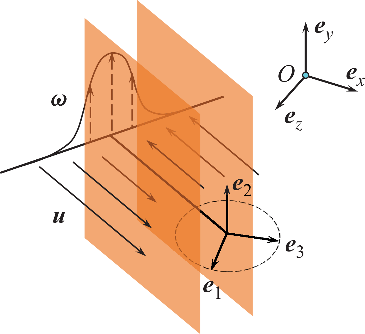
Surprisingly, we find that a vortex sheet model, like the Burgers vortex layer solution for the Navier–Stokes equations, can perfectly explain results (i)–(iv) listed above. We sketch the Burgers vortex sheet solution (see e.g. equation 5 in Andreotti Reference Andreotti1997) in figure 9, where it becomes evident that the Burgers layer corresponds to a simple shear structure. In a simple local shear flow, it is well established that the magnitudes of the second-order invariants
 $Q_s$
and
 $Q_\omega$
are equal to each other, and the third-order invariants
 $R_s$
and
 $R_\omega$
vanish. Furthermore, the intermediate eigenvector of strain,
 $\boldsymbol{e}_2$
, aligns with the vorticity vector, and the ratios between strain eigenvalues are precisely given by
 $ \lambda _1 : \lambda _2 : \lambda _3 = 1:0:-1$
. The observation (v) can be attributed to the vortex layer being extended along the
 $\boldsymbol{e}_y$
axis and randomly orientated in the local horizontal plane, as depicted in figure 9. In this case,
 $\boldsymbol{\omega }$
and
 $\boldsymbol{e}_2$
point towards
 $\boldsymbol{e}_y$
, while
 $\boldsymbol{e}_1$
and
 $\boldsymbol{e}_3$
randomly orientate in the
 $\boldsymbol{e}_x O \boldsymbol{e}_z$
plane.
Sketch illustrating the vortex sheet structure, where
 $\boldsymbol{u}$
denotes the velocity field,
 $\boldsymbol{\omega }$
is the vorticity, and
 $\boldsymbol{e}_{i}$
(
 $i=1,2,3$
) are the eigenvectors of
 $\boldsymbol{S}$
. The laboratory coordinates are denoted by orthogonal axes
 $\boldsymbol{e}_{a}$
(
 $a=x,y,z$
). Notice that the orientation of
 $\boldsymbol{e}_{1}$
(and thus
 $ \boldsymbol{e}_{3}$
) is random within the
 $\boldsymbol{e}_{x} O \boldsymbol{e}_{z}$
plane, as depicted by the dashed circle. This figure is inspired by figure 1(b) of Andreotti (Reference Andreotti1997).

In summary, we have discovered that the single-point statistics of the VGT in polymeric turbulence can be well described by the local vortex sheet structure, which has not been reported previously. Our experimental results exhibit differences compared with the existing literature, which finds that with polymer additions, the shape of
 $R$
–
 $Q$
PDFs is qualitatively unchanged (Liberzon et al. Reference Liberzon, Guala, Kinzelbach and Tsinober2006; Perlekar et al. Reference Perlekar, Mitra and Pandit2010), and there are no significant differences for vorticity alignment with eigendirections of
 $\boldsymbol{S}$
from Newtonian fluids (Watanabe & Gotoh Reference Watanabe and Gotoh2010; Cocconi et al. Reference Cocconi, De Angelis, Frohnapfel, Baevsky and Liberzon2017; ur Rehman et al. Reference ur Rehman, Lee and Lee2022). This discrepancy may be attributed to the intrinsic anisotropy present in VKS flow, which is absent in the numerical simulations. In this section, we focus solely on single-point statistics. In the subsequent two sections, by investigating the instantaneous visualisation and conditional statistics on vorticity, we will try to identify the flow structures and explore their relation with our proposed model in figure 9.
4. Structural visualisation
The previous section explored the impact of polymers on the statistics of small-scale turbulence, represented by the VGT and related quantities. These statistics are closely related to the local flow topology (see (3.1) and (3.2)), as discussed in § 3.3. Additionally, figure 4 revealed a typical type of flow pattern characterised by the emergence of vortex sheet structures. The aim of the present section is to further investigate the changes in small-scale flow topology after adding polymers by visualising the flow structures. Specifically, we continue to use
 $-Q_s$
(representing dissipation) and
 $Q_\omega$
(representing enstrophy) to reveal the flow structures, which have been extensively adopted in turbulence research (Ganapathisubramani et al. Reference Ganapathisubramani, Lakshminarasimhan and Clemens2008; Gomes-Fernandes et al. Reference Gomes-Fernandes, Ganapathisubramani and Vassilicos2014; Buaria & Pumir Reference Buaria and Pumir2022). We present instantaneous results from a selected snapshot. While this selected snapshot contains more representative coherent structures, it is not fundamentally distinct from the other snapshots.
A representative snapshot and related statistics from the Newtonian case at
 $R_\lambda =203$
. (a) The iso-surfaces of
 $-Q_s$
(blue) and
 $Q_\omega$
(red) with a threshold twice their standard deviations. (b–d) Scatter plots of
 $Q {-} R$
,
 $Q_s{-}R_s$
and
 $Q_s{-}Q_\omega$
corresponding to this snapshot. Alignments between the vorticity vector and (e) the eigenvectors of
 $\boldsymbol{S}$
and (f) the laboratory axis, and (g) the alignments between
 $\boldsymbol{e}_y$
and the eigenvectors of
 $\boldsymbol{S}$
, all corresponding to the snapshot shown in (a). Notice that the results for full statistics, indicated by the grey curves, are also provided as a reference in (e–g).

We begin with the Newtonian case, and the results from a typical snapshot are presented in figure 10. In figure 10(a), we plot the iso-surfaces of extreme values corresponding to twice the standard deviations of
 $-Q_s$
(blue) and
 $Q_\omega$
(red). The values of the standard deviations are determined from the full statistics of the Newtonian case at
 $R_\lambda =203$
. We indeed observe the tube-like vortex structures surrounded by the sheet-liked dissipation structures, and these two kinds of structures do not overlap each other, consistent with previous works (Vincent & Meneguzzi Reference Vincent and Meneguzzi1994; Ganapathisubramani et al. Reference Ganapathisubramani, Lakshminarasimhan and Clemens2008; Gomes-Fernandes et al. Reference Gomes-Fernandes, Ganapathisubramani and Vassilicos2014; Buaria & Pumir Reference Buaria and Pumir2022). We also investigated the effect of the iso-surface threshold in figure 10(a), and found that within an appropriate range, the shapes of the vortex tube and dissipation structures remain consistent, while their geometric sizes (radius and length) decrease with increasing threshold (Buaria et al. Reference Buaria, Pumir, Bodenschatz and Yeung2019; Buaria & Pumir Reference Buaria and Pumir2022; Wang et al. Reference Wang, Zhang and Xi2025b
).
In figure 10(b–d), with reference to figure 4, we plotted the distributions respectively on the
 $Q{-}R$
,
 $Q_s{-}R_s$
and
 $Q_s{-}Q_\omega$
maps corresponding to the snapshot shown in figure 10(a). Given that the statistics contained in figure 10(a) are limited (of the order of
 $10^4$
), we show the scatter plots here instead of the joint PDFs. Nonetheless, by comparing figure 10(b–d) with figure 4, we can see that the characteristic features of topological structures persist in the statistics of a single snapshot since the scatter patterns shown in figure 10(b–d) closely resemble those in figure 4(a,c,e), respectively. Consequently, the visualisation within a finite-size cube, as depicted in figure 10(a), serves as a good representation of the flow structure in VKS turbulence. This conclusion is further supported by figure 10(e–g), where we plot the alignments between the vorticity vector and the eigenvectors of
 $\boldsymbol{S}$
, the vorticity vector and the laboratory axis, and
 $\boldsymbol{e}_y$
and the eigenvectors of
 $\boldsymbol{S}$
, all corresponding to the snapshot in figure 10(a). The full statistics shown in figures 6, 7 and 8 are also presented and depicted by grey curves. Notably, the statistics of a single snapshot exhibit similarities to the full statistics, and we could even see a slight preferential alignment of the intermediate eigenvector
 $\boldsymbol{e}_2$
with vertical direction
 $\boldsymbol{e}_y$
for the statistics of a single snapshot in figure 10(g).
When adding polymers, a representative snapshot for the
 $\phi =25\,{\textrm{ppm}}$
case is shown in figure 11, with the same description as in figure 10. Comparing figure 11(a) with figure 10(a), we observe that even a tiny amount of polymer can dramatically alter the distributions of
 $-Q_s$
and
 $Q_\omega$
, resulting in a sheet-like structure where dissipation and enstrophy coexist in the same region. This is depicted by the intertwined blue and red flow structure in the middle of figure 11(a), which bears some resemblance to the cartoon plotted in figure 9, and supports the conclusion that we made from single-point statistics in § 3. However, upon examining more snapshots, we found that with the emergence of vortex sheet structure in polymeric turbulence, the vortex tube structure that prevailed in Newtonian turbulence almost disappeared. Notably, although most studies on polymer-laden bulk turbulence reported significant inhibition of the vortex tubes, it is still the dominant structure, and there is no indication for the existence of the vortex sheets (Perlekar et al. Reference Perlekar, Mitra and Pandit2006, Reference Perlekar, Mitra and Pandit2010; Cai et al. Reference Cai, Li and Zhang2010; ur Rehman et al. Reference ur Rehman, Lee and Lee2022). An exception is the work by Horiuti, Matsumoto & Fujiwara (Reference Horiuti, Matsumoto and Fujiwara2013), who observed the emergence of vortex sheet structures upon adding polymers. Furthermore, Horiuti et al. (Reference Horiuti, Matsumoto and Fujiwara2013) examined the interaction between polymer stress and the vortex sheets, noting that the creation of tubes due to the rolling-up of the sheet is attenuated, which leads to the depression of energy cascade. Given that the vortex tube structure is considered as the backbone of turbulence (Siggia Reference Siggia1981; Kerr Reference Kerr1985; She et al. Reference She, Jackson and Orszag1990; Douady, Couder & Brachet Reference Douady, Couder and Brachet1991; Vincent & Meneguzzi Reference Vincent and Meneguzzi1991; Jiménez et al. Reference Jiménez, Wray, Saffman and Rogallo1993), and the vortex sheets have been associated with the formation of vortex tubes (Lundgren Reference Lundgren1982; Vincent & Meneguzzi Reference Vincent and Meneguzzi1994), the dominance of vortex sheet over vortex tubes might suggest a suppression effect on small-scale structures of turbulence by adding polymers.
Quantities the same as in figure 10, but for a snapshot chosen from the polymeric case at
 $\phi =25\,{\textrm{ppm}}$
, with
 $R_\lambda =203$
.

Now let us take a closer look at figure 11(b–g), and compare them with the full statistics. From the
 $R$
–
 $Q$
scatter plot shown in figure 11(b), one can see that the typical teardrop shape disappears, and the distribution of data points becomes almost symmetrical about both the
 $Q$
and
 $R$
axes, which resembles what we see in figure 4(b). Similar trends are observed when comparing figure 11(c,d) with figure 4(d,f), respectively. The general finding is that compared with the full statistics, the statistics of the single snapshot corresponding to figure 11(a) distribute closer to the proposed prediction of the vortex sheet model on the invariants plots (see § 3.6). Recall that the vortex sheet model predicts that the third-order invariants of the VGT vanish, the eigenvalues of
 $\boldsymbol{S}$
satisfy the ratio
 $\lambda _1 : \lambda _2 : \lambda _3 = 1:0:-1$
(the middle dashed line in figure 11
c), and
 $-Q_s = Q_\omega$
(the dashed line in figure 11
d). Further confirmation comes from figure 11(e–g), where the statistics of single snapshots (indicated by coloured lines) exhibit more substantial alignment than the full statistics (indicated by grey lines). These observations suggest that the sheet-like structures characterised by high vorticity values play a significant role in the full statistics shown in § 3. To verify this conjecture, in the next section, we will explore the statistics of the VGT conditioned on different values of vorticity.
5. Conditional statistics
In previous sections, we have demonstrated that the small-scale flow topology is significantly altered by the polymer additives. Specifically, the vortex tube structures that prevailed in Newtonian turbulence are replaced by the vortex sheets, which can be seen by the dramatic change of the single-point statistics of the VGT and by comparing the visualisations shown in figures 10(a) and 11(a). In figure 11(a), we focus on a snapshot featuring a prominent vortex sheet structure formed by strong vorticity events. Subsequently, the statistics presented in figure 11(b–g) agree better with predictions from the vortex sheets model than the full statistics (as discussed in the previous section). This fact indicates that the data points close to vortex sheet predictions in the full statistics (see figure 4–8) are mainly contributed from strong vorticity regions. To provide further insight, here we present the single-point statistics conditioned on different values of vorticity, which complements the visualisation of a single snapshot discussed in the last section. We notice that the conditional statistics of the VGT and its relation with small-scale flow structure have been studied extensively in the context of Newtonian turbulence in the literature (Jiménez et al. Reference Jiménez, Wray, Saffman and Rogallo1993; Moisy & Jiménez Reference Moisy and Jiménez2004; Ganapathisubramani et al. Reference Ganapathisubramani, Lakshminarasimhan and Clemens2008; Carter & Coletti Reference Carter and Coletti2018; Buaria et al. Reference Buaria, Pumir, Bodenschatz and Yeung2019, Reference Buaria, Bodenschatz and Pumir2020; Buaria & Pumir Reference Buaria and Pumir2022).
First, in figure 12, we present the joint PDF of
 $Q_s$
and
 $Q_\omega$
, covering a range broader than that shown in figure 4(e,f). Figure 12(a) represents the Newtonian case; the contours exhibit slight changes as the coordinate values increase, and for the outermost contour, the maximum value of
 $Q_\omega$
significantly exceeds that of
 $-Q_s$
. We then calculated the mean value of
 $-Q_s$
conditioned on the strength of
 $Q_\omega$
within an interval with width
 $2\langle Q_\omega \rangle$
, as indicated by the yellow dots. The conditional averaged
 $\langle -Q_s\vert Q_\omega \rangle$
grows slowly with increasing
 $Q_\omega$
, and we can see that
 $Q_s$
is much weaker than
 $Q_\omega$
in the regions of strong enstrophy, which is due to the strong intermittency of enstrophy (Buaria et al. Reference Buaria, Pumir, Bodenschatz and Yeung2019; Buaria & Pumir Reference Buaria and Pumir2022). As for the
 $\phi =25\,{\textrm{ppm}}$
case shown in figure 12(b), we observe that the statistics gather along the diagonal line, which suggests the presence of a certain proportion of vortex sheet structures. Similar to figure 12(a), there is an increasing trend in
 $\langle -Q_s\vert Q_\omega \rangle$
. Furthermore, a direct comparison in figure 12(c) reveals that with polymer additives,
 $\langle -Q_s\vert Q_\omega \rangle$
grows faster than the Newtonian case, which is caused by the overwhelming of vortex sheet structures over vortex tubes. Figure 12 demonstrates that in regions with higher enstrophy values, we are more likely to encounter the vortex sheet, which is consistent with our previous findings. Although the vortex sheet structures dominate in polymeric turbulence, it is important to acknowledge that other structures and even structureless events also contribute to the full statistics. Nevertheless, this is a crucial foundation for performing conditional statistics, which can offer insights into how polymers impact small-scale turbulence. Next, we will show additional statistical results conditioned on
 $Q_\omega$
.
Joint PDFs of
 $Q_s$
and
 $Q_\omega$
for (a) the Newtonian case and (b) the
 $\phi =25\,{\textrm{ppm}}$
case. Yellow markers denote the averaged value of
 $-Q_s$
conditioned on the magnitude of
 $Q_\omega$
. The obtained conditional values
 $\langle -Q_s\vert Q_\omega \rangle$
from these two cases are summarised in (c). Here, we use the
 $R_\lambda =203$
dataset.

In figure 13, referring to the full statistics shown in figure 5(a), we present the PDFs of the normalised intermediate eigenvalue
 $\lambda _2^\ast$
of the rate-of-strain tensor
 $\boldsymbol{S}$
, conditioned on different strengths of enstrophy. To achieve this, we divide the entire dataset, based on the magnitude of
 $Q_\omega$
, into four intervals:
 $ [ 0,\sigma )$
,
 $ [ \sigma ,2\sigma )$
,
 $ [ 2\sigma ,5\sigma )$
and
 $ [ 5\sigma ,\infty )$
, where
 $\sigma$
denotes the standard deviation of
 $Q_\omega$
. As shown in figure 5(a), for the full statistics, as the concentration
 $\phi$
increases, the distribution gradually becomes less skewed, which is also observed in other numerical studies (Perlekar et al. Reference Perlekar, Mitra and Pandit2010; Cocconi et al. Reference Cocconi, De Angelis, Frohnapfel, Baevsky and Liberzon2017). Now considering the conditional statistics, figure 13(a) shows that for Newtonian turbulence, the conditional PDF of
 $\lambda _2^\ast$
shows no significant variation with respect to vorticity, consistent with the previous experimental (Ganapathisubramani et al. Reference Ganapathisubramani, Lakshminarasimhan and Clemens2008) and numerical (Buaria et al. Reference Buaria, Bodenschatz and Pumir2020) results. In contrast, the
 $\phi =25\,{\textrm{ppm}}$
case shown in figure 13(b) exhibits pronounced dependence on vorticity. As the strength of vorticity increases, the PDF of
 $\lambda _2^\ast$
concentrates more towards zero, indicating a higher probability of the eigenvalue ratio
 $\lambda _1 : \lambda _2 : \lambda _3 = 1:0:-1$
for
 $\boldsymbol{S}$
. Consequently, in regions of intense enstrophy, the local structures of polymeric turbulence are more likely to exhibit two-dimensional features – a phenomenon closely related to the observed vortex sheet structures shown in figure 11(a).
The PDFs of the normalised intermediate eigenvalue
 $\lambda _2^\ast$
conditioned on the magnitude of
 $Q_\omega$
for (a) the Newtonian case and (b) the
 $\phi =25\,{\textrm{ppm}}$
case. The full statistics are divided into four intervals and bounded with values of
 $0, 1, 2, 5$
times the standard deviation
 $\sigma$
of
 $Q_\omega$
, as shown in the legend. We use the
 $R_\lambda =203$
dataset.

Alignments of the vorticity vector
 $\boldsymbol{\omega }$
with the (a,d) first (
 $\boldsymbol{e}_1$
), (b,e) second (
 $\boldsymbol{e}_2$
) and (c, f) third (
 $\boldsymbol{e}_3$
) eigenvectors of
 $\boldsymbol{S}$
conditioned on the magnitude of
 $Q_\omega$
: (a–c) for the Newtonian case, and (d–f) for
 $\phi =25\,{\textrm{ppm}}$
. For clarity, the vertical coordinates of (b,e) are logarithmic, and zoomed-in views are provided in the insets. We use the
 $R_\lambda =203$
dataset.

In figure 14, we present conditional statistics regarding the alignment between vorticity and the eigenvectors
 $\boldsymbol{e}_i$
of
 $\boldsymbol{S}$
for both the Newtonian and polymeric cases. The corresponding full statistics were provided in figure 6 earlier. To establish a basic comparison, we begin with the Newtonian case in figure 14(a–c). As the vorticity strength increases, the preferential alignment with
 $\boldsymbol{e}_2$
is intensified, which can be clearly seen in the inset of figure 14(b). The disalignment between vorticity and
 $\boldsymbol{e}_3$
also increases as
 $Q_\omega$
increases. On the other hand, figure 14(a) shows that with larger values of
 $Q_\omega$
,
 $\boldsymbol{\omega }$
slightly favours being orthogonal to
 $ \boldsymbol{e}_1$
. The above observations are consistent with previous DNS results (Buaria et al. Reference Buaria, Bodenschatz and Pumir2020). In figure 6, we have seen that when adding polymers,
 $\boldsymbol{\omega }$
tends to align with
 $\boldsymbol{e}_2$
, and disalign with
 $\boldsymbol{e}_1$
and
 $\boldsymbol{e}_3$
. Now from figure 14(d–f) we can clearly see that when
 $Q_\omega$
increases, this trend of alignment becomes even more pronounced; specifically, the PDF value of
 $\vert {\cos (\boldsymbol{\omega }, \boldsymbol{e}_2)}\vert$
at
 $\vert {\cos (\boldsymbol{\omega }, \boldsymbol{e}_2)}\vert = 1$
increases to a very high value. These results echo those in figure 13, suggesting that regions of intense enstrophy exhibit local flow patterns that are well described by the vortex sheet model.
The enhanced small-scale anisotropy induced by the polymers is further investigated through a conditional analysis of the alignments between eigenvectors of
 $\boldsymbol{S}$
with the laboratory coordinates. In VKS flow, where the disks drive the turbulence at the boundary, the small-scale anisotropy is intrinsic. We find that in the Newtonian case, this small-scale anisotropy is nearly unchanged with respect to
 $Q_\omega$
. Figure 15 presents the
 $\phi =25\,{\textrm{ppm}}$
case at
 $R_\lambda =203$
. As
 $Q_\omega$
increases, the alignment and disalignment trends become more pronounced, and the PDFs for
 $Q_\omega \gt 5\sigma$
clearly show stronger alignment compared with the full statistics shown in figure 8. This observation suggests that vortex sheet structures, characterised by intense vorticity regions, tend to align with the axial direction of VKS, resulting in a perfect alignment between
 $\boldsymbol{e}_2$
and the vertical direction
 $\boldsymbol{e}_y$
; see figure 15(e). Due to the axisymmetric configuration of the system, the normal vector of the plane formed by the vortex sheet should be randomly oriented in the horizontal
 $\boldsymbol{e}_x O\boldsymbol{e}_z$
plane. Consequently, the PDF of the angle between
 $\boldsymbol{e}_i$
(
 $i = 1,3$
) and
 $\boldsymbol{e}_a$
(
 $a = x,z$
) should be the same, as confirmed by figure 15(a,c,g,i). Moreover, this simple picture could even explain the shape of this PDF. In figure 15(a,c,g,i), we plot a black line representing
 $ f(X) = {2}/({\unicode{x03C0} \sqrt {1-X^2}})$
, which is derived from a uniform distribution
 $f(\theta ) = {1}/{2\unicode{x03C0} }$
, where
 $\theta$
is the angle between
 $\boldsymbol{e}_i$
(
 $i = 1,3$
) and
 $\boldsymbol{e}_a$
(
 $a = x,z$
), and
 $X=\vert {\cos \theta} \vert$
. Then we can see that as
 $Q_\omega$
increases, the curves of conditional PDFs approach this theoretical prediction, validating our assumptions. Additionally, we calculate the alignments between
 $\boldsymbol{\omega }$
and
 $\boldsymbol{e}_a$
(
 $a = x,y,z$
), and the vorticity exhibits behaviours similar to those of
 $\boldsymbol{e}_2$
, which further supports our observation from the full statistics in figures 7 and 8.
Alignments of the three eigenvectors
 $\boldsymbol{e}_i$
(
 $i=1,2,3$
) of
 $\boldsymbol{S}$
with the laboratory coordinates
 $\boldsymbol{e}_a$
(
 $a=x,y,z$
) conditioned on different magnitudes of
 $Q_\omega$
. The black curves shown in (a,c,g,i) indicate
 $ f(X) = {2}/({\unicode{x03C0} \sqrt {1-X^2}})$
, which is obtained from a random orientation between
 $\boldsymbol{e}_i$
(
 $i = 1,3$
) and
 $\boldsymbol{e}_a$
(
 $a = x,z$
). For clarity, the vertical coordinate of (e) is logarithmic, and a zoomed-in view is provided in the inset. Data are from the
 $\phi =25\,{\textrm{ppm}}$
case with
 $R_\lambda =203$
.

Overall, the above results indicate that compared with the full statistics, the statistics of the VGT conditioned on strong vorticity tend to concentrate more on the ideal value predicted by a two-dimensional vortex sheet model. Specifically, the conditional average value of
 $-Q_s$
on
 $Q_\omega$
is relatively weaker than
 $Q_\omega$
itself, but enhanced due to the presence of vortex sheet structures. Further analysis confirms that these structures exhibit nearly two-dimensional flow features, and can be effectively described by the idealised vortex sheet model. Additionally, in polymer-laden VKS flow, the vortex sheets exhibit a preferred orientation: they align with the vertical direction while randomly orientating in the horizontal plane, as shown in figure 9.
6. Concluding remarks
Our study aims to unveil the effects of polymers on small-scale turbulence by conducting Tomo-PIV experiments systematically in polymeric turbulent VKS flow. Previous studies have faced limitations, due to either low Reynolds numbers in numerical studies or incomplete information about VGT in experimental studies. In our current work, based on VKS flow with a relatively high Reynolds number (
 $R_\lambda =168{-}235$
), the Tomo-PIV that we exploited can provide a three-dimensional velocity field with sufficient accuracy to resolve the velocity gradients. This approach allows us to directly analyse the VGT
 $\boldsymbol{A}$
and its symmetric and antisymmetric parts. We explore small-scale properties of turbulent flow both with and without polymers, and its dependence on Reynolds number
 $R_\lambda$
and polymer concentration
 $\phi$
.
We systematically study the statistics of the invariants of the VGT, such as
 $Q_s$
,
 $Q_\omega$
,
 $R_s$
and
 $R_\omega$
, which corresponds to dissipation, enstrophy and their generation terms. We observe that the ensemble average of these single-point statistics decreases with increasing concentration
 $\phi$
, as expected. These depression effects are also reflected in their PDFs, in good agreement with most of the experimental or numerical studies that have been reported. Our results also show some similarities between the reduction in
 $-\langle Q_s \rangle$
(i.e. drag reduction in bulk turbulence) and drag reduction in polymer-laden wall-bounded flows.
By investigating small-scale flow topology, we find that the
 $R$
–
 $Q$
PDF loses its teardrop character in polymeric turbulence, indicating the suppression of vortex stretching and biaxial extension by polymers. The joint PDF between
 $Q_s$
and
 $R_s$
is significantly altered, and concentrates around two-dimensional structures with
 $\lambda _1 : \lambda _2 : \lambda _3 = 1:0:-1$
. The joint PDF of
 $Q_s$
and
 $Q_\omega$
shows that strong events of dissipation and enstrophy coexist in space. In addition to the statistics of invariants, we also investigate the statistics within the eigenframe of
 $\boldsymbol{S}$
, especially its alignment with
 $\boldsymbol{\omega }$
. The results show that in polymeric turbulence, as the concentration
 $\phi$
increases,
 $\boldsymbol{\omega }$
tends to align with the intermediate eigenvector
 $\boldsymbol{e}_2$
of
 $\boldsymbol{S}$
, and be perpendicular to the other two eigenvectors. These dramatic changes in the statistics of the VGT can be well described by the vortex sheet model, indicating the presence of vortex sheet structures in polymer-laden turbulence. These structures replace the vortex tube structures commonly observed in Newtonian turbulence. This clear evidence for the existence of vortex sheet structure has not been reported before. Furthermore, given the anisotropic geometry in the VKS system, the vortex sheet structures have a particular orientation in the flow. To explain our experimental observation, we propose that the typical flow structures in polymeric turbulence are vertically extended vortex sheets randomly oriented in the horizontal plane, as depicted in figure 9.
The three-dimensional flow fields obtained through Tomo-PIV enable us to visualise structural features. We select two representative flow fields, one from the Newtonian case, and another from the polymeric case with concentration
 $\phi =25\,{\textrm{ppm}}$
, and depict the flow structure using iso-surfaces of
 $Q_s$
and
 $Q_\omega$
. In the Newtonian case, the tube-like vortex structure and the surrounding dissipation regions are clearly visible. However, in the polymer case, the iso-surfaces of two quantities overlap each other and form a sheet-like structure. Moreover, we find that compared with the full statistics in polymeric turbulence, the statistics of the single snapshot with typical vortex sheet structures agree even better with the prediction of the vortex sheet model. This fact indicates the correspondence between intense vorticity structure and single-point statistics. To validate this conjecture, we analyse the conditional statistics of the VGT on the enstrophy. It is found that the statistics of the VGT – including the statistics of invariants and the alignment between vorticity, eigenvectors of the rate-of-strain tensor, and the laboratory coordinates – agree better with the prediction of the vortex sheet model at a higher value of enstrophy. This further supports the idea that visually identified vortex sheet structures lead to changes in small-scale topology within polymeric turbulence.
In conclusion, this experimental study enhances our understanding of small-scale turbulence influenced by polymers. In addition to attenuating the magnitude of small-scale statistics, polymers also alter the local flow topology. While Newtonian turbulence predominantly exhibits vortex tube structures at small scales, the introduction of polymers shifts the preference towards vortex sheets. It is crucial to recognise that the flow that we investigated is far away from the wall, which distinguishes it from recent findings in polymer-laden wall-bounded turbulence (Mortimer & Fairweather Reference Mortimer and Fairweather2022; Warwaruk & Ghaemi Reference Warwaruk and Ghaemi2024). Although those studies also identified a shear-dominant structure in the viscous wall region, our bulk turbulence with polymers presents a unique context. To fully comprehend the impact of this polymer-induced vortex sheet structure on the turbulent energy cascade, and elucidate the emergence of the elastic range, further research is needed.
Acknowledgements
The authors are grateful to H. Xu and A. Pumir for stimulating discussions.
Funding
This work is financially supported by the National Natural Science Foundation of China through grant nos 12388101, 12125204, 12202452 and 12402298, and the 111 Project of China through grant no. B17037.
Declaration of interests
The authors report no conflict of interest.