1. Introduction
Prediction of turbulent flows from limited observations is of interest in several natural and engineering systems. Reduced-order methods based on rapid-distortion theory (Mann Reference Mann1994), input–output coherence (Adrian & Moin Reference Adrian and Moin1988; Bonnet et al. Reference Bonnet1998) and low-rank approximations (Holmes et al. Reference Holmes, Lumley, Berkooz and Rowley2012; Illingworth, Monty & Marusic Reference Illingworth, Monty and Marusic2018) are used in various practical applications. Recently, data assimilation (DA) (Colburn, Cessna & Bewley Reference Colburn, Cessna and Bewley2011; Li et al. Reference Li, Zhang, Dong and Abdullah2020; Wang & Zaki Reference Wang and Zaki2021; He et al. Reference He, Zeng, Wang, Wen and Liu2024) and machine learning (ML) (Liu et al. Reference Liu, Tang, Huang and Lu2020; Fukami, Fukagata & Taira Reference Fukami, Fukagata and Taira2021; Li et al. Reference Li, Buzzicotti, Biferale, Bonaccorso, Chen and Wan2023, Reference Li, Han, Zhang, Fu, Li, Qin, Dong, Sun, Deng and Yang2024b ) are gaining popularity for turbulence prediction. The DA methods, in particular, are expected to have superior accuracy because of their adherence to the governing equations instead of pointwise minimisation of errors (Du, Wang & Zaki Reference Du, Wang and Zaki2023). Moreover, DA methods are interpretable and can extrapolate to unseen conditions. However, DA methods are perceived to struggle when observations are sparser than those required for chaos synchronisation by direct substitution method (Li et al. Reference Li, Zhang, Dong and Abdullah2020; Wang & Zaki Reference Wang and Zaki2021; Page Reference Page2025), which is the focus of the present study.
The DA involves mathematical techniques that were originally developed for numerical weather prediction (Bouttier & Courtier Reference Bouttier and Courtier1999). Within DA, measurements and equations are combined to mutually constrain, ensuring that predictions adhere closely to actual dynamics. This is especially valuable for forecasting chaotic and turbulent systems, where minor uncertainties in system states, boundary conditions and model parameters can cause significant trajectory divergence. Bewley & Protas (Reference Bewley and Protas2004) demonstrated the limitation of directly extrapolating measurements to obtain the state estimation in a turbulent channel flow from skin-friction measurements at the wall. They then used an adjoint-based variational method, known as 4D-Var, to achieve superior results. Later, Chevalier et al. (Reference Chevalier, Hæpffner, Bewley and Henningson2006) attempted the same problem with an extended Kalman filter. They demonstrated accuracy similar to that of 4D-Var, but at a much lower computational cost. Continuing with the same problem, Colburn et al. (Reference Colburn, Cessna and Bewley2011) used an ensemble Kalman filter (EnKF) and showed superior performance compared to the earlier two studies. Suzuki & Hasegawa (Reference Suzuki and Hasegawa2017), however, somewhat contradict the above results. They showed that much simpler linear stochastic estimation, applied sequentially, achieves performance similar to the methods of Chevalier et al. (Reference Chevalier, Hæpffner, Bewley and Henningson2006) and Colburn et al. (Reference Colburn, Cessna and Bewley2011). They further concluded that the state estimation cannot be further improved, even with more sophisticated models, if the wall measurements alone are used. This shifts the focus to using the measurements in the whole flow domain, and in particular, on the required measurement resolution from which the exact state estimation is possible (Wang & Zaki Reference Wang and Zaki2021).
It is known from Yoshida, Yamaguchi & Kaneda (Reference Yoshida, Yamaguchi and Kaneda2005) and Lalescu, Meneveau & Eyink (Reference Lalescu, Meneveau and Eyink2013) that small scales can be exactly predicted merely by substituting the large-scale observations in simulation of the fully resolved system. This method is known as direct substitution (DS) or continuous DA. For Kolmogorov flows, Yoshida et al. (Reference Yoshida, Yamaguchi and Kaneda2005) found the critical resolution wavenumber from DS to be
 $k_s \approx 0.2\eta ^{-1}$
, where
 $\eta$
is the Kolmogorov length scale. For similar flows but with different forcing, Lalescu et al. (Reference Lalescu, Meneveau and Eyink2013) and Li et al. (Reference Li, Tian, Si and Mohammed2024a
) determined
 $k_s \approx 0.15\eta ^{-1}{-}0.20\eta ^{-1}$
. Wang & Zaki (Reference Wang and Zaki2022) extended this approach to a turbulent channel flow, which is anisotropic and inhomogeneous in space, and used the Taylor microscale to obtain the synchronisation criterion.
The obvious question that arises from the above studies is what happens when observations are sparser than the critical resolution required by the DS method, which has been recently reviewed in Zaki (Reference Zaki2025). Li et al. (Reference Li, Zhang, Dong and Abdullah2020) performed 4D-Var to reconstruct the fully resolved flow field from coarse resolution in three-dimensional Kolmogorov flows. They found that when the observations are slightly sparser than the DS critical resolution, 4D-Var is able to reconstruct small scales better than DS. However, when observations are two times sparser than the DS critical resolution, they found that 4D-Var fails to reconstruct smaller scales. Wang & Zaki (Reference Wang and Zaki2021) also performed 4D-Var to reconstruct turbulent channel flows, and found similar conclusions. The small scales can be estimated even with observations sparser than the DS critical resolution, but the estimation error increases with sparsity level. Leoni, Mazzino & Biferale (Reference Di Leoni, Mazzino and Biferale2020) performed nudging, also known as the Newtonian relaxation assimilation method, for reconstructing several three-dimensional turbulent flows. They found that accurate reconstruction is possible only when observations are within the DS critical resolution. Notably, Page (Reference Page2025) recently performed ML and 4D-Var for reconstruction of flow fields in a two-dimensional turbulent flow. He found that 4D-Var struggled when observations are sparser than the DS critical resolution. We note that while most studies assume the measurement sampling rate in time to be high with respect to the Lyapunov time scales, Wang & Zaki (Reference Wang and Zaki2021) show that the spatiotemporal resolution needs to be considered together. They found that higher spatial resolution is required for temporally sparser observations.
In summary, estimation errors in the full field reconstruction of turbulent flows using 4D-Var tend to increase with observation sparsity below the DS critical resolution, though the underlying reason remains unclear. According to Takens’ embedding theorem (Takens Reference Takens1981), even sparse measurements collected over a long time at a sufficiently high sampling rate uniquely correspond to a single system state (referred to as unique footprints in Bewley & Protas Reference Bewley and Protas2004). This may imply that in principle, precise knowledge of governing equations and boundary conditions should allow accurate reconstruction from sparse time series data (Foias & Kukavica Reference Foias and Kukavica1995). However, prior studies have applied 4D-Var only over assimilation windows limited to an eddy turnover time, raising the question of whether 4D-Var can achieve accurate reconstruction with information provided over longer time periods, as explored by Wang & Zaki (Reference Wang and Zaki2025). Additionally, a fair comparison between EnKF and 4D-Var for full field reconstruction from sparse observations remains lacking, despite evidence that EnKF, even with just 66 ensemble members, outperformed 4D-Var in Colburn et al. (Reference Colburn, Cessna and Bewley2011). Several studies explicitly state that adjoint variational methods, such as 4D-Var, are better suited for turbulent flow reconstruction than sequential methods, such as EnKF; see Introduction sections in Chandramouli, Memin & Heitz (Reference Chandramouli, Memin and Heitz2020), Wang & Zaki (Reference Wang and Zaki2021) and He et al. (Reference He, Zeng, Wang, Wen and Liu2024). However, there is no theoretical justification for such statements, with both methods having their pros and cons (Lorenc Reference Lorenc2003; Kalnay et al. Reference Kalnay, Li, Miyoshi, Yang and Ballabrera-Poy2007). This prompts another question: how does EnKF compare to 4D-Var in terms of reconstruction accuracy and efficiency?
To answer these two questions, we first apply EnKF and 4D-Var to reconstruct the flow fields for computationally tractable examples of Kuramoto–Sivashinsky (KS) and complex Ginzburg–Landau (CGL) systems. These systems exhibiting spatiotemporal chaos are popular low-order models of turbulence, thus serve as ideal testbeds enabling a detailed comparison of DA methods not possible for Navier–Stokes turbulence. The important conclusions drawn from the KS and CGL systems will then be confirmed by applying EnKF to a turbulent two-dimensional Kolmogorov flow for which 4D-Var and ML were applied in Page (Reference Page2025). In § 2, we briefly explain the DA methods. In §§ 3 and 4, we show the results for the KS and CGL systems and for the turbulent Kolmogorov flows, respectively. We then discuss the implications of our results in § 5, and present the main conclusions in § 6.
2. The DA methods
The ground truth in our work is obtained from the numerical simulations and thus exists on the computational grid. The observations are the downsampled ground truth such that they are available only at every
 $(X_{\textit{st}},T_{\textit{st}})$
grid points in space and time, respectively. The discrete equations for the system’s time evolution and the observation to state relation are denoted as
 \begin{equation} \boldsymbol{u}_{\!j+1} = \mathcal{M}_{\!j} (\boldsymbol{u}_{\!j}), \end{equation}
 \begin{equation} \boldsymbol{v}_{\!j} = H\boldsymbol{u}_{\!j} + \epsilon , \end{equation}
where
 $\boldsymbol{u}_{\!j}$
is the system state at
 $t=jT_{\textit{st}}\,{\rm d}t$
(for
 ${\rm d}t$
the simulation time step), and the (nonlinear) evolution operator
 $\mathcal{M}_{\!j}$
updates the system state between the observation times. The observation
 $\boldsymbol{v}_{\!j}$
is related to
 $\boldsymbol{u}_{\!j}$
by the (linear) observation operator
 $H$
, which spatially downsamples
 $\boldsymbol{u}_{\!j}$
. The observation noise (
 $\epsilon$
) is assumed to be uncorrelated in space and time, and is drawn from a Gaussian distribution
 $\mathcal{N}(0,\sigma )$
, with 0 mean and
 $\sigma$
standard deviation.
We use the DA methods, described below, to obtain the estimation
 $\boldsymbol{u}_{\!j}^a$
of the ground truth
 $\boldsymbol{u}_{\!j}$
. The estimation error is then defined as the root mean square error (RMSE)
 \begin{equation} \varepsilon = \left [\|\boldsymbol{u}_{\!j} - \boldsymbol{u}_{\!j}^a \|^2\right ]^{0.5}, \end{equation}
where
 $ [ \cdot ]$
is the spatial average. Normalised RMSE is denoted by
 $\varepsilon _n$
, where normalisation is done by
 $s_u$
, the standard deviation of
 $\boldsymbol{u}_{\!j}$
, in § 3, and by instantaneous RMS of
 $\boldsymbol{u}_{\!j}$
in § 4. The mean and median errors over independent runs are denoted by
 $\overline {\varepsilon }$
,
 $\overline {\varepsilon }_n$
and
 $\widehat {\varepsilon }$
,
 $\widehat {\varepsilon }_n$
, respectively.
2.1. The DS method
The DS method follows the work of Yoshida et al. (Reference Yoshida, Yamaguchi and Kaneda2005) and Lalescu et al. (Reference Lalescu, Meneveau and Eyink2013) to find the critical resolution up to which chaos synchronisation is achieved by merely substituting the large-scale observations in fully resolved simulations. The purpose of performing DS is to benchmark the estimation results from EnKF and 4D-Var. The reason why we choose DS for benchmarking is because the DS critical resolution does not depend on the initial guess, whether it starts far away from the ground truth or infinitesimally close, and is related to the system’s physical parameters, such as Kolmogorov scale (Yoshida et al. Reference Yoshida, Yamaguchi and Kaneda2005), Taylor microscale (Wang & Zaki Reference Wang and Zaki2022) and forced wavenumber (Inubushi & Caulfield Reference Inubushi and Caulfield2025). Another option for benchmarking could be nudging, which is applied for turbulence reconstruction in Leoni et al. (Reference Di Leoni, Mazzino and Biferale2020) and Zauner et al. (Reference Zauner, Mons, Marquet and Leclaire2022). However, the results in Leoni et al. (Reference Di Leoni, Mazzino and Biferale2020) show that nudging gives the same critical resolution as the DS method.
The prior estimation from the governing equation in DA is called the forecast; we denote it as
 $\boldsymbol{u}_{\!j}^f$
at time
 $t_{\!j}$
. The posterior solution, which is corrected by using the observation, is known as analysis and is denoted as
 $\boldsymbol{u}_{\!j}^a$
. In DS, the ground truth
 $\boldsymbol{u}_{\!j}$
at the observation locations replaces
 $\boldsymbol{u}_{\!j}^f$
:
 \begin{equation} \boldsymbol{u}_{\!j}^a = \boldsymbol{u}_{\!j}^f, \quad H\boldsymbol{u}_{\!j}^a = H\boldsymbol{u}_{\!j}. \end{equation}
The forecast (prior) at the next step will then be obtained by time-marching the analysis as
 \begin{equation} \boldsymbol{u}_{\!j+1}^f = \mathcal{M}_{\!j} \big(\boldsymbol{u}_{\!j}^a \big). \end{equation}
This means that the smaller scales are only corrected by the time-marching operator. If these unobserved small scales are subordinate to the large observed scales, then the analysis (as well as the forecast) will eventually converge to the ground truth, i.e.
 $\boldsymbol{u}_{\!j}^f \approx \boldsymbol{u}_{\!j}^a \approx \boldsymbol{u}_{\!j}$
for
 $j \to \infty$
, regardless of the initial forecast
 $\boldsymbol{u}_0^f$
.
2.2. The stochastic EnKF
The EnKF is inspired by the Kalman filter in which predictions are corrected by passing through a filter whenever an observation is available (Evensen Reference Evensen2003). There are two variants of EnKF: stochastic EnKF, in which perturbations are added to the observations to achieve the correct error statistics (Burgers, Leeuwen & Evensen Reference Burgers, Leeuwen and Evensen1998), and deterministic EnKF, in which the gain is modified to maintain the correct error statistics (Katzfuss, Stroud & Wikle Reference Katzfuss, Stroud and Wikle2016). The former is more accurate when large ensemble size is used, while the latter is preferred when ensemble size is small. In this work, we use large ensemble size and thus choose the stochastic EnKF.
The first step in EnKF is the generation of a prior ensemble (forecasts) at
 $t=0$
as
 $\boldsymbol{U}_0^f = [ \boldsymbol{u}_0^{f(1)}, \boldsymbol{u}_0^{f(2)}, \ldots , \boldsymbol{u}_0^{f(N_e)} ]$
, where
 $\boldsymbol{u}_0^{f(k)}$
are uncorrelated states of the system (see Appendix A for details). In stochastic EnKF, an ensemble of observations
 $\boldsymbol{V}_{\!j} = [ \boldsymbol{v}_{\!j}^{(1)}, \boldsymbol{v}_{\!j}^{(2)}, \ldots , \boldsymbol{v}_{\!j}^{(N_e)} ]$
is generated by adding Gaussian noise to the observations:
 $\boldsymbol{v}_{\!j}^{(k)} = \boldsymbol{v}_{\!j} + \epsilon ^{(k)}$
. The added noise
 $\epsilon ^{(k)}$
has the same properties as the observation noise in (2.2). Hence the observation error covariance matrix
 $\mathcal{R}$
is diagonal, with all its non-zero elements equal to
 $\sigma ^2$
. The forecast error covariance matrix
 $\mathcal{B}_{\!j}^f$
is calculated as
 \begin{equation} \mathcal{B}_{\!j}^f = \frac {N_e}{N_e-1}\left \langle {\left (\boldsymbol{U}_{\!j}^f - \big\langle {\boldsymbol{U}_{\!j}^f} \big\rangle \right ) \left (\boldsymbol{U}_{\!j}^f - \big\langle {\boldsymbol{U}_{\!j}^f} \big\rangle \right )^{\rm T}}\right \rangle \!, \end{equation}
where
 $\langle \cdot \rangle$
denotes ensemble averaging. The Kalman gain
 $\mathcal{K}_{\!j}$
is then used to obtain the posterior ensemble (analysis) by adding a linear correction to the forecast:
 \begin{equation} \boldsymbol{U}_{\!j}^a = \boldsymbol{U}_{\!j}^f + \mathcal{K}_{\!j} \big (\boldsymbol{V}_{\!j} - H \boldsymbol{U}_{\!j}^f\big), \quad \text{where} \quad \mathcal{K}_{\!j} = \mathcal{B}_{\!j}^fH^{\rm T}\big (H \mathcal{B}_{\!j}^f H^{\rm T} + \mathcal{R} \big )^{-1}. \end{equation}
The forecast at the next step is obtained by time marching the analysis as in (2.4). The ensemble average of the posterior,
 $\boldsymbol{u}_{\!j}^a = \langle \boldsymbol{U}_{\!j}^a \rangle$
, is the final estimation from EnKF. In some results, we have used inflation in which the analysis is modified as
 \begin{equation} \boldsymbol{U}^a_{\!j} = \gamma \boldsymbol{U}^a_{\!j} - (\gamma - 1) \boldsymbol{u}_{\!j}^a, \end{equation}
where
 $\gamma$
, usually a number slightly larger than 1, is the inflation factor. We note that localisation, a trick in EnKF to avoid non-physical long-range correlations in
 $\mathcal{B}_{\!j}^f$
, is not used in this paper. Instead, we rely on using a large ensemble size. The initial ensemble generation, effect of the ensemble size, and inflation are crucial in calculating the matrix
 $\mathcal{B}_{\!j}^f$
and hence for the effectiveness of EnKF. For further details on the method, see Appendix A and codes in the supplementary material, available at https://doi.org/10.1017/jfm.2026.11611 for the KS system.
2.3. Strong-constraint four-dimensional adjoint-variational method
In 4D-Var, 4D stands for the fact that all observations in space and time (maximum four-dimensional) are assimilated together to obtain the best estimate of the system state (Bouttier & Courtier Reference Bouttier and Courtier1999). In the absence of any background information, a cost function
 $J$
is formulated as L2-error between the observation and estimation (Wang & Zaki Reference Wang and Zaki2022),
 \begin{equation} J = \frac {1}{2}\sum _{j=0}^{n} \|\boldsymbol{v}_{\!j} - H \boldsymbol{u}_{\!j} \|^2, \end{equation}
where
 $\boldsymbol{u}_{\!j}$
is the estimation obtained by minimising
 $J$
, and
 $n+1$
is the number of temporal observations within the DA window (DAW) which is
 $nT_{\textit{st}}\,{\rm d}t$
long in time. Because we assume knowledge of the perfect model, the strong-constrained variant of 4D-Var is the optimal choice for us. However, we note that weak-constrained 4D-Var, which can account for model errors (Trémolet Reference Trémolet2006), is practically more relevant. In strong-constraint 4D-Var,
 $J$
depends only on the initial state because (2.8) can be rewritten as
 \begin{equation} J = \frac {1}{2}\sum _{j=0}^{n} \|\boldsymbol{v}_{\!j} - H M_{0 \rightarrow j}\boldsymbol{u}_0 \|^2, \quad \text{where} \quad M_{0 \to j} = \displaystyle \prod _{l=0}^{j-1}\mathcal{M}_l. \end{equation}
This is a nonlinear constrained optimisation problem, which is solved iteratively by using the tangent linear hypothesis. Here, for faster convergence, we adopt the incremental approach as opposed to the standard approach (see Appendix B for the comparison). In the incremental approach, the cost function
 $J$
is approximated to be quadratic by linearising
 $M_{0 \to j}$
around an initial guess of
 $\boldsymbol{u}_0$
(Laroche & Gauthier Reference Laroche and Gauthier1998). The guess solution
 $\boldsymbol{u}_0$
is then updated by minimising the quadratic cost function using Newton’s method as
 \begin{equation} \boldsymbol{u}_0 = \boldsymbol{u}_0 - \big ( \partial ^2 J/\partial \boldsymbol{u}_0^2 + \alpha \mathcal{I}\big)^{-1} \partial J/\partial \boldsymbol{u}_0, \end{equation}
where
 $\mathcal{I}$
is the identity matrix, and
 $\alpha$
is the Tikhonov regularisation parameter. The Jacobian
 $\partial J/\partial \boldsymbol{u}_0$
and the Hessian
 $\partial ^2 J/\partial \boldsymbol{u}_0^2$
are explicitly calculated using the linearised operators
 $M_{0 \to j}$
and the corresponding adjoint operators. The Tikhonov regularisation adds an inertia term to the cost function, whose effect becomes smaller with iterations (see Appendix B). After each iteration,
 $J$
is recalculated about the updated solution, and another correction is made to
 $\boldsymbol{u}_0$
until a convergence criterion is reached. We obtain the initial guess for
 $\boldsymbol{u}_0$
by cubic interpolation of the measurements
 $\boldsymbol{v}_0$
. The final estimate
 $\boldsymbol{u}^a_{\!j}$
is obtained after
 $N_{\textit{iter}}$
iterations; early stopping is used if
 $J$
increases for three subsequent iterations.
We find
 $n \approx 0.5\varLambda _{\textit{max}}^{-1}/(T_{\textit{st}}\,{\rm d}t)$
, where
 $\varLambda _{\textit{max}}$
is the maximum Lyapunov exponent, to be optimal, and this is used in all the results unless mentioned otherwise. For assimilation over longer time, we follow Wang & Zaki (Reference Wang and Zaki2025) to perform 4D-Var sequentially with the assimilation time divided into several DAWs of length
 $nT_{\textit{st}}\,{\rm d}t$
. The initial condition for each successive sequence comes from the final estimate of the previous sequence. For further details on 4D-Var, see Appendix B and codes in the supplementary material for the KS system.
3. Application to one-dimensional spatiotemporally chaotic systems
The one-dimensional KS system, originally derived for reaction–diffusion processes (Kuramoto & Tsuzuki Reference Kuramoto and Tsuzuki1974) and flame front propagation (Sivashinsky Reference Sivashinsky1977), models the evolution of small perturbation
 $\phi (x,t)$
as
 \begin{equation} \partial _t \phi = -\phi\, \partial _x \phi - \partial _x^2\phi - \nu\, \partial _x^4\phi , \quad x \in [0,L], \end{equation}
where
 $x$
and
 $t$
are space and time coordinates, respectively,
 $\nu$
is the viscosity, and the system is
 $L$
-periodic, i.e.
 $\phi (x,t) = \phi (x+L,t)$
. The only bifurcation parameter in this system is
 $\tilde {L} = L/(2\pi \nu )$
. Here, we choose
 $(L,\nu )=(32\pi ,1)$
at which the system exhibits phase turbulence (Chaté & Manneville Reference Chaté and Manneville1994). We numerically solve the system using an exponential time differencing fourth-order Runge–Kutta scheme with
 $N=512$
equispaced points in space at
 ${\rm d}t = 0.1$
(Kassam & Trefethen Reference Kassam and Trefethen2005).
The one-dimensional CGL system models the spatiotemporal amplitude modulations (Aranson & Kramer Reference Aranson and Kramer2002) as
 \begin{equation} \partial _t a = a + \left (1 + {\rm i}c_1\right ) \partial _x^2a - \left (1-{\rm i}c_3\right ) |a|^2\,a, \quad x \in [0,L], \end{equation}
where
 $a$
is the complex amplitude,
 $|a|$
is its magnitude,
 $ c_1,c_3 $
are the parameters, and the system is
 $L$
-periodic. We set
 $(c_1,c_3) = (3.50,0.95)$
and
 $L=256$
at which the system exhibits defect chaos (Shraiman et al. Reference Shraiman, Pumir, Saarloos, Hohenberg, Chaté and Holen1992). We numerically solve the system using a fourth-order Runge–Kutta scheme using
 $N=512$
equispaced points in space at
 ${\rm d}t = 0.02$
.
3.1. Critical resolution for chaos synchronisation using DS
Figure 1 shows the mean error
 $\overline {\varepsilon }(t)$
over 100 independent runs, for full field reconstruction of the KS and CGL systems using DS under observations at varying
 $X_{\textit{st}}$
. The observations are noise-free and continuously available, i.e.
 $(T_{\textit{st}},\sigma ) = (1,0)$
. The reduction in
 $\overline {\varepsilon }$
with
 $t$
indicates that the estimated system will be eventually synchronised with the ground truth. We find from figures 1(a,b) that the DS critical resolution for the KS and CGL systems are
 $X_{\textit{st}} = 17$
and 11, respectively. We note here that if we perform DS in the Fourier space, then only 9 and 11 Fourier modes will be required for the KS and CGL systems, respectively. In terms of the number of measurements, this may seem to be lower than that for
 $X_{\textit{st}}=17$
and 11 (i.e. 31 and 47 observation points). However, as noted in Zaki (Reference Zaki2025), measurement of Fourier modes requires at least partial information in the entire physical space, which is not practical for most systems. For spatially sparse measurements, as considered here, performing DS in the physical space is the optimal choice. Figure 1(c) shows the samples of fully and critically resolved flow fields for the KS and CGL systems. Information in the critically resolved flow when combined with the exact governing equations is enough to reconstruct the fully resolved flow field. The question is: how accurately can 4D-Var and EnKF reconstruct the flow fields under observations sparser than the DS critical resolution?
The evolution of
 $\overline {\varepsilon }$
in full field reconstruction of the (a) KS and (b) CGL systems using the DS method. The DS critical resolution for chaos synchronisation, i.e.
 $\overline {\varepsilon } \to 0$
as
 $t \to \infty$
, is found to be
 $X_{\textit{st}} = 17$
and
 $X_{\textit{st}} = 11$
for the KS and CGL systems, respectively. (c) Samples of the fully resolved and critically resolved space–time fields for the (top) KS and (bottom) CGL systems.

3.2. Estimation errors from EnKF and 4D-Var at different spatial sparsity levels
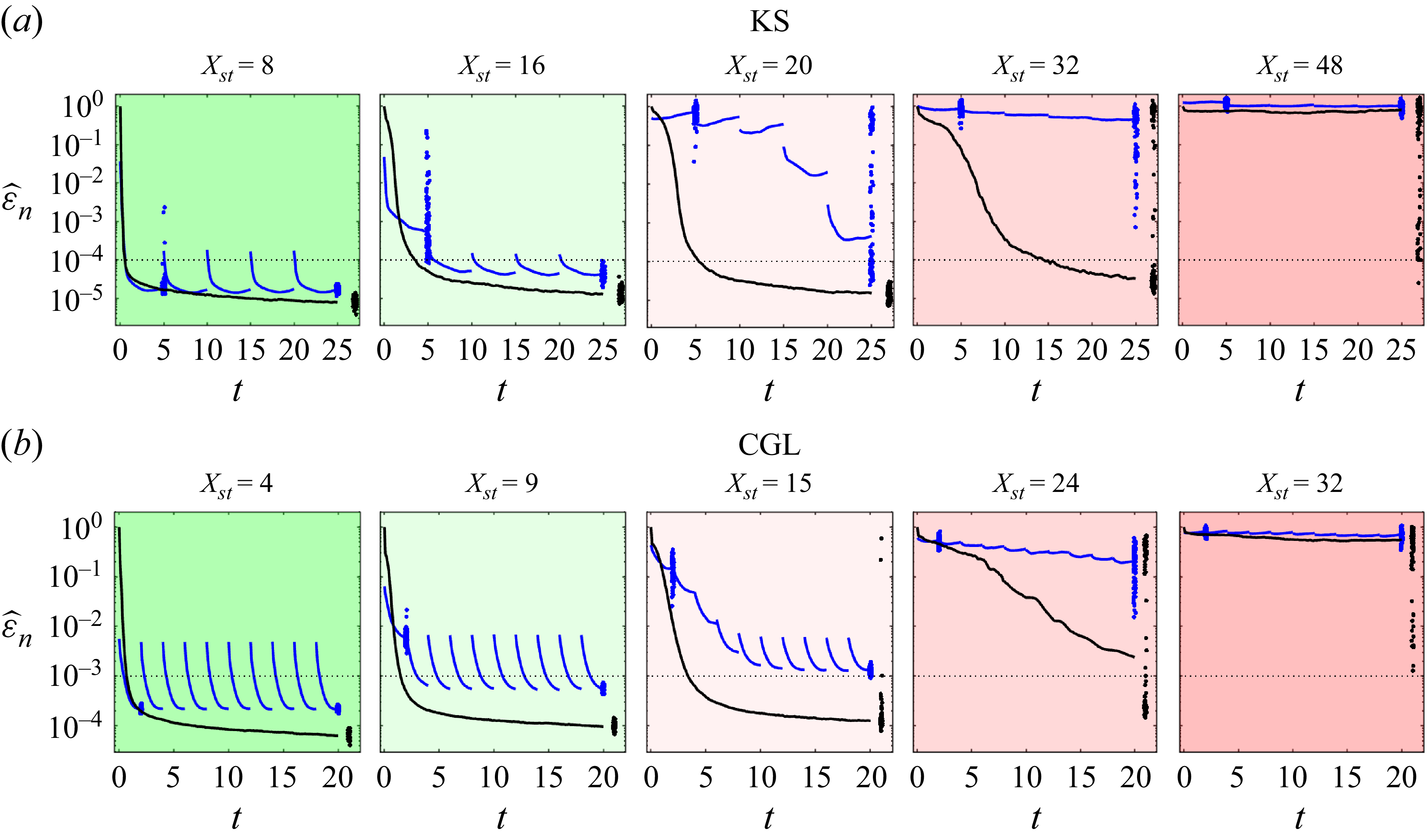
Figure 2 presents the median error
 $\hat {\varepsilon }_n(t)$
over 100 independent runs for full field reconstruction of the KS and CGL systems using 4D-Var (blue) and EnKF (black). The observations are at the
 $X_{\textit{st}}$
indicated, with green (red) shading representing observations denser (sparser) than the DS critical resolution. Other observation parameters are
 $(T_{\textit{st}},\sigma ) = (2,10^{-4}s_u)$
for the KS system and
 $(T_{\textit{st}},\sigma ) = (5,10^{-3}s_u)$
for the CGL system. These
 $(T_{\textit{st}},\sigma )$
values mean that the sampling rate is high with respect to the Lyapunov time scale
 $\varLambda _{\textit{max}}^{-1}$
, and the noise level (indicated by the dotted lines) is low with respect to the signal strength. Scattered dots represent
 $\varepsilon _n$
from individual runs: for 4D-Var, errors are shown after the first and last sequences, while for EnKF, they are shown at the end of the assimilation time. The EnKF parameters for the KS system are
 $N_{\textit{ens}}= (512,512,2048,2048,2048)$
and
 $\gamma =(1,1,1,1.01,1.01)$
, and for the CGL system they are
 $N_{\textit{ens}} = (1024,1024,4096,4096,4096)$
and
 $\gamma =(1,1,1,1.02,1.02)$
. The 4D-Var parameter
 $N_{\textit{iter}}$
exceeds 100 in all panels, except the first column, and further increasing
 $N_{\textit{iter}}$
does not significantly improve the reconstruction quality.
The evolution of
 $\widehat {\varepsilon }_n$
in full field reconstruction of the (a) KS and (b) CGL systems using 4D-Var (blue) and EnKF (black). The observations are at
 $X_{\textit{st}}$
values indicated above the plots, and at (a)
 $(T_{\textit{st}},\sigma ) = (2,10^{-4}s_u)$
and (b)
 $(T_{\textit{st}},\sigma ) = (5,10^{-3}s_u)$
. The scattered dots are
 $\varepsilon _n$
for the individual runs after the first and last sequences for 4D-Var, and at the end of assimilation time for EnKF.

The first column of figure 2 shows the median estimation errors when observations are more than twice the DS critical resolution. Both EnKF and 4D-Var errors rapidly converge to values below the observation errors, demonstrating an accurate reconstruction of the full field within the observation error limit. The 4D-Var errors converge within the first sequence, and during this period, their median values are lower than those of EnKF. This advantage arises because 4D-Var utilises all observations within the DAW of a sequence, whereas EnKF processes observations sequentially, using less information per update. After the first sequence, the subsequent 4D-Var sequences show no further reduction in the median error, but a clear decrease in error scatter is observed, particularly for the KS system. This indicates that some cases initially stuck in local minima during the first sequence eventually converged to the ground truth. Here, EnKF continuously updates the matrix
 $\mathcal{B}_{\!j}^f$
to refine the estimated field, and its errors eventually converge to slightly lower median values than those of 4D-Var, although the difference is practically negligible.
The second column of figure 2 shows the median estimation errors when observations are slightly denser than the DS critical resolution. While the errors still converge to values below the observation errors, the rates of convergence are slower compared to the first column. This is because relatively less information is now available within the same time frame as compared to the first column. Notably, the 4D-Var errors at the end of the first sequence are significantly higher than the EnKF errors at that time. In fact, the median 4D-Var errors drop below the observation errors only from the second sequence onwards. This delay in 4D-Var convergence may stem from two factors: insufficient information within the first sequence to ensure convergence to the ground truth, or the 4D-Var estimation getting stuck in a local minimum. Because EnKF exhibits rapid convergence, indicating sufficient information within the first sequence, the latter reason appears more likely. If the initial guess is too far from the optimal solution, then there is a chance that 4D-Var may converge to a local minimum (see Appendix C for more details). This limitation is inherent to 4D-Var (Pires, Vautard & Talagrand Reference Pires, Vautard and Talagrand1996; Hoteit Reference Hoteit2008) and has also been reported by Wang & Zaki (Reference Wang and Zaki2025).
The third column of figure 2 shows the median estimation errors when observations are slightly sparser than the DS critical resolution. In most cases, both EnKF and 4D-Var errors still converge to values below the observation error, demonstrating that DA methods can accurately reconstruct the full field even with observations sparser than the DS critical resolution. However, the convergence rates of the two DA methods now differ significantly. The 4D-Var errors remain high after the first sequence, indicating poor reconstruction quality, which may lead to the conclusion that 4D-Var struggles when observations fall below the critical resolution (Page Reference Page2025). In contrast, EnKF maintains performance similar to that in the first two columns, though with slightly slower convergence. Notably, EnKF in the third column and beyond uses four times more ensemble members than in the first two columns. This is because a larger search space is required by the ensemble members to converge to the ground truth from the sparse observations (Gottwald & Majda Reference Gottwald and Majda2013). Two EnKF runs in the CGL case fail to converge to the ground truth, an issue further explored in § 3.3. From the third column onwards, the 4D-Var and EnKF errors from different runs are scattered across different orders of magnitude. This happens because of 4D-Var runs getting stuck in a local minimum, and because of ensemble collapse in EnKF (see Appendix C for more details).
The fourth and fifth columns of figure 2 show the median estimation errors when observations are nearly two and three times sparser than the DS critical resolution, respectively. For many cases, the EnKF errors still converge to values below the observation errors, demonstrating that EnKF can accurately reconstruct the full field even from highly sparse observations. However, EnKF now requires inflation, because the limited information available at each update increases the risk of ensemble members diverging from the attractor (Gottwald & Majda Reference Gottwald and Majda2013). In contrast, the 4D-Var errors in these cases do not converge to values below the observation errors, but exhibit a continuous decrease over time. We show in § 3.3 that both 4D-Var and EnKF may eventually converge to the ground truth across all cases even with such extreme sparsity in observations.
The ground truth (top panel), observed (middle column) at
 $X_{\textit{st}}=$
16, 32 and 48, and the corresponding predicted fields from 4D-Var (first column) and EnKF (last column) for the KS system.

The ground truth (top panel), observed (middle column) at
 $X_{\textit{st}}=$
9, 24 and 32, and the corresponding predicted fields from 4D-Var (first column) and EnKF (last column) for the CGL system.

The evolution of
 $\widehat {\varepsilon }_n$
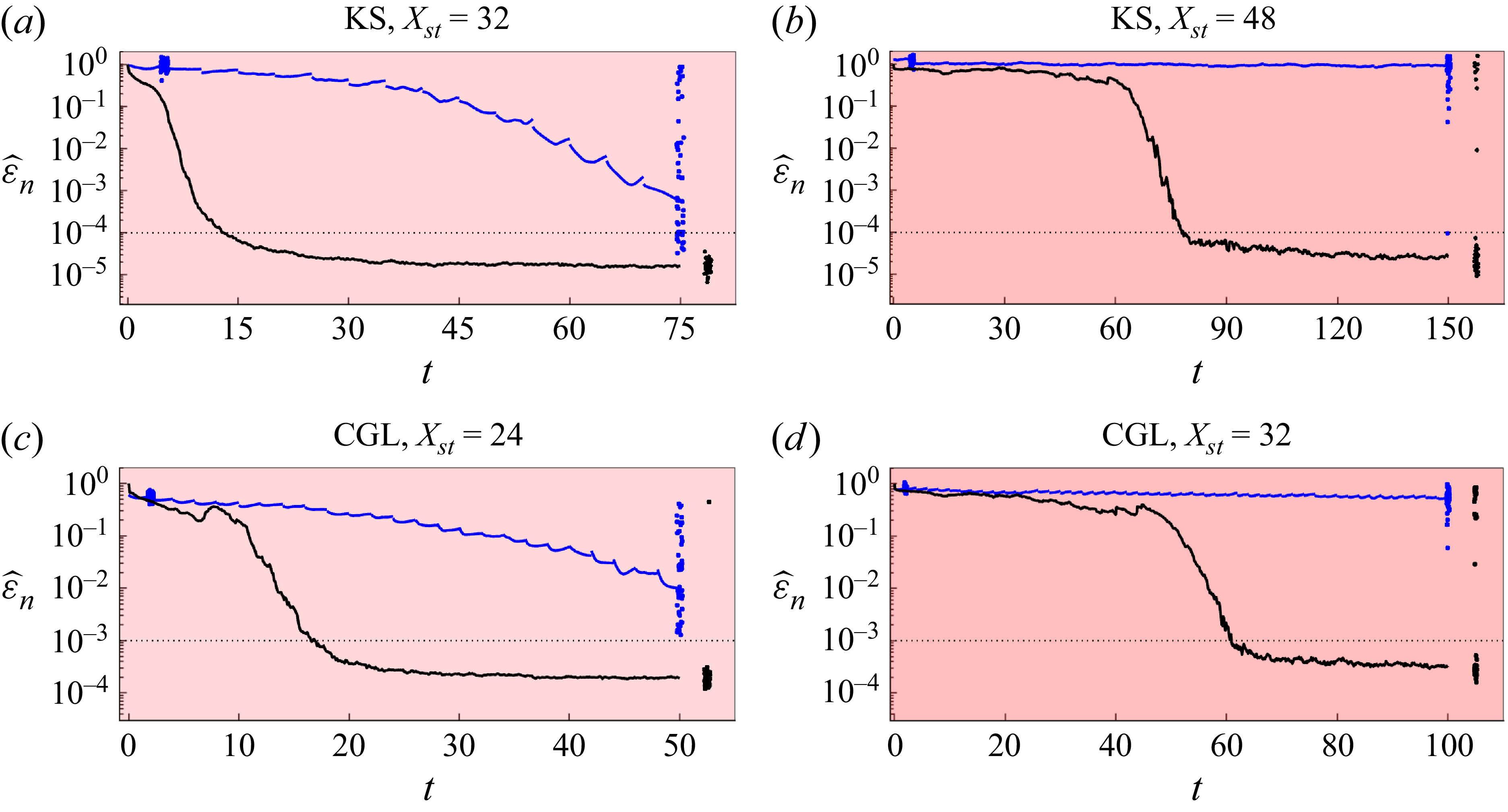
in full field reconstruction over extended assimilation time using 4D-Var (blue) and EnKF (black) for the (a,b) KS and (c,d) CGL systems under extreme observation sparsity. Parameter
 $X_{\textit{st}}$
is given above the plots, while
 $(T_{\textit{st}},\sigma )$
and other details are the same as in figure 2.

Figure 3 presents the ground truth and predicted flow fields (from one run of 4D-Var and EnKF) for the KS system with observations at
 $X_{\textit{st}}= 16$
(second row),
 $X_{\textit{st}}= 32$
(third row) and
 $X_{\textit{st}}= 48$
(fourth row). Similarly, figure 4 shows the corresponding results for the CGL system, with observations at
 $X_{\textit{st}}= 9$
(second row),
 $X_{\textit{st}}= 24$
(third row) and
 $X_{\textit{st}}= 32$
(fourth row). These results confirm that both DA methods can accurately reconstruct the full fields, even when observations are sparser than the DS critical resolution. The final rows in both figures visually highlight the strength of EnKF in rapidly converging to the ground truth, even under extreme observation sparsity.
3.3. Long-term assimilation of cases with extreme observation sparsity
Figure 5 presents the median estimation error
 $\widehat {\varepsilon }_n$
over 50 independent runs, for the highly sparse cases shown in the last two columns of figure 2, now extended over a longer assimilation time. For both systems, the 4D-Var parameter is set to
 $N_{\textit{iter}}=50$
, while the EnKF parameters remain the same as in figure 2. Here, we employ a restart strategy for EnKF when its predictions diverge from the ground truth even at the observation points. If the RMSE between EnKF predictions at observation points and the observations exceeds a threshold
 $3\sigma$
, then the ensemble members are reinitialised and EnKF is resumed.
The results in figures 5(a,c) show that EnKF errors for nearly all runs (except for one in figure 5 c) have converged to values below the observation errors. For 4D-Var, several runs have also converged to values below the observation errors, but longer assimilation time appears necessary for full convergence. Figures 5(b,d) show qualitatively similar results to figures 5(a,c). However, the need for longer assimilation time is evident before all runs can converge to the ground truth. These results demonstrate that both 4D-Var and EnKF can converge to the ground truth even under extreme observation sparsity. However, the likelihood of achieving convergence within a given assimilation time decreases significantly as sparsity increases. This implies that much longer assimilation times may be necessary for accurate full field reconstruction as observations become sparser. Comparing the two methods, 4D-Var generally requires significantly more assimilation time than EnKF. However, unlike EnKF, 4D-Var does not rely on ad hoc stabilisation techniques.
3.4. Estimation errors at different temporal sparsity levels
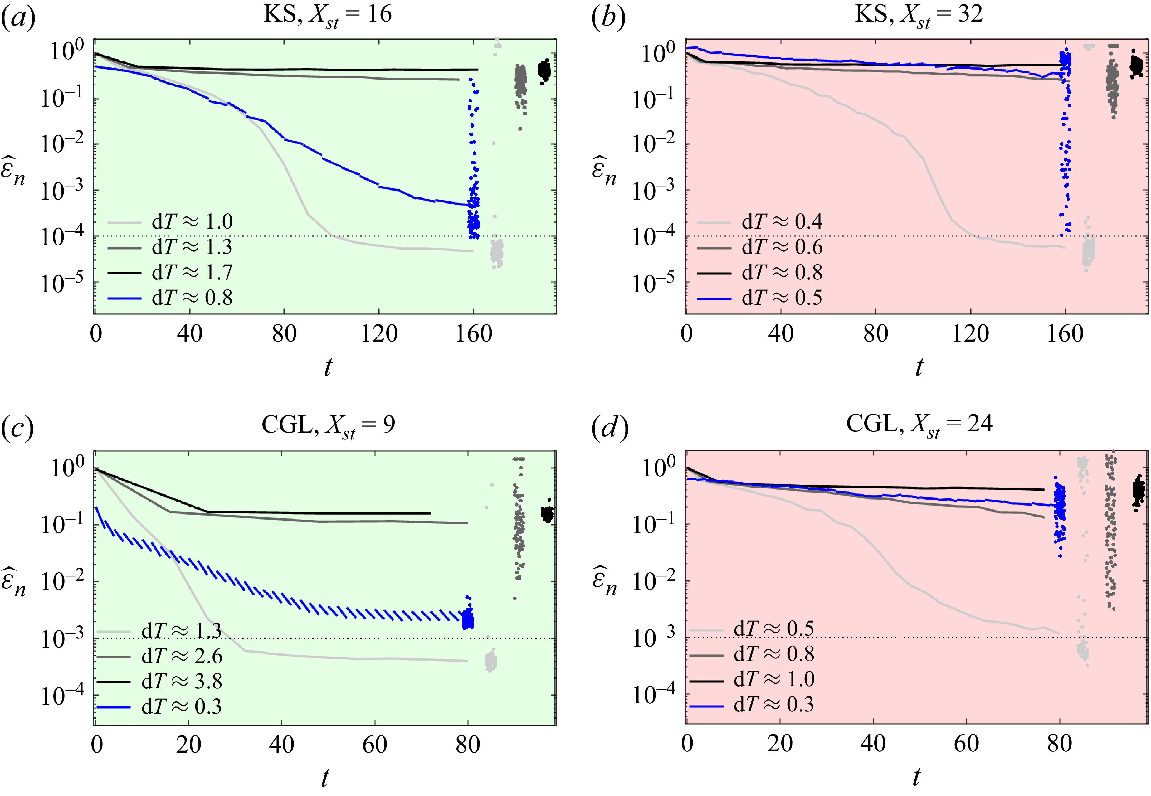
We now examine the ability of the DA methods to reconstruct the full field when observations are also sparse in time. Figure 6 presents the median estimation error
 $\hat {\varepsilon }_n$
over 100 runs for the KS and CGL systems. The parameter
 $X_{\textit{st}}$
is specified at the top of each plot, and
 $T_{\textit{st}}\,{\rm d}t$
is of
 $O(\varLambda _{\textit{max}}^{-1})$
. Therefore, we use the parameter
 ${\rm d}T = T_{\textit{st}}\,{\rm d}t/\varLambda _{\textit{max}}^{-1}$
to indicate the temporal sparsity. For 4D-Var (blue lines), the DAW for each sequence is equal to
 ${\rm d}T\,\varLambda _{\textit{max}}^{-1}$
, and
 $N_{\textit{iter}}=50$
. For EnKF (grey and black lines), the parameters remain the same as in figure 2. The observation noise and other details are the same as in figure 2.
The evolution of
 $\widehat {\varepsilon }_n$
in full field reconstruction using 4D-Var (blue) and EnKF (grey and black) for the (a,b) KS and (c,d) CGL systems from spatiotemporally sparse observations. The parameter
 $X_{\textit{st}}$
is given above the plots, and
 ${\rm d}T = T_{\textit{st}}\,{\rm d}t/\varLambda _{\textit{max}}^{-1}$
is indicated in the legends. Other details are the same as in figure 2.

The results in figure 6 demonstrate that the DA methods can accurately reconstruct flow fields under temporal sparsity of the order of
 $\varLambda _{\textit{max}}^{-1}$
. As expected, the level of temporal sparsity that allows accurate reconstruction decreases as spatial sparsity increases; this is also observed in Wang & Zaki (Reference Wang and Zaki2021). For 4D-Var, the DAW for each sequence is limited to approximately
 $\varLambda _{\textit{max}}^{-1}$
, meaning that 4D-Var cannot handle
 ${\rm d}T$
values exceeding the DAW. For EnKF, the corrections at each observation time are linear, which can restrict its ability to manage larger time steps. For the systems analysed here, EnKF generally performs better than 4D-Var in handling temporal sparsity. Fossella et al. (Reference Fossella, Biferale, Carrassi, Cencini and Gupta2026), for estimation of a shell model of turbulence, also found that EnKF can handle temporal sampling steps exceeding the DAW required for 4D-Var. However, it is uncertain whether this advantage of EnKF will be held for systems with stronger nonlinearity. It is also worth noting that our results do not indicate a fixed cut-off for
 ${\rm d}T$
beyond which reconstruction becomes impossible, as observed in Meldi (Reference Meldi2018). This discrepancy may arise because the systems studied here lack advection and the separation between boundary and sensor locations.
4. Application of EnKF to turbulent two-dimensional Kolmogorov flow
In this section, we examine turbulent two-dimensional Kolmogorov flow for which 4D-Var and ML are recently applied in Page (Reference Page2025) for full field reconstruction from spatiotemporally sparse observations, also called super-resolution. This system is expressed as
 \begin{equation} \partial _t \omega + u_x\, \partial _{x}\omega + u_y\,\partial _{\!y}\omega = \frac {1}{\textit{Re}}\big (\partial _x^2 \omega + \partial _y^2 \omega \big ) - \alpha \omega - n_{\!f} \cos (n_{\!f} y), \end{equation}
where
 $\omega$
is the out-of-plane vorticity,
 $(u_x,u_y)$
are the velocity components in the
 $(x,y)$
directions,
 $\boldsymbol{Re}=1000$
is the Reynolds number,
 $\alpha =0.1$
is the drag factor that prevents accumulation of energy in large scales, and
 $n_{\!f}=4$
is the wavenumber at which monochromatic Kolmogorov forcing is applied (note that the forcing appears as
 $\sin (n_{\!f} y)$
in the
 $x$
-momentum equation). The system is periodic in both directions with the domain size
 $2\pi \times 2\pi$
, and the non-dimensional time is such that
 $t=1$
is one eddy turnover time. These parameters are the same as in the recent studies of Page (Reference Page2025) and Inubushi & Caulfield (Reference Inubushi and Caulfield2025). The ground truth is obtained using JAX-CFD code (Kochkov et al. Reference Kochkov, Smith, Alieva, Wang, Brenner and Hoyer2021) with
 $256\times 256$
grid points – compared to
 $512\times 512$
in Page (Reference Page2025), and
 $128 \times 128$
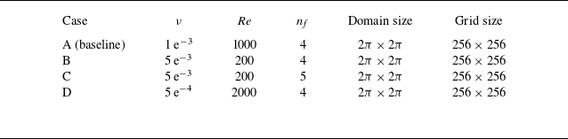
in Inubushi & Caulfield (Reference Inubushi and Caulfield2025). The JAX-CFD code at the same resolution is also used for flow reconstruction using EnKF, i.e. the perfect model is known. In addition to this baseline case (called case A), we analyse three more cases at varying
 $\boldsymbol{Re}$
and
 $n_{\!f}$
as summarised in table 1. Observations are the downsampled velocity components in space, where downsampling by
 $X_{\textit{st}}$
is performed in both spatial directions.
The physical and numerical parameters of the four Kolmogorov flow cases.

For case A, Page (Reference Page2025) finds that 4D-Var is unable to accurately reconstruct the flow field when observations are sparser than the DS critical resolution, while Inubushi & Caulfield (Reference Inubushi and Caulfield2025) link the DS critical resolution to the forced wavenumber
 $n_{\!f}$
. Here, we will first obtain the DS critical resolution for the four Kolmogorov flow cases, and then perform EnKF at varying sparsity levels. We do not perform 4D-Var because it is computationally expensive, and requires formulating an adjoint solver. Instead, we use the 4D-Var results from Page (Reference Page2025) for comparison, which we find sufficient to draw conclusions.
4.1. Critical resolution from DS for chaos synchronisation
Figures 7(a i–d i) present the mean estimation error
 $\overline {\varepsilon }$
over 10 runs, for full field reconstruction of the Kolmogorov flow cases using DS with observations at
 $X_{\textit{st}} = 15$
–20. We note that
 $\overline {\varepsilon }$
converges to
 $O(10^{-4})$
instead of the machine precision. This is because the simulations are performed for the
 $\omega$
field, while errors are calculated for the velocity fields. If DS were performed with
 $\omega$
measurements in the Fourier space, as done in Inubushi & Caulfield (Reference Inubushi and Caulfield2025), then the errors would converge to machine error, and fewer Fourier modes as compared to spatial observation points would be required for chaos synchronisation. However, such measurements are not practical (Page Reference Page2025), thus we perform DS with spatially sparse measurements of the
 $(u_x,u_y)$
fields.
(a i–d i) The evolution of
 $\overline {\varepsilon }_n$
in full field reconstruction of the Kolmogorov flow cases using DS. (a ii–d ii) Samples of the
 $u_x$
fields at a time instant (see figure 9 for colour bar). (a iii–d iii) The time-averaged energy spectra. These results show that as
 $\boldsymbol{Re}$
and
 $n_{\!f}$
increase, the DS critical resolution also increases.

The results in figures 7(a i–d i) show that the DS critical resolution is
 $X_{\textit{st}}=18$
for case A,
 $X_{\textit{st}}=19$
for case B,
 $X_{\textit{st}}=17$
for case C, and
 $X_{\textit{st}}=16$
for case D. Comparisons between different cases show that higher resolution observations are required by the DS method as either
 $\boldsymbol{Re}$
or
 $n_{\!f}$
increases. This could be because the increase in
 $\boldsymbol{Re}$
or forcing at higher
 $n_{\!f}$
increases the contribution from higher wavenumbers (see figures 7
a iii–d iii). Notably, the effect of increasing
 $n_{\!f}$
from 4 to 5 (case B to case C) is nearly the same as increasing
 $\boldsymbol{Re}$
by an order of magnitude (case B to case D). This agrees well with Inubushi & Caulfield (Reference Inubushi and Caulfield2025), who relate the DS critical resolution with
 $n_{\!f}$
.
Figures 7(a ii–d ii) show the samples of fully resolved
 $u_x$
fields, and figures 7(a iii–d iii) show the time-averaged energy spectrum
 $E(k)$
against the wavenumber
 $k$
. The time-averaging is performed from
 $t=0$
to
 $t=5$
. These results show that
 $E(k)$
decays slower in higher
 $\boldsymbol{Re}$
flows, thus increasing the contribution of high wavenumbers with increasing
 $\boldsymbol{Re}$
. For higher
 $n_{\!f}$
flows, however, the decay rate of
 $E(k)$
appears to slightly increase. Nevertheless, forcing at a higher
 $n_{\!f}$
significantly increases the contribution of higher wavenumbers close to
 $n_{\!f}$
.
4.2. Estimation errors at different spatial sparsity levels for case A
We perform EnKF for reconstructing the full field of case A with observations available at
 $X_{\textit{st}}=8$
, 16, 32 and 64. Note that
 $X_{\textit{st}}=M/2$
in Page (Reference Page2025), meaning the
 $X_{\textit{st}}=8$
and 16 here correspond to
 $M=16$
and 32 in Page (Reference Page2025). Other observation parameters are
 $(T_{\textit{st}},\sigma ) = (8,0)$
, which align with the
 $M=16$
case in Page (Reference Page2025). Although the observations are noise-free, the EnKF method still requires adding noise to the observations. Therefore, for the EnKF results presented here, the effective observation noise is set as
 $\sigma = 0.020$
for the
 $X_{\textit{st}}=8$
case, and
 $\sigma =0.005$
for the other three cases. The initial ensemble comprises the random realisations of the system, i.e. they are statistically uncorrelated from each other as well as with the ground truth (see Appendix A for further details on EnKF).
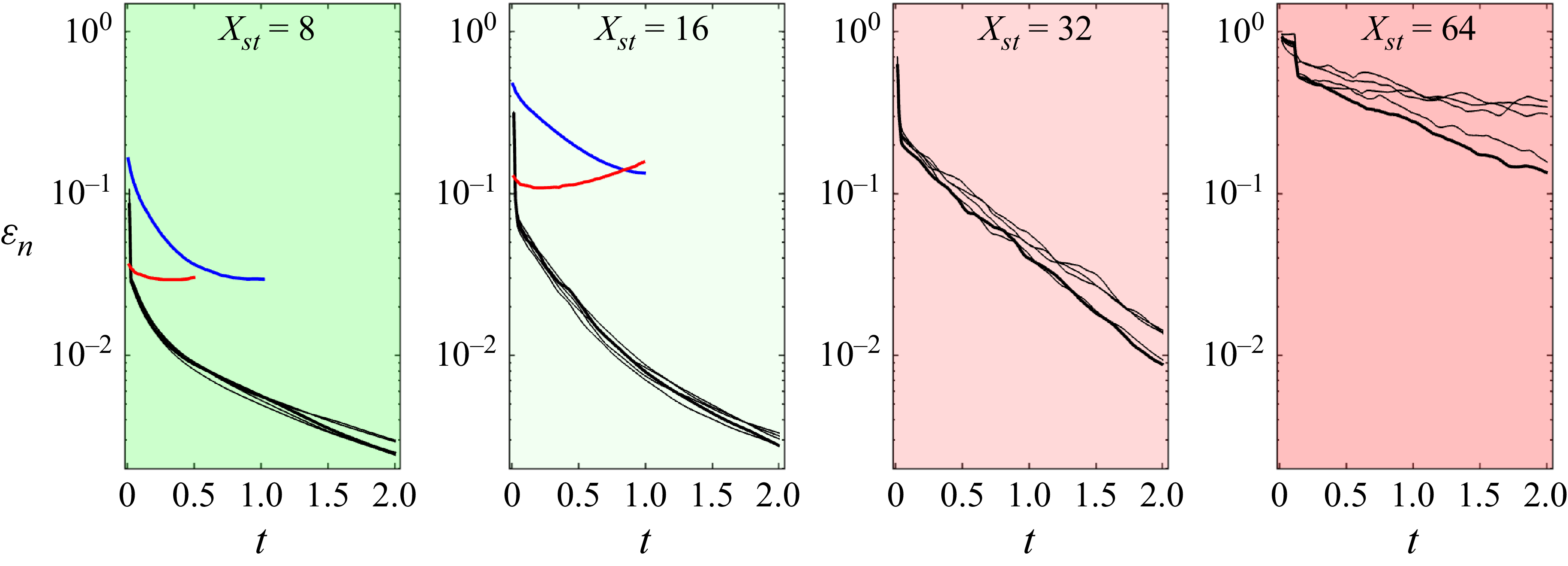
The evolution of
 $\varepsilon _n$
in full field estimation for case A of the Kolmogorov flow when observations are at
 $X_{\textit{st}}$
as indicated at the top of the plots, and at
 $(T_{\textit{st}},\sigma ) = (8,0)$
. The five black curves are the EnKF errors for five independent runs, while the blue and red lines are the averaged 4D-Var and ML errors, respectively, from Page (Reference Page2025).

Figure 8 shows
 $\varepsilon _n$
for five independent runs where EnKF with
 $N_{\textit{ens}}=4096$
is used for full field reconstruction (black lines), alongside the averaged 4D-Var errors (blue lines) and ML errors (red lines) from Page (Reference Page2025). The results demonstrate that estimation errors decrease in all cases and for all runs, confirming that EnKF can successfully reconstruct the full field even under extreme observation sparsity. However, the rate of error convergence slows down and becomes more uncertain as sparsity increases, leading to greater dispersion among the five runs at higher
 $X_{\textit{st}}$
values. Additionally, the difference between EnKF and 4D-Var errors is more pronounced for the
 $X_{\textit{st}} = 16$
case than for the
 $X_{\textit{st}}=8$
case. This suggests an increasing tendency for 4D-Var to become trapped in local minima as sparsity grows. These findings, observed for the KS and CGL systems in § 3, now confirm their applicability to a two-dimensional turbulent flow. We also plot the errors from the ML method used in Page (Reference Page2025), which is based on the ResNet architecture. The ML reconstruction is superior to that from 4D-Var, particularly at the beginning of the assimilation window. Our results show that EnKF outperforms the ML reconstruction from the second assimilation step itself. Although these results cannot be used to conclude that EnKF (or DA) can outperform ML in general, they highlight the need for benchmarking ML results against conventional DA.
The ground truth (top panel), observed (second row), and EnKF predicted (third row)
 $u_x$
fields at
 $t=2$
for the Kolmogorov flow when
 $X_{\textit{st}}=$
8, 16, 32 and 64 (first to fourth columns). The last row is the energy spectra of the ground truth (red), the predicted fields (black) and the error fields (dash-dotted black).

Figure 9 presents the ground truth (top panel), observed (second row) and predicted (third row) flow fields from EnKF at
 $t=2$
, with observations at
 $X_{\textit{st}}= 8$
, 16, 32 and 64 (from the first to fourth columns). The chosen run corresponds to the thick black line in figure 8, which demonstrates good performance across all cases. These results visually confirm that EnKF can successfully reconstruct the full field from highly sparse observations. The bottom row displays the instantaneous energy spectrum of the ground truth (red lines with markers), EnKF predictions (black lines), and the error (dash-dotted black lines). The two vertical dashed lines correspond to
 $n_{\!f}$
and the wavenumber
 $k_m$
up to which information can be obtained from sparse observations as per the Nyquist criterion (note that the wavenumber modes up to
 $k_m$
obtained from spatially sparse data will have significant aliasing errors). The dotted line indicates
 $k^{-4}$
power-law scaling. These results show that except for the
 $X_{\textit{st}}=64$
case, EnKF accurately reconstructs the flow across all wavenumbes by the assimilation time
 $t=2$
.
The ground truth (top panel), observed (second row), the EnKF predicted (third row)
 $u_x$
fields, and the energy spectra as in figure 9 (bottom row) at
 $t=T$
,
 $3T$
and
 $5T$
when
 $X_{\textit{st}}= 64$
.

Figure 10 shows the EnKF predictions for the
 $X_{\textit{st}}=64$
case, using the same run as in figure 9, for an extended assimilation time from
 $t=0$
to
 $t=5$
. The first row shows the ground truth, the second row shows the observations, the third row shows the predicted fields, and the fourth row shows the spectra. The columns correspond to times
 $t=1$
,
 $3$
and
 $5$
, respectively. These results confirm that EnKF accurately reconstructs the full field even under extreme observation sparsity, provided that it is allowed to run for several eddy turnover times. Notably, the observations in this case are 14 times sparser than the DS critical resolution, and cover only
 $0.024\,\%$
of the computational grid points. Furthermore, the observations do not include any wavenumbers even in the inertial range.
4.3. Application of EnKF to Kolmogorov flows at varying
 $\boldsymbol{Re}$
and
$n_{\!f}$


Figure 11 presents EnKF results for full field reconstruction of cases B–D, which represent the Kolmogorov flows at varying
 $\boldsymbol{Re}$
and
 $n_{\!f}$
. We keep the spatial sparsity of observations at
 $X_{\textit{st}}=64$
, i.e.
 $4\times 4$
observations, and temporal sparsity at
 $T_{\textit{st}}=8$
for all cases. The top row shows the evolution of
 $\varepsilon _n$
in full field estimation of these cases. The second to fourth rows show
 $u_x$
fields for the ground truth, observations and EnKF predictions at
 $t=5$
. The bottom row shows the corresponding
 $E(k)$
of the ground truth (red lines with markers), EnKF predictions (black lines) and error (dash-dotted lines).
The evolution of
 $\varepsilon _n$
(top row) in full field estimation of cases B–D of the Kolmogorov flow when observations are at
 $(X_{\textit{st}},T_{\textit{st}},\sigma ) = (64,8,0)$
. The ground truth (second row), observed (third row), EnKF predicted (fourth row)
 $u_x$
fields, and the energy spectra as in figure 9 (bottom row) at
 $t=5$
.

These results show that EnKF is able to perform full field reconstruction from a
 $4\times 4$
observation grid for the Kolmogorov flows at varying
 $\boldsymbol{Re}$
and
 $n_{\!f}$
. We know from the DS method in § 4.1 that reconstruction becomes increasingly difficult with increasing
 $\boldsymbol{Re}$
and
 $n_{\!f}$
, thus requiring higher resolution observations for cases with higher
 $\boldsymbol{Re}$
and
 $n_{\!f}$
. The EnKF method can reconstruct all these cases from a
 $4\times 4$
observation grid, but uses a larger
 $N_{\textit{ens}}$
for cases with higher
 $\boldsymbol{Re}$
and
 $n_{\!f}$
. The case with lowest
 $\boldsymbol{Re}$
and
 $n_{\!f}=4$
, i.e. case B, needs approximately
 $N_{\textit{ens}}=2048$
for successful reconstruction. Keeping
 $n_{\!f}=4$
, the increases in
 $\boldsymbol{Re}$
to 1000 and 2000 in cases A and D require
 $N_{\textit{ens}}=4096$
and 16 384, respectively. While keeping
 $\boldsymbol{Re}=200$
, the increase in
 $n_{\!f}$
to 5 in case C requires
 $N_{\textit{ens}}=8192$
. (We change
 $N_{\textit{ens}}$
in powers of 2.) Note that the rate of error reduction slows down with increasing flow complexity. Requirement of larger
 $N_{\textit{ens}}$
with increasing flow complexity highlights a drawback of EnKF. With our current computational resources, limited to 64 GB memory, we cannot deal with more complex cases unless we employ ad hoc measures such as localisation to rectify erroneous long-range correlations.
5. Discussion
In this section, we discuss the implications of our results for prediction and estimation of turbulent flows from sparse observations.
5.1. How sparse in space can the observations be for full field reconstruction?
Sparse observations at a single time instant can correspond to multiple system states, making it an ill-posed problem to reconstruct the full field from such observation alone. However, if sparse observations are gathered over a sufficiently long period and at a high enough sampling rate, then these observations may correspond to a unique system state. Takens’ embedding theorem (Takens Reference Takens1981) suggests that observations collected even at a single point would suffice – provided that the boundary conditions and governing equations are known – to uniquely determine the system state. A relatively conservative notion of determining nodes was introduced by Foias & Temam (Reference Foias and Temam1984), which states that the minimum number of observation points required (for a spatially periodic system) is equal to the highest spatial derivative in the system. This implies that the number of observations is 4 for the KS system (
 $X_{\textit{st}}=128$
), 2 for the CGL system (
 $X_{\textit{st}}=256$
), and
 $2\times 2$
for the Kolmogorov flow (
 $X_{\textit{st}}=128$
).
The results in figures 5, 10 and 11 demonstrate that DA methods can achieve reconstruction with observation sparsity levels close to the determining nodes limit, particularly for the KS system (10 observation points) and the Kolmogorov flow (
 $4\times 4$
observation points irrespective of the flow complexity, which increases with increasing
 $\boldsymbol{Re}$
and
 $n_{\!f}$
). This suggests that EnKF and 4D-Var are capable of accurately reconstructing the full field of turbulent systems from observations at near-theoretical sparsity levels. (The determining node limit does not restrict observations to be equispaced, as is the case here, and is valid only in the
 $t\to \infty$
limit.) However, it is important to note that the systems analysed here, including the turbulent two-dimensional Kolmogorov flow, have weaker small-scale intermittency compared to high Reynolds number three-dimensional turbulence. Fossella et al. (Reference Fossella, Biferale, Carrassi, Cencini and Gupta2026) applied EnKF, nudging and 4D-Var to reconstruct a shell model of turbulence from intermediate scale observations. The shell model, despite having only a few degrees of freedom, mimics the multi-scale intermittent nature of high-
 $\boldsymbol{Re}$
three-dimensional turbulence (Biferale Reference Biferale2003). The results in Fossella et al. (Reference Fossella, Biferale, Carrassi, Cencini and Gupta2026) show that reconstructing smaller intermittent scales is more challenging than reconstructing the larger scales.
5.2. How sparse in time can the observations be for full field reconstruction?
Chaotic systems have a finite memory, beyond which they effectively lose information about their initial state, because even infinitesimal errors grow exponentially at a rate determined by
 $\varLambda _{\textit{max}}$
. As a result, if observations are too sparse in time, then they cannot be consistently linked to a unique system state, making the full field reconstruction an ill-posed problem. However, it is worth noting that large-scale features may still be predicted without reconstructing the smaller scales (Leith & Kraichnan Reference Leith and Kraichnan1972). Our findings show that a higher sampling rate is necessary when spatial observations are sparser, as also noted in Wang & Zaki (Reference Wang and Zaki2021), and that EnKF outperforms 4D-Var at lower sampling rates. The advantage of EnKF over 4D-Var at lower temporal sampling rates may also be inferred from the results in Fossella et al. (Reference Fossella, Biferale, Carrassi, Cencini and Gupta2026). Nevertheless, these conclusions may require further validation for flows with stronger nonlinearity and those dominated by advection (Meldi Reference Meldi2018).
5.3. Choosing 4D-Var or EnKF
For a linear system with Gaussian errors, theoretically, 4D-Var and Kalman filter should give identical results at the end of the DAW. For nonlinear systems, both 4D-Var and EnKF cannot fully account for the system nonlinearities. In 4D-Var, the minimisation of the cost function requires a tangent linear hypothesis. In EnKF, the updates are linearly proportional to the forecast errors. Therefore, the effectiveness of both methods is situation dependent. Based on the results presented here, EnKF appears to have certain advantages, including the ability to reconstruct within a smaller assimilation time and at lower sampling rate. The EnKF method also has the advantage of not requiring an adjoint model, making its implementation easier. However, EnKF requires higher memory and relies on ad hoc stabilisation techniques, such as inflation, and potentially localisation for larger systems. In contrast, 4D-Var does not require such ad hoc measures, making it preferable for systems where long time series data and ample computational resources are available. Additionally, 4D-Var may converge slightly faster by incorporating background information (Bauweraerts & Meyers Reference Bauweraerts and Meyers2021) or simulated annealing (Hoteit Reference Hoteit2008), but they significantly increase the computational cost.
Another advantage of 4D-Var is its proven track record within the turbulence community. For example, Papadakis & Mémin (Reference Papadakis and Mémin2008) and Heitz, Mémin & Schnörr (Reference Heitz, Mémin and Schnörr2010) demonstrated its use for state estimation from sequences of noisy measurements, while Gronskis, Heitz & Mémin (Reference Gronskis, Heitz and Mémin2013) and Hayase (Reference Hayase2015) applied it for obtaining the initial condition, showcasing its suitability for experimental settings. Furthermore, for cases where the governing equations are not precisely known, dynamic error models (Chandramouli et al. Reference Chandramouli, Memin and Heitz2020) and weak formulation frameworks (He et al. Reference He, Zeng, Wang, Wen and Liu2024) have been developed for 4D-Var. The method has also been coupled with optimal sensor placement strategies (Mons & Marquet Reference Mons and Marquet2021; Mons, Vervynck & Marquet Reference Mons, Vervynck and Marquet2024). By comparison, the applications of EnKF for full field reconstruction are fewer (Colburn et al. Reference Colburn, Cessna and Bewley2011; Suzuki Reference Suzuki2012; Kato et al. Reference Kato, Yoshizawa, Ueno and Obayashi2015; Suzuki & Hasegawa Reference Suzuki and Hasegawa2017), though recent progress has been made with regularised EnKF (Zhang, Michelén-Ströfer & Xiao Reference Zhang, Michelén-Ströfer and Xiao2020) and parallel EnKF approaches (Zhang, Zhang & He Reference Zhang, Zhang and He2024). Our results show that both EnKF and 4D-Var can reconstruct turbulent flows with much sparser resolution than required by DS for chaos synchronisation, while their implementations have strengths and trade-offs. Further such comparisons are warranted for systems with model errors, which require weak-formulation 4D-Var, a nonlinear observation operator, and non-Gaussian observation errors.
5.4. Choosing DA or ML
As an alternative to DA, several model-free ML methods have been recently developed for full field reconstruction of turbulent flows. The key advantages of ML methods are that they do not require knowledge of the governing equations, and once trained, they are computationally much faster than DA. Even the turbulent two-dimensional Kolmogorov flow studied here is simulated using an ML-trained code (Kochkov et al. Reference Kochkov, Smith, Alieva, Wang, Brenner and Hoyer2021). Numerous ML frameworks demonstrate the ability to reconstruct full fields from highly sparse observations (Fukami et al. Reference Fukami, Fukagata and Taira2021; Li et al. Reference Li, Han, Zhang, Fu, Li, Qin, Dong, Sun, Deng and Yang2024b
). However, the lack of systematic benchmarking means that these approaches are yet to be methodically compared. The results in Li et al. (Reference Li, Han, Zhang, Fu, Li, Qin, Dong, Sun, Deng and Yang2024b
) for the KS system appear to operate at sparsity levels similar to those in the current work. However, to our knowledge, applications of ML for super-resolution of the Kolmogorov flow (Fukami et al. Reference Fukami, Fukagata and Taira2021; Fukami & Taira Reference Fukami and Taira2024; Page Reference Page2025) use denser observations than the
 $4\times 4$
observations used here. Comparisons between ML and DA methods, conducted over multiple independent runs and with perturbed system parameters, could yield intriguing insights.
6. Conclusion
In this paper, we apply EnKF and 4D-Var for full field reconstruction from spatiotemporally sparse observations of three systems: (i) KS system exhibiting phase turbulence, (ii) CGL system exhibiting defect chaos, and (iii) turbulent two-dimensional Kolmogorov flow (using only EnKF). Based on our results, we draw three key conclusions that apply to both DA methods. First, we demonstrate that DA methods can accurately reconstruct the full field of turbulent systems, within the limit of observation error, even from observations several times sparser than the critical resolution required by DS method for chaos synchronisation. Our findings suggest that full field reconstruction is possible from observations nearly satisfying the minimum determining nodes criterion of Foias & Temam (Reference Foias and Temam1984). Second, we find that the likelihood of DA methods converging to the ground truth within a given assimilation time decreases as observation sparsity increases. In other words, sparse observations require longer assimilation times for convergence. This is due to two factors: (i) reduced information availability within a given time necessitates longer temporal assimilation to link observations to the unique ground truth; and (ii) there are inherent pitfalls of DA methods, such as 4D-Var optimisation getting stuck in local minima (Hoteit Reference Hoteit2008), or ensemble collapse in EnKF (Gottwald & Majda Reference Gottwald and Majda2013). Third, we show that spatial and temporal sparsity are interdependent, with higher temporal sampling rates required to compensate for sparser spatial observations, as also observed in Wang & Zaki (Reference Wang and Zaki2021) for turbulent channel flows.
The DA methods in this study are applied to computationally tractable KS and CGL systems, enabling a detailed comparison of their performance. Our findings reveal that EnKF requires shorter assimilation times and operates effectively at lower temporal sampling rates than 4D-Var. Furthermore, EnKF is easier to implement as it does not require the formation of an adjoint model, and ensemble calculations are parallelisable. However, EnKF is memory-intensive and needs ad hoc stabilisation. In contrast, 4D-Var can handle large systems, and the required assimilation time can be shortened at the cost of computational time, such as by using simulated annealing. These results underscore the efficacy of DA methods for full field reconstruction of turbulent-like systems from highly sparse observations, and provide insights into the strengths and trade-offs of EnKF and 4D-Var. Further comparisons of DA methods are required, such as in the presence of model errors, a nonlinear observation operator, and non-Gaussian observation errors.
From application of EnKF to turbulent two-dimensional Kolmogorov flows, we demonstrated the ability of DA methods to accurately reconstruct all wavenumbers even when observations are available only at a
 $4\times 4$
grid (ground truth data generated on
 $256\times 256$
grids). Furthermore, we showed that
 $4\times 4$
observations are sufficient even if
 $\boldsymbol{Re}$
and
 $n_{\!f}$
are increased, which requires higher-resolution observations for reconstruction using DS. To our knowledge, this represents the sparsest resolution required for full field reconstruction of turbulent two-dimensional Kolmogorov flows in the literature, by either DA or ML (Fukami et al. Reference Fukami, Fukagata and Taira2021; Fukami & Taira Reference Fukami and Taira2024; Yeo et al. Reference Yeo, Zimoń, Zayats and Zhuk2024; Page Reference Page2025). Our study therefore offers a benchmark for evaluating other methods, conventional or ML, to reconstruct turbulent flows.
Supplementary material
Supplementary material is available at https://doi.org/10.1017/jfm.2026.11611.
Acknowledgements
The authors acknowledge support from the Centre for Computational Science and Engineering at SUSTech. V.G. also acknowledges support from a GTIIT start-up grant.
Funding
This work was supported by the National Natural Science Foundation of China [grant numbers 12225204, 12472222, 12588201]; the Department of Science and Technology of Guangdong Province [grant numbers 2023B1212060001, 2020B1212030001]; and the Shenzhen Science and Technology Programme [grant numbers KQTD20180411143441009, SYSPG20241211173725008].
Declaration of interests
The authors report no conflict of interest.
Appendix A. The EnKF method from Bayesian perspective
In sequential DA methods, the forecast at time
 $t=t_k$
is
 $p(\boldsymbol{u}_k^f|\boldsymbol{v}_{0:k-1})$
, which represents the probability that the forecast is
 $\boldsymbol{u}_k^f$
given the past observations from
 $t=0$
to
 $t=t_{k-1}$
. The analysis is then obtained by using the forecast
 $\boldsymbol{u}_k^f$
and the present observation
 $\boldsymbol{v}_k$
, and is written as
 $p(\boldsymbol{u}_k^a|\boldsymbol{v}_{0:k})$
. The EnKF method therefore has two steps: the update step to obtain
 $\boldsymbol{u}_k^a$
from
 $\boldsymbol{u}_k^f$
via (2.6), which implements linear corrections, and the forecast step to obtain
 $\boldsymbol{u}_{k+1}^f$
from
 $\boldsymbol{u}_k^a$
via the governing equation (2.1a
), which is nonlinear.
The EnKF process starts with an initial ensemble of the forecasts
 $ [ \boldsymbol{u}_0^{f(1)}, \ldots , \boldsymbol{u}_0^{f(N_e)} ]$
. It is understood from
 $p(\boldsymbol{u}_k^f|\boldsymbol{v}_{0:k-1})$
that the initial ensemble does not require any observations. This means that in principle, the initial ensemble forecasts consist of random realisations of the system. We use two methods to generate the initial ensemble. First, we solve the governing equations with
 $N_{\textit{ens}}$
random initial conditions until convergence to realisations of the system. This is the preferred method but is computationally expensive. Second, we use the observations at
 $t=0$
, interpolate them on the full grid, and generate the ensemble by adding high levels of noise to the interpolated observations. This is used only for the high-resolution observation cases of the KS and CGL systems.
The error covariance matrix
 $\mathcal{B}_{\!j}^f$
is calculated from the ensemble forecasts using (2.5). This matrix has the information to estimate errors at the unobserved points from the known errors at the observation points. The errors in calculation of error correlations increase with the separation between the observed and unobserved points, and decrease with the increasing ensemble size. Therefore, sparser observation cases require larger
 $N_{\textit{ens}}$
, as is the case for the results in figure 2 in § 3.2. We note that a large
 $N_{\textit{ens}}$
is used in this paper despite dealing with relatively simple systems. In practice, high errors in error correlations over large physical distance are avoided by using localisation.
Appendix B. Incremental versus standard 4D-Var for cost function minimisation
In the standard 4D-Var implementation, we start from a guess solution and calculate
 $\partial J/\partial \boldsymbol{u}_0$
using the linearised adjoint operator. A small update to
 $\boldsymbol{u}_0$
is then made using the steepest gradient method as
 \begin{equation} \boldsymbol{u}_0 = \boldsymbol{u}_0 - l \frac {\partial J}{\partial \boldsymbol{u}_0}, \end{equation}
where
 $l$
is the step size. We start with a large
 $l\; (=1.0)$
, and adjust it using a backtracking line search method based on the Armijo condition. This means that
 $l$
is reduced if
 $J(\boldsymbol{u}_0 - l( {\partial J}/{\partial \boldsymbol{u}_0}))$
is greater than
 $J(\boldsymbol{u}_0) + c l\,\| \partial J/\partial \boldsymbol{u}_0 \|^2$
(where
 $c=0.001$
is chosen). At each itertion,
 $J$
and
 $\partial J/\partial \boldsymbol{u}_0$
are recalculated at the updated solution, and another update is made to
 $\boldsymbol{u}_0$
until a convergence criterion is reached. Note that
 $l$
needs to remain small also to ensure that the updated solution is within the validity of the tangent linear model.
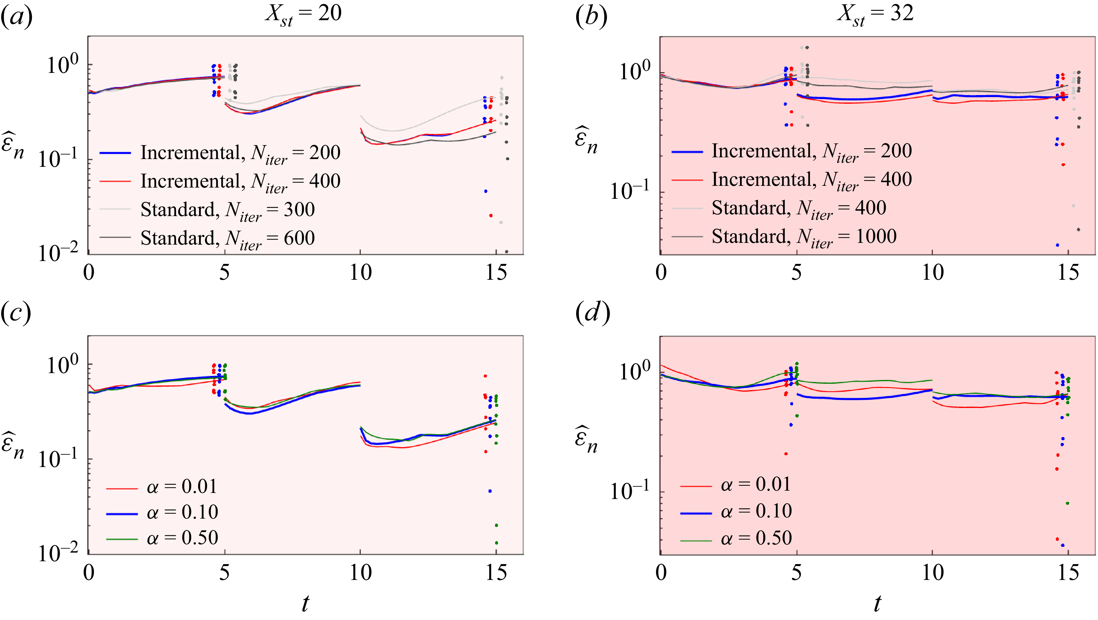
The evolution of
 $\widehat {\varepsilon }_n$
in a full field reconstruction of the KS system using 4D-Var; the scattered dots are
 $\varepsilon _n$
for the individual runs after the first and last sequences. The observations are at (a,c)
 $X_{\textit{st}}=20$
and (b,d)
 $X_{\textit{st}}=32$
, and at
 $(T_{\textit{st}},\sigma ) = (2,10^{-4}s_u)$
. (a,b) Comparison of the results from the incremental and standard approach at varying iteration numbers. (c,d) The independence of results to variation in regularisation parameter
 $\alpha$
.

Figures 12(a,b) show the results, over 10 independent runs, from incremental and standard approaches with varying
 $N_{\textit{iter}}$
for
 $X_{\textit{st}}=20$
and
 $X_{\textit{st}} = 32$
. The dark blue lines are the results presented in figure 2; other parameters here are the same as in figure 2. We find that the incremental approach is able to converge within
 $N_{\textit{iter}}=200$
, while the standard approach requires much higher iterations, particularly for the
 $X_{\textit{st}}=32$
case. Eventually, the two approaches are expected to converge to the same solution (Laroche & Gauthier Reference Laroche and Gauthier1998). Figures 12(c,d) are the results from the incremental approach with
 $N_{\textit{iter}} = 200$
but at varying regularisation parameter
 $\alpha$
. The results show that the optimisation is statistically independent of the value of
 $\alpha$
around the chosen value
 $\alpha =0.1$
for these cases. A much smaller
 $\alpha$
may not be able to regularise, while a much larger
 $\alpha$
may slow down the optimisation significantly.
Appendix C. Convergence issues in EnKF and 4D-Var
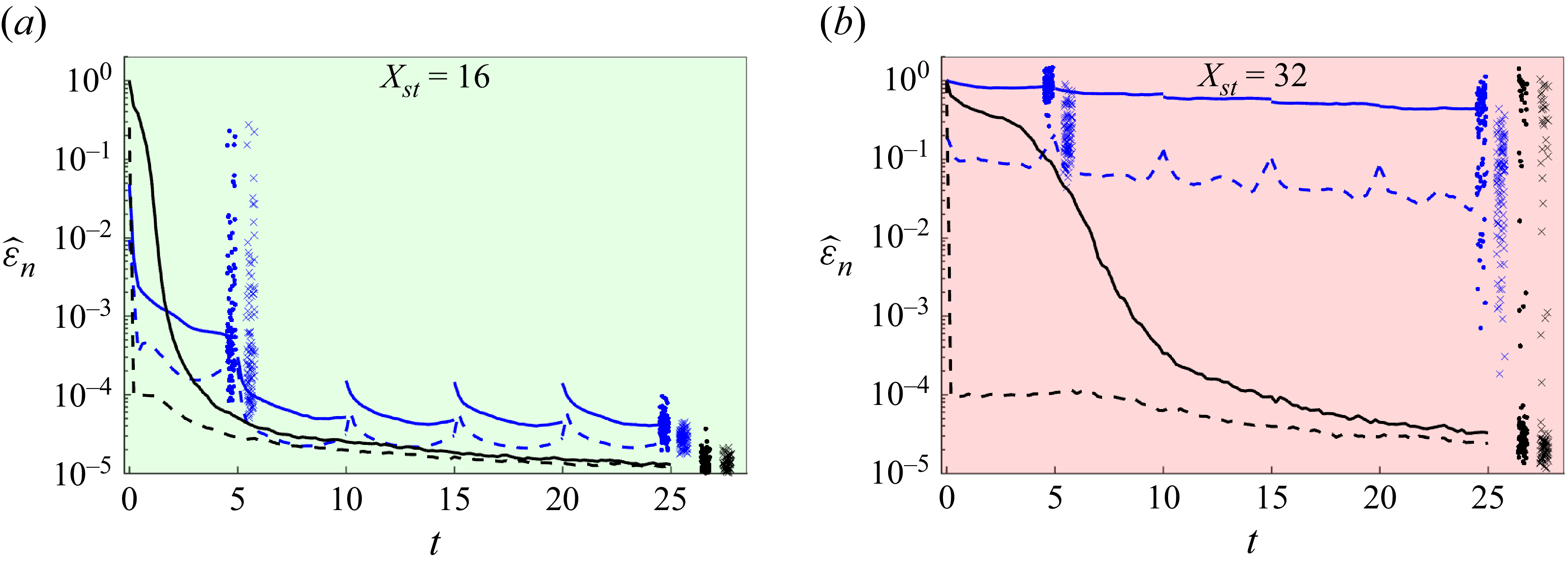
Figure 13 shows the same results as in the second and fourth panels of figure 2(a), i.e. the median estimation error
 $\widehat {\varepsilon }_n$
for the KS system at
 $X_{\textit{st}}=16$
and
 $X_{\textit{st}}=32$
using 4D-Var (blue) and EnKF (black). The solid lines and dots correspond to full field reconstruction errors, and dashed lines and crosses correspond to observation point errors. For the
 $X_{\textit{st}}=16$
case, the EnKF errors at the observation points rapidly come down to the noise level, while errors at the unobserved points slowly converge towards the observation point errors, and eventually both converge below the noise level for all the runs. The 4D-Var errors for the full field also closely follow the corresponding errors at observation locations, and both eventually converge below the noise level for all the runs. The difference between the solid and dashed blue lines (4D-Var), though insignificant, is still higher than that between the solid and dashed black lines (EnKF). This is because small-scale errors in EnKF analysis are smoothed out by the ensemble averaging. In contrast, for the
 $X_{\textit{st}}=32$
case, we find that the estimation errors for different runs vary over different orders of magnitude. This happens because of ensemble collapse in EnKF and local minima in 4D-Var, as explained below.
The evolution of
 $\widehat {\varepsilon }_n$
in estimating the KS system with (a)
 $X_{\textit{st}}=20$
and (b)
 $X_{\textit{st}}=32$
using 4D-Var (blue) and EnKF (black). The solid lines and dots correspond to full field reconstruction errors, and dashed lines and crosses correspond to observation point errors. For other parameters and figure details, see figure 2.

For the
 $X_{\textit{st}}=32$
case, the EnKF errors for most runs converge below the noise levels, but for many runs, the errors remain as high as
 $O(1)$
. In fact, for those high-error runs, even the estimation error at the observation points (black crosses) is of
 $O(1)$
. This happens because of errors in
 $\mathcal{B}_{\!j}^f$
leading to wrong corrections in the update step (see Appendix A). Such erroneous updates can cause all the ensemble members to divert away from the ground truth but come close to each other. If errors in
 $\mathcal{B}_{\!j}^f$
persist, then such erroneous updates will eventually bring all the ensemble members infinitesimally close to each other. Under such a situation, the Kalman gain
 $\mathcal{K}_{\!j}$
becomes too small to use the observations (see (2.6)) and the errors blow up everywhere, including at the observation points (Gottwald & Majda Reference Gottwald and Majda2013). To some extent, such an ensemble collapse can be avoided by introducing an inflation. We therefore use
 $\gamma =1.01$
for the
 $X_{\textit{st}}=32$
case.
For 4D-Var results for the
 $X_{\textit{st}}=32$
case, while the reconstruction error for a few runs has come down to
 $O(10^{-3})$
, it remains high for most runs. More importantly, we find that for most runs, there is a significant difference between the full field reconstruction error and the observation point errors (note that the observation point error is the 4D-Var cost function defined in (2.8)). Minimisation of the cost function relies on tangent linear hypothesis, which limits the size of the correction step at each iteration to the region of the linearisation validity. The limit on the correction step means that the optimisation may get stuck in a local minimum instead of reaching the optimal solution. The chances of that increase as the distance between the initial guess and optimal solution increases, such as with the increasing sparsity levels, and with nonlinearity in the system (Pires et al. Reference Pires, Vautard and Talagrand1996; Hoteit Reference Hoteit2008). When stuck in a local minimum, the cost function still reduces but the estimation stays far from the ground truth. This leads to the large difference between the full field and observation point errors. Hoteit (Reference Hoteit2008) suggests simulated annealing, in which several initial guesses are used to find the optimal solution, as a method to partially overcome this problem.