





1. Introduction
Recent radio observations have revealed a rich diversity in behaviour from the population of eruptive transients known as classical novae (CNe; Chomiuk et al. Reference Chomiuk, Metzger and Shen2021a, Reference Chomiukb). A classical nova is a thermonuclear transient in a compact, accreting binary system known as a cataclysmic variable. In a semi-detached binary system of a white dwarf and a companion star, when the companion star overflows the Roche lobe, it starts to transfer its hydrogen-rich material through the inner Lagrangian point (L1). These materials accumulate on the surface of the white dwarf, and as the temperature and density increase, the innermost layer soon becomes degenerate. These conditions trigger an unstable thermonuclear runaway, igniting thermonuclear fusion (Starrfield et al. Reference Starrfield, Truran, Sparks and Arnould1978). The outflow velocities from the white dwarf are typically in the range of hundreds to several thousand kilometres per second (Gallagher & Starrfield Reference Gallagher and Starrfield1978). The total energy output ranges from 1038 to 1044 erg, enriching the surrounding interstellar medium with heavier materials (Romano et al. Reference Romano, Matteucci, Zhang, Papadopoulos and Ivison2017).
Following the peak optical brightening at the mass ejection stage (Knigge et al. Reference Knigge, Baraffe and Patterson2011), the remnant envelope continues to support the nuclear burning, resulting in multi-component emission with complex radio light curves at different frequencies. Free-free thermal emission (Chomiuk et al. Reference Chomiuk2012) has traditionally been thought to dominate the radio emission from classical novae, but non-thermal synchrotron emission powered by the shock wave is now more commonly seen (Hernanz & Tatischeff Reference Hernanz and Tatischeff2012), especially from the gamma-ray producing novae studied by Ackermann et al. (Reference Ackermann2014), Chomiuk et al. (Reference Chomiuk, Metzger and Shen2021a). The evolution begins with the fireball expansion phase, during which the ejecta remain dense and optically thick due to absorption at all radio frequencies. During this phase, optically thick thermal emission from the photosphere dominates, resulting in a peak in the emission. The system becomes optically thin as density drops; that is, the photosphere recedes inward and traces the entire ejecta volume (Bode & Evans Reference Bode and Evans2012). The frequency at which the maximum amount of radiation escapes and the flux density drops further with expanding ejecta is called the turnover frequency. Following the peak, the flux density declines until the entire ejecta becomes fully transparent (Gulati et al. Reference Gulati2023).
Most radio studies of CNe today have been follow-up observations (Chomiuk et al. Reference Chomiuk2021b) of novae discovered at optical (or increasingly near-infrared; Lucas et al. Reference Lucas2020) wavelengths. This can yield high-quality multi-frequency observations but is limited to sources that have attracted specific interest from radio observers and may also be biased toward novae that peak sooner (otherwise, follow-up efforts may cease). However, with the advent of high-cadence wide-field radio surveys (Murphy & Kaplan Reference Murphy and Kaplan2026), serendipitous nova observations can cover a wider range of sources (e.g. Gulati et al. Reference Gulati2023), albeit often lacking multi-frequency coverage. In this paper, we use the first 3.5 yr of the Australian SKA Pathfinder (ASKAP; Hotan et al. Reference Hotan2021) Variables and Slow Transients (VAST; Murphy et al. Reference Murphy2013, Reference Murphy2021) survey data covering the Galactic plane at 2 week cadence to identify and study a flux-limited sample of classical novae. The paper is organised as follows. Section 2 outlines the source selection and summarises background information for the detected novae. Section 3 describes our approach to radio emission modelling, considering several emission models. In Section 4 we present the results of the light curve modelling. Finally, Section 5 summarises the findings with the conclusion presented in Section 6.
1.1. The ASKAP variables and slow transients survey
ASKAP is a radio survey telescope operating with 36 antennas with a total instantaneous field of view ≈31 deg2. The VAST survey conducted with ASKAP covers 1 200 deg2 of the southern Galactic plane every two weeks with an integration time ∼12 to 15 min per pointing. The typical rms noise is 0.2 mJy with central frequency 887.5 MHz and bandwidth 288 MHz. These high-cadence observations are optimised for monitoring transient and variable sources on timescales ranging from seconds to years. Data for individual sources are collected and calibrated as part of the VAST pipeline (Pintaldi et al. Reference Pintaldi, Stewart, O’Brien, Kaplan, Murphy, Ruiz, Pierfedereci and Teuben2022). Raw observational data for radio light curves are available in CASDAFootnote a
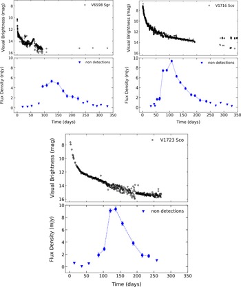
Optical (top) and radio (bottom) light curves for V6598 Sgr, V1716 Sco, and V1723 Sco. Optical data are from AAVSO; radio data at 887.5 MHz are from ASKAP VAST. Triangles indicate 5σ upper limits.

2. Sample selection
To search for classical novae, we began with the publicly available updated ‘Koji’s list of recent Galactic Novae’,Footnote b which compiles spectroscopically confirmed novae across the Galactic plane since 2008. The novae are grouped by the year of their earliest detected optical eruption. As of the last update at the time of writing (2026 January 6), the catalogue contains approximately 188 confirmed novae, with the most recent detection on 2025 November 29. We cross-matched the novae with ASKAP VAST survey data processed through the VAST pipeline using a 5 arcsec matching radius (Gulati et al. Reference Gulati2023), and searched for detectable radio emission for each candidate.
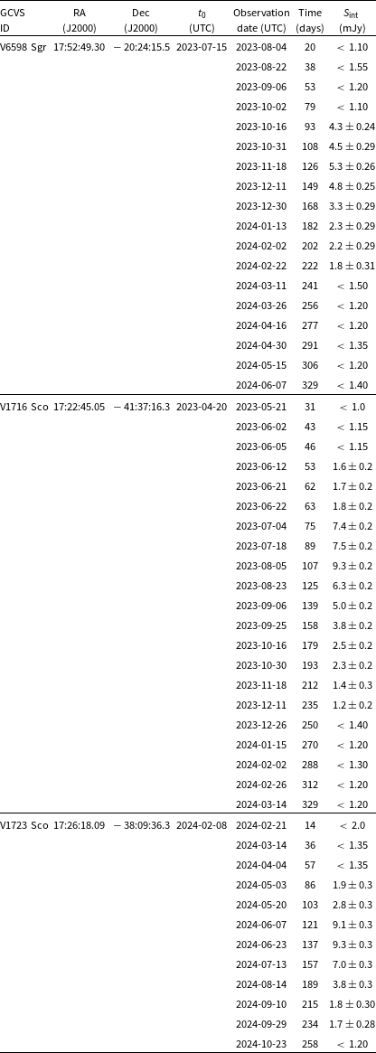
The VAST survey commenced on 2022 January, and our nova sample includes 43 Galactic novae reported between 2021 September 10 (≈100 days before 2022 January) and 2025 November 29, of which 32 fell within the VAST Galactic survey footprint and were searched for radio emission. Among these, three of the classical novae showed well-sampled flux density evolution (discussed in detail below), while the remaining 29 were consistent with non-detections (or one or two points above the noise floor, insufficient for detailed analysis). The radio data on the detected sources are listed in Table 1. Optical light curves were produced by using the American Association of Variable Star Observers (AAVSO) Database in the Johnson V or Visual band, given by Percy & Mattei (Reference Percy and Mattei1993). Radio and optical light curves are shown together in Figure 1, where we have taken the literature-reported discovery date as t 0. In the next sections, we summarise the previously reported multi-wavelength observations of individual novae, focusing on the most recent eruptions and data relevant to our modelling and interpretation.
2.1. V6598 Sgr
V6598 Sgr was reported in the visible band by Andrew Pearce and Y. Nakamura (Pearce et al. Reference Pearce2023b) on 2023 July 15, following a rapid rise of > 3 mag within < 24 h. Around the same time, it was detected by the Fermi Gamma-ray Observatory. The initial brightness was already near the maximum of 10 mag (Munari et al. Reference Munari2023) and dropped to 12.5 mag in ∼ 2 days (Pearce et al. Reference Pearce2023a). Spectral analysis detected broad Hα emission with a maximum projected velocity 4 000 km s−1 and from P-Cyg absorption line 3 500 km s−1 decreasing from 3 700 to 3 300 km s−1, leading to a classification as a fast nova with powerful ejecta with following a deceleration (Munari et al. Reference Munari2023).
ASKAP observations of classical novae from the VAST survey. Column 1 gives the General Catalogue of Variable Stars (GCVS) ID (Duerbeck Reference Duerbeck1981) of the novae. Columns 2 and 3 are right ascension and declination. Column 4 is the discovery date, which we considered as t 0 in optical detection. Column 5 contains the date of radio observations conducted with ASKAP, and Column 6 contains the number of days from the detection date. Column 7 gives the integrated flux density in mJy for ≥ 5σ detections or the 5σ upper limit.

Table 1. Long description
Panel A: Table with columns for General Catalogue of Variable Stars (GCVS) ID, right ascension, declination, discovery date, radio observation date, days from detection, and integrated flux density. Panel B: Graphs showing radio and optical light curves for detected novae, with axes labeled in days and flux density or magnitude units.
X-ray observations were obtained by Hare et al. (Reference Hare2021) using the Neil Gehrels Swift Observatory (Gehrels et al. Reference Gehrels2004). Based on these observations, the system was classified as an intermediate polar. The early evolution of V6598 Sgr shows similarities to two other He/N novae, V2672 Oph (Nova Oph 2009) and U Sco (Munari et al. Reference Munari2023). X-ray emission from U Sco resumed after ∼ 9 days of optical outburst, whereas V6598 Sgr re-emerged in X-rays after ∼ 17 days, suggesting that this is a magnetic binary system in which the accretion process resumed after its optical discovery (Nesci & Fiocchi Reference Nesci and Fiocchi2023).
Radio emission from V6598 Sgr was observed repeatedly from 2022 November 14 to 2024 October 10 at 887.5 MHz in the VAST survey and reported by Dobie et al. (Reference Dobie, Rose, Kaplan and Sivakoff2023). The source was detected above the ≥ 5σ upper limit in 8 epochs between 2023 October 16 and 2024 February 22. It was subsequently detected at 944 MHz on 2024 January 15 and 26 by Rose et al. (Reference Rose, Dobie, Murphy and Driessen2025) in the Rapid ASKAP Continuum Survey (RACS; McConnell et al. Reference McConnell2020). A steady increase in flux density from 4.3 ± 0.2 to 5.3 ± 0.2 mJy between day 93 and 126 was observed (Dobie et al. Reference Dobie, Rose, Kaplan and Sivakoff2023).
The geometric (purely parallax-based) and photogeometric (including priors to account for Lutz-Kelker bias; Lutz & Kelker Reference Lutz and Kelker1973) distances are
 $5.8_{-1.97}^{+1.96}$
and
 $4.3_{-1.18}^{+1.92} $
kpc (Bailer-Jones et al. Reference Bailer-Jones, Rybizki, Fouesneau, Demleitner and Andrae2021b) respectively, neither of which is statistically significant, and where the priors used for those photogeometric distances are not necessarily appropriate for CNe. In a recent study by Schaefer (Reference Schaefer2025), the distance of V6598 Sgr is estimated to be 7.661 kpc based on the Bayesian distance analysis (Schaefer Reference Schaefer2022), which uses Gaia parallaxes together with priors appropriate for Galactic nova populations and previous distance estimates with uncertainties. In this work, we use a distance of 7.6 kpc for our further model fitting and parameter estimations.
2.2. V1716 Sco
V1716 Sco was discovered by Pearce et al. (Reference Pearce2023a) on 2023 April 18 and 19 with a rapid rise from 12.5 to 7.3 mag within two days (Sokolovsky et al. Reference Sokolovsky2023). Later, it decreased by 2–3 mag in the next 15–20 days, making it a very fast nova according to the speed classes of classical novae (Strope et al. Reference Strope, Schaefer and Henden2010). Between 150 and 200 days, the visual brightness settled at 14–15 mag and returned to its quiescent state. V1716 Sco hosts a massive white dwarf of
 $1.21\,{\rm M}_{\odot }$
with a main-sequence star as donor (Schaefer Reference Schaefer2025), exhibiting typical behaviour of fast novae (Kato Reference Kato, Gänsicke, Beuermann and Reinsch2002). This is confirmed as a Fe II classical nova by spectroscopic analysis (Woodward et al. Reference Woodward, Shaw, Starrfield, Evans and Page2024). Spectra obtained by the Southern Spectroscopic Observatory Project (2SPOT) revealed complex and strong Balmer P-Cyg absorption lines with velocities of 1 800 km s−1 using the Deep Sky Chile Telescope (Pearce et al. Reference Pearce2023a).
After the optical outburst, X-rays and gamma-rays were detected within a day by NICER, NuSTAR, and Fermi-LAT (Sokolovsky et al. Reference Sokolovsky2023). The X-ray was observed from an optically thin thermal plasma heated by shocks, with a peak at ∼ 20 days after the eruption, entering the super soft (SSS) phase about 55 days later. Consistent with behaviour observed in many classical novae, detection of early X-rays and γ-rays implies a slow, low-density outflow dominated by a faster and denser wind, producing shocks (Wang et al. Reference Wang, Yan, Takata and Lin2024). During the SSS phase Worley et al. (Reference Worley2025) reported a 78 s quasi-periodic oscillation in X-rays with NICER, indicating variability in the emitting region with ongoing nuclear burning. From recently released Transiting Exoplanet Survey Satellite archival data, the orbital period is measured to be 1.36 days following an exceptionally low ratio of P spin/P orb = 6.6 × 10⁻⁴ (Luna et al. Reference Luna, Dobrotka and Orio2025).
V1716 Sco was observed in multiple epochs between 2022 November 19 and 2024 October 3 as part of the VAST survey. Significant radio emission was detected in 13 epochs between 2023 June 12 and 2023 December 11 (Anumarlapudi et al. Reference Anumarlapudi2023). The radio flux density rose rapidly, reaching a peak of 9.3 ± 0.2 mJy on day 107, before declining. The optical peak precedes the radio rise by 60–70 days. The geometric and photogeometric distances (Bailer-Jones et al. Reference Bailer-Jones, Rybizki, Fouesneau, Demleitner and Andrae2021a) are
 $3.19_{-1.62}^{+2.96}$
and
 $4.96_{-1.06}^{+1.75}$
kpc respectively (Wang et al. Reference Wang, Yan, Takata and Lin2024). Based on the Bayesian distance analysis of Schaefer (Reference Schaefer2025), which includes available Gaia information along with other data specific to novae, the reported distance for this source is 2.914 kpc, which is close to the geometric estimate of Bailer-Jones et al. (Reference Bailer-Jones, Rybizki, Fouesneau, Demleitner and Andrae2021a). Given the large uncertainty, we adopted a distance of 3 kpc. However, we also evaluated how the inferred parameters scale with distance to highlight the uncertainty.
2.3. V1723 Sco
V1723 Sco was discovered on 2024 February 8 (Sokolovsky et al. Reference Sokolovsky2024) with rapidly rising brightness, reaching a maximum value of 6.77 mag in V-band (Habtie & Das Reference Habtie and Das2024) within a few days of the optical eruption. At the time of discovery, the visual brightness was still increasing, and by day ∼ 4 it had declined to 8.1 mag, remaining at that level for the next few days. From the two optical spectra reported by 2SPOT on 2024 February 11 and 12, the nova shell appear to be still expanding at 3 200 km s−1 (Hα line) and 1 800 km s−1 (Hβ line) respectively (Habtie & Das Reference Habtie and Das2024).
Gamma-ray emission above 100 MeV was detected starting on 2024 February 9 (Cheung Reference Cheung2024). The follow-up observations revealed an average photon flux of (1.9 ± 0.5) × 10−6 photons cm−2 s−1 on 2024 February 11–12, ∼ 2–3 days after the outburst. The typical range of photon flux for classical novae reported by Fermi-LAT is 10−7 photons cm−2 s−1 (Ackermann et al. Reference Ackermann2014). Novae such as V1324 Sco (Finzell et al. Reference Finzell2018), V5668 Sgr (Cheung et al. Reference Cheung2016) are example of the brighter end of this population. Only a few classical novae including V407 Cyg (Abdo et al. Reference Abdo2010), V959 Mon (Hachisu & Kato Reference Hachisu and Kato2018) have reached such brightness (10−6 photons cm−2 s−1) similar to V1723 Sco. Therefore, this is one of the strongest and most luminous gamma-ray-detected classical novae since 2010 (Cheung & Jean Reference Cheung and Jean2024). This source was observed from February 10.299–11.767 UT in hard X-rays by NuSTAR and in soft X-rays by Swift/XRT, up to February 13, with both showing non-detections (Sokolovsky et al. Reference Sokolovsky2024). Later, on 2024 March 13 (33 days from the optical outburst), it reached its peak in the soft band (0.3–2 keV), and became one of the highest level of shock-powered classical novae to reach such X-ray brightness (Fauverge et al. Reference Fauverge2026).
Radio observations of V1723 Sco started on 2024 February 17 using the Karl G. Jansky Very Large Array Telescope with a magnitude of 7.8 mJy (Molina et al. Reference Molina2024b). The calculated spectral index from multi-frequency data is α = 0.5, suggesting an optically thick phase in its radio flux evolution. For V1723 Sco we used a distance of ∼ 8 kpc from Schaefer (Reference Schaefer2025), adopting the Bayesian analysis from Schaefer (Reference Schaefer2022). From 2024 February 21 to April 4, ∼ 14 to 57 days after the eruption, this classical nova candidate remained undetected with a 3σ upper limit in all available epochs of the VAST survey. The first detection by ASKAP was made 86 days post-eruption, on 2024 May 3, at 1.9 ± 0.3 mJy. The source peaked on day 137 and was last detected at 1.7 ± 0.28 mJy, after which it became undetected.
3. Analysis and modelling
To fit the data, we considered both thermal (bremsstrahlung) (Hjellming et al. Reference Hjellming, Wade, Vandenberg and Newell1979; Osterbrock Reference Osterbrock1989) and non-thermal (magnetobremsstrahlung) (Chevalier Reference Chevalier1998; Nyamai et al. Reference Nyamai2023) emission models. To estimate the uncertainties in flux density, we used the quadrature sum of the local RMS, peak-flux error, and 10% flux-scaling error, following McConnell (Reference McConnell2015). For quantitative assessment of the quality of each fit, we used the Akaike Information Criterion (AIC; Tan & Biswas Reference Tan and Biswas2012) and the Bayesian Information Criterion (BIC; Liddle Reference Liddle2007). Here, we briefly discuss each of our emission models. We present one corner plot for each source with the lowest reduced χ 2 value, which also corresponds to the lowest AIC and BIC values.
3.1. Free-Free thermal emission
After the nova eruption, radio emission may arise from the hot, ionised plasma undergoing Hubble-type expansion away from the white dwarf. The intensity of this emission depends on the electron temperature and plasma density. The radio light curve represents the evolution of the optical depth τ ν along with the expansion of the ejecta. It initially rises during an optically thick phase (τ ν ≫ 1), reaches a peak when the optical depth of the ejecta approaches unity, and then declines further as the ejecta expands (τ ν ≪ 1) and becomes optically thin (Osterbrock Reference Osterbrock1989; Seaquist Reference Seaquist, Bode and Evans2008; Hopkins et al. Reference Hopkins2003). We adopted the standard free-free thermal model with a linear velocity gradient for the nova shell, as given by Hjellming et al. (Reference Hjellming, Wade, Vandenberg and Newell1979). The free parameters are the ejecta mass M ej, inner and outer velocities v 1 and v 2, inner and outer radii r 1 and r 2, and electron temperature T e. In the optically thin limit, the free-free flux density can be defined as,
 \begin{align} S_{\nu _{{\rm thin}}}=C \left [\frac {M_{{\rm ej}}^2}{d^2\ \!r_2\ \!r_1\,(r_2-r_1)}\right ] \end{align}
where the coefficient C is;
 \begin{align} C = \frac {J_0}{4\pi\ \!m_p^2}\, T_e^{-0.5}\, g_{ff}\, \exp \left [-\frac {h\nu }{k_B T_e}\right ] \end{align}
In the expression above, J 0 is the free-free normalisation constant and g ff is the free-free Gaunt factor, both defined from Osterbrock (Reference Osterbrock1989), and m p is the proton mass. Considering T e = 104 K and ν = 887.5 MHz, the value of this constant in cgs unit is C = 9.32 × 10⁶ erg s−1 Hz−1cm3 g−2. In the light curve fitting, we used the full expression, including free-free self-absorption, allowing the model to transition between optically thick and optically thin regimes. For Hubble-like expansion r 1 and r 2 are given by:
 \begin{align} r_1 = r_{10} + v_1(t-t_0) \end{align}
and
 \begin{align} r_2 = r_{20} + v_2(t-t_0) \end{align}
At a time t compared to the eruption time t 0. At t 0 = 0, the initial radii of the ejected shell are r 10 and r 20, although we ignore these in subsequent analysis (since the radio emission is at a late time with r ≫ r 0). We fixed the electron temperature at 104 K since the dependence of the emission on T e is very weak when just dealing with a single radio frequency.
The model then becomes a three-parameter model with parameters M ej, v 2, and v 1/v 2. We fit the data with the MCMC method by using the emcee package (Foreman-Mackey et al. Reference Foreman-Mackey, Hogg, Lang and Goodman2013). Based on the parameter values commonly reported in previous studies of classical novae, as referenced above, we set the priors as; 10−7 M⊙ < M ej < 10−4 M⊙, 100 km s−1 < v 2 < 10 000 km s−1, and 0.4 < v 1/v 2 < 0.8. Our fits used 60 walkers over 1 000 steps. We produced corner plots to visualise the posterior distributions and best-fit values with uncertainties, and used them to generate sample models for visual comparison with the observational data.
3.2. Non-thermal synchrotron emission
When the fast, rapidly expanding ejecta interact with slower, less dense circumbinary material, it generates a shock wave (Borkowski et al. Reference Borkowski, Blondin and Sarazin1992) at the interface of the two media. The interaction between the faster ejecta and the earlier and slower outflow from the white dwarf surface concentrated at the equatorial plane of the binary produces internal shocks typically observed in classical novae (Metzger et al. Reference Metzger2014). The collision between fast ejecta and dense stellar wind from the companion produces external shocks associated with symbiotic and recurrent novae (Vlasov et al. Reference Vlasov, Vurm and Metzger2016). Both shock waves carry the energy of the outburst and transfer a fraction (
 $\epsilon_{\textrm{e}}$
) of this energy to accelerate electrons to relativistic speeds and a fraction (
 $\epsilon$
B) to amplify the magnetic field. Non-thermal synchrotron emission arises when these relativistic electrons spiral along magnetic field lines. This energy transfer process follows a power-law energy distribution: N(E) dE ∝ E
−p
dE. Therefore, the light curve evolves based on the circumbinary density, the magnetic field strength, the change in optical depth because of self-absorption (SSA; Chevalier & Fransson Reference Chevalier and Fransson1994) or free-free absorption (FFA), the geometry of the ejecta, and the area of the emitting region (Chevalier Reference Chevalier1998).
From the point of discontinuity, the forward shock propagates outward, and the reverse shock propagates inward through the faster ejecta. The synchrotron-emitting region lies within this shock and the contact discontinuity, with a volume-filling factor f ≤ 1. Emission from the reverse shock is usually absorbed by the cold central shell (Vlasov et al. Reference Vlasov, Vurm and Metzger2016), which dominates at frequencies below some turnover. Above the turnover frequency, the light curve transitions from an optically thick to an optically thin phase τ ν ≪ 1. To fit this type of emission, we adopted the standard synchrotron model from Nyamai et al. (Reference Nyamai2023) and Chevalier (Reference Chevalier1998), where the surrounding material is approximated by an effective ρ(R) ∝ R −2 density profile, with R being the expanding shock front radius. In applying this model to classical novae, we interpret this density profile as an effective description of the slow ejecta or circumbinary material encountered by the shock. To further incorporate this emission mechanism, we considered both synchrotron self-absorption (SSA) and an external FFA factor. While SSA regulates within the shocked region, FFA from ionised material along the line of sight further suppresses the emission and delays the radio peak. Here, we applied an intrinsic SSA with an external FFA screen to model our observational data.
However, as we shall see, this single power-law model cannot explain the steep post-peak decline observed in these very fast, early synchrotron flares. Different classical novae exhibit distinct rise and decay slopes in their radio evolution, indicating that a single smooth density profile may not be sufficient to describe the effective density structure encountered by the shock. While some novae have been modelled with aspherical ejecta, for example, V959 Mon (Healy et al. Reference Healy, O’Brien, Beswick, Avison and Argo2017), RS Oph (Munari et al. Reference Munari2022), V445 Pup (Nyamai et al. Reference Nyamai2021), V407 Cyg (Pan et al. Reference Pan, Ricker and Taam2015), or with variations in filling factor, we needed a simpler approach given our limited single-frequency data. Therefore, to capture this complex, asymmetric temporal behaviour, we modified the density profile (ρ) of this shock-interacting material by introducing a broken power law. Hence, ρ falls at a different rate in two separate regions while maintaining a smooth, continuous transition, i.e. at R ≪ R 0 and R ≫ R 0, where R 0 is the characteristic scale radius or the break point of the two different regions. A simple broken power law for this surrounding density structure can be written as
 \begin{align} \rho \propto \left ( \frac {R}{R_0} \right )^{-k}\left \{\frac {1}{2}\left [1 + \left ( \frac {R}{R_0} \right )^{1/n}\right ]\right \}^{(k - m)n} \end{align}
We used three different power k, m, and n, where k controls the inner slope, i.e. how steeply the density drops at R ≪ R
0 region, n controls the transition smoothness or how abruptly the density profile turns over near the break radius R
0 and lastly m controls the steepness of post peak decay at large R (R ≫ R
0). Three sources showed different rates of steepness in their light curves. However, we did not fit for these indices, we fixed them at certain values depending on the steepness of temporal evolution as R(t) ∝ t then fit for five parameters such as filling factor f, wind velocity V
wind, mass-loss rate
 $\,\dot{\!M}$
, explosion energy E, ejected mass M
ej, via MCMC sampling. In this work, we considered the model parameter V
wind as the velocity of the slower circumbinary material that the shock encounters. We chose the fraction of energy transferred to electrons
 $\epsilon_{\textrm{e}}$
= 0.01 and the fraction of energy transferred to the magnetic field
 $\epsilon$
B = 0.01 and p = 2.5 for our calculations (Pacholczyk Reference Pacholczyk1970). The best-fit model was sampled with 100 walkers over 1 000 steps. Similarly based on the parameter values commonly reported in previous synchrotron emission studies of classical novae, as referenced above, the adopted priors for MCMC sampling are; 0.01 < f < 1, 50 km s−1 < V
wind < 400 km s−1, 10−7 M⊙ yr−1 <
 $\,\dot{\!M}$
< 10−4 M⊙ yr−1, 1042 erg < E < 1045 erg, and 10−7 M⊙ < M
ej < 10−4 M⊙. After the MCMC run, we took 100 samples with uncertainties and plotted them to visually compare with the data.
3.3. Distance scaling
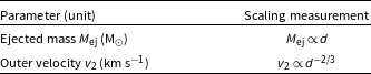
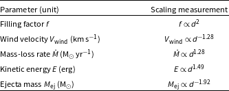
For each source, we computed the best-fit model for the nominal distances in Section 2. We did not allow the distance to be a free parameter in the fit, since the fitted parameters are highly degenerate with distance. However, since many of the distances we adopt are themselves highly uncertain, we provide the scaling factors for each fitted parameter with respect to distance. In general, the flux density will scale roughly as a power-law function of each parameter (at least when close to the best-fit values) and to compensate for the d −2 scaling of the flux density with distance, we derived the scaling indices that are listed in Tables 2 and 3.
Approximate power-law scaling indices for each parameter with distance d for the free-free emission model. We kept the electron temperature fixed at T e = 104 K.

Table 2. Long description
The table compares approximate power-law scaling indices for parameters with distance for free-free and synchrotron emission models. It has two sections: Table 2 for the free-free emission model and Table 3 for the synchrotron emission model. Table 2 has three rows and three columns. Column headers are Parameter (unit), Scaling measurement, and a third column with scaling indices. Row labels are Ejected mass Mej (M), Outer velocity v2 (km s1), and their respective scaling indices. Table 3 has five rows and three columns. Column headers are Parameter (unit), Scaling measurement, and a third column with scaling indices. Row labels are Filling factor f, Wind velocity Vwind (km s1), Mass-loss rate (M yr1), Kinetic energy E (erg), Ejecta mass Mej (M), and their respective scaling indices.
Approximate power-law scaling indices for each parameter with distance d for the synchrotron emission model, with electron power-law index fixed to p = 2.5.

Table 3. Long description
A table with two columns and four rows. The columns are labeled ’Parameter (unit)’ and ’Scaling measurement’. The rows are as follows: Row 1: Filling factor f, f d2; Row 2: Wind velocity Vwind (km s1), Vwind d1.28; Row 3: Mass-loss rate (M yr1), d1.28; Row 4: Kinetic energy E (erg), E d1.49; Row 5: Ejecta mass Mej (M), Mej d1.92.
We started by calculating the power-law indices analytically for each parameter as a function of distance. However, for parameters like E,
 $\,\dot{\!M}$
, V
wind, and M
ej in the synchrotron model, the model is not a pure power law. The distance-scaling exponent itself varies with distance. Therefore, we estimated the local exponent at the flux density peak (t
peak ≈100 days) by using the best-fit value and our reference distance.
4. Results
4.1. V6598 Sgr
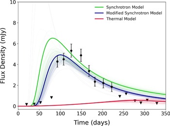
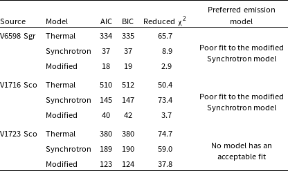
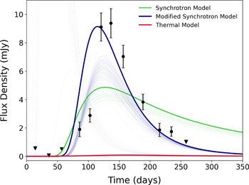
We statistically compared the fit of all three models shown in Figure 2 and concluded that the modified synchrotron model provides a comparatively better fit to the observed data, with a reduced χ 2 = 2.9 and 3 degrees of freedom. The best-fit values from MCMC analysis are listed in Table 6. The thermal model rises too slowly and remains faint during the observed radio maximum. It suggests that a single spherically symmetric, uniformly filled thermal shell is unlikely to capture the dominant emission mechanism in this source. Instead, the observed light curve is more consistent with a shock-powered synchrotron emission component whose visibility evolves as the ejecta and the surrounding material become optically thin at 887.5 MHz.
This result is consistent with the multi-frequency evidence for shocks in V6598 Sgr, including the short-lived Fermi-LAT detection, broad optical emission lines, and rapid early evolution. The radio emission peak indicates that the low-frequency synchrotron emission becomes visible on a ∼4 month timescale. From the light curve, we can observe that the transition from optically thick to thin is more gradual and smoother here than in the other two sources. In our synchrotron model, this behaviour is captured by the adopted density transition parameter n 0.7. This may indicate that the shock is propagating through a comparatively dense or smoothly varying environment, consistent with the gamma-ray interpretation that the accelerated particles may be located in a dense region (Fauverge et al. Reference Fauverge2026).
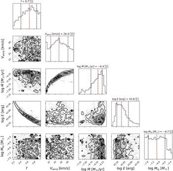
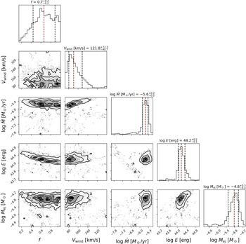
However, none of the models gives a satisfactory fit, and the posterior distribution in Figure 3 shows strong degeneracies among the physical parameters. Different combinations of explosion energy, ejecta mass, mass-loss rate, wind velocity, and density-profile shape can produce broadly similar light curve behaviour. Therefore, the fitted parameters should be interpreted cautiously.
Model fit of thermal, non-thermal, and modified non-thermal emission to V6598 Sgr at 887.5 MHz, with the red, green, and blue light curves representing the respective model fits. Spaghetti plots based on 100 posterior samples from MCMC fitting are shown to illustrate the spread and uncertainty of the model, while the bold curve denotes the best-fit model.

Best-fit parameters M ej, v 2, and v 1/v 2 that were directly sampled by the MCMC with the free-free thermal model. We kept the electron temperature T e fixed at 104 K. The inner velocity v 1 was not independently varied as a free parameter, but it was computed for each posterior sample by using v 1/v 2 with the uncertainty of this derived distribution. The best-fit value of M ej is mentioned on a log scale.

Table 4. Long description
A table comparing best-fit parameters for different sources. The table has three rows and seven columns. Column headers are Source, log Mej (M), v2 (km s1), v1/v2, v1 (km s1), Te (K), and d (kpc). Row 1: V6598 Sgr, 3.1 0.15, 9 800 200, 0.6 0.1, 6 300 1250, 104, 7.6. Row 2: V1716 Sco, 4.0 0.01, 9 300 530, 0.8 0.01, 7 330 440, 104, 3.0. Row 3: V1723 Sco, 4.1 0.16, 9 880 350, 0.7 0.1, 6 900 1 000, 104, 8.0.
This is the corner plot of V6598 Sgr, showing the posterior distribution of the five parameters fit with the modified synchrotron emission model. The parameters that we varied are filling factor f, wind velocity V
wind, mass-loss rate
 $\,\dot{\!M}$
energy E, ejected mass M
ej. This 2D contour plot corresponds to the best-fitting model among the three fits. The correlations between the parameters show that they are coupled and adjust accordingly to maintain the optical evolution.

4.2. V1716 Sco
V1716 Sco is a classical nova with significant gamma-ray detection. Following the typical classical nova structure, it contains a main-sequence star (Schaefer Reference Schaefer2025) as its companion. Therefore, the non-thermal emission from this source indicates internal shocks within the ejecta. The presence of this early radio synchrotron flare is consistent with other gamma-ray-detected novae. From Figure 1, we observed that within ∼110 days from the optical eruption, the radio flux rose very steeply and reached its peak, followed by a very steep post-peak decline. This rapid variability at the low frequency 887.5 MHz makes it a strong synchrotron-dominated source with almost no thermal emission in early times.
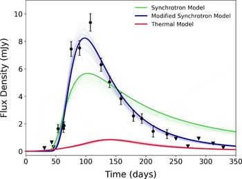
Figure 4 shows the model fits with uncertainties. As expected, the thermal model failed to estimate such a high flux density at a lower frequency, whereas the synchrotron models roughly estimated the observed values. Compared to other classical novae observed at the same frequency, 887.5 MHz, such as V1369 Cen, V5668 Sgr, RR Tel, and YZ Ret (Gulati et al. Reference Gulati2023), V1716 Sco shows much denser temporal sampling with multiple detections. This suggests that this source is highly luminous and produces very efficient particle acceleration. Since the shock propagates through a complex, non-uniform, steeply graded, dense circumbinary material, a wind-like density profile varying as R −2 is not sufficient to describe the evolution. Given that this binary hosts a main-sequence star, it can be assumed that this steep fall after the turnover frequency is due to the very low density of the ambient medium. That is, when the shock propagates through the R ≫ R 0 region, the density drops so abruptly that there are not enough electrons to be accelerated by the shock-carried energy. This lack of efficiently accelerated electrons causes the flux density to drop very rapidly. Even though none of the models has an acceptable fit based on the χ 2 value, the broken power-law model still provides a better fit and captures the steep decline. We modelled the radio light curves by fixing the slopes to k = 3.1 for the optically thick phase, m = 3.3 for the optically thin phase, and n = 2.7 for the transition between the two. From the fit, it is evident that both the rise (S ν ∝ t 3.1) and decay (S ν ∝ t −3.3) are far more rapid than expected for freely expanding, optically thick thermal ejecta, which scales as S ν ∝ t 2.
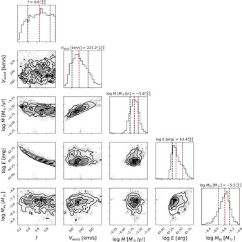
The best-fit values for all three models from the MCMC sampling are in Tables 4–6, and Figure 5 is the corner plot of the posterior distribution of our modified synchrotron model fit. The density profile in this model scales as
 $\rho$
∝
 $\,\dot{\!M}$
 $V_{\text{wind}}^{-1}$
, which means that a high mass-loss rate needs a higher wind velocity to match the temporal evolution. This explains the parameter degeneracy, contributes to poor constraints, and reduces the quality of the fit. Similarly, from Table 3, we could compute how the parameters will change if our adopted distance is not true.
The 2D corner plot in Figure 5 shows broad but correlated posterior distributions of f, V
wind,
 $\,\dot{\!M}$
, E, and M
ej. These degeneracies are expected due to the limited observational constraints. The fractional value f = 0.6 suggests the partial involvement of the shell in this non-thermal emission. Even though none of the fits was good, the comparison still favours a two-component shock scenario, in which a dense, fast flow collides with a slower, less dense environment, producing non-thermal synchrotron emission that dominates at low frequencies (Vlasov et al. Reference Vlasov, Vurm and Metzger2016).
Best-fit parameters f,
 $V_{\rm wind}$
,
 $\,\dot{\!M}$
, E, and
 $M_{\rm ej}$
that were directly sampled by the MCMC with the synchrotron emission model fit. We kept a fixed value of p = 2.5, and
 $\epsilon$
e =
 $\epsilon$
B = 0.01 and distance d according to the source. The best-fit values of
 $\,\dot{\!M}$
, E, M
ej parameters are in log scale.

Table 5. Long description
A table comparing best-fit parameters for synchrotron emission model fits across different sources. The table has 3 rows and 12 columns. Column headers are: Source, f, Vwind (km s1), log (M yr1), log E (erg), log Mej (M), p, e, B, d (kpc), k, m, n. Row 1: V6598 Sgr, 0.6, 0.2, 6.3, 0.4, 43.5, 0.2, 5.8, 0.6, 2.5, 0.01, 0.01, 7.6, 2.4, 2.5, 0.7. Row 2: V1716 Sco, 0.7, 0.2, 213, 110, 5.9, 0.2, 43.0, 0.1, 5.9, 0.3, 2.5, 0.01, 0.01, 3.0, 3.1, 3.3, 2.7. Row 3: V1723 Sco, 0.7, 0.2, 5.5, 0.2, 43.6, 0.2, 5.6, 0.5, 2.5, 0.01, 0.01, 8.0, 3.1, 3.6, 3.0.
In this table the best-fit parameters f, V
wind,
 $\,\dot{\!M}$
, E, and M
ej were listed from the modified synchrotron emission model fits.
 $\,\dot{\!M}$
, E, M
ej are listed in log scale. Here, we kept p,
 $\epsilon$
e, and
 $\epsilon$
B at values similar to those of the previously fitted standard synchrotron model. However, from the broken power law radial function in ρ profile, we now fixed three new indices k (controls inner slope), m (controls outer slope), n (transition rate) with different values based on the rise and decay slopes. We assigned these powers individually to the source, as each showed a different temporal behaviour. For example, at early times, V6598 Sgr had a typical value of t
−2 in its slope, whereas V1716 Sco and V1723 Sco varied much more steeply at ≈t
−3.1. We can clearly observe this rapid variability in their light curves before even applying any model.

Table 6. Long description
A table with five rows and five columns. The columns are labeled Parameter (unit), Scaling measurement, and the rows are labeled with different parameters and their scaling measurements. Row 1: Parameter (unit): Filling factor f, Scaling measurement: f ∝ d^2. Row 2: Parameter (unit): Wind velocity V_wind (km s^-1), Scaling measurement: V_wind ∝ d^-1.28. Row 3: Parameter (unit): Mass-loss rate \.M (M_\odot yr^-1), Scaling measurement: \.M ∝ d^1.28. Row 4: Parameter (unit): Kinetic energy E (erg), Scaling measurement: E ∝ d^1.94. Row 5: Parameter (unit): Ejecta mass M_e (M_\odot), Scaling measurement: M_e ∝ d^-1.92.
Radio light curve fitting of V1716 Sco for thermal, non-thermal, and modified non-thermal emission models. Red, green, and blue curves show three different models. From the MCMC posterior distribution, 100 samples are used to generate a spaghetti plot illustrating the uncertainty ranges, with bold lines indicating the respective best-fit solutions.

4.3. V1723 Sco
We applied the same three models to this newly observed source, as illustrated in Figure 6. Gamma-ray and X-ray studies indicated this as a very powerful shock-driven non-thermal synchrotron flare with efficient particle acceleration. The flux density rises steeply from 2.8 ± 0.3 to 9.3 ± 0.3 mJy. This rapidly evolving synchrotron flare, spanning ∼ 150 days, has no acceptable fit with any of our models. The fitting results are presented in Table 7. The posterior distributions for the broken powe-law synchrotron model are shown in Figure 7. The basic non-thermal model was unable to produce these sharp slopes and failed to account for the short-lived peak. In our broken power-law model, we varied k, m, and n over a realistic range of 1 − 4 to see whether it could produce such steep changes. Later, we set k = 3.1, m = 3.6, and n = 3 for the fitting, but it still failed to match the peak and yielded unsatisfactory χ 2 values. This temporal change S ν ∝ t −3.6 in flux density is much higher than that of a typical thermal-dominated classical nova, decaying as S ν ∝ t −2, supporting it as a very bright, luminous, and strong synchrotron emission source with significantly efficient particle acceleration.
Posterior distribution of the parameters in the broken power-law synchrotron model fit to V1716 Sco. These parameters are poorly constrained, resulting in a poor fit to the data. Mass-loss rate
 $\,\dot{\!M}$
and wind velocity V
wind showed a positive correlation, reflecting the model degeneracy to sustain the observed radio flux, maintaining the
 $\rho \propto \frac {\dot M}{V_{{\rm wind}}}$
density profile. While the energy and filling factor showed negative correlations, implying that if we make the shock more energetic, we need a smaller filling factor to produce the same radio flux peak.

The V-band data show some irregularity around the rise and peak epochs of this radio flare. However, we do not interpret this as definitive evidence of correlated optical-radio variability. We note that a recent study of the Fermi-LAT gamma-ray observation of V1723 Sco by Fauverge et al. (Reference Fauverge2026) supports the presence of shock activity in this system. A possible late-time high-energy activity is mentioned there, which could indicate continued particle acceleration, potentially associated with hot materials heated by a new shock. This shows that V1723 Sco was a shock-active system and not evolving toward a simple spherically symmetric photosphere. Energy injections into the ejecta can also exhibit variability and randomness, which can cause the ejecta to react more violently and generate stronger internal shocks (Chomiuk et al. Reference Chomiuk2021b). Taken together, this supports the idea of an early synchrotron flare arising when the nova is still re-energising or reshaping the entire outflow structure.
5. Discussion
We modelled the light curves of these novae using two emission mechanisms commonly observed in classical novae: thermal free-free emission (Hjellming et al. Reference Hjellming, Wade, Vandenberg and Newell1979) and non-thermal synchrotron emission (Chevalier Reference Chevalier1998; Nyamai et al. Reference Nyamai2023). Again, in contrast to previous works, where identification of non-thermal emission was based on spectral information (Molina et al. Reference Molina, Chomiuk and Linford2024a; Weston et al. Reference Weston2016a, Reference Westonb; Nyamai et al. Reference Nyamai2021) or brightness temperature measurements (Chomiuk et al. Reference Chomiuk2021b), here we attempted to identify the dominant emission mechanism based on the light curve shape. We adopted a broken power-law in the synchrotron emission model to incorporate non-uniform shock-evolution dynamics and referred to it as the modified synchrotron emission model. For all three novae, the free-free thermal model under-predicts the flux density and was not able to describe the observed light curve. The synchrotron model over-predicted the flux and failed to reproduce the temporal evolution. For these sources, the modified synchrotron model provides a better fit than the thermal or standard synchrotron models. Although none of the models has a formally acceptable fit, this model with a broken power-law density profile yielded the lowest χ 2 among the three. This early synchrotron flux depends primarily on the density of the circumbinary material and on how the faster ejecta interacts with the lower, less dense material, producing internal shock waves driven by the sharp velocity and density gradient. All these systems have an MS as their companion (Schaefer Reference Schaefer2025), which implies a tenuous circumbinary medium. Due to the absence of a dense circumstellar medium, the duration of this early flare is very rapid and short-lived. Therefore, the steep post-decay observed in these sources is likely because, as the wave propagates into a much lower-density medium, it encounters no electrons in front of it to accelerate. In this work, we adopted a simple spherically symmetric model, whereas nova ejecta are far more complex in density structure and morphologies. Radio observations (Chomiuk et al. Reference Chomiuk2021b) of systems such as V745 Sco (Molina et al. Reference Molina, Chomiuk and Linford2024a), V445 Pup (Nyamai et al. Reference Nyamai2021), V1723 Aql (Weston et al. Reference Weston, Woudt and Ribeiro2014) revealed complex mass loss behaviour, including rapid variability and multiple peaks in their radio light curves. Therefore, the flux density evolution of these systems cannot be reproduced by a single thermal or non-thermal emission model. Future multi-frequency radio observations combined with improved distance constraints and more physically realistic shock models will be essential for better constraining emission dynamics and particle acceleration processes in these systems.
Model comparison statistics for each nova. Lower χ ν 2, AIC, and BIC values indicate a better fit. Based on their calculated values, the preferred model is mentioned. V1723 Sco had no acceptable fit with any of the models. Therefore, we are unable to identify the preferred model for this source.

Table 7. Long description
A table comparing model statistics for different nova sources. The table has 12 columns and 3 rows. Column headers are Source, f, V_wind (km s^-1), log \.M (M_\odot yr^-1), log E (erg), log M_ej (M_\odot), p, \epsilon_e, \epsilon_B, d (kpc), k, m, n. Row 1: V6598 Sgr, 0.7 ± 0.2, 26 ± 14, -6.4 ± 0.3, 43.6 ± 0.1, -6.7 ± 0.9, 2.5, 0.01, 0.01, 7.6, 2.4, 2.5, 0.7. Row 2: V1716 Sco, 0.6 ± 0.3, 221 ± 64, -5.6 ± 0.1, 43.4 ± 0.2, -5.5 ± 0.3, 2.5, 0.01, 0.01, 3.0, 3.1, 3.3, 2.7. Row 3: V1723 Sco, 0.7 ± 0.2, 122 ± 56, -5.6 ± 0.2, 44.2 ± 0.2, -4.8 ± 0.4, 2.5, 0.01, 0.01, 8.0, 3.1, 3.6, 3.0.
Radio light curve fitting of V1723 Sco for thermal, non-thermal, and modified non-thermal emission models. Red, green, and blue curves show three different models. From the MCMC posterior distribution, 100 samples are used to generate a spaghetti plot illustrating the uncertainty ranges, with bold lines indicating the respective best-fit solutions.

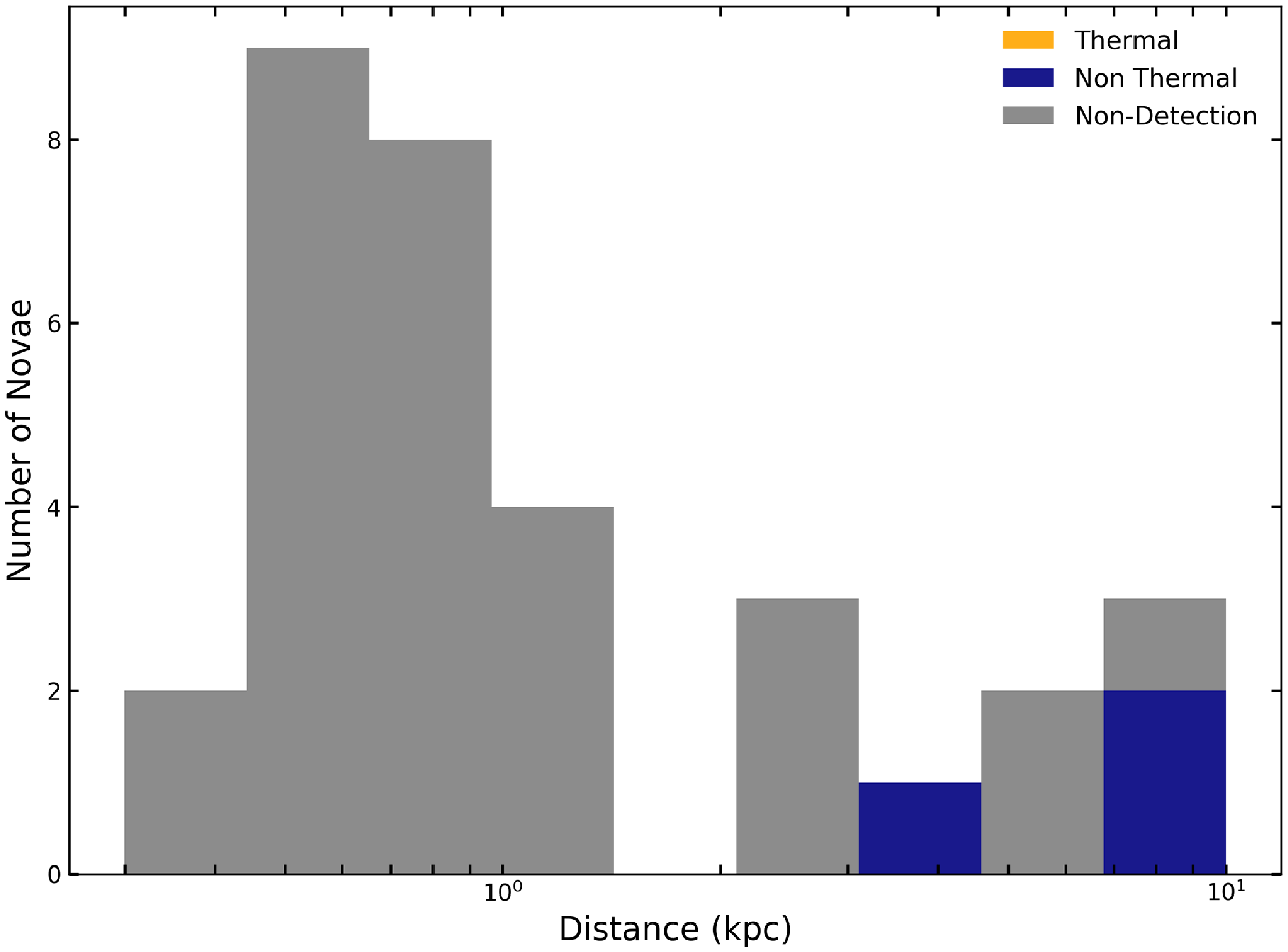
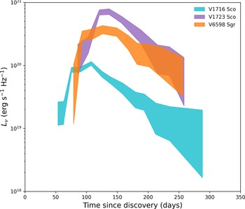
In Figure 8, we present the distribution of classical novae as a function of distance. From the literature survey, we find that most novae within 1 − 2 kpc remained undetected by ASKAP VAST. This may be partly explained by our observing frequency of 887.5 MHz. At this low frequency, many nearby novae are not detected because they remain optically thick, with the radio emission suppressed by free-free or SSA. Therefore, we see that classical novae detected by ASKAP VAST within approximately 100–150 days after eruption exhibit relatively early, low-frequency radio emission, compared with many thermally dominated nova light curves, which can peak on much longer timescales. These early emissions suggest that these sources are intrinsically radio luminous, have rapidly decreasing radio-optical depths, and contain shock-powered non-thermal emission. Therefore, we examined spectral luminosity to compare the intrinsic radio power of each source. Figure 9 shows all three novae are very luminous (≥ 1020 erg s−1 Hz−1). Such high luminosity is difficult to explain with purely thermal emission at late times. Previously studied classical novae with strong synchrotron emission, such as V392 Per, V1723 Aql, V357 Mus, V959 Mon, V838 Her, and V5589 Sgr (Chomiuk et al. Reference Chomiuk2021b) had similar spectral luminosity.
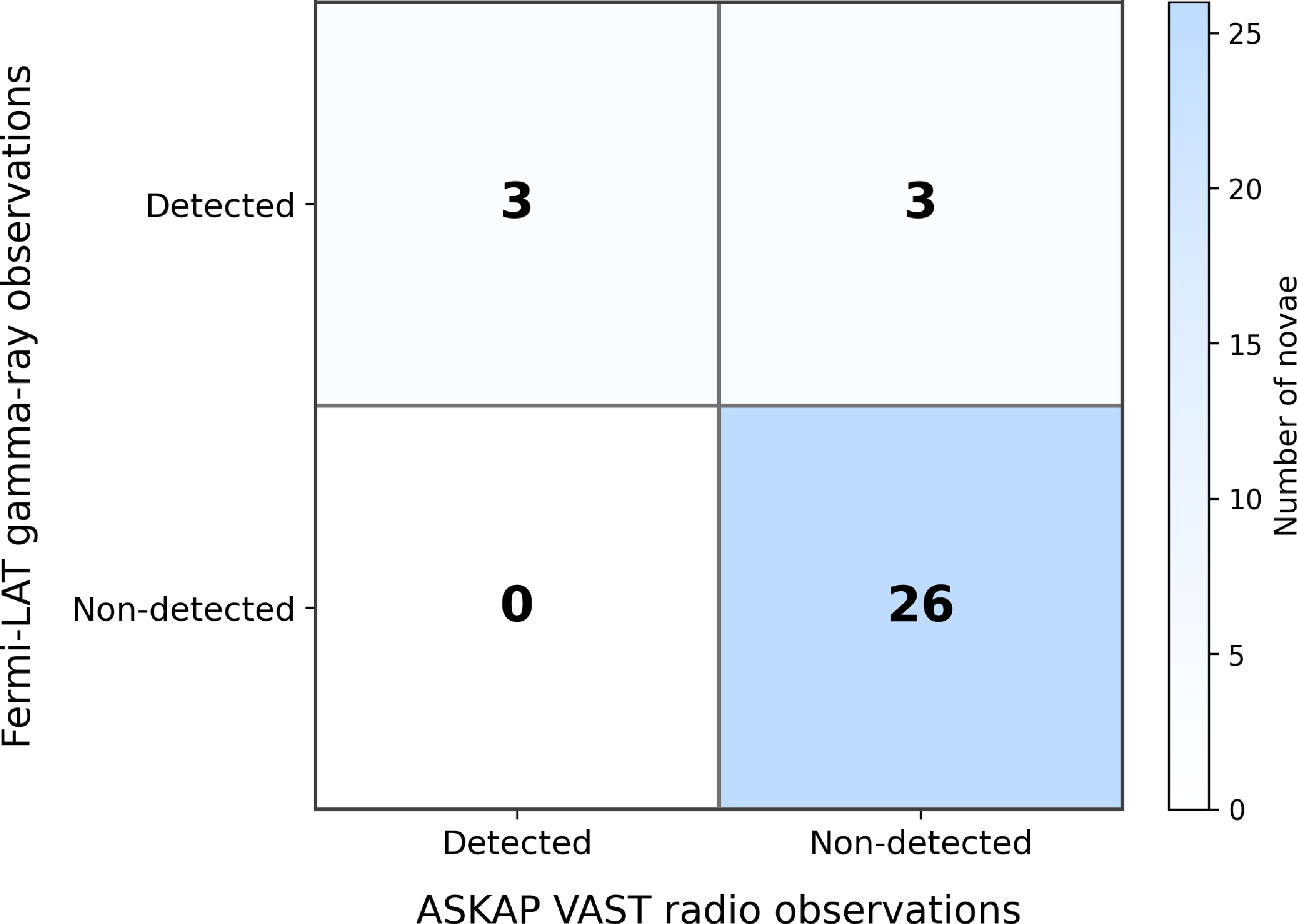
In Figure 10 we compare Fermi-LAT and ASKAP VAST detections to show that among the full ASKAP-footprint sample of 32 optically discovered classical novae from 2021 September to 2025 September, only six have reported gamma-ray emission. Notably, all three ASKAP VAST-detected novae in this work fall within this population. The radio detection fraction is 3/6 = 50%, with a 95% binomial confidence interval of approximately 12–88%. None of the 26 novae without Fermi-LAT detections were detected by ASKAP, corresponding to a radio detection fraction of 0/26 = 0% with a 95% upper confidence limit of approximately 13%. From this result, we estimated the p value as p ≃ 0.004 from the 2 × 2 contingency table in Figure 10, showing that the radio detection rate by ASKAP is significantly higher among gamma-ray-detected novae. The fact that ASKAP detected a subset that lies entirely within this LAT-detected population suggests that these radio observations may preferentially detect novae with strong shock activity or high intrinsic radio luminosities. This may suggest that gamma-ray emission is an early indicator of shock waves and particle acceleration processes, while later radio synchrotron emission reflects the same shock activity. From the observed radio evolution, we have seen that the timescale for the ejecta to become sufficiently transparent is approximately 100–150 days after the optical eruption. However, because only three of the six LAT-detected novae are detected by ASKAP, LAT detection is not sufficient to guarantee a radio detection. Sensitivity, cadence, distance, and intrinsic differences in the ejecta or circumbinary environment likely also affect whether a nova is detectable at 887.5 MHz.
This is the corner plot showing the posterior distributions from the broken power law synchrotron model fit with the lowest χ 2 value via MCMC analysis of V1723 Sco. Negative correlations in the energy-filling factor contour and a mildly positive correlation in the mass loss-wind velocity contour are observed; other than that, no significant correlations are spotted.

This shows how the radio evolution observed in classical novae can be affected by ejecta geometry, shock-wave properties, the density distribution of the circumstellar environment, and the emission mechanisms. It also highlights the limitations of simplistic models and the need for more complex, physically motivated models in subsequent studies.
6. Conclusion
In this paper, we fitted the radio light curves of three classical novae observed at 887.5 MHz with a two-week cadence. The model-fitting results can be summarised as follows:
-
• V6598 Sgr is best described by modified synchrotron emission rather than the other two emission models. It peaks at 5.3 ± 0.26 mJy and is consistent with a shock-driven non-thermal synchrotron source.
-
• V1716 Sco also exhibits an early non-thermal synchrotron flare. A broken power-law model provides a better fit than a single power-law model, indicating rapid evolution and efficient shock-driven particle acceleration.
-
• V1723 Sco is not well described by either model, though the broken power-law model captures the steep temporal evolution better than the single power-law model, suggesting an early non-thermal synchrotron flare with a much more complex ejecta structure.
Distribution of classical novae as a function of distance (kpc), separated by emission mechanisms. The histogram uses logarithmically spaced distance bins to provide equal-interval spacing. Most of the novae within 1 kpc show either non-detections or thermal radiation, while at large distances (≥ 4 kpc) the sample is dominated by the brighter, luminous non-thermal novae detectable in the ASKAP at 887.5 MHz.

Radio luminosity is plotted as observed at 887.5 MHz assuming the nominal distance for each source; the width of the shaded region denotes uncertainties on flux density.

Comparison of Fermi-LAT γ-ray and ASKAP VAST radio detections of novae, to assess whether radio detections are preferentially associated with prior gamma-ray detections. Each cell gives the number of novae in the corresponding detection category. The colour intensity scales with the number of sources per cell, with darker shading indicating a higher count. The estimated p ≃ 0.004 value from the binomial confidence interval shows that there is only about a 0.4% chance of getting a distribution like this, where all 3 ASKAP radio-detected novae fall within 6 Fermi-LAT gamma-ray-detected novae.

Gulati et al. (Reference Gulati2023) previously reported radio detections of four classical novae, where VAST data had limited temporal sampling, which they augmented with dedicated follow-up observations at higher frequencies. In contrast, our work here uses only the ASKAP VAST survey of regular, homogeneous monitoring at 887.5 MHz, enabling a well-sampled low-frequency light curve. This may then provide a template for the type of constraints that are feasible with future radio surveys, such as the Square kilometre Array (Dewdney et al. Reference Dewdney, Hall, Schilizzi and Lazio2009), where follow-up observations of large numbers of sources are not feasible.
This study highlights ASKAP’s role in identifying intrinsically bright classical novae at low radio frequencies. Especially when the typical thermal emission mechanism shapes the radio light curve and constrains the parameter, this early synchrotron flare at such a low frequency probes an unexplored regime in the nova evolutionary stage. We were able to model the light curves and analyse their rapid variability due to the dynamical evolution of the shock. This shows ASKAP’s capabilities to constrain shock energetics, ejecta-circumbinary material interactions, non-uniform ambient density, and a more complicatedly distributed emitting region. In the future, with multi-frequency observations and improved distance constraints, we will provide spectral evolution, a strong and direct diagnostic for identifying the emission mechanism. Therefore, we need unbiased continuous monitoring to obtain higher-quality data for more precise parameter estimation and to improve our understanding of the physics behind these star systems.
Acknowledgements
We thank an anonymous referee for helpful comments. This work was done as part of the ASKAP Variables and Slow Transients (VAST) collaboration (Murphy et al. Reference Murphy2013). DK was supported by NSF grant. AST-2511757. This research was supported by the Sydney Informatics Hub, a Core Research Facility of the University of Sydney. Parts of this research were supported by the Australian Research Council Centre of Excellence for Gravitational Wave Discovery (OzGrav), project number CE230100016. This scientific work uses data obtained from Inyarrimanha Ilgari Bundara, the CSIRO Murchison Radio-astronomy Observatory. We acknowledge the Wajarri Yamaji People as the Traditional Owners and native title holders of the Observatory site. CSIRO’s ASKAP radio telescope is part of the Australia Telescope National Facility (https://www.atnf.csiro.au/). Operation of ASKAP is funded by the Australian Government with support from the National Collaborative Research Infrastructure Strategy. ASKAP uses the resources of the Pawsey Supercomputing Research Centre. Establishment of ASKAP, Inyarrimanha Ilgari Bundara, the CSIRO Murchison Radio-astronomy Observatory, and the Pawsey Supercomputing Research Centre are initiatives of the Australian Government, with support from the Government of Western Australia and the Science and Industry Endowment Fund.

 M˙

 Vwind
 M˙
 Mej
 ϵ
 ϵ
 M˙

 M˙
 M˙
 ϵ
 ϵ
 M˙
 ρ∝M˙Vwind

 Open access

