



1. Introduction
The hydroelastic vibration analysis of complex elastic plates in full or partial contact with fluid is performed. The elastic deflection is two-dimensional, without any damping and external forcing. The elastic plate is thin, of finite length, with certain edge supports, with possible extra supports at some internal points of the plate, with cracks and other inhomogeneities. Both the thickness and rigidity of the plate may vary along the plate. The plate can be composed of different parts connected or not, but without gaps between the parts. The equilibrium shape of the plate is flat or can be well approximated as flat near the place of the plate contact with the fluid free surface. We shall determine eigenfrequencies and eigenmodes of such complex plates both in air and in contact with the fluid.
The fluid is inviscid and incompressible, of infinite depth and unbounded in horizontal directions. The fluid is at rest, with flat and horizontal free surface before the plate vibrations start. The interval of contact between the plate and the fluid free surface is given. Gravity, viscosity of the fluid and its surface tension are neglected, which is justified for frequencies of the plate vibration greater than  $\sqrt {g/L}$,
 $\nu /L^2$ and
 $\sqrt {\sigma /\rho L^3}$ correspondingly, where
 $g$ is the gravitational acceleration,
 $L$ is the characteristic length of the plate,
 $\nu$ is kinematic viscosity of the fluid,
 $\sigma$ is the surface tension coefficient and
 $\rho$ is the fluid density. Acoustic effects can be neglected for plate frequencies smaller than
 $c_0/L$, where
 $c_0$ is the sound speed in the fluid at rest. Gravity, surface tension and acoustic effects are responsible for decay of plate vibrations due to radiation of gravity, capillary and acoustic waves by the vibrating plate. Viscosity of the fluid and structural damping in the plate also lead to decay of plate vibrations in time. Therefore, natural or eigenvibrations of an elastic plate in air or in contact with a fluid could not exist without external forcing. However, the frequencies and shapes of such vibrations do not depend on forcing but on characteristics of the plate, fluid and the plate/fluid contact. Eigenfrequencies of a plate are the frequencies of excitation at which the plate resonates with the amplitudes of the plate responses being much higher than at other frequencies. In this way, the eigenfrequencies of dry plate vibrating in the air and wet plate vibrating in full or partial contact with a fluid can be measured. The corresponding shapes of the vibrations, which are known as eigenmodes of the plate, can be visualised with the Chladni figures, see Chladni (Reference Chladni1787). It was observed that the corresponding eigenmodes of a dry and wet elastic plate are close to each other but the corresponding eigenfrequencies of the wet plate are significantly smaller than those of the dry plate (see Korobkin Reference Korobkin1996b), where wet modes and frequencies of an elastic rectangular simply supported plate is contact with a liquid surface were computed and compared with the corresponding dry modes and frequencies.
Eigenfrequencies and modes of dry and wet plates are used to evaluate plate response and stresses in the plate caused by distributed external loads. Problems of an elastic plate in contact with a fluid free surface are especially challenging because deflections of the plate depend on the hydrodynamic loads which, in turn, depend on the plate deflections. Such problems are called coupled problems of hydroelasticity. They can be effectively solved using either dry modes of the plate and the so-called added-mass matrix of the modes or wet modes of the plate. If the wet modes are not used and the plate deflection in contact with the fluid is sought as a superposition of the dry modes with unknown in advance time-dependent coefficients, then this method is called the normal mode method. Within another approach, which cannot be used if the contact region between the plate and the fluid changes in time, the dry modes of an elastic complex plate are obtained first together with the corresponding frequencies. The wet modes are sought as superpositions of the dry modes with coefficients to be determined. The equation of thin plates and equations of hydrodynamics together with the boundary conditions provide an algebraic homogeneous system for the coefficients in the series of the wet modes. The eigen wet frequencies are obtained using the condition that the solutions of the algebraic system are non-zero. A superposition of the wet modes is then used to represent the plate deflection depending on the forcing.
Wet modes are solutions of a coupled linear hydroelastic problem. The flow caused by the plate vibration is described by a velocity potential, which satisfies Laplace's equation in the flow region and the linearised boundary conditions on the free surface and in the contact region between the fluid and the wetted surface of the elastic plate. The velocity potential in the contact region, which is needed for evaluating the hydrodynamic loads on the plate, is related to the time derivatives of the coefficients in the series for the plate deflection through an added-mass matrix. Once such a matrix is known, we can find the wet modes and their frequencies, as well as solve different problems of hydroelastic slamming including problems, where the size and position of the contact region vary in time.
To the best of the authors’ knowledge, added-mass matrices were introduced by Kvålsvold & Faltinsen (Reference Kvålsvold and Faltinsen1993, Reference Kvålsvold and Faltinsen1995) in the problem of wave impact onto a wetdeck of a multihull vessel. The wetdeck was modelled as Euler and Timoshenko beams correspondingly. Hydrodynamics loads were evaluated within the Wagner theory of water impact. It seems that the concept of added-mass matrices was not used in numerical computations before the papers by Kvålsvold & Faltinsen (Reference Kvålsvold and Faltinsen1995) and Faltinsen (Reference Faltinsen1997). Elements of the added-mass matrix were given by integrals and by series of Bessel functions in these two papers correspondingly. The plate deflection in the impact region was approximated by a linear function in Kvålsvold & Faltinsen (Reference Kvålsvold and Faltinsen1995) and by a Fourier series in Faltinsen (Reference Faltinsen1997). Inspired by work of Faltinsen and his group, Korobkin (Reference Korobkin1995) used the same approach in the problem of wave impact on the bow end of a catamaran wetdeck. He showed that the elements of the corresponding added-mass matrix are given by double singular integrals, which were evaluated numerically. The contact region between an elastic wetdeck and impacting wave was expanding in time. The added-mass matrix had to be computed at each time step of integration of the elastic plate equation in time. This made calculations of the wetdeck response using the concept of added-mass matrix impractical. Korobkin (Reference Korobkin1995) performed numerical calculations only within the one-mode approximation.
Added-mass matrix was obtained in analytical form by Khabakhpasheva & Korobkin (Reference Khabakhpasheva and Korobkin1997) for an elastic plate, edges of which are supported by springs; however, details of analytical calculations were not given. The formulae for the elements of the added-mass matrices of a simply supported Euler plate impacted by a wave were published by Korobkin (Reference Korobkin1998) for symmetric impact and by Korobkin & Khabakhpasheva (Reference Korobkin and Khabakhpasheva1998) for asymmetric impact. Only Bessel functions  $J_0(x)$ and
 $J_1(x)$ appeared in the formulae. These analytical formulae made it possible to perform calculations of wave impact on elastic plates with large number of modes demonstrating convergence of the numerical solution for the elastic stresses. The obtained added-mass matrices were used by Korobkin & Khabakhpasheva (Reference Korobkin and Khabakhpasheva1999a) to find the modes of an elastic plate vibration in full contact with the fluid free surface, which are the so-called wet modes. It was shown that the lowest dry and wet modes are close to each other, see also Faltinsen, Kvålsvold & Aarsnes (Reference Faltinsen, Kvålsvold and Aarsnes1997).
Added-mass matrix for a cylindrical shell entering water was calculated by Ionina & Korobkin (Reference Ionina and Korobkin1999) and Ionina (Reference Ionina1999). Reinhard, Korobkin & Cooker (Reference Reinhard, Korobkin and Cooker2013) and Reinhard (Reference Reinhard2013) calculated the added-mass matrix for water impact of an elastic plate at high horizontal speed.
In three-dimensional impact problems, added-mass matrices were derived for circular elastic plates by Scolan (Reference Scolan2004), Pegg, Purvis & Korobkin (Reference Pegg, Purvis and Korobkin2018), and Vega-Martinez et al. (Reference Vega-Martinez, Rodriguez-Rodriguez, Khabakhpasheva and Korobkin2019) to investigate different problems of water impact and water exit. Three-dimensional problems are not considered in this paper.
Added-mass matrices of floating elastic plates were used by Khabakhpasheva & Korobkin (Reference Khabakhpasheva and Korobkin2021) to study stresses in the plates caused by a rigid body impact onto the plates.
The papers cited above deal with homogeneous plates of constant thickness with different edge conditions. However, it was shown that the normal mode method and the concept of added-mass matrix can be used for complex structures as well. Khabakhpasheva & Korobkin (Reference Khabakhpasheva and Korobkin2003, Reference Khabakhpasheva and Korobkin2013) applied this method to the problem of an elastic wedge entering water and studied different approximations of the corresponding added-mass matrix. Fu & Qin (Reference Fu and Qin2014) used the discrete vortex method to calculate the added-mass matrix for elastic wedges. It was shown that the elements of the added-mass matrix computed numerically well approximate the elements evaluated by Khabakhpasheva & Korobkin (Reference Khabakhpasheva and Korobkin2013). Feng et al. (Reference Feng, Zhang, Wan, Jiang, Sun and Zong2021) obtained an added-mass matrix by boundary element method and used it to solve numerically coupled problems of hydroelastic slamming. Korobkin, Gueret & Malenica (Reference Korobkin, Gueret and Malenica2006) calculated the added-mass matrix for finite-element model of an elastic wedge.
The experience gained with calculations of the added-mass matrixes in problems of hydroelastic slamming is generalised in the present paper to complex elastic structures made of several different sections with different types of connectors between them. It is impossible to cover all configurations. The algorithm of obtaining added-mass matrices is described in the following in several steps.
The problem of a free–free floating plate of constant thickness is formulated in § 2 in dimensionless variables. The wet modes, their frequencies, and the corresponding added-mass matrix are introduced. The added-mass matrix of such a plate is obtained in § 3. The algorithm is explained in full details. In § 4, the results of § 3 are generalised to different edge conditions (§ 4.1) and partly wetted plates (§ 4.2). Added-mass matrix and wetted modes of a complex floating structure made of several plates of constant thicknesses with internal supports and connectors are studied in § 5. Plates of variable thickness are considered in § 6. It is shown in § 6.2 how to calculate the added-mass matrix and wetted modes for a plate with a piecewise linear thickness. The algorithm is illustrated by examples for particular compositions of floating structures. Relations between dry and wet modes and dry and wet frequencies are investigated for each example. The numerical algorithm of the present paper and the obtained results are summarised in § 7. The paper cannot be considered as a handbook/catalogue of solutions of hydroelastic problems. Sections of the paper are intended to guide readers and help them to derive wet modes and added-mass matrices for their own practical problems.
2. Formulation of the wet mode problem
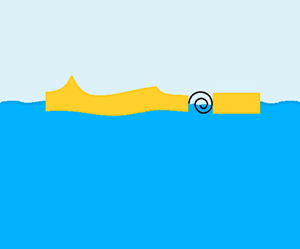
A free–free elastic plate of contact thickness  $h$ is placed on the surface of inviscid and incompressible fluid of infinite depth. The edges of the plate are free of stresses and shear forces. The plate length
 $2L$ is much greater than the plate thickness. At equilibrium the fluid free surface is flat and horizontal. The plate floats on the fluid surface with its draft being smaller than the plate thickness
 $h$. The flow and plate deflection are described in the Cartesian coordinate system
 $Ox'y'$, see figure 1. The line
 $y'=0$ corresponds to the equilibrium position of the fluid free surface. A prime stands for dimensional variables. The origin of the system is at the plate centre. The plate position can be approximated in the leading order by the interval
 $y'=0$,
 $-L< x'< L$. The plate deflection,
 $y'=w'(x',t')$, is described by the Euler beam equation, see Timoshenko & Young (Reference Timoshenko and Young1955),
 \begin{equation} m\frac{\partial^2w'}{\partial t'^2} +D \frac{\partial^4w'}{\partial x'^4}=p'(x',0,t')\quad ({-}L< x'< L) \end{equation}
with the edge conditions
 \begin{equation} \frac{\partial^2w'}{\partial x'^2}=0,\quad \frac{\partial^3w'}{\partial x'^3}=0 \quad(x'={\pm} L), \end{equation}
where  $m$ is the mass of the plate per unit area,
 $D$ is the rigidity coefficient and
 $p'(x',0,t')$ is the hydrodynamic pressure acting on the wetted surface of the plate. Within the linear theory of hydroelasticity, the hydrodynamic pressure is given by the linearised Bernoulli equation,
 $p'(x',y',t')=-\rho \partial \varphi '/\partial t$, where
 $\rho$ is the fluid density and
 $\varphi '(x',y',t')$ is the velocity potential which is the solution of the following boundary-value problem
 $$\begin{gather} \nabla^2\varphi'=0\quad (y'<0), \end{gather}$$
 $$\begin{gather}\varphi'(x',0,t')=0\quad (y'=0,\ |x'|>L), \end{gather}$$
 $$\begin{gather}\frac {\partial \varphi'}{\partial y'}(x',0,t')= \frac {\partial w'}{\partial t'}(x',t') \quad (y'=0,\ |x'|< L), \end{gather}$$
 $$\begin{gather}\varphi'\to 0 \quad(x'^2+y'^2\to\infty). \end{gather}$$
The boundary condition on the plate, where  $y'=0$ and
 $|x'|< L$, is linearised and imposed on the equilibrium level of the fluid without account for the plate draft and deflection in the leading order for a thin plate, small draft and small plate deflection. The dynamic boundary condition on the free surface, where
 $y'=0$ and
 $|x'|>L$, is also linearised. Note that gravity effects are not included in (2.1)–(2.3). The velocity potential satisfies Laplace's equation in the flow region,
 $y'<0$, and decays with distance from the plate. Initial conditions are not required.
Floating elastic plate and notation.

The flow velocity given by the gradient  $\boldsymbol {\nabla } \varphi '$ is unbounded at the edges of the plate,
 $x'=\pm L$,
 $y'=0$, see Faltinsen et al. (Reference Faltinsen, Kvålsvold and Aarsnes1997), Gakhov (Reference Gakhov2014) and Korobkin (Reference Korobkin1996a). The vertical velocity component on the free surface, where
 $y'=0$ and
 $|x'|>L$, behaves as
 $\partial \varphi '/\partial y'(x',0,t')=O([(x')^2-L^2]^{-1/2})$ near the plate edges. Correspondingly, the horizontal velocity component on the plate,
 $y'=0$,
 $|x'|< L$, behaves as
 $\partial \varphi '/\partial x'(x',0,t')=O([L^2-(x')^2]^{-1/2})$ at the edges. The velocity potential is continuous at the edges and behaves there as
 $\varphi '(x',0,t')=O([L^2-(x')^2]^{1/2})$. Only the velocity potential will be required in the following in calculations of the wet modes and their frequencies, as well as in calculations of the elements of the added-mass matrix. The distribution of the velocity potential along the plate is given by a Cauchy principal value integral, see Appendix A.
We shall determine time-periodic solutions of the coupled problem (2.1)–(2.3) and the corresponding frequencies  $\omega$,
 \begin{equation} w'(x',t')=W'(x')\cos(\omega t'),\quad \varphi(x',y',t')={-}\varPhi'(x',y')\sin(\omega t'). \end{equation}
There is no forcing in this formulation.
Dimensionless variables, which are denoted by the same symbols without primes,
 \begin{equation} x'=Lx, \quad y'=Ly, \quad t'=t/\omega,\quad W'=W_{sc}W(x), \quad \varPhi'=\omega W_{sc} L\,\varPhi(x,y), \end{equation}
are used in the following. Here  $W_{sc}$ is a formal scale of deflection. Equations (2.1)–(2.4) provide the following coupled problem for the shapes of the eigenoscillations of the floating plate
 $W(x)$ and the corresponding potential
 $\varPhi (x,y)$ in the dimensionless variables (2.5),
 $$\begin{gather} \frac{{\rm d}^4W}{{\rm d}\kern0.7pt x^4}=\varOmega [\alpha W+\varPhi(x,0)]\quad (|x|<1),\quad \frac{{\rm d}^2W}{{\rm d}\kern0.7pt x^2}=\frac{{\rm d}^3W}{{\rm d}\kern0.7pt x^3}=0\quad (x={\pm} 1), \end{gather}$$
 $$\begin{gather}\nabla^2\varPhi=0\quad (y<0), \end{gather}$$
 $$\begin{gather}\varPhi=0\quad(y=0,\ |x|>1),\quad \varPhi_y=W(x) \quad (y=0,\;|x|<1), \end{gather}$$
where  $\alpha =m/\rho L$,
 $\varOmega =\rho L^5 \omega ^2/D$. There are two ‘static’ non-zero solutions of the eigenvalue problem (2.6)–(2.8),
 $W_1(x)=C_1$ and
 $W_2(x)=C_2 x$, where
 $C_1$ and
 $C_2$ are any constants, corresponding to eigenvalues
 $\varOmega _1=\varOmega _2=0$. Other solutions
 $W_k(x)$ correspond to
 $\varOmega _k>0$. The solutions
 $W_k(x)$ are called wet rigid (
 $k=1,2$) and elastic (
 $k\ge 3$) modes of the floating plate in the dimensionless variables. These modes are not normalised and they are not orthogonal in a standard sense. The dimensional frequencies of the wet elastic modes are given by
 $\omega _k=[\varOmega _k D/(\rho L^5)]^{1/2}$.
The non-zero solutions of the boundary problem (2.6) with  $\varPhi (x,0)=0$ are known as the dry modes
 $\psi _n(x)$. The dry modes are the solutions of the spectral problem,
 \begin{equation} \frac{{\rm d} ^4\psi_n}{{\rm d}\kern0.7pt x^4}=\lambda_n^4 \psi_n\quad (|x|<1),\quad \frac{{\rm d} ^2\psi_n}{{\rm d}\kern0.7pt x^2}=\frac{{\rm d} ^3\psi_n}{{\rm d}\kern0.7pt x^3}=0\quad (x={\pm} 1), \end{equation}
where  $\lambda _n$ is a spectral parameter,
 $n\ge 1$. The dry modes
 $\psi _n(x)$ are orthogonal and normalised,
 \begin{equation} \int_{{-}1}^1 \psi_n(x)\psi_m(x) \,{\rm d}\kern0.7pt x=\delta_{nm}, \end{equation}
where  $\delta _{nn}=1$ and
 $\delta _{nm}=0$ for
 $n\ne m$. There are two modes,
 $\psi _1(x)=1/\sqrt {2}$ and
 $\psi _2(x)=\sqrt {3/2}x$, which satisfy (2.9) and correspond to
 $\lambda _1=\lambda _2=0$. There are the rigid modes of the free–free plate. Elastic dry modes start from
 $n=3$. Dry dimensionless modes of Euler beam,
 $\psi _n(x)$, and the corresponding eigenvalues
 $\lambda _n$ are independent of elastic characteristics of the beam but on the edge conditions only. The frequencies of the elastic dry modes are
 $\omega _n^{(d)}=\lambda _n^2[D/(m L^4)]^{{1}/{2}}$.
The wet elastic modes  $W_k(x)$,
 $k\ge 3$, are sought as superpositions of the dry modes,
 \begin{equation} W_k(x)=\sum_{n=1}^\infty W_{kn}\psi_n(x), \end{equation}
with coefficients  $W_{kn}$ and the eigenvalues
 $\varOmega _k$ to be determined. Note that the rigid dry modes,
 $\psi _1(x)$ and
 $\psi _2(x)$, also contribute to the wet elastic modes.
The corresponding velocity potential  $\varPhi _k(x,y)$ can be decomposed as
 \begin{equation} \varPhi_k(x,y)=\sum_{n=1}^\infty W_{kn} \phi_n(x,y), \end{equation}
by using series (2.11) and the boundary condition on the plate, where  $y=0$ and
 $x\le 1$. The new potentials
 $\phi _n(x,y)$ are solutions of the following problems
 \begin{gather} \nabla^2\phi_n=0 \quad (y<0), \end{gather}
 \begin{gather} \phi_n=0 \quad (y=0,\ |x|>1),\quad \frac{\partial \phi_n}{\partial y}=\psi_n(x)\quad (y=0,\ |x|<1). \end{gather}
Substituting the series (2.11) and (2.12) in (2.6), multiplying the result by  $\psi _m(x)$,
 $m\ge 1$, and integrating both sides of the equation with respect to
 $x$ from
 $-1$ to
 $+1$, we arrive at the matrix equation
 \begin{equation} [\boldsymbol{\mathsf{D}}-\varOmega_k (\alpha \boldsymbol{\mathsf{I}}+\boldsymbol{\mathsf{S}})]\boldsymbol{W_k} =0 \end{equation}
for the vector  $\boldsymbol {W_k}=(W_{k1}, W_{k2}, W_{k3},\ldots )^{\rm T}$ of the coefficients in the series (2.12). Here
 $\boldsymbol{\mathsf{D}}$ is diagonal matrix,
 $D_{nm}=0$ for
 $n\ne m$,
 $D_{nn}=\lambda ^4_n$,
 $\boldsymbol{\mathsf{I}}$ is the unit matrix,
 $I_{nm}=\delta _{nm}$, and
 $\boldsymbol{\mathsf{S}}$ is the so-called added-mass matrix,
 \begin{equation} S_{nm}=\int_{{-}1}^1 \phi_n(x,0)\psi_m(x)\,{\rm d}\kern0.7pt x. \end{equation}
The added-mass matrix is symmetric,  $S_{nm}=S_{mn}$, which follows from Green's second identity. Therefore, the matrix of (2.15) is symmetric, as a sum of symmetric matrices, and the eigenvalues
 $\varOmega _k$ of this matrix equation are real and positive. The eigenvalues
 $\varOmega _k$ are the solutions of the equation
 \begin{equation} \det [\boldsymbol{\mathsf{D}}-\varOmega_k (\alpha \boldsymbol{\mathsf{I}}+\boldsymbol{\mathsf{S}})] =0. \end{equation}
The vector  $\boldsymbol {W_k}$ is the eigenvector of the matrix
 $[\boldsymbol{\mathsf{D}}-\varOmega _k (\alpha \boldsymbol{\mathsf{I}}+\boldsymbol{\mathsf{S}})]$.
Equation (2.17) for the eigenvalues  $\varOmega _k$ and the infinite system of the algebraic (2.15) for the coefficients
 $W_{nk}$ are solved by truncation retaining
 $N_w$ equations in (2.15) and setting
 $W_{kn}=0$ for
 $n>N_{mod}$. Practical convergence of the numerical solution is achieved by increasing the number
 $N_{mod}$. The numerical calculations are straightforward if the added-mass matrix
 $\boldsymbol{\mathsf{S}}$ is known for a large number of its elements.
The wet modes  $W_k(x)$ given by (2.11) satisfy the edge conditions at
 $x=\pm 1$ because the dry modes
 $\psi _n(x)$ satisfy these conditions, see (2.6), (2.9) and (2.11). The wet modes are orthogonal in the following sense,
 \begin{equation} \int_{{-}1}^1(\alpha W_nW_m+\varPhi_n(x,0)W_m(x))\,{\rm d}\kern0.7pt x=0\quad(n\ne m). \end{equation}
The prove (2.18), one should write (2.6) for  $W_n(x)$ and
 $\varOmega _n$, multiply both sides by
 $W_m(x)$,
 $m\ne n$, and integrate the results in
 $x$ from
 $-1$ to
 $+1$. The left-hand side of the resulting equation is integrated by parts twice using the edge conditions. Then we swap
 $n$ and
 $m$ and subtract the new equation from the original one. Finally using Green's second identity for
 $\varPhi _n$ and
 $\varPhi _m$ and the fact that
 $\varOmega _n\ne \varOmega _m$ for
 $n\ne m$, we arrive at (2.18). The orthogonality relation (2.18) can be used to solve problems of impact onto a floating ice plate, see Khabakhpasheva & Korobkin (Reference Khabakhpasheva and Korobkin2021).
3. Added mass matrix of free–free floating plate
It was shown in § 2 that the wet modes of a floating elastic plate and the corresponding frequencies can be accurately calculated if the added-mass matrix  $S$ given by (2.16) is known for large number of its elements. It will be shown in full details in this section for a free–free floating elastic plate how to evaluate integrals (2.16) analytically through the Bessel functions. In the following sections, it will be shown how to modify the analysis of this section to evaluate added-mass matrices for different edge conditions, partly wetted plates, cracked plates, plates with variable thickness, as well as how to apply the added-mass matrices to different problems of hydroelastic slamming.
3.1. Dry modes of free–free elastic plate
The added-mass matrix (2.16) describes interactions of the dry modes  $\psi _n(x)$ through the fluid, see (2.9) and (2.14). A general solution of the fourth-order differential equation (2.9) has the form
 $$\begin{gather} \psi_n(x)=L_{n1}f_{n1}(x)+L_{n2}f_{n2}(x)+L_{n3}f_{n3}(x)+L_{n4}f_{n4}(x), \end{gather}$$
 $$\begin{gather}f_{n1}(x)=\cos (\lambda_n x),\quad f_{n2}(x)=\sin(\lambda_n x),\quad f_{n3}(x)={\rm e}^{-\lambda_n(1+x)},\quad f_{n4}={\rm e}^{-\lambda_n (1- x)}, \end{gather}$$
where  $L_{nj}$,
 $j=1, 2, 3, 4$, are coefficients specific for imposed edge conditions. Substituting (3.1) in the four edge conditions we arrive at four equations with respect to the coefficients
 $L_{nj}$. The right-hand sides of these linear equations are zero. Non-zero solutions of the system exist only for some special values of the spectral parameter
 $\lambda _n$, which are obtained by equating the determinant of the system to zero. These solutions are determined up to factors, which are obtained using the normalisation condition (2.10). For a free–free dry plate with the edge conditions shown in (2.9), we obtain two modes,
 $n=1$ and
 $n=2$, with
 $\lambda _1=\lambda _2=0$, which correspond to rigid motions of the plate,
 \begin{equation} \psi_1(x)=\frac 1{\sqrt 2},\quad \psi_2(x)=\sqrt{\frac 32} x, \end{equation}
and normalised elastic modes (3.1), where
 \begin{equation} L_{n1}=\frac{1}{\sqrt{2}\cos\lambda_n},\quad L_{n2}=0,\quad L_{n3}=\frac{1}{\sqrt{2}(1+{\rm e}^{{-}2\lambda_n})},\quad L_{n4}=L_{n3}, \end{equation}
for odd numbers,  $n=2m+1$,
 $m\geq 1$, and
 \begin{equation} L_{n1}=0,\quad L_{n2}=\frac{1}{\sqrt{2}\sin\lambda_n},\quad L_{n3}=\frac{-1}{\sqrt{2}(1-{\rm e}^{{-}2\lambda_n})},\quad L_{n4}={-}L_{n3}, \end{equation}
for even numbers,  $n=2m+2$,
 $m\geq 1$. Here
 $\lambda _n$ are real positive roots of the equation,
 \begin{equation} \cosh(2\lambda_n) \cos(2\lambda_n)=1. \end{equation}
For large  $n$ we have
 \begin{equation} \lambda_n=\frac{\rm \pi}{4}(n-2)+O({\rm e}^{-({\rm \pi}/{2})n}),\quad |L_{n3}|=\frac 1{\sqrt 2}+O({\rm e}^{-({\rm \pi}/{2})n}), \end{equation}
see, for example, Khabakhpasheva & Korobkin (Reference Khabakhpasheva and Korobkin2021).
3.2. Added masses as bilinear forms of dry modes
The elements  $S_{nm}$ of the added-mass matrix, where
 $n,m\geq 1$, are given by the integral (2.16) and depend on the mode
 $\psi _m(x)$ directly and on the mode
 $\psi _n(x)$ through the potential (2.14) in the interval
 $y=0$,
 $-1< x<1$. It is convenient to introduce a bilinear form
 \begin{equation} U[F(x),G(x)]=\int_{{-}1}^1 \varPsi(x,0)G(x)\,{\rm d}\kern0.7pt x, \end{equation}
where  $F(x)$ and
 $G(x)$ are smooth functions defined in the interval
 $-1< x<1$, and the potential
 $\varPsi (x,y)$ is the solution of the following mixed boundary-value problem,
 \begin{equation} \nabla^2 \varPsi=0\ \ (y<0),\quad\varPsi=0 \ \ (y=0,\ |x|>1),\quad\varPsi_y=F(x)\ \ (y=0, |x|<1), \end{equation}
which decays at infinity,  $\varPsi \to 0$ as
 $x^2+y^2\to \infty$, and is continuous in
 $y\leq 0$. The bilinear form
 $U[F(x),G(x)]$ has the following properties:
(a) it is symmetric,
(3.10)which follows from Green's second identity; \begin{equation} U[F(x),G(x)] = U[G(x),F(x)], \end{equation}
(b) it is linear with respect to each argument,
(3.11)$$\begin{gather} U[C_1F_1(x)+C_2F_2(x),G(x)]=C_1 U[F_1(x),G(x)]+ C_2U[F_2(x),G(x)], \end{gather}$$(3.12)$$\begin{gather}U[F(x),C_1G_1(x)+C_2G_2(x)]=C_1 U[F(x),G_1(x)]+ C_2U[F(x),G_2(x)]; \end{gather}$$(c) it is zero if the product
$F(x)G(x)$ is an odd function of $x$;(d)
(3.13)where plus is for even\begin{equation} U[F({-}x),G(x)]=U[F(x),G({-}x)]={\pm} U[F(x),G(x)], \end{equation}$G(x)$ and minus is for odd $G(x)$;(e)
(3.14)where\begin{equation} U[{\rm e}^{\alpha x},{\rm e}^{\beta x}]=\begin{cases} {\rm \pi}[ I_0(\alpha)I_1(\beta)+I_1(\alpha)I_0(\beta)]/(\alpha+\beta)\quad (\alpha\neq{-}\beta), \\ {\rm \pi}[ I^2_0(\alpha)-I^2_1(\alpha)-I_0(\alpha)I_1(\alpha)/\alpha]\quad (\alpha={-}\beta), \end{cases} \end{equation}$\alpha$ and $\beta$ are complex numbers and $I_0(\alpha )$, $I_1(\alpha )$ are the modified Bessel functions of the first kind; formula (3.14) is derived in Appendix A.


Then  $S_{nk}=U[\psi _k(x),\psi _n(x)]$, where
 $\psi _n(x)$ is given by (3.4) for
 $n\geq 3$ and by (3.3) for
 $n=1$ and
 $n=2$. Let us consider first the elastic modes,
 $n, k\geq 3$, and the corresponding elements of the added-mass matrix. Substituting (3.1) in the bilinear form, we find
 \begin{equation} S_{nk}=U[\psi_k(x),\psi_n(x)]=\sum_{j=1}^4 \sum_{i=1}^4 L_{kj} U[f_{kj}(x),f_{ni}(x)] L_{ni} =\boldsymbol{L}_{\boldsymbol{k}}\boldsymbol{\cdot}\boldsymbol{\mathsf{Se}}^{(\boldsymbol{\mathsf{nk}})}\boldsymbol{\cdot} \boldsymbol{L}_{\boldsymbol{n}},\end{equation}
where  $\boldsymbol {L}_{\boldsymbol {n}}=(L_{n1},L_{n2},L_{n3},L_{n4})$ and
 $\boldsymbol{\mathsf{Se}}^{(\boldsymbol{\mathsf{nk}})}$ is a symmetric
 $4\times 4$ matrix with the elements
 \begin{equation} Se^{(nk)}_{ij} =U[f_{kj}(x),f_{ni}(x)]\quad (1\leq i,j\leq4,\ n, k\geq 3). \end{equation}
Note that  $Se^{(nk)}_{12}=Se^{(nk)}_{21}=0$, which follows from (3.2) and property (d) of the bilinear form (3.13). As a result, calculations of the elastic part of the added-mass matrix are reduced to evaluation of eight integrals (3.16). Other elements of the matrix are obtained using the symmetry relation
 $Se^{(nk)}_{ij}=Se^{(kn)}_{ji}$. The elements
 $Se^{(nk)}_{ij}$ are evaluated using properties of the bilinear form and (3.2) and (3.14). For example,
 \begin{align} Se^{(nk)}_{34}&= U[{\rm e}^{-\lambda_k(1+x)},{\rm e}^{-\lambda_n(1-x)}]={\rm e}^{-\lambda_k-\lambda_n}U[{\rm e}^{-\lambda_kx},{\rm e}^{\lambda_nx}]\nonumber\\ & = \begin{cases} {\rm \pi}[\tilde{I}_1(\lambda_n)\tilde{I}_0(\lambda_k)- \tilde{I}_1(\lambda_k)\tilde{I}_0(\lambda_n)]/(\lambda_n-\lambda_k)\quad (n\neq k),\\ {\rm \pi}[\tilde{I}^2_0(\lambda_n)-\tilde{I}_1^2(\lambda_n)-\tilde{I}_0(\lambda_n)\tilde{I}_1(\lambda_n)/\lambda_n] \quad(n=k), \end{cases} \end{align}
where  $\tilde {I}_0(x)=I_0(x) \,{\rm e}^{-x}$ and
 $\tilde {I}_1(x)=I_1(x) \,{\rm e}^{-x}$ for
 $x\geq 0$. We used in (3.17) that
 $I_0(x)$ is even and
 $I_1(x)$ is odd functions. Other elements for both elastic and rigid modes are calculated analytically in Appendix A.
3.3. Wet modes of free–free plate and their frequencies
The elastic  $k$th wet mode,
 $k\geq 3$, is given by series (2.11), where the coefficients
 $W_{kn}$ are solutions of the algebraic system (2.15). The value
 $\varOmega _k$ is a solution of the (2.17). This solution depends on a single parameter
 $\alpha$. The solutions are real because the matrix of the system (2.15) is symmetric but not necessary positive. Only positive solutions of (2.17) provide the frequencies of the wet modes,
 $\omega _k=[\varOmega _k D/(\rho L^5)]^{1/2}$. We consider only positive solutions. We truncate the matrix
 $[\boldsymbol{\mathsf{D}}-\varOmega (\alpha \boldsymbol{\mathsf{I}}+\boldsymbol{\mathsf{S}})]$ retaining
 $N_{mod}$ terms and calculate its determinant as a function of
 $\varOmega$ with a certain step in
 $\varOmega$ starting from
 $\varOmega =0$. The intervals, where the determinant changes its sign, are identified and the bisection method is used within each interval to find the roots
 $\varOmega _k$,
 $1\leq k\leq N_{mod}$, with required accuracy of
 $10^{-4}$. Then the roots are determined for larger number of retained terms
 $N_{mod}$ to confirm convergence of the roots with respect to the number of retained equations. The system (2.15) is solved for each root
 $\varOmega _k$, convergence of which has been confirmed.
The only parameter of the problem,  $\alpha$, is small in the theory of thin plates. The ratios of wet,
 $\omega _n$, and dry,
 $\omega _n^{(d)}$, elastic natural frequencies,
 \begin{equation} \frac{\omega_n}{\omega^{(d)}_n}=\frac {\sqrt{\alpha\varOmega_n}}{\lambda_n^2}, \quad \omega_n=\left(\frac{\varOmega_n D}{\rho L^5}\right)^{1/2}, \quad \omega_n^{(d)}=\lambda_n^2 \left(\frac{D}{m L^4}\right)^{{1}/{2}}, \end{equation}
are shown in figure 2(a) for different numbers  $n\geq 3$ and different
 $\alpha$. Note that this ratio is independent of the plate rigidity. The ratios are not monotonic for
 $n=3,4,5$, then monotonically increase with increase of
 $n$ for all values of
 $\alpha$, and approach 1 for large
 $n$. The ratios increase with increase of
 $\alpha$ for any
 $n$, and are always smaller than one. Wet frequencies are also defined for
 $\alpha =0$, where the ratios tend to zero. Scaled wet frequencies for small α are shown in figure 2(b). To confirm convergence of the results, calculations for
 $\alpha =0.1$ and
 $0.01$ were performed with
 $N_{mod}$ equal to 30 and 50. It was found that the absolute differences of the ratios
 $\omega _n/\omega _n^{(d)}$ calculated with
 $N_{mod}=30$ and
 $N_{mod}=50$ for
 $3\leq n\leq 20$ is less that
 $5\times 10^{-6}$ for both values of
 $\alpha$.
The ratio (3.18a–c) of the wet and dry frequencies (a) and the scaled ratios for small  $\alpha$ (b) as functions of the frequency number for different values of the parameter
 $\alpha$.

For each root  $\varOmega _k$, we set
 $W_{kk}=1$ in (2.15), truncate the system to
 $N_{mod}$ equations and
 $N_{mod}$ unknowns, move
 $k$th column of (2.15) to the right-hand side and cut
 $k$th row from the system. The obtained finite system with non-zero right-hand side is solved numerically. The elements
 $W_{kn}$ of the resulting vector
 $\boldsymbol {W}_{\boldsymbol {k}}$ are listed in table 1 for
 $\alpha =0.01$ with three significant figures. Red entries in this table are for
 $W_{kk}$ which are set to one. It is seen that the wet modes have approximately the same shapes as the corresponding dry modes, but the natural frequencies of the modes are very different, see figure 2. The main contribution to the
 $k$th wet mode comes from the
 $k$th dry mode, the second mode, which provides the highest contribution, is the
 $(k+1)$th mode but its contribution is less than
 $10\,\%$ for even modes and
 $20\,\%$ for odd modes.
The coefficients  $W_{kn}$ in the series (2.11) of the
 $k$th wet mode as superposition of the dry modes
 $\psi _n(x)$ for
 $\alpha =0.01$. Wet modes with odd numbers are listed in the top of the table and the wet modes with even numbers are listed in the bottom of the table.

4. Partially wetted elastic plate with different edge conditions
In this section, the results from § 3 are generalised to other edge conditions and to elastic plates, only part of which is in contact with a fluid.
4.1. Added-mass matrix of elastic plate with different edge conditions
For edge conditions different from those in (2.6), eigenmodes of an elastic dry plate still have the form (3.1), (3.2) but with the coefficients  $L_{nj}$ and
 $\lambda _n$ being specific for these conditions. The elements of the added-mass matrix are still given by (3.15) with the
 $4\times 4$ matrix
 $\boldsymbol{\mathsf{Se}}^{(\boldsymbol{\mathsf{nk}})}$ being independent of the edge conditions. For example, for a simply supported plate in full contact with the fluid, the edge conditions in (2.6) should be changed for
 $W(\pm 1)=W''(\pm 1)=0$, which provide the following end conditions in the spectral problem (2.9),
 $\psi _n=\psi ''_n=0$ at
 $x=\pm 1$. Symmetric dry modes of such a plate and the corresponding eigenvalues read
 \begin{equation} \psi_n(x)=\cos(\lambda_n x), \quad \lambda_n={-}\frac{\rm \pi}{2}+{\rm \pi} n \quad (n\geq 1). \end{equation}
Therefore,  $L_{n1}=1$ and
 $L_{n2}=L_{n3}=L_{n4}=0$ in (3.1) and the elements of the added-mass matrix (3.15) for symmetric vibrations of the plate are given by (see Appendix A)
 \begin{align} S_{nk}&=U[\cos(\lambda_k x), \cos(\lambda_n x)]=Se^{(nk)}_{11}\nonumber\\ &=\begin{cases} {\rm \pi}[ \lambda_n J_1(\lambda_n)J_0(\lambda_k) -\lambda_k J_1(\lambda_k)J_0(\lambda_n)]/(\lambda_n^2 - \lambda_k^2)\quad (n\neq k), \\ {\rm \pi}[ J^2_0(\lambda_n)+J^2_1(\lambda_n)]/2 \quad (n=k). \end{cases} \end{align}
The added-mass matrix (4.2) corresponds to that in Korobkin (Reference Korobkin1998, equation (41)) with  $c=1$, where the plate is completely wetted.
4.2. Added-mass matrix of an elastic plate in partial contact with fluid
An elastic plate corresponds to the interval  $-1< x<1$ in the dimensionless variables (2.5). However, now only a part of the plate,
 $a< x< b$, is in contact with the fluid, where
 $-1\leq a< b\leq 1$. Then the boundary-value problem (2.14) for the potentials
 $\phi _n(x,y)$ and the definition of the elements of the added-mass matrix (2.16) should be changed as follows
 $$\begin{gather} \nabla^2\phi_n=0 \quad (y<0), \end{gather}$$
 $$\begin{gather}\phi_n=0 \quad (y=0,\ x< a \ \mbox{and}\ x>b),\quad \frac{\partial \phi_n}{\partial y}=\psi_n(x)\quad (y=0, a< x< b), \end{gather}$$
 $$\begin{gather}S_{nm}=\int_{a}^b \phi_n(x,0)\psi_m(x)\,{\rm d}\kern0.7pt x. \end{gather}$$
The dry modes of the plate are given by (3.1) with the coefficients  $L_{nj}$ and
 $\lambda _n$ being dependent on edge conditions. The elements
 $S_{nm}$ in (4.5) are evaluated using the results of § 3.
To this aim, we introduce new variables,  $x=A\tilde {x}+B$,
 $y=A\tilde {y}$,
 $\phi _n=A\tilde {\phi }_n(\tilde {x}, \tilde {y})$, and
 $\tilde \lambda _n=\lambda _n A$, where
 $A=(b-a)/2$ and
 $B=(b+a)/2$. Substituting
 $x=A\tilde {x}+B$ in (3.1) and denoting
 $\psi _n(A\tilde {x}+B)=\tilde \psi _n(\tilde {x})$, one obtains that
 $\tilde \psi _n(\tilde {x})$ has the same form as (3.1) but with modified coefficients,
 \begin{equation} \tilde\psi_n(\tilde{x})=\tilde{L}_{n1}\tilde{f}_{n1}(\tilde{x})+\tilde{L}_{n2}\tilde{f}_{n2}(\tilde{x})+\tilde{L}_{n3}\tilde{f}_{n3}(\tilde{x})+\tilde{L}_{n4}\tilde{f}_{n4}(\tilde{x}), \end{equation}
where
 $$\begin{gather} \tilde{L}_{n1}=L_{n1}\cos(\lambda_n B)+L_{n2}\sin(\lambda_n B), \quad \tilde{L}_{n2}=L_{n2}\cos(\lambda_n B)-L_{n1}\sin(\lambda_n B), \end{gather}$$
 $$\begin{gather}\tilde{L}_{n3}=L_{n3}\,{\rm e}^{-\lambda_n (1+a)}, \quad \tilde{L}_{n4}=L_{n4}\,{\rm e}^{-\lambda_n (1-b)}, \end{gather}$$
 \begin{equation} \tilde{f}_{n1}(\tilde{x})=\cos (\tilde\lambda_n \tilde{x}),\ \ \tilde{f}_{n2}(x)=\sin(\tilde\lambda_n \tilde{x}),\ \ \tilde{f}_{n3}(\tilde{x})={\rm e}^{-\tilde\lambda_n(1+\tilde{x})},\ \ \tilde{f}_{n4}={\rm e}^{-\tilde\lambda_n (1- \tilde{x})}. \end{equation}
Equations (30) and (31) in the new variables read
 $$\begin{gather} \tilde\nabla^2\tilde{\phi}_n=0 \quad (\tilde{y}<0), \quad \tilde{\phi}_n=0 \quad (\tilde{y}=0,\ |\tilde{x}|>1), \end{gather}$$
 $$\begin{gather}\frac{\partial \tilde{\phi}_n}{\partial \tilde{y}}=\tilde\psi_n(\tilde{x})\quad (\tilde{y}=0,\ |\tilde{x}|<1), \end{gather}$$
 \begin{gather} S_{nm}=A^2\int_{{-}1}^1 \tilde{\phi}_n(\tilde{x},0)\tilde\psi_m(\tilde{x})\,{\rm d} \tilde{x}. \end{gather}
Equations (4.6) and (4.9) are identical to (3.1) and (2.14). The only difference of (4.10) from (2.16) is the factor  $A^2$ in (4.10). Therefore, (3.15) and detailed equations from Appendix B for the elements of the added-mass matrix can be used directly after modification of the coefficients (4.7), changing the eigenvalues
 $\lambda _n$ for
 $\tilde \lambda _n=\lambda _n A$, and multiplying the final results by
 $A^2$. It can be checked directly that for a simply supported plate, which is in contact with the fluid in the interval
 $-c< x< c$, where
 $0< c<1$, the added-mass elements (4.2) treated by the procedure described in this subsection, provide equation (41) from Korobkin (Reference Korobkin1998).
It is important to note that the contact region  $a< x< b$, in general, is not symmetric,
 $a\neq -b$. The approach of this section cannot be used if an elastic plate is in contact with the fluid in several disconnected intervals, see Korobkin & Khabakhpasheva (Reference Korobkin and Khabakhpasheva2006, § 5). In such a case, the problem (2.14) should be solved numerically and the integrals (2.16) for the added-mass elements should be evaluated numerically as well.
5. Added-mass matrix of elastic complex plate
If a floating elastic structure is made of  $N_p$ elastic plates of different length,
 $a'_j< x'< a'_{j+1}$,
 $1\leq j\leq N_p$,
 $a'_1=-L$ and
 $a'_{N_p+1}=L$, different rigidity,
 $D_j$, different mass per unit area,
 $m_j$, and different thickness,
 $h_j$, where
 $a'_j< x'< a'_{j+1}$, then the structural deflection is described by (2.1) written for each plate,
 \begin{equation} m_j\frac{\partial^2w'}{\partial t'^2} +D_j \frac{\partial^4w'}{\partial x'^4}=p'(x',0,t')\quad (a'_j< x'< a'_{j+1}), \end{equation}
with appropriate edge conditions at  $x=-L$ and
 $x=L$, and certain conditions at the connections between the plates at
 $x=a'_{j+1}$,
 $1\leq j\leq N_{p}-1$. There are two conditions at each edge and four matching conditions at each connector of the structure. In the dimensionless variables (2.5), the wet modes of the complex structure are described by (2.7), (2.8) for the hydrodynamic part of the problem, but the structural (2.6) should be modified as
 \begin{equation} \frac{{\rm d}^4W}{{\rm d}\kern0.7pt x^4}=\varOmega \tilde{D}_j [\alpha_j W+\varPhi(x,0)]\quad (a_k< x< a_{j+1}),\end{equation}
with the corresponding edge and connector conditions, where  $\alpha _j=m_j/\rho L$,
 $\varOmega =\rho L^5 \omega ^2/D_1$, and
 $\tilde {D}_j=D_1/D_j$. The velocity potential
 $\varPhi (x,y)$ in (5.2) is the solution of the problem (2.7), (2.8), which is independent of elastic characteristics of the floating plate. The wet elastic modes are sought as superposition of the dry modes, see (2.11). However, now the dry and wet modes can be discontinuous. For example, if we study wet modes of several different floating elastic plates with free–free edges and without gaps between the plates, then the dry modes and their frequencies are obtained for each plate separately. The dry modes are independent in this example. They interact one with another through the fluid. In this example, the dry modes of these plates, as a structure, are all the modes of each plate with other plates being at rest. These dry modes of the several elastic plates are ranged in such a way that their frequencies are monotonically increasing. It is possible that several modes have the same frequency, when some of the plates are identical.
The idea of the analysis is to determine dry modes of the complex structure,  $\psi _n(x)$,
 $n\geq 1$, and approximate them using the dry normalised modes of an elastic homogeneous plate with the same edge conditions but without any connectors between plates of the original structure,
 $\bar {\psi }_k(x)$,
 $k\geq 1$. For a floating complex plate with free–free edge conditions, the corresponding dry modes of an elastic homogeneous plate
 $\bar {\psi }_k(x)$ are given by (2.9) and (2.10) and are of the form (3.1), (3.2). Equations for the dry modes of the complex structure,
 $\psi _n(x)$, are derived in the following. Note that the modes
 $\bar {\psi }_k(x)$ are smooth but the modes
 $\psi _n(x)$ can be discontinuous together with their first, second and third derivatives. In such cases, accurate approximation of
 $\psi _n(x)$ with superposition of
 $\bar {\psi }_k(x)$ requires large number of terms and could be special techniques to sum up the resulting series.
Let the coefficients  $C_{mk}$ in the superposition
 \begin{equation} \psi_m(x)=\sum_{k=1}^\infty C_{mk}\bar{\psi}_k(x) \end{equation}
be known. Substituting (5.3) in (2.14), we find
 \begin{equation} \phi_n(x,y)=\sum_{k=1}^\infty C_{nk}\bar{\phi}_k(x,y), \end{equation}
where
 $$\begin{gather} \nabla^2\bar{\phi}_k=0 \quad (y<0), \end{gather}$$
 $$\begin{gather}\bar{\phi}_k=0 \quad (y=0,\ |x|>1),\quad \frac{\partial \bar{\phi}_k}{\partial y}=\bar{\psi}_n(x)\quad (y=0, |x|<1). \end{gather}$$
Substituting finally (5.3) and (5.4) in the definition of the added-mass elements (2.16), we find
 \begin{equation} S_{nm}=\sum_{k=1}^\infty C_{nk}\sum_{s=1}^\infty C_{ms}\int_{{-}1}^1 \bar{\phi}_k(x,0)\bar{\psi}_s(x)\,{\rm d}\kern0.7pt x= \sum_{k=1}^\infty C_{nk}\sum_{s=1}^\infty C_{ms}\bar{S}_{ks}, \end{equation}
where  $\bar {S}_{ks}$ are the elements of the added-mass matrix for the dry modes
 $\bar {\psi }_k(x)$. Correspondingly, in the matrix form
 \begin{equation} \boldsymbol{\mathsf{S}}=\boldsymbol{\mathsf{C}}\,\bar{\boldsymbol{\mathsf{S}}}\, \boldsymbol{\mathsf{C}}^{\boldsymbol{\mathsf{T}}}, \end{equation}
where  $\boldsymbol{\mathsf{C}}$ is the matrix with the elements
 $C_{mk}$, see (5.3). The matrix
 $\bar {\boldsymbol{\mathsf{S}}}$ is calculated by the method of § 4.1, if all
 $N_p$ plates are in full contact with the fluid, and by method of § 4.2, if some of the plates are not in full contact with the fluid. Therefore, the added-mass matrix
 $\boldsymbol{\mathsf{S}}$ of a complex plate can be calculated once the dry modes
 $\psi _n(x)$ and the transformation matrix
 $\boldsymbol{\mathsf{C}}$ are known. We shall explain how to determine the dry modes and their frequencies, derive the conditions under which the dry modes are orthogonal, and to show how to calculate the coefficients
 $C_{mk}$ in (5.3). The algorithm will be applied to a floating free–free elastic plate made of two plates with the same elastic characteristics but of different thickness connected by a torsional spring.
5.1. Dry modes of a compound elastic plate
Dry modes of a compound elastic plate,  $\psi _m(x)$, where
 $m\geq 1$ and
 $-1< x<1$, in the dimensionless variables (2.5) are the non-zero solutions of (5.2) without the potential
 $\varPhi (x,0)$ for the plates,
 $1\leq j\leq N_p$, the compound plate is made of. The dry modes are not necessary continuous functions of
 $x$. They and/or their derivatives can be discontinuous at the connectors,
 $x=a_j$,
 $2\leq j\leq N_p$, between the elementary plates. It is convenient to write these equations for each plate separately, where
 $\psi _m(x)=\psi _{mj}(x)$ in
 $a_j< x< a_{j+1}$. The functions
 $\psi _{mj}(x)$ are smooth in their corresponding intervals. The function
 $\psi _{m1}(x)$ satisfies the edge condition at
 $x=-1$. The function
 $\psi _{m N_p}(x)$ satisfies the edge condition at
 $x=1$. The functions
 $\psi _{mj}(x)$ satisfy also the conditions at the connectors,
 $x=a_j$,
 $2\leq j\leq N_p$, between the elementary plates. The edge and connection conditions are not specified at this stage. We know that there are two edge conditions at
 $x=-1$, two edge conditions at
 $x=1$ and four connection conditions at each connector. Therefore, there are
 $4N_p$ conditions to be satisfied by the
 $N_p$ functions
 $\psi _{mj}(x)$. These functions satisfy the equations
 \begin{equation} \frac{{\rm d} ^4\psi_{mj}}{{\rm d}\kern0.7pt x^4}=\lambda_m^4 \mu_j^4\psi_{mj} \quad (a_k< x< a_{j+1}),\end{equation}
where  $\lambda _m$ is a spectral parameter,
 $m\ge 1$, to be determined, and
 $\mu _j=(\tilde {D}_j m_j/m_1)^{{1}/{4}}$ are known parameters. The frequencies of the dry modes are given by
 $\omega _m^{(d)}=\lambda _m^2[D_1/(m_1 L^4)]^{{1}/{2}}$, where
 $2L$ is the length of the whole structure.
General solutions of the fourth-order differential equations (5.9) have the form
 \begin{gather} \psi_{mj}(x)=L_{mj1}f_{mj1}(x)+L_{mj2}f_{mj2}(x)+L_{mj3}f_{mj3}(x)+L_{mj4}f_{n4}(x),\end{gather}
 $$\begin{gather} f_{mj1}(x)=\cos (\lambda_m \mu_j x),\quad f_{mj2}(x)=\sin(\lambda_m \mu_j x), \end{gather}$$
 $$\begin{gather}f_{mj3}(x)={\rm e}^{-\lambda_m \mu_j(a_j-x)},\quad f_{mj4}={\rm e}^{-\lambda_m \mu_j (a_{j+1}- x)}, \end{gather}$$
where  $L_{mji}$,
 $i=1, 2, 3, 4$, are coefficients specific for imposed edge and connection conditions (compare with the solution (3.1) and (3.2) for a homogeneous plate). There are
 $4N_p$ coefficients in (5.10), which are obtained by using the
 $4N_p$ edge conditions and the conditions at the connectors. There are no forcing at the edges and connectors. Therefore, we arrive at
 $4N_p$ linear equations with zero right-hand sides for
 $4N_p$ coefficients
 $L_{mji}$. Equating the determinant of the matrix of this algebraic system to zero, we obtain equation for the spectral parameter
 $\lambda$. In general, the solutions
 $\lambda _m$ of this nonlinear equation are complex. Calculations of the determinant for complex values of
 $\lambda$ are straightforward because the elements of the matrix are given by the analytical functions (5.11) and their first, second and third derivatives. In the simplest case, the solutions of the equation are real and positive as for a free–free floating homogeneous plate, see dispersion relation (3.6). Equations (5.9) yield
 \begin{align} &(\lambda_n^4-\lambda_m^4) \frac{1}{\alpha_1}\sum_{j=1}^{N_p} \alpha_j \int_{a_j}^{a_{j+1}}\psi_{nj}(x)\psi_{mj}(x)\,{\rm d}\kern0.7pt x \nonumber\\ &\quad =U_{nm}(a_{N_p+1})-U_{nm}(a_1)- \sum_{j=1}^{N_p}[U_{nm}(a_j)], \end{align}
where
 $$\begin{gather} [U_{nm}(a_j)]=U_{nm}(a_j+0)-U_{nm}(a_j-0), \end{gather}$$
 $$\begin{gather}U_{nm}(x)=\dfrac{1}{\tilde{D}_j }\{\psi_n'''(x)\psi_m(x)-\psi_m'''(x)\psi_n(x)+\psi_m''(x)\psi_n'(x)-\psi_n''(x)\psi_m'(x)\}. \end{gather}$$
Therefore, the dry modes with  $\lambda _n\neq \lambda _m$ are orthogonal,
 \begin{equation} \sum_{j=1}^{N_p} \alpha_j \int_{a_j}^{a_{j+1}}\psi_{nj}(x)\psi_{mj}(x)\,{\rm d}\kern0.7pt x =0,\end{equation}
if the edge conditions are such that  $U_{nm}(a_{N_p+1})=0$,
 $U_{nm}(a_1)=0$, and the connectors are such that
 $[U_{nm}(a_j)]=0$ for
 $2\leq j\leq N_p$. The edge and connection conditions, which do not provide orthogonal modes, are not considered in this study. The dry modes are normalised as
 \begin{equation} \sum_{j=1}^{N_p} \alpha_j \int_{a_j}^{a_{j+1}}\psi_{nj}^2(x)\,{\rm d}\kern0.7pt x =\alpha_1.\end{equation}
Such normalisation is selected to match the case of a homogeneous plate with the normalisation (2.10).
The coefficients  $C_{mk}$ in (5.3) are obtained by multiplying both sides of (5.3) by
 $\bar {\psi }_n(x)$, integrating the result with respect to
 $x$ from
 $-1$ to
 $1$ using (2.10), and changing finally
 $n$ to
 $k$,
 \begin{equation} C_{mn}=\int_{{-}1}^1 \psi_m(x)\bar{\psi}_n(x) \,{\rm d}\kern0.7pt x = \sum_{j=1}^{N_p}\int_{a_j}^{a_{j+1}}\psi_{mj}(x)\bar{\psi}_{n}(x)\,{\rm d}\kern0.7pt x,\end{equation}
where the integrals over the intervals  $(a_j, a_{j+1})$ are evaluated by multiplying both sides of (5.3) by
 $\bar {\psi }_n(x)$ and integrating the result by parts,
 \begin{equation} \int_{a_j}^{a_{j+1}}\psi_{mj}(x)\bar{\psi}_{n}(x)\,{\rm d}\kern0.7pt x = \tilde{D}_j \frac{\tilde{U}_{nm}(a_{j})-\tilde{U}_{nm}(a_{j+1})}{\lambda_m^4\mu_j^4-\bar{\lambda}_n^4}.\end{equation}
In (5.17),  $\bar {\lambda }_n$ is the value of the spectral parameter corresponding to the dry mode
 $\bar {\psi }_{n}(x)$, and
 $\tilde {U}_{nm}(x)$ is equal to
 $U_{nm}(x)$, where
 $\psi _{n}(x)$ is changed to
 $\bar {\psi }_{n}(x)$.
5.2. Wet modes of a compound elastic plate
The wet modes  $W_k(x)$,
 $k\geq 1$, which are the solutions of (5.2), are sought as the series (2.11), where
 $\psi _n(x)$ are the dry modes of the complex plate and the coefficients
 $W_{kn}$ are to be determined. Dividing both sides of (5.2) written for the wet mode
 $W_k(x)$ by
 $\tilde {D}_j$, substituting (2.11), and using (5.9), we find
 \begin{equation} \frac{1}{\alpha_1}\sum_{n=1}^{\infty} W_{kn} \lambda_n^4 \alpha_j \psi_{nj}(x) = \varOmega_k \alpha_j \sum_{n=1}^{\infty} W_{kn} \psi_{nj}(x) + \varOmega_k \varPhi_k(x,0).\end{equation}
Using the series (2.12) for  $\varPhi _k(x,0)$, multiplying both sides of (5.18) by
 $\psi _m(x)$, and integrating the result with respect to
 $x$ from
 $-1$ to
 $1$ using (2.16) and (5.14), we obtain
 \begin{equation} \lambda_m^4W_{km}=\varOmega_k \alpha_1 W_{km}+\varOmega_k \sum_{n=1}^{\infty} W_{kn} S_{nm}. \end{equation}
Equation (5.19) in the matrix form reads
 \begin{equation} [\boldsymbol{\mathsf{D}}-\varOmega_k (\alpha_1 \boldsymbol{\mathsf{I}}+\boldsymbol{\mathsf{S}})]\boldsymbol{W_k} =0, \end{equation}
compare with the (2.15) for a homogeneous plate. Here  $\boldsymbol {W_k}=(W_{k1}, W_{k2}, W_{k3},\ldots )^{\rm T}$ is the vector of the coefficients in the series (2.11),
 $\boldsymbol{\mathsf{D}}$ is diagonal matrix,
 $D_{nm}=0$ for
 $n\ne m$,
 $D_{nn}=\lambda ^4_n$,
 $\boldsymbol{\mathsf{I}}$ is the unit matrix,
 $I_{nm}=\delta _{nm}$, and
 $\boldsymbol{\mathsf{S}}$ is the added-mass matrix given by (5.8).
5.3. Wet modes of two elastic plates connected by a torsional spring
The approach of this section is illustrated for two identical floating plates of different length connected by a torsional spring of rigidity  $K_T$. In this example,
 $N_p=2$,
 $a_1=-1$,
 $a_2=\ell$ and
 $a_3=1$, where
 $-1<\ell <1$. The elastic characteristics of the plates are identical,
 $\mu _1=\mu _2=1$ and
 $\tilde {D}_1 = \tilde {D}_2 =1$ and
 $\alpha _1=\alpha _2=\alpha$. The edges of the plate,
 $x=\pm 1$, are free of stresses and shear forces, see figure 3. The (5.9) for the dry modes in the dimensionless variables (2.5) together with the edge conditions and conditions at the spring connector provide the following spectral problem
 $$\begin{gather} \dfrac{{\rm d} ^4\psi}{{\rm d}\kern0.7pt x^4}=\lambda^4\psi\quad ({-}1< x<1), \end{gather}$$
 $$\begin{gather}\dfrac{{\rm d} ^3\psi}{{\rm d}\kern0.7pt x^3}= \dfrac{{\rm d} ^2\psi}{{\rm d}\kern0.7pt x^2}=0 \quad(x=\pm1), \end{gather}$$
 $$\begin{gather}\left[\dfrac{{\rm d} ^3\psi}{{\rm d}\kern0.7pt x^3}\right]=\left[\dfrac{{\rm d} ^2\psi}{{\rm d}\kern0.7pt x^2}\right]=[\psi]=0, \quad\dfrac{{\rm d} ^2\psi}{{\rm d}\kern0.7pt x^2} =k_T\left[\dfrac{{\rm d} \psi}{{\rm d}\kern0.7pt x}\right] \quad(x=l), \end{gather}$$
where  $k_T=K_T L/D$ is the dimensionless stiffness of the torsional spring and
 $[w]=w(\ell +0,t)-w(\ell -0, t)$. The condition,
 $\psi ''(l)=k_T[\psi ']$, comes from the dimensional condition for the bending moments at the spring,
 $$\begin{gather} M'(\ell',t')=K_T\left(\frac{\partial w'}{\partial x'}(\ell'+0,t')-\frac{\partial w'}{\partial x'}(\ell'-0,t')\right), \end{gather}$$
 $$\begin{gather}M'(\ell',t')=EJ\frac{\partial^2 w'}{\partial x'^2}(\ell', t'), \end{gather}$$
where  $M'(\ell ',t')$ is the bending moment at the spring. The modes of the problem (5.21) converge to the modes of the homogeneous plate when
 $k_T\to \infty$ and to the modes of two plates with hinged connection when
 $k_T\to 0$.
Sketch of two elastic plates connected by a torsional spring.

A general solution of the fourth-order differential equation of the spectral problem (5.21) reads
 $$\begin{gather} \psi(x)=A_{1}\cos(\lambda x)+B_{1}\sin(\lambda x)+C_{1} \,{\rm e}^{-\lambda(1+x)}+D_{1}\,{\rm e}^{-\lambda(l-x)} \quad ({-}1< x< l), \end{gather}$$
 $$\begin{gather}\psi(x)=A_{2}\cos(\lambda x)+B_{2}\sin(\lambda x)+C_{2}\,{\rm e}^{-\lambda_n(x-l)}+D_2 \,{\rm e}^{-\lambda_n(1-x)} \quad (l< x<1), \end{gather}$$
where the eight coefficients are solutions of the algebraic system of eight equations, which are obtained by substituting (5.23) in the eight edge and connection conditions of (5.21). Non-zero solutions of the system exist if the determinant of the system  ${\rm det}(\lambda )$ is zero. The determinant is a function of the spectral parameter
 $\lambda$ with two dimensionless parameters
 $\ell$ and
 $k_T$. The system and its determinant are not displayed here. The determinant is calculated as a function of
 $\lambda$ starting from
 $\lambda =0$ with step
 $\Delta \lambda =0.01$. The intervals, where the determinant
 ${\rm det}(\lambda )$ changes its sign, are identified and the roots of the determinant are determined for each interval with a required accuracy by the bisection method. In the present calculations, the bisections stop when the interval of a root is shorter than
 $10^{-10}$. The calculations are terminated when a required number of positive roots,
 $N_{mod}$, is obtained. The positive roots correspond to elastic modes of the dry plate. In our calculations,
 $N_{mod}=49$. Note that
 $\lambda =0$ is a double root of the determinant with the corresponding modes being modes of the rigid motions, heave and pitch, of the compound plate. The spectral values
 $\lambda _n(k_T)$ of the lowest elastic modes,
 $3\leq n\leq 7$ as functions of the dimensionless rigidity
 $k_T$ for
 $\ell =0$ and
 $\ell =0.25$ are shown in figure 4. Here
 $\lambda _n(0)$ are the spectral values for the hinged connection, and
 $\lambda _n(k_T)\to \bar {\lambda }_n$ for
 $k_T\to \infty$, where
 $\bar {\lambda }_n$ are the spectral values of the corresponding homogeneous plate. We could not prove that the equation
 ${\rm det}(\lambda )=0$ for particular values of the parameters
 $k_T$ and
 $\ell$ has only real and positive solutions. We are unaware of such deep analysis by others.
The spectral values  $\lambda _n(k_T)$ of the elastic dry modes with
 $3\leq n\leq 7$ as functions of the dimensionless rigidity
 $k_T$ for the spring at the centre of the plate,
 $\ell =0$ (a), and for the spring at
 $\ell =0.25$ (b).

The linear homogeneous system of eight equations for the coefficients in (5.23) is solved for each computed spectral parameter  $\lambda _n$. The obtained coefficients provide the elastic modes of the compound plate,
 $\psi _n(x)$,
 $n\geq 3$, which depend on the location of the spring and its rigidity. Equation (5.14) yields that the dry modes
 $\psi _n(x)$ are orthogonal in a standard sense, because
 $\alpha _1=\alpha _2$, and can be normalised as, see (5.14) and (5.15),
 \begin{equation} \int_{{-}1}^1 \psi_n(x)\psi_m(x) \,{\rm d}\kern0.7pt x=\delta_{nm}.\end{equation}
Note that the elastic modes with odd numbers are even, and the modes with even numbers are odd with respect to the coordinate  $x$ along the plate. Therefore, for a spring at the centre of the plate,
 $\ell =0$, the modes with even numbers are not affected by the spring because the deflections of these modes and their second derivatives are zero at
 $x=0$. This implies, see the conditions at
 $x=\ell$ in the spectral problem (5.21), that the first derivatives of the odd modes are continuous at the place of the spring and the dry modes are the same as for the plate without a spring. Figure 3(a) shows that the calculated spectral values of the odd modes,
 $\lambda _4(k_T)$ and
 $\lambda _6(k_T)$, are indeed constant.
Figure 4 shows that  $\lambda _3(k_T)\to 0$ as
 $k_T\to 0$, which means that the lowest elastic mode,
 $\psi _3(x)$, converges to a rigid mode, see figure 4(a), when the spring becomes weak. This third rigid, flapping, mode is such that both the left and right parts of the plate move as rigid plates with hinged connection. The shapes of the elastic modes,
 $\psi _3(x)$,
 $\psi _4(x)$,
 $\psi _5(x)$ and
 $\psi _6(x)$, for different rigidity of the spring are shown in figure 5 for
 $\ell =0.25$. For this location of the spring, the mode
 $\psi _5(x)$ is not sensitive to the spring rigidity, see figure 5(c). The corresponding spectral value
 $\lambda _5(k_T)$ is almost constant, see figure 4(b). We conclude that some elastic mode can be weakly dependent on the spring rigidity if the spring is at a certain location. It was shown above that, if the spring is at the plate centre, the odd modes are independent of the spring rigidity. In the following, we show how to find modes weakly dependent on the spring rigidity for other locations of the spring. Figures 4 and 5 indicate that the presence of a spring can be approximately disregarded for spring dimensionless rigidity
 $k_T$ being greater than seven for any location of the spring.
Dry elastic modes  $\psi _n(x)$,
 $n=3, 4, 5, 6$, for
 $\ell =0.25$ and
 $k_T=0, 1, 5, \infty$.

Equations (5.16) and (5.17) provide the coefficients  $C_{mk}$ in the presentation (5.3) of the dry elastic mode
 $\psi _m(x)$,
 $m\geq 3$, as a superposition of the modes
 $\bar {\psi }_k(x)$,
 $k\geq 1$, of the corresponding homogeneous plate,
 \begin{equation} C_{mk}=\frac{\psi_m''(\ell)\bar{\psi}_k ''(\ell)}{k_T (\bar{\lambda}_k^4-\lambda_m^4)}. \end{equation}
It is seen that, if the spring is placed at  $x=\ell$ where
 $\bar {\psi }_k ''(\ell )=0$ for a certain
 $k$, then
 $\bar {\psi }_k(x)$ is also a mode of the compound plate for any rigidity of the spring.
The dry modes  $\psi _3(x)$ and
 $\psi _6(x)$ for
 $\ell =0.25$ and
 $k_T=0$ are shown in figure 6 together with their approximations by series (5.3), where 10, 20 and 50 terms are retained. It is seen that 50 terms in (5.3) accurately approximate these 2 dry modes with 10 terms providing a reasonable approximation everywhere except the vicinity of the spring.
The rigid mode,  $\psi _3(x)$ (a), and the elastic mode,
 $\psi _6(x)$ (b), shown by red lines for the hinged connection,
 $k_T=0$, at
 $\ell =0.25$ approximated by linear superposition of
 $N_{approx}$ modes of the homogeneous plate, where
 $N_{approx}=10, 20, 50$.

The added-mass matrix  $\boldsymbol{\mathsf{S}}$ is calculated by formula (5.8). Note that
 $\bar {\boldsymbol{\mathsf{S}}}$ in this formula depends only on the type of the edge conditions, and the transformation matrix
 $\textbf {C}$, in addition to that, depends on the position of the spring,
 $\ell$, and the spring rigidity,
 $k_T$. The dimensionless wet frequencies
 $\varOmega _k$,
 $k\geq 3$, of the wet elastic modes are obtained by solving the equation
 ${\rm det}[\boldsymbol{\mathsf{D}}-\varOmega _k (\alpha \boldsymbol{\mathsf{I}}+\boldsymbol{\mathsf{S}})]=0$, where the matrix
 $[\boldsymbol{\mathsf{D}}-\varOmega _k (\alpha \boldsymbol{\mathsf{I}}+\boldsymbol{\mathsf{S}})]$ is truncated to
 $N_{mod}\times N_{mod}$. The wet frequencies depend on three parameters
 $\ell$,
 $k_T$, and
 $\alpha$.
The ratios of wet,  $\omega _n$, and dry,
 $\omega _n^{(d)}$, elastic natural frequencies,
 \begin{equation} \frac{\omega_n}{\omega^{(d)}_n}=\frac {\sqrt{\alpha\varOmega_n}}{\lambda_n^2}, \quad \omega_n=\left(\frac{\varOmega_n D_1}{\rho L^5}\right)^{1/2}, \quad \omega_n^{(d)}=\lambda_n^2 \left(\frac{D_1}{m_1 L^4}\right)^{{1}/{2}},\end{equation}
are shown in figure 7(a,b) for elastic modes,  $3\leq n\leq 20$, with
 $\alpha =0.1$ and
 $\alpha =0.01$,
 $\ell =0.25$, and different rigidity of the spring,
 $k_T$. Even for the limiting cases, where
 $k_T\to \infty$ and
 $k_T\to 0$, the ratios are close to each other. The relative differences of the ratios,
 \begin{equation} \Delta\omega_n=\left(\frac{\bar{\omega}_n}{\bar{\omega}^{(d)}_n}-\frac{\omega_n}{\omega^{(d)}_n}\right)\left/\, \frac{\bar{\omega}_n}{\bar{\omega}^{(d)}_n}\right. \times 100\,\%, \end{equation}
where a bar stands for the frequencies of the corresponding homogeneous plate, are shown in figure 7(c) for a weak spring,  $k_T=10^{-4}$, and different
 $\alpha$. It is seen that
 $|\Delta \omega _n|\leq 3\,\%$ for
 $n\geq 3$. Therefore, the ratio
 $\omega _n/\omega ^{(d)}_n$ is weakly dependent on the spring rigidity. It is important to note that, at the same time, the relative differences of the dry frequencies,
 \begin{equation} \Delta\omega^{(d)}_n=\frac{\bar{\omega}^{(d)}_n-\omega^{(d)}_n}{\bar{\omega}^{(d)}_n}\times 100\,\%, \end{equation}
shown in figure 7(d), are not small and can be as large as 30 %. Here  $\Delta \omega ^{(d)}_3$ for very small
 $k_T$ is not shown because
 $\omega ^{(d)}_3\to 0$ as
 $k_T\to 0$ and then
 $\Delta \omega ^{(d)}_3=100\,\%$. In calculations
 $\Delta \omega ^{(d)}_3=98\,\%$ for
 $k_T=10^{-4}$.
The ratios of wet and dry frequencies for  $\ell =0.25$ and different rigidity
 $k_T$ with
 $\alpha =0.1$ (a),
 $\alpha =0.01$ (b). The relative differences of these ratios (c) and the relative differences of the dry frequencies (d).

Similar analysis is performed for  $k_T=1$ and different positions of the spring, see figure 8. It is seen that the ratio
 $\omega _n/\omega ^{(d)}_n$ is weakly dependent on the position of the spring. We can conclude that the ratio
 $\omega _n/\omega ^{(d)}_n$ is weakly dependent on details of the structure and can be approximated by the ratio calculated for homogeneous plate,
 \begin{equation} \frac{\omega_n}{\omega^{(d)}_n}\approx \frac{\bar{\omega}_n}{\bar{\omega}^{(d)}_n},\end{equation}
and, then,
 \begin{equation} \omega_n\approx \bar{\omega}_n \frac{\lambda_n^2}{\bar{\lambda}_n^2}.\end{equation}
The formula (5.30) can be used for preliminary estimates of wet frequencies of a compound plate using the known frequencies of the dry plate.
The ratios of wet and dry frequencies for  $k_T=1$ and different positions of the spring
 $\ell$:
 $\alpha =0.1$ (a),
 $\alpha =0.01$ (b). The relative differences of these ratios (c) and the relative differences of the dry frequencies (d).

The wet modes are obtained by solving the truncated system (5.20) with  $W_{kk}=1$. The elements
 $W_{kn}$ of the resulting vector
 $\boldsymbol {W_k}$ are listed for
 $\alpha =0.1$,
 $\ell =0.25$ in table 2 for
 $k_T=1$ and in table 3 for
 $k_T=10^{-4}$ with three significant figures. Red entries in this table are for
 $W_{kk}$ which are set to one. It is seen that the wet modes have approximately the same shapes as the corresponding dry modes. The main contribution to the
 $k$th wet mode comes from the
 $k$th dry mode. Only the dry modes
 $\psi _n(x)$ with numbers such that
 $|k-n|\leq 2$ provide contributions to the wet mode
 $W_k(x)$ greater than 2 %. This result depends on the position of the spring, its rigidity and the mass parameter
 $\alpha$. The wet elastic mode
 $W_3(x)$ for a weak spring, see the first column in table 3, behaves differently with the main contribution coming from the rigid heave mode
 $\psi _1(x)$. Except this special case the wet modes are close to the corresponding dry modes, the natural frequencies of the wet and dry modes are very different, see figure 7(c,d), but their ratios are weakly dependent on the position and rigidity of the spring, see figure 7(a,b) and (5.29).
The coefficients  $W_{kn}$ in the expansion (2.11) of the
 $k$th wet mode
 $W_k(x)$ as a superposition of the dry modes
 ${\psi }_n(x)$ for
 $\alpha =0.1$,
 $\ell =0.25$ and
 $k_T=1$.

The coefficients  $W_{kn}$ in the expansion (2.11) of the
 $k$th wet mode
 $\psi _k(x)$ as a superposition of the dry modes
 $\psi _n(x)$ for
 $\alpha =0.1$,
 $\ell =0.25$ and
 $k_T=10^{-4}$.

6. Added-mass matrix of a floating plate with variable thickness
The deflection of floating elastic plate with variable thickness  $h'(x')$ and free–free edges,
 $w'(x',t')$, is described in the dimensional variables by the Euler beam equation (see Timoshenko & Young Reference Timoshenko and Young1955)
 \begin{equation} m'(x')\frac{\partial^2w'}{\partial t'^2} +\frac{\partial^2}{\partial x'^2}\left(D'(x')\frac{\partial^2 w'}{\partial x'^2}\right)=p'(x',0,t')\quad ({-}L< x'< L), \end{equation}
with the edge conditions
 \begin{equation} D'(x')\frac{\partial^2w'}{\partial x'^2}=0,\quad \frac{\partial}{\partial x'}\left(D'(x')\frac{\partial^2 w'}{\partial x'^2}\right)=0 \quad(x'={\pm} L), \end{equation}
where  $m'(x')=\rho _p h'(x')$ is the mass of the plate per unit area,
 $\rho _p$ is the density of the plate material,
 $D'(x')=E h'^3(x')/[12(1-\nu ^2)]$ is the rigidity coefficient of the plate. The coupled problem (6.1), (6.2) for the plate deflection and (2.3) for the velocity potential of the flow caused by vibration of the floating plate is considered in the dimensionless variables (2.5). In addition,
 $h'(x')=h_c h(x)$, where
 $h_c$ is the mean thickness of the plate,
 \begin{equation} h_c=\frac{1}{2L}\int_{{-}L}^L h'(x')\, {\rm d}\kern0.7pt x', \quad \int_{{-}1}^1 h(x) \,{\rm d}\kern0.7pt x=2.\end{equation}
The wet modes of the plate are described by (2.7), (2.8) for the hydrodynamic part of the problem and the structural equations (6.1), (6.2) which read in the dimensionless variables,
 $$\begin{gather} \frac{{\rm d}^2}{{\rm d}\kern0.7pt x^2}\left(h^3(x)\frac{{\rm d}^2 W}{{\rm d}\kern0.7pt x^2}\right)=\varOmega [\alpha h(x) W+\varPhi(x,0)]\quad (|x|<1), \end{gather}$$
 $$\begin{gather}\frac{{\rm d}^2W}{{\rm d}\kern0.7pt x^2}=\frac{{\rm d}^3W}{{\rm d}\kern0.7pt x^3}=0\quad (x={\pm} 1), \end{gather}$$
where  $\alpha =(\rho _p h_c)/(\rho L)$,
 $\varOmega =\rho L^5 \omega ^2/D_c$ and
 $D_c=E h_c^3/[12(1-\nu ^2)]$. There are two non-zero solutions of the eigenvalue problem (2.6), (2.7) and (6.4), (6.5),
 $W_1(x)=C_1$ and
 $W_2(x)=C_2 x$, where
 $C_1$ and
 $C_2$ are any constants, corresponding to the eigenvalues
 $\varOmega _1=\varOmega _2=0$. Other non-zero solutions
 $W_k(x)$ correspond to
 $\varOmega _k>0$. The functions
 $W_k(x)$ are called wet rigid (
 $k=1,2$) and wet elastic (
 $k\ge 3$) modes of the floating plate in the dimensionless variables. These modes are not normalised and they are not orthogonal in a standard sense. The dimensional frequencies of the wet elastic modes are given by
 $\omega _k=[\varOmega _k D_c/(\rho L^5)]^{1/2}$.
The non-zero solutions of the boundary problem (6.4), (6.5) with  $\varPhi (x,0)=0$ are the dry modes,
 $\psi _n(x)$, of the plate. The functions
 $\psi _n(x)$ satisfy the following equation and the edge conditions,
 \begin{equation} \frac{{\rm d} ^2}{{\rm d}\kern0.7pt x^2}\left(h^3(x)\frac{{\rm d} ^2\psi_n}{{\rm d}\kern0.7pt x^2}\right)=\lambda_n^4 h(x) \psi_n n\; \; (|x|<1),\quad \frac{{\rm d} ^2\psi_n}{{\rm d}\kern0.7pt x^2}=\frac{{\rm d} ^3\psi_n}{{\rm d}\kern0.7pt x^3}=0\;\; (x={\pm} 1), \end{equation}
where  $\lambda _n$ is a spectral parameter,
 $n\ge 1$. The dry modes
 $\psi _n(x)$ are orthogonal and normalised,
 \begin{equation} \int_{{-}1}^1 h(x)\psi_n(x)\psi_m(x) \,{\rm d}\kern0.7pt x=\delta_{nm}, \end{equation}
where  $\delta _{nn}=1$ and
 $\delta _{nm}=0$ for
 $n\ne m$. There are two modes,
 $\psi _1(x)=1/\sqrt {2}$ and
 $\psi _2(x)=a(x-c)$ which satisfy (6.6) and (6.7), and correspond to
 $\lambda _1=\lambda _2=0$, where
 \begin{equation} c=\tfrac{1}{2} \int_{{-}1}^1 xh(x) \,{\rm d}\kern0.7pt x, \quad a=\left(\int_{{-}1}^1 x^2 h(x) \,{\rm d}\kern0.7pt x -2c^2\right)^{- 1/2}.\end{equation}
Dry dimensionless elastic modes,  $\psi _n(x)$,
 $n\geq 3$, and the corresponding eigenvalues
 $\lambda _n$ depend on the plate thickness
 $h(x)$. The dimensional frequencies of the elastic dry modes are related to the spectral parameter
 $\lambda _n$ by the formula
 $\omega _n^{(d)}=\lambda _n^2[D_c/(\rho _p h_c L^4)]^{{1}/{2}}$.
If  $h(x)$ is a piecewise constant function, the dry modes can be determined using the approach of § 5.1. The problem (6.6) can also be solved analytically for a plate with a linear thickness, see figure 9.
Elastic plate with a linear thickness in the dimensionless variables.

6.1. Dry modes of elastic plate with linear thickness
A general solution of the differential equation (6.6) with  $h(x)=1+\beta x$,
 $|\beta |<1$, is given through Bessel functions (see, for example, Li Reference Li2000; Batyaev & Khabakhpasheva Reference Batyaev and Khabakhpasheva2022),
 $$\begin{gather} \psi_n(x)=\frac{1}{\xi}M_n(\xi), \quad \xi=\frac{2}{\beta}\lambda_n\sqrt{1+\beta x}, \end{gather}$$
 $$\begin{gather}M_n(\xi)=A_n J_1(\xi)+B_n Y_1(\xi)+C_n I_1(\xi)+D_n K_1(\xi), \end{gather}$$
where  $J_1(\xi )$ and
 $Y_1(\xi )$ are the Bessel functions of order one of the first and second kind correspondingly, and
 $I_1(\xi )$ and
 $K_1(\xi )$ are the modified Bessel functions of order one of the first and second kind correspondingly. The free–free edge conditions in (6.6) are written in terms of the function
 $M_n(\xi )$ as
 \begin{equation} \xi\frac{{\rm d} ^3 M_n}{{\rm d} \xi^3}=\frac{{\rm d} ^2 M_n}{{\rm d} \xi^2}, \quad \frac{1}{3}\xi\frac{{\rm d} ^2 M_n}{{\rm d} \xi^2}+\frac{1}{\xi} M_n= \frac{{\rm d} M_n}{{\rm d} \xi}\quad (\xi=\xi_n^{{\pm}}), \end{equation}
where  $\xi _n^{\pm }=2\lambda _n\sqrt {1\pm \beta }/\beta$, and provide four equations for the coefficients
 $A_n$,
 $B_n$,
 $C_n$,
 $D_n$,
 \begin{align}
& A_n\left\{\left(\frac{8}{\xi^2}-3\right) J_1(\xi)
+\left(\xi-\frac{4}{\xi}\right) J_0(\xi)\right\} +
B_n\left\{\left(\frac{8}{\xi^2}-3\right) Y_1(\xi)
+\left(\xi-\frac{4}{\xi}\right) Y_0(\xi)\right\}
\nonumber\\ &\quad
+C_n\left\{\left(\frac{8}{\xi^2}+3\right) I_1(\xi)
-\left(\xi+\frac{4}{\xi}\right) I_0(\xi)\right\}\nonumber\\
& \quad + D_n\left\{\left(\frac{8}{\xi^2}+3\right) K_1(\xi)
+\left(\xi+\frac{4}{\xi}\right) K_0(\xi)\right\} = 0,
\end{align}
 \begin{align}
& A_n\left\{\left(2-\frac{\xi^2}{4}\right) J_1(\xi) -\xi
J_0(\xi)\right\} + B_n\left\{\left(2-\frac{\xi^2}{4}\right)
Y_1(\xi) -\xi Y_0(\xi)\right\}\nonumber\\
& \quad + C_n\left\{\left(2+\frac{\xi^2}{4}\right) I_1(\xi) -\xi
I_0(\xi)\right\} + D_n\left\{\left(2+\frac{\xi^2}{4}\right)
K_1(\xi) +\xi K_0(\xi)\right\} =0,
\end{align}
where  $\xi =\xi _n^{\pm }$. Non-zero solutions of the homogeneous system (6.11) exist only if the determinant of the system is equal to zero, which gives the dispersion equation with respect to
 $\lambda _n$ as a function of the parameter
 $\beta$. The solution of the system (6.11) is determined up to a constant factor, which is obtained using the normalisation condition (6.7). This condition written in terms of the functions
 $M_n(\xi )$ reads
 \begin{equation} \frac{\beta^3}{8\lambda_n^4}\int_{\xi_n^-}^{\xi_n^+} \xi M_n^2(\xi) \,{\rm d} \xi =1. \end{equation}
Substituting  $M_n(\xi )$ from (6.9) in (6.12), we obtain several integrals of the form
 \begin{equation} \int \xi Z_1(\xi) B_1(\xi)\,{\rm d}\xi, \end{equation}
where  $Z_1$ and
 $B_1$ are any functions
 $J_1$,
 $Y_1$,
 $I_1$ and
 $K_1$. Such integrals are evaluated analytically, see the tables of integrals by Gradstein & Ryzhik (Reference Gradstein and Ryzhik1965, formula 5.54).
Equations (6.8) provide the parameters of the second rigid dry mode,  $\psi _2(x)$, for the linear plate thickness,
 $c=\beta /3$ and
 $a=3/\sqrt {2(3-\beta ^2)}$. It is seen that
 $\psi _1(x)=\bar {\psi }_1(x)=1/\sqrt {2}$ and
 $\psi _2(x)$ tends to
 $\bar {\psi }_2(x)= \sqrt {3/2}x$ as
 $\beta$ tends to
 $0$. It is expected that
 $\lambda _n(\beta )\to \bar {\lambda }_n$ and
 $\psi _n(x)\to \bar {\psi }_n(x)$ for elastic modes,
 $n\geq 3$, as
 $\beta \to 0$, where
 $\bar {\psi }_n(x)$ are solutions of the spectral problem (2.9) for elastic plate of constant thickness with the corresponding eigenvalues
 $\bar {\lambda }_n$. However, the limit of the dry modes (6.9) as
 $\beta \to 0$ is singular, because
 $\xi \to \infty$ and, therefore, at least the coefficients
 $A_n$ and
 $B_n$ tend to infinity as
 $\beta \to 0$.
To calculate wet modes and the added-mass matrix for a floating plate with linear thickness, the dry modes,  $\psi _n(x)$, are represented as superposition of the dry modes of the plate with constant thickness,
 \begin{equation} \psi_n(x)=\sum_{k=1}^{k_{max}} C_{nk}\bar{\psi}_k(x). \end{equation}
The coefficients  $C_{nk}$ are calculated numerically by the formula
 \begin{equation} C_{nk}=\int_{{-}1}^{1} \psi_n(x)\bar{\psi}_k(x) \,{\rm d}\kern0.7pt x,\end{equation}
where the orthogonality condition (2.10) was used. Accuracy of the approximation (6.14) is investigated in Appendix B.
6.2. Wet modes of elastic plates with linear thickness
The wet rigid modes,  $W_1(x)=1/\sqrt 2$ and
 $W_2(x)=a(x-c)$, where
 $c=\beta /3$ and
 $a=3/\sqrt {2(3-\beta ^2)}$, and their frequencies,
 $\omega _1=\omega _2=0$, are the same as for the dry plate with constant thickness. The wet elastic modes
 $W_k(x)$,
 $k\ge 3$, are sought as superposition (2.11) of the dry modes
 $\psi _n(x)$ of the same plate. Substituting the series (2.11) in the plate (6.4), using the differential equation (6.6) for the dry modes, multiplying both sides of the resulting equation by
 $\psi _m(x)$, and integrating with respect to
 $x$ from
 $-1$ to 1 using the orthogonality relation (6.7), we obtain the infinite system of algebraic equations for the coefficients
 $W_{kn}$ in the series (2.11),
 \begin{equation} [\boldsymbol{\mathsf{D}}-\varOmega_k (\alpha \boldsymbol{\mathsf{I}}+\boldsymbol{\mathsf{S}})]\boldsymbol{W_k} =0. \end{equation}
This system has the same form as the corresponding system (2.15) for a homogeneous plate. Here  $\boldsymbol {W_k}=(W_{k1}, W_{k2}, W_{k3},\ldots )^{\rm T}$ is the vector of the coefficients in the series (2.11),
 $\boldsymbol{\mathsf{D}}$ is the diagonal matrix,
 $D_{nm}=0$ for
 $n\ne m$,
 $D_{nn}=\lambda ^4_n$, where
 $\lambda _n$ are the spectral values from (6.6),
 $\boldsymbol{\mathsf{I}}$ is the unit matrix,
 $I_{nm}=\delta _{nm}$. The added mass matrix
 $\boldsymbol{\mathsf{S}}$ in (6.16) is given by (5.8), where
 $\bar {\boldsymbol{\mathsf{S}}}$ is the added-mass matrix for the plate of constant thickness, see § 5, and
 $\textbf {C}$ is the transformation matrix with the elements (6.15). We conclude that the coefficients of the wet modes
 $W_k(x)$ and the dimensionless frequencies of these modes
 $\varOmega _k$ can be obtained numerically using the same algorithm as for the plate of constant thickness, see § 3.3.
The ratios of the wet,  $\omega _n$, and dry,
 $\omega _n^{(d)}$, elastic natural frequencies,
 \begin{equation} \frac{\omega_n}{\omega^{(d)}_n}=\frac {\sqrt{\alpha\varOmega_n}}{\lambda_n^2}, \quad \omega_n=\left(\frac{\varOmega_n D_c}{\rho L^5}\right)^{1/2}, \quad \omega_n^{(d)}=\lambda_n^2 \left(\frac{D_c}{\rho_ph_c L^4}\right)^{{1}/{2}},\end{equation}
are shown in figure 10(a,b) for  $3\le n\le 20$, different values of the parameters
 $\beta$, and
 $\alpha =0.1$ in (a) and
 $\alpha =0.01$ in (b). The ratios for
 $\beta =0$, which is for the plate of constant thickness, are shown by black dots. Calculations are performed with
 $k_{max}=40$ in (6.14). Note that the ratios
 $\omega _n/\omega _n^{(d)}$ are independent of the plate rigidity. The ratios decrease with increase of the parameter of the plate inclination,
 $\beta$, see figure 10(a,b). Figure 10(c,d) present relative differences
 $\Delta \omega _n$, of the ratios (6.17) and the ratios calculated for the corresponding plate with constant thickness
 $h_c$. The differences
 $\Delta \omega _n$,
 $n\ge 3$, are defined by (5.27).
(a) The ratios of the wet and dry frequencies for  $\beta =0$, 0.25, 0.5 and 0.75 and for
 $\alpha =0.1$ (a) and
 $\alpha =0.01$ (b). Relative differences
 $\Delta \omega _n$ for the same values of
 $\beta$ and
 $\alpha =0.1$ (c) and
 $\alpha =0.01$ (d).

It is seen that the ratios (6.17) can be approximated by the corresponding ratios for the plate with the mean thickness, if  $\beta \le 0.5$. The differences
 $\Delta \omega _n$ increase with increase of
 $\beta$. The lowest wet modes,
 $n=3,4,5$, are more sensitive to the thickness variation than the higher modes. The differences
 $\Delta \omega _n$ increase with decrease of the mass parameter
 $\alpha$, which is for lighter plates. For a heavy plate with
 $\alpha =0.1$, and
 $\beta =0.5$ the differences
 $\Delta \omega _n$ are less than
 $4.2\,\%$ for
 $n\ge 3$ and less than
 $1\,\%$ for
 $n\ge 7$. For the same plate and
 $\beta =0.75$ the difference
 $\Delta \omega _n$ are less than
 $12\,\%$ for
 $n\ge 3$ and less than
 $5\,\%$ for
 $n\ge 9$. The frequency ratios for lighter plates, see figure 10(d), are more sensitive to the variation of the plate thickness. We may conclude, similar to the results of § 5.3 for compound plates, that the wet frequencies
 $\omega _n$ of the plate with linear thickness can be approximated by the formula (5.30), where
 $\bar \omega _n$ are the wet frequencies of the plate with the mean thickness
 $h_c$. This approximation is less accurate for large
 $\beta$ and lowest modes.
The solutions of (6.16) for  $3\le k\le 12$ are listed in table 4 for
 $\alpha =0.01$ and
 $\beta =0.5$. Note that we set
 $W_{kk}=1$ for each
 $k\ge 3$, delete the
 $k$th equation, move the
 $k$th column to the right-hand side, and solve the resulting non-homogeneous equations with respect to the coefficients
 $W_{kn}$, where
 $1\le n\le k-1$ and
 $k+1\le n\le k_{max}$. The coefficients are shown with three significant figures. Red entries in this table are for
 $W_{kk}$ which are set to one.
The coefficients  $W_{kn}$ in the series (6.14) of the
 $k$th wet mode
 $\psi _k(x)$ as a superposition of the dry modes
 $\bar {\psi }_n(x)$ for
 $\alpha =0.01$ and
 $\beta =0.5$.

It is seen that the wet modes have approximately the same shapes as the corresponding dry modes, but the natural wet and dry frequencies are very different, see figure 10. The main contribution to the  $k$th wet mode comes from the
 $k$th dry mode, the next mode, which provides the highest contribution, is the
 $(k+1)$th mode but its contribution is less than
 $15\,\%$ for
 $3\le k\le 8$ and less than
 $23\,\%$ for
 $9\le k\le 12$.
6.3. Dry and wet modes of elastic plate with piecewise linear thickness
To find the dry modes of a plate with variable continuous plate thickness  $h(x)$, the thickness can be approximated as a piecewise linear function. Let the plate length be divided into
 $N_p$ intervals,
 $a_j< x< a_{j+1}$,
 $1\leq j\leq N_p$,
 $a_1=-1$ and
 $a_{N_p+1}=1$ in the dimensionless variables. The plate thickness is approximated as
 \begin{equation} h(x)\approx h_j+T_j (x-a_j), \quad T_j=\frac{h_{j+1}-h_j}{a_{j+1}-a_j} \quad (a_j< x< a_{j+1}), \end{equation}
where  $h_j=h(a_j)$ and
 $h_j>0$. For each interval
 $a_j< x< a_{j+1}$ of the plate a general solution of the differential equation (6.6) can be obtained using the solution (6.9), which is for
 $h(x)=1+\beta x$, with four undetermined coefficients for each interval. These coefficients are determined using the four edge conditions at
 $x=\pm 1$ and four matching conditions at the ends of each interval. The matching conditions require that the function
 $\psi _n(x)$ is continuous together with its first and second derivatives at the ends of the intervals, and the shear force
 ${\rm d}[h^3(x)\psi ''(x)]/{\rm d}\kern0.7pt x$ is also continuous there, which gives
 \begin{equation} \left[\frac{{\rm d} ^2\psi}{{\rm d}\kern0.7pt x^2}\right]=\left[\frac{{\rm d} \psi}{{\rm d}\kern0.7pt x}\right]=[\psi]=0, \quad h\left[\frac{{\rm d} ^3\psi}{{\rm d}\kern0.7pt x^3}\right]+ 3\frac{{\rm d} ^2\psi}{{\rm d}\kern0.7pt x^2}\left[\frac{{\rm d} h}{{\rm d}\kern0.7pt x}\right]=0 \quad (x=a_j),\end{equation}
 $2\leq j\leq N_p$. Indeed, for the interval
 $a_j< x< a_{j+1}$ and
 $T_j\neq 0$, (6.6) using (6.18) reads
 \begin{equation} \frac{{\rm d} ^2}{{\rm d}\kern0.7pt x^2}\left([h_j+T_j(x-a_j)]^3\frac{{\rm d} ^2\psi_n^{(j)}}{{\rm d}\kern0.7pt x^2}\right)=\lambda_n^4 [h_j+T_j(x-a_j)] \psi_n^{(j)}, \end{equation}
where  $\psi _n^{(j)}(x)$ is the function
 $\psi _n(x)$ in the interval under consideration. We limit ourselves to the case where
 $h_j-T_j a_j\neq 0$. Then (6.20) can be written as
 \begin{equation} \frac{{\rm d} ^2}{{\rm d}\kern0.7pt x^2}\left((1+\beta_j x)^3\frac{{\rm d} ^2\psi_n^{(j)}}{{\rm d}\kern0.7pt x^2}\right)=\tilde\lambda_{nj}^4 (1+\beta_j x) \psi_n^{(j)}\quad (a_j< x< a_{j+1}), \end{equation}
where
 \begin{equation} \beta_j=T_j/(h_j-T_j a_j),\quad\tilde\lambda_{nj}=\lambda_n/|h_j-T_j a_j|^{1/2}. \end{equation}
It is not required now that  $|\beta _j|<1$ as in § 6.1. A general solution of the differential equation (6.21) is given by (6.9),
 $$\begin{gather} \psi_n^{(j)}(x)=\frac{1}{\xi}M_{nj}(\xi),\!\quad M_{nj}(\xi)=A_{nj} J_1(\xi)+B_{nj} Y_1(\xi)+C_{nj} I_1(\xi)+D_{nj} K_1(\xi), \end{gather}$$
 $$\begin{gather}\xi=b_{nj}\sqrt{1+\beta_j x}, \quad b_{nj}=\frac{2\lambda_n}{T_j}|h_j-T_j a_j|^{1/2}\,{\rm sgn}(h_j-T_ja_j), \end{gather}$$
where  ${\rm sgn}(x)$ is the sign function,
 $x=|x|\,{\rm sgn}(x)$. There are
 $4 N_p$ coefficients
 $A_{nj}$,
 $B_{nj}$,
 $C_{nj}$,
 $D_{nj}$ to be determined,
 $4 (N_p-1)$ matching conditions (6.19) and four edge conditions as in (6.6). Therefore, we have
 $4 N_p$ linear equations with zero right-hand sides for the coefficients
 $A_{nj}$,
 $B_{nj}$,
 $C_{nj}$ and
 $D_{nj}$. This system has non-zero solutions only for
 $\lambda _n$ which are roots of the determinant of the system. Next the system is solved numerically for each
 $\lambda _n$ up to a constant factor, which is determined using the normalisation condition (6.7). The obtained dry modes
 $\psi _n(x)$ of the plate with piecewise linear thickness are presented as the superpositions (6.14) of the dry mode,
 $\bar {\psi }_k(x)$, of the plate with constant thickness
 $h_c$ defined by (6.3), where the coefficients
 $C_{mk}$ are given by the integrals (6.15). Finally, the added-mass matrix of the plate with a variable thickness is calculated using (5.8), and the coefficients of the wet modes,
 $W_{kn}$ in (6.14), and the corresponding dimensionless frequencies of these modes,
 $\varOmega _k$, are obtained solving the system (6.16).
If  $T_j=0$ for an interval
 $a_j< x< a_{j+1}$, then the general solution (6.22) for this interval should be replaced by the solution (3.1), (3.2), where
 $\lambda _n$ is changed to
 $\lambda _n/\sqrt {h_j}$. If
 $T_j\neq 0$ but
 $h_j-T_j a_j=0$, then (6.20) takes the form
 \begin{equation} \frac{{\rm d} ^2}{{\rm d}\kern0.7pt x^2}\left(x^3\frac{{\rm d} ^2\psi_n^{(j)}}{{\rm d}\kern0.7pt x^2}\right)=\frac{\lambda_n^4 }{T_j^2}x \psi_n^{(j)}, \end{equation}
with its general solution being of the form (6.23), where  $\xi =2\lambda _n |T_j|^{-\frac 12}x$.
Numerical calculations are performed for a plate with two intervals of linear thickness and one interval of a constant thickness. The plate thickness  $h(x)$ is given in the dimensionless variables by the formula
 \begin{equation} h(x)=\left\{\begin{array}{ll} h_* \tilde{h}_1+h_* \tilde{T}_1(x-a_1) & (a_1 < x \leq a_2),\\ h_* & (a_2 \leq x \leq a_3),\\ h_*+h_* \tilde{T}_3(x-a_3) & (a_3 \leq x < a_4), \end{array}\right.\end{equation}
see figure 11. The parameters in (6.18) and (6.26) are related by  $a_1=-1$,
 $a_4=1$,
 $h_1=h_*\tilde {h}_1$,
 $\tilde {h}_2=\tilde {h}_3=h_*$,
 $T_1=h_*\tilde {T}_1$,
 $T_2=0$ and
 $T_3=h_*\tilde {T}_3$. The values of the parameters in the present calculations for three cases are given in table 5. The average thickness of a plate should be equal to 1 in the dimensionless variables, see (6.3). This conditions gives
 \begin{equation} h_*=\left[1+\frac{(\tilde{h}_1-1)(1+a_2)}4+\frac{(\tilde{h}_4-1)(1-a_3)}4\right]^{{-}1}. \end{equation}
The expressions  $h_j-T_ja_j$,
 $j=1,2,3$, are not zero and positive for all the three cases of the table 5. Therefore, general solutions of the (6.20) for the intervals
 $(-1, a_2)$ and
 $(a_3,1)$ are given by (6.23), where the values
 $\beta _j$ and
 $b_{nj}$, for
 $n=1$ and
 $n=3$, are calculated by formulae (6.22), (6.24) and (6.26). In the interval
 $a_2< x< a_3$, where
 $T_2=0$, a general solution of (6.20) is given by (3.1), (3.2), where
 $\lambda _n$ should be changed to
 $\lambda _n/\sqrt {h_*}$. Here the spectral parameter
 $\lambda _n$ is the same in all three intervals.
Shape of the plate with variable thickness.

Dimensionless parameters of calculations.

Substituting the solutions (6.23) written for the intervals  $(-1,a_2)$ and
 $(a_3,1)$ with
 $\beta _1$,
 $\beta _3$,
 $b_{n1}$ and
 $b_{n3}$ given by (6.22) and (6.24), and the solution (3.1), (3.2) for the interval
 $(a_2,a_3)$, where
 $\lambda _n$ is replaced by
 $\lambda _n/\sqrt {h_*}$, in the matching conditions (6.19) at
 $x=a_2$ and
 $x=a_3$, and the edge conditions (6.2), we arrive at a system of twelve linear equations with zero right-hand sides for the eight coefficients
 $A_{nj}$,
 $B_{nj}$,
 $C_{nj}$,
 $D_{nj}$, where
 $j=1,3$, in (6.23), and four coefficients
 $L_{n1}$,
 $L_{n2}$,
 $L_{n3}$,
 $L_{n4}$ in (3.1). A non-zero solutions of this system exist only if the determinant of the system is equal to zero, which gives the equation for the spectral parameter
 $\lambda _n$. Then the system is solved for each root of the determinant,
 $\lambda _n$, with the solution being uniquely determined using the orthogonality condition (6.7).
To calculate the added-mass matrix  $\boldsymbol{\mathsf{S}}$ for the complex plate (6.26), the dry modes,
 $\psi _n(x)$, are presented as superposition of the dry modes,
 $\bar \psi _k(x)$, of the plate with a constant thickness by formulae (6.14), (6.15). The coefficients (6.15) in the superposition (6.14) make a matrix
 $\boldsymbol{\mathsf{C}}$, which together with the added-mass matrix
 $\bar {\boldsymbol{\mathsf{S}}}$ of the plate constant thickness
 $h_c$, provide the added-mass matrix of the plate (6.26) by formula (5.8). Next the dimensional frequencies
 $\varOmega _k$ of the complex floating plate, and the vector of the coefficients
 $\boldsymbol {W_k}$ in the series (2.11) representing
 $k$th wet mode
 $W_k(x)$ as a series of dry modes
 $\psi _k(x)$, are obtained by solving the algebraic system (6.16).
The ratios of wet,  $\omega _n$, and dry,
 $\omega _n^{(d)}$, elastic natural frequencies of the plate with thickness (6.26), which are defined by (6.17), are shown in figure 12(a,b) for
 $3\le n\le 20$, three different cases from table 5, and
 $\alpha =0.1$ in (a) and
 $\alpha =0.01$ in (b). Calculations are performed with 40 terms in series (6.14). Correspondingly, the matrices in (6.16) are
 $40\times 40$. It is seen that the ratios
 $\omega _n/\omega _n^{(d)}$ are close to each other, even the plate thicknesses in cases I, II and III are rather different. Figure 12(c,d) present the relative differences
 $\Delta \omega _n$ of the ratios
 $\omega _n/\omega _n^{(d)}$ for the plate (6.26) and for the plate with constant thickness
 $h_c$. The differences
 $\Delta \omega _n$,
 $n\ge 3$, are defined by (5.27). The differences
 $\Delta \omega _n$ are smaller than 10 %. They decay with increase of
 $n$.
The ratios of the wet and dry frequencies for cases I, II and III and  $\alpha =0.1$ (a) and
 $\alpha =0.01$(b). Black circles are for the plate with constant mean thickness
 $h_c$. Relative differences
 $\Delta \omega _n$ for the same cases and for
 $\alpha =0.1$ (c) and
 $\alpha =0.01$ (d).

The solutions of (6.16) for  $3\le k \le 12$ are listed in table 6 for case III and
 $\alpha =0.1$. Red entries in this table are for
 $W_{kk}$ which are set to one. It is seen that the wet modes
 $W_k(x)$ have approximately the same shapes as the corresponding dry modes
 $\psi _k(x)$. Contributions of other dry modes are smaller than 8 %.
The coefficients  $W_{kn}$ in the series (6.14) of the
 $k$th wet mode
 $\psi _k(x)$ as a superposition of the dry modes
 $\bar {\psi }_n(x)$ for case III and
 $\alpha =0.1$.

7. Conclusion
The eigenmodes and eigenfrequencies of two-dimensional complex structures in contact with a liquid have been investigated within the linear theory of hydroelasticity. The liquid was of infinite depth, and its flow was assumed to be two-dimensional and potential. The structure could be made of several plates, connected or not, completely or partially wetted, and of any variable thickness and rigidity. The wet modes of such a structure, corresponding natural wet frequencies of the modes, and the added-mass matrix  $\boldsymbol{\mathsf{S}}$, which is required in the present algorithm, are numerically evaluated in the following steps.
(1) Dry modes,
$\psi _n(x)$, of the complex elastic structure and their frequencies are obtained numerically by a finite-element method, for example.(2) Dry modes,
$\bar \psi _n(x)$, of an elastic plate of constant thickness, which is equal to the mean thickness of the original complex structure and their frequencies are calculated by using the analytical solutions (3.1) for the edge conditions of the original structure.(3) The elements of the transformation matrix
$\boldsymbol{\mathsf{C}}$ are obtained by numerical integration of the products $\psi _n(x) \bar \psi _n(x)$ along the plate, see (6.15).(4) The added-mass matrix of the plate with constant thickness,
$\bar {\boldsymbol{\mathsf{S}}}$, is calculated using the formulae (3.15), (3.16) and Appendix A.(5) The added-mass matrix
$\boldsymbol{\mathsf{S}}$ of the original complex structure is given by the product $\boldsymbol{\mathsf{C}}\,\bar {\boldsymbol{\mathsf{S}}}\,\boldsymbol{\mathsf{C}}^{\boldsymbol{\mathsf{T}}}$, where $\boldsymbol{\mathsf{C}}^{\boldsymbol{\mathsf{T}}}$ is the transpose the matrix $\boldsymbol{\mathsf{C}}$.(6) The vector of coefficients of the wet modes
$\boldsymbol {W_k}$ and their dimensionless frequencies $\varOmega _k$ are calculated as a solution of the algebraic system (6.16).(7) The wet modes of the complex elastic structure are finally obtained by the series (2.11) using the vector
$\boldsymbol {W_k}$ and the dry modes $\psi _n(x)$.


This approach has been applied to a floating compound plate made of several plates with constant thicknesses and to a plate with piecewise linear thickness.
It was confirmed that the main contribution to a wet mode comes from the corresponding dry mode. However, the eigen frequencies of the wet modes are very different from the eigen frequencies of the dry modes. The wet frequencies are smaller than the dry frequencies and depend on the relative inertia of the structure with respect to the liquid inertia, which is quantified by the parameter  $\alpha$, and elastic properties of the structure. It was discovered that the ratios of the corresponding wet and dry frequencies strongly depend on the inertia parameter
 $\alpha$ but weakly depend on rigidity of the structure, its thickness and internal support. This result makes it possible to suggest the following approximate algorithm to determine the wet modes and their frequencies: (a) the shape of a wet mode is taken as the shape of the corresponding dry mode, (b) the frequency of the wet mode is approximated by the corresponding dry frequency multiplied by a factor, which is between zero and one and is the same as for the homogeneous plate with constant thickness for the same value of the inertia parameter
 $\alpha$; see figures 7, 8, 10, 12 and their discussions.
The fact that the ratio of the wet and dry frequencies weakly depends on the properties of the structure, and the fact that the wet mode shapes remain very similar to the dry mode shapes, suggest that the distribution of the velocity potential along the plate,  $\varPhi _k(x,0)$ for the
 $k$th wet mode, see (2.12), is approximately ‘proportional’ to the local vertical velocity of the plate. In terms of the potentials
 $\phi _n(x,y)$, which are the solutions of the problem (2.13), (2.14), using the formula (2.16) for the elements of the added-mass matrix and the orthogonality conditions (2.10), we have
 \begin{equation} \phi_n(x,0)=\sum_{m=0}^\infty S_{nm}\psi_m(x), \end{equation}
where  $\psi _m(x)$ are ‘local vertical velocity’ of the plate for
 $\phi _m(x,y)$, see (2.14). Therefore, the potentials
 $\phi _n(x,0)$ are approximately proportional to the local vertical velocity of the plate if the added-mass matrix
 $\boldsymbol{\mathsf{S}}$ is diagonally dominant. This is indeed the case in the considered hydroelastic problems. The matrix
 $\boldsymbol{\mathsf{S}}$ is not strongly diagonally dominant, see, for example, the added-mass matrix given by (4.2), however, the non-diagonal terms give small (but not negligible) conditions to the wet modes and the ratios of dry and wet frequencies. This observation suggests that added-mass matrices can be approximated by keeping only their diagonal elements and setting all other elements to zero. Such approximation is not expected to be accurate, but can provide a reasonable approximations of wet modes and their frequencies. This approximation for a single elastic mode was used successfully by Vega-Martinez et al. (Reference Vega-Martinez, Rodriguez-Rodriguez, Khabakhpasheva and Korobkin2019).
One can expect that the approach of this paper can be generalised and applied to any elastic structure in contact with liquid to find characteristics of elastic vibrations of the structure.
The added-mass matrices calculated in this paper can be used to solve problems of hydroelastic slamming within simplified models of water impact for any geometry of impacting elastic body and any distributions of its elastic characteristics. For slamming problems, the wetted part of the structure changes in time, which implies that the corresponding added-mass matrix should be calculated at each time step together with the evolution of the wetted part of the structure. The time-dependent added-mass matrix is obtained by the method described in § 4.2, where  $a(t)$ and
 $b(t)$ are now functions of time. Wet modes are not used at the stage of impact when the structure is partially wetted. However, they can be used at the next, penetration stage, when the structure is completely in contact with liquid and continues to penetrate it. Added-mass matrices of the type described in the present paper were used in some problems of hydroelastic slamming. The theoretical results by Ionina (Reference Ionina1999) and Ionina & Korobkin (Reference Ionina and Korobkin1999) for water impact of cylindrical shells, by Korobkin & Khabakhpasheva (Reference Korobkin and Khabakhpasheva1999b) and Korobkin & Khabakhpasheva (Reference Korobkin and Khabakhpasheva2006) for wave impact onto elastic plate, and by Vega-Martinez et al. (Reference Vega-Martinez, Rodriguez-Rodriguez, Khabakhpasheva and Korobkin2019) for impulsive lifting of a disc from a water surface were compared successfully with available experimental results; see details in the cited papers.
The matrices could also help to improve convergence of numerical solutions of hydroelastic slamming problems with iterations between a hydrodynamic solver and a structural finite-element solver. The iterations are aiming at accounting for the coupled feature of the hydroelastic slamming for light structures. It can be shown that the iterations without relaxation do not converge if the inertia parameter  $\alpha$ is small, which is the case for the thin-walled structures used in shipbuilding. The added-mass matrices of linear hydroelastic problems help with the relaxation algorithm. Details of this application of added-mass matrices in numerical solutions of coupled problems of hydroelastic slamming will be published in another paper.
Acknowledgements
We are grateful to three anonymous reviewers whose input greatly improved the manuscript.
Declaration of interests
The authors report no conflict of interest.
Appendix A. Bilinear form for the exponential and trigonometric functions
We start with evaluation of the integral
 \begin{equation} U[{\rm e}^{\alpha x},{\rm e}^{\beta x}]=\int_{{-}1}^1 \phi(x,0)\,{\rm e}^{\beta x}\,{\rm d}\kern0.7pt x, \end{equation}
where  $\phi (x,y)$ is the solution of the boundary-value problem,
 $$\begin{gather} \phi_{xx}+\phi_{yy}=0\quad(y<0),\quad\phi=0 \quad(y=0,\;|x|>1), \end{gather}$$
 $$\begin{gather}\phi_y={\rm e}^{\alpha x}\quad(y=0,\;|x|<1), \quad \phi\to 0 \quad (x^2+y^2\to \infty), \end{gather}$$
which is continuous up to the boundary  $y=0$, and
 $\alpha$,
 $\beta$ are complex constants.
The continuous solution of (A2) provides the following relation between the first derivatives of the potential on the interval  $-1< x<1$ of the boundary
 $y=0$ (see Gakhov Reference Gakhov2014),
 \begin{equation} \phi_x(x,0)=\frac 1 {{\rm \pi}\sqrt{1-x^2}}\;p.v.\int_{{-}1}^1\frac {\sqrt{1-\tau^2} \; \phi_y(\tau,0)}{\tau-x}\,{\rm d}\tau, \end{equation}
where the integral is understand as the Cauchy principal value integral. To evaluate the integral in (A3), where  $\phi _y(\tau,0)={\rm e}^{\alpha \tau }$, we use the formulae
 $$\begin{gather} {\rm e}^{z\cos\theta}=I_0(z)+2 \sum_{n=1}^\infty I_k(z)\cos(k\theta) \quad [AS, 9.6.34], \end{gather}$$
 $$\begin{gather}T_k(\cos\theta)=\cos(k\theta)\quad [AS, 22.3.15], \end{gather}$$
 $$\begin{gather}p.v.\int_{{-}1}^1\frac {T_k(\tau)}{(\tau-x)\sqrt{1-\tau^2}}\,{\rm d}\tau={\rm \pi} U_{k-1}(x) \quad [AS, 22.13.3], \end{gather}$$
 $$\begin{gather}U_{k-1}(\cos\theta)=\frac {\sin(k\theta)}{\sin\theta} \quad [AS, 22.3.16], \end{gather}$$
where  $-1< x<1$ and
 $T_k(x)$,
 $U_k(x)$ are Chebyshev polynomials of the first and second kind, respectively, and
 $I_k(z)$ is the modified Bessel function of order
 $k$. Formulae (A4)–(A7) and some other formulae in the following come together with references to their numbers in the handbook by Abramowitz & Stegun (Reference Abramowitz and Stegun1964).
Using the equality
 \begin{equation} \frac{1-\tau^2}{\tau-x}=\frac{1-x^2}{\tau-x}-(\tau+x),\end{equation}
and the boundary condition  $\phi _y(\tau,0)={\rm e}^{\alpha \tau }$, where
 $-1<\tau <1$, the integral in (A3) can be transformed as
 \begin{align} &p.v.\int_{{-}1}^1\frac {\sqrt{1-\tau^2}\,{\rm e}^{\alpha \tau}}{\tau-x}\,{\rm d}\tau= p.v.\int_{{-}1}^1 \left(\frac{1-x^2}{\tau-x}-(\tau+x)\right)\frac {{\rm e}^{\alpha \tau}\,{\rm d}\tau}{\sqrt{1-\tau^2}}\nonumber\\ &\quad =(1-x^2)\;p.v.\int_{{-}1}^1\frac {{\rm e}^{\alpha \tau}\,{\rm d}\tau}{(\tau-x)\sqrt{1-\tau^2}} - \int_{{-}1}^1\frac {\tau \,{\rm e}^{\alpha \tau}\,{\rm d}\tau}{\sqrt{1-\tau^2}}- x\int_{{-}1}^1\frac {{\rm e}^{\alpha \tau}\,{\rm d}\tau}{\sqrt{1-\tau^2}}, \end{align}
where
 $$\begin{gather} \int_{{-}1}^1\frac {{\rm e}^{\alpha \tau}\,{\rm d}\tau}{\sqrt{1-\tau^2}}={\rm \pi} I_0(\alpha) \quad [AS,9.6.18,\;\nu=0], \end{gather}$$
 $$\begin{gather}{\rm \pi} I'_0(\alpha)={\rm \pi} I_1(\alpha)= \int_{{-}1}^1\frac {\tau \,{\rm e}^{\alpha \tau}\,{\rm d}\tau}{\sqrt{1-\tau^2}} \quad [AS,9.6.27]. \end{gather}$$
Substituting (A9)–(A11) in (A3) and using (A4)–(A7), we obtain
 \begin{align} \phi_x&=\frac 1 {\rm \pi}\sqrt{1-x^2}2 \sum_{n=1}^\infty I_k(\alpha)\; p.v.\int_{{-}1}^1\frac{T_k(\tau)\,{\rm d} \tau}{(\tau-x)\sqrt{1-\tau^2}}\nonumber\\ &\quad +\frac 1{{\rm \pi}\sqrt{1-x^2}}[-{\rm \pi} I_1(\alpha)-x{\rm \pi} I_0(\alpha)]\nonumber\\ &=2\sqrt{1-x^2} \sum_{n=1}^\infty I_k(\alpha)U_{k-1}(x)-\frac {I_1(\alpha)+xI_0(\alpha)}{\sqrt{1-x^2}}. \end{align}
The solution of (A2) is continuous on the boundary  $y=0$. In particular,
 $\phi (\pm 1,0)=0$. Integrating (A1) by parts,
 \begin{equation} U[{\rm e}^{\alpha x},{\rm e}^{\beta x}]=\int_{{-}1}^1 \phi(x,0)\,{\rm d}({\rm e}^{\beta x}/\beta)={-}\frac 1\beta \int_{{-}1}^1 \phi_x(x,0)\,{\rm e}^{\beta x}\,{\rm d}\kern0.7pt x,\end{equation}
and substituting (A12) in the resulting integral, we find
 \begin{align} U[{\rm e}^{\alpha x},{\rm e}^{\beta x}]&={-}\frac 2\beta \sum_{n=1}^\infty I_k(\alpha) \int_{{-}1}^1 U_{k-1}(x)\,{\rm e}^{b x}\,{\rm d}\kern0.7pt x\nonumber\\ &\quad +\frac 1\beta I_1(\alpha) \int_{{-}1}^1 \frac{{\rm e}^{\beta x}\,{\rm d}\kern0.7pt x}{\sqrt{1-x^2}}+ \frac 1\beta I_0(\alpha) \int_{{-}1}^1 \frac{x \,{\rm e}^{\beta x}\,{\rm d}\kern0.7pt x}{\sqrt{1-x^2}}. \end{align}
The second and third integrals in (A14) are equal to  ${\rm \pi} I_0(\beta )$ and
 ${\rm \pi} I_1(\beta )$, correspondingly, see (A10) and (A11). The first integral is evaluated using the substitution
 $x=\cos \theta$ and formula (A7),
 \begin{align} \int_{{-}1}^1 \sqrt{1-x^2} U_{k-1}(x)\,{\rm e}^{\beta x}\,{\rm d}\kern0.7pt x &=\int_{\rm \pi}^0 \sin\theta \frac {\sin (k\theta)}{\sin \theta}\,{\rm e}^{\beta \cos \theta}(-\sin \theta)\,{\rm d}\theta\nonumber\\ &=\int^{\rm \pi}_0 \sin \theta \sin (k\theta)\,{\rm e}^{\beta\cos\theta}\,{\rm d} \theta\nonumber\\ &=\frac 12 \int^{\rm \pi}_0[\cos(k-1)\theta-\cos(k+1)\theta ]\,{\rm e}^{\beta\cos\theta}\,{\rm d} \theta. \end{align}
Using the integral
 \begin{equation} \int^{\rm \pi}_0 {\rm e}^{z\cos\theta}\cos(n\theta)\,{\rm d}\theta={\rm \pi} I_n(z) \quad [AS,9.6.19] \end{equation}
and (A15), the (A14) takes the form
 \begin{align} U[{\rm
e}^{\alpha x},{\rm e}^{\beta x}]&={-}\frac{2}{\beta} \frac{\rm \pi} 2
\sum_{n=1}^\infty I_k(\alpha)\{I_{k-1}(\beta)-I_{k+1}(\beta)\}\nonumber\\
&\quad +\frac {\rm \pi}\beta I_1(\alpha)I_0(\beta)+ \frac {\rm \pi}
\beta I_0(\alpha)I_1(\beta).
\end{align}
The series in (A17) denoted in the following by  $S(\alpha,\beta )$ can be calculated using the formula
 \begin{equation} I_{k-1}(\beta)-I_{k+1}(\beta)= \frac {2k}\beta I_{k}(\beta)\quad\quad [AS,9.6.26]\end{equation}
twice,
 \begin{align} S(\alpha,\beta)&= \sum_{n=1}^\infty I_k(\alpha)\{I_{k-1}(\beta)-I_{k+1}(\beta)\}=\frac 2 \beta \sum_{n=1}^\infty k I_k(\alpha)I_k(\beta)\nonumber\\ &=\frac \alpha \beta \sum_{n=1}^\infty \frac {2 k}\alpha I_k(\alpha)I_k(\beta)=\frac \alpha \beta S(\beta,\alpha), \end{align}
which gives
 \begin{equation} S(\alpha,\beta)+S(\beta,\alpha)=\left( 1+\frac\beta \alpha\right)S(\alpha,\beta).\end{equation}
The left-hand side in (A20) can be evaluated using the definition of  $S(\alpha,\beta )$. To make the analysis shorter, we denote
 $I_k(\alpha )=a_k$ and
 $I_k(\beta )=b_k$. Then
 \begin{align} S(\alpha,\beta)+S(\beta,\alpha)&=a_1b_0+\sum_{k=2}^\infty a_kb_{k-1}-\sum_{k=1}^\infty a_kb_{k+1}+b_1a_0\nonumber\\ &\quad+\sum_{k=2}^\infty a_{k-1}b_{k}-\sum_{k=1}^\infty a_{k+1}b_{k}, \end{align}
where the second series is equal to the third and the first series is equal to the fourth. As a result, the four series in (A21) cancel each other giving
 \begin{equation} S(\alpha,\beta)+S(\beta,\alpha)=I_1(\alpha)I_0(\beta)+I_1(\beta)I_0(\alpha). \end{equation}
Evaluating (A20) and (A22) provides
 \begin{equation} S(\alpha,\beta)=\frac \alpha{\alpha+\beta}\{I_0(\alpha)I_1(\beta)+I_1(\alpha)I_0(\beta)\},\end{equation}
and, finally, (A17) and (A23) yield
 \begin{equation} U[{\rm e}^{\alpha x},{\rm e}^{\beta x}]=\frac {\rm \pi}{\alpha+\beta}\{I_0(\alpha)I_1(\beta)+I_1(\alpha)I_0(\beta)\}. \end{equation}
The formula (A24) shows that
 \begin{equation} U[{\rm e}^{\alpha x},{\rm e}^{\beta x}]=U[{\rm e}^{\beta x},{\rm e}^{\alpha x}],\end{equation}
see also the properties of the bilinear form in § 3.2. The value of  $U[{\rm e}^{\alpha x},{\rm e}^{-\alpha x}]$ is calculated as the limit of (A24) when
 $\beta \to -\alpha$ by L'Hopital's rule,
 \begin{align} U[{\rm e}^{\alpha x},{\rm e}^{-\alpha x}]&=\lim_{\beta \to-\alpha}U[{\rm e}^{\alpha x},{\rm e}^{\beta x}]={\rm \pi} \lim_{\beta \to-\alpha}[ I_0(\alpha)I_1'(-\alpha)+I_1(\alpha)I_0'(-\alpha) ]\nonumber\\ &={\rm \pi}[ I_0^2(\alpha)-I_1^2(\alpha)-I_0(\alpha)I_1(\alpha)/\alpha ], \end{align}
where the following formulae were used,
 $$\begin{gather} I'_0(\alpha)=I_1(\alpha),\quad I_1'(\alpha)=I_0(\alpha)-I_1(\alpha)/\alpha, \end{gather}$$
 $$\begin{gather}I_0(-\alpha)=I_0(\alpha), \quad I_1(-\alpha)={-}I_1(\alpha). \end{gather}$$
The formulae (A27) are also used together with (A24) to find
 $$\begin{gather} U[{\rm e}^{-\alpha x},{\rm e}^{\beta x}]={-}{\rm \pi}\frac{I_0(\alpha)I_1(\beta)-I_1(\alpha)I_0(\beta)} {\alpha-\beta}, \end{gather}$$
 $$\begin{gather}U[{\rm e}^{\alpha x},{\rm e}^{-\beta x}]={-}{\rm \pi}\frac{I_0(\alpha)I_1(\beta)-I_1(\alpha)I_0(\beta)} {\alpha-\beta}, \end{gather}$$
and, therefore,
 \begin{equation} U[{\rm e}^{\alpha x},{\rm e}^{-\beta x}]=U[{\rm e}^{-\alpha x},{\rm e}^{\beta x}]. \end{equation}
Formulae (A24) and (A28), (A29) provide
 \begin{align} &\frac 12 \{U[{\rm e}^{\alpha x},{\rm e}^{\beta x}]+U[{\rm e}^{\alpha x},{\rm e}^{-\beta x}]\}= \int_{{-}1}^1 \phi(x,0)\cosh(\beta x)\,{\rm d}\kern0.7pt x\nonumber\\ &\quad=\frac {\rm \pi}2 I_0(\alpha)I_1(\beta)\left\{\frac 1{\alpha+\beta}-\frac 1{\alpha-\beta}\right\} +\frac {\rm \pi}2 I_1(\alpha)I_0(\beta)\left\{\frac 1{\alpha+\beta}+\frac 1{\alpha-\beta}\right\}\nonumber\\ &\quad=\frac{\rm \pi}{\alpha^2-\beta^2}[\alpha I_1(\alpha)I_0(\beta)-\beta I_0(\alpha)I_1(\beta)], \end{align}
and, similarly,
 \begin{align} &\frac 12 \{U[{\rm e}^{\alpha x},{\rm e}^{\beta x}]-U[{\rm e}^{\alpha x},{\rm e}^{-\beta x}]\}= \int_{{-}1}^1 \phi(x,0)\sinh(\beta x)\,{\rm d}\kern0.7pt x\nonumber\\ &\quad=\frac {\rm \pi}2 I_0(\alpha)I_1(\beta)\left\{\frac 1{\alpha+\beta}+\frac 1{\alpha-\beta}\right\}+ \frac {\rm \pi}2 I_1(\alpha)I_0(\beta)\left\{\frac 1{\alpha+\beta}-\frac 1{\alpha-\beta}\right\}\nonumber\\ &\quad= \frac{\rm \pi}{\alpha^2-\beta^2}[\alpha I_0(\alpha)I_1(\beta)-\beta I_1(\alpha)I_0(\beta)]. \end{align}
For complex  $\alpha$ and/or
 $\beta$ we use the formulae:
 \begin{gather} \sinh({\rm i}z)={\rm i}\sin(z), \quad \cosh ({\rm i}z)=\cos(z), \end{gather}
 $$\begin{gather} I_0(z)=\begin{cases} J_0({\rm i}z) & (-{\rm \pi}<\arg z\le {\rm \pi}/2),\\ J_0(z \,{\rm e}^{{-}3{\rm \pi} {\rm i}/2}) & ({\rm \pi}/2<\arg z\le {\rm \pi}), \end{cases} \quad [AS,9.6.3], \end{gather}$$
 $$\begin{gather}I_1(z)=\begin{cases} -J_1({\rm i}z) & (-{\rm \pi}<\arg z\le {\rm \pi}/2),\\ {\rm e}^{3{\rm \pi} {\rm i}/2}J_1(z \,{\rm e}^{{-}3{\rm \pi} {\rm i}/2}) & ({\rm \pi}/2<\arg z\le {\rm \pi}). \end{cases} \end{gather}$$
Formulae (A34)–(A35) with  $z={\rm i}\mu$,
 $\mu >0$, and
 $\arg z={\rm \pi} /2$, give
 \begin{equation} I_0({\rm i}\mu)=J_0(-\mu)=J_0(\mu),\quad I_1({\rm i}\mu)={-}{\rm i}J_1(-\mu)={\rm i} J_1(\mu). \end{equation}
Equation (A31) with  $\beta ={\rm i}\mu$,
 $\mu >0$ using (A36) provides
 \begin{align} U[{\rm e}^{\alpha x},\cos(\mu x)]& = \frac 12 (U[{\rm e}^{\alpha x},{\rm e}^{{\rm i}\mu x}]+U[{\rm e}^{\alpha x},{\rm e}^{-{\rm i}\mu x}])\nonumber\\ &=\frac {\rm \pi}{\alpha^2+\mu^2}[ \alpha I_1(\alpha)J_0(\mu)+ \mu I_0(\alpha)J_1(\mu)]. \end{align}
Similarly (A32) with  $\beta ={\rm i}\mu$,
 $\mu >0$, multiplied by
 $-{\rm i}$ and using (A36) provides
 \begin{align} U[{\rm e}^{\alpha x},\sin(\mu x)] &={-}\frac {{\rm i}}2 [U[{\rm e}^{\alpha x},{\rm e}^{{\rm i}\mu x}]-U[{\rm e}^{\alpha x},{\rm e}^{-{\rm i}\mu x}]]\nonumber\\ &= \frac {\rm \pi}{\alpha^2+\mu^2}[ \alpha I_0(\alpha)J_1(\mu)- \mu I_1(\alpha)J_0(\mu)]. \end{align}
For  $\beta =0$, (A24) gives
 \begin{equation} U[{\rm e}^{\alpha x},1]={\rm \pi}\frac{I_1(\alpha)}{\alpha}. \end{equation}
Taking the limit in (A39) as  $\alpha \to 0$ and using the asymptotic formula
 $I_1(\alpha )=\alpha /2 +O(\alpha ^3)$, we obtain
 \begin{equation} U[1, 1]=\frac {\rm \pi}2. \end{equation}
Note that
 \begin{align} U[{\rm
e}^{\alpha x}, x]&=\lim_{\beta\to 0}\frac{\partial
}{\partial \beta}(U[{\rm e}^{\alpha x},{\rm e}^{\beta x}])=
{\rm \pi}\lim_{\beta\to 0}
\frac{\partial}{\partial\beta}\left\{\frac{I_0(\alpha)I_1(\beta)+I_1(\alpha)I_0(\beta)}{\alpha+\beta}\right\}\nonumber\\
& = {\rm \pi}\lim_{\beta\to 0}\left\{
-\frac{1}{\alpha^2}[I_0(\alpha)I_1(0)+I_1(\alpha)I_0(0)]
+\frac{1}{\alpha}[I_0(\alpha)I'_1(0)+I_1(\alpha)I'_0(0)]\right\}\nonumber\\
&={\rm \pi}\left\{-\frac{1}{\alpha^2}
I_1(\alpha)+\frac{1}{\alpha}I_0(\alpha)\frac
12\right\}=\frac{\rm \pi}{2\alpha^2}[\alpha
I_0(\alpha)-2I_1(\alpha)].
\end{align}
For  $\alpha \to 0$ in (A41), we have
 $I_0(\alpha )=1+(\alpha /2)^2+O(\alpha ^4)$,
 $I_1(\alpha )=\frac 12\alpha +\frac 1{16} \alpha ^3+O(\alpha ^5)$,
 $\alpha I_0(\alpha )-2I_1(\alpha )=\alpha +\alpha ^3/4-2\frac{1}{2} \alpha -\frac 18 \alpha ^3+O(\alpha ^5)=\alpha ^3/8+O(\alpha ^3)$, and then
 \begin{equation} U[1, x]=0. \end{equation}
The asymptotic formulae of the modified Bessel functions for small arguments and (A41) yield for small  $\alpha$,
 \begin{equation} U[{\rm e}^{\alpha x}, x]=\frac {\rm \pi}{2\alpha^2}\left[\frac 18 \alpha^3+O(\alpha^5)\right]=\frac{\rm \pi}{16}\alpha +O(\alpha^3), \end{equation}
which gives
 \begin{equation} U[x, x]=\frac {\rm \pi}{16}. \end{equation}
Applying similar asymptotic analysis to (A37) and (A38) as  $\alpha \to 0$, we obtain
 $$\begin{gather} U[{\rm e}^{\alpha x},\cos(\mu x)] =\frac{\rm \pi}{\mu}J_1(\mu)+O(\alpha^2), \end{gather}$$
 $$\begin{gather}U[{\rm e}^{\alpha x},\sin(\mu x)] =\frac{{\rm \pi}\alpha}{2\mu^2}(2J_1(\mu)-\mu J_0(\mu))+O(\alpha^3). \end{gather}$$
Taking the limits as  $\alpha \to 0$ and derivatives with respect to
 $\alpha$ in (A46), we find
 $$\begin{gather} U[1,\cos(\mu x)] =\frac{\rm \pi}{\mu}J_1(\mu), \quad U[x,\cos(\mu x)] =0, \end{gather}$$
 $$\begin{gather}U[1,\sin(\mu x)] =0, \quad U[x,\sin(\mu x)] =\frac{\rm \pi}{2\mu^2}(2J_1(\mu)-\mu J_0(\mu)). \end{gather}$$
Setting  $\alpha ={\rm i}\lambda$, where
 $\lambda$ is real, in (A37), using (A36), and separating the real and imaginary parts, we obtain
 \begin{align} U[{\rm e}^{{\rm i}\lambda x},\cos(\mu x)] &=U[\cos(\lambda x),\cos(\mu x)] + {\rm i}U[\sin(\lambda x),\cos(\mu x)] \nonumber\\ &=\frac {\rm \pi}{\mu^2-\lambda^2}[ {\rm i}\lambda I_1({\rm i}\lambda)J_0(\mu)+ \mu I_0({\rm i}\lambda)J_1(\mu)]\nonumber\\ &=\frac {\rm \pi}{\mu^2-\lambda^2}[\mu J_0(\lambda)J_1(\mu) -\lambda J_1(\lambda)J_0(\mu)], \end{align}
and, finally,
 $$\begin{gather} U[\cos(\lambda x),\cos(\mu x)]=\frac {\rm \pi}{\lambda^2-\mu^2}[\lambda J_1(\lambda)J_0(\mu) -\mu J_0(\lambda)J_1(\mu)], \end{gather}$$
 $$\begin{gather}U[\sin(\lambda x),\cos(\mu x)] =0. \end{gather}$$
The obtained values of the bilinear form divided by  ${\rm \pi}$,
 $U[F(x),G(x)]/{\rm \pi}$, are summarised in table 7, where
 $\mu \geq 0$,
 $\lambda \geq 0$,
 $$\begin{gather} p_0=I_0(\mu) \,{\rm e}^{-\mu}, \quad p_1=I_1(\mu) \,{\rm e}^{-\mu}, \quad q_0=I_0(\lambda) \,{\rm e}^{-\lambda}, \quad q_1=I_1(\lambda) \,{\rm e}^{-\lambda}, \end{gather}$$
 $$\begin{gather}r_0=J_0(\mu), \quad r_1=J_1(\mu), \quad s_0=J_0(\lambda), \quad s_1=J_1(\lambda). \end{gather}$$
The values of the bilinear form  $U(F(x), G(x))$ divided by
 ${\rm \pi}$ for the exponential and trigonometric functions.

Appendix B. Dry modes and convergence of their approximations
The approximations of dry elastic modes,  $\psi _n(x)$, of the plate with linear thickness,
 $h(x)=1+\beta x$, in the dimensionless variables for
 $n=3$ and
 $n=4$ with different number of the modes
 $\bar {\psi }_k(x)$ in the series (6.14) are shown in figure 13(a,b) correspondingly. Figure 13(c,d) shows maximal difference,
 \begin{equation} \max_{{-}1\le x\le 1}\left|\psi_n(x)-\sum_{k=1}^{k_{max}}C_{nk}\bar\psi_n(x)\right|, \end{equation}
as a function of  $k_{max}$. It is seen that the approximation (6.14) with
 $k_{max} =40$ is accurate even for large values of the parameter
 $\beta$. The required number
 $k_{max}$ of the terms in (6.14) increases with increase of the mode number
 $n$.
The approximations of the dry modes  $\psi _n(x)$ for
 $n=3$ (a) and
 $n = 4$ (b) with
 $k_{max}$ modes
 $\bar {\psi }_k(x)$ of the plate with mean constant thickness. The accuracy (B1) of the approximations of
 $\psi _3(x)$ (c) and
 $\psi _{4} (x)$ (d) calculated with
 $k_{max}$ modes
 $\bar {\psi }_k(x)$ for different values of the parameter
 $\beta$.

The dry modes  $\psi _n(x)$ for
 $n=3, 4, 5, 6$ and
 $\beta =0, 0.25, 0.5, 0.75, 1.0$ are shown in figure 14. One can see convergence of the modes
 $\psi _n(x)$ to
 $\bar \psi _n(x)$ as
 $\beta \to 0$.
The dry elastic modes  $\psi _n(x)$ for
 $n=3, 4, 5, 6$ and
 $\beta =0, 0.25, 0.5, 0.75, 0.95$.

The ratios of the frequencies of dry modes of a plate with linear thickness,  $\omega _n^{(d)}(\beta )$, and of the plate with the constant mean thickness
 $h_c$,
 $\bar \omega _n^{(d)}$, which are equal to
 $\lambda ^2_n(\beta )/\bar {\lambda }^2_n$, as functions of the parameter
 $\beta$ are shown in figure 15(a) for
 $3\le n\le 7$. Figure 15(b) presents the relative differences of the dry frequencies,
 $\Delta \omega ^{(d)}_n$, see (5.28), for
 $3\le n\le 20$ and
 $\beta =0.25, 0.5, 0.75, 0.95$. It seen that the frequencies of all modes, except
 $n=3$, are below the frequencies of the plate with constant means thickness.
The ratios of the frequencies of the dry modes for the plate with linear thickness and for the plate with the constant mean thickness as functions of the parameter  $\beta$ (a). The relative differences of the dry frequencies for
 $3\le n\le 20$ and different values of the parameter
 $\beta$ (b).

The dry elastic modes  $\psi _n(x)$ of plates with piecewise linear thickness, see § 6.3 and table 5, are shown in figure 16(a–c) for
 $n=3,4,5$ and the three cases from table 5. They are compared with the corresponding modes
 $\bar \psi _n(x)$ of the plate with constant thickness
 $h_c$. It is seen the modes
 $\psi _n(x)$ are close to the corresponding modes
 $\bar \psi _n(x)$ of the plate with the constant mean thickness. However, their frequencies are rather different, see figure 16(d), where the relative differences
 $\omega _n^{(d)}$ defined by (5.28) of the dry frequencies compared with the corresponding frequencies
 $\bar \omega _n^{(d)}$ of the plate with constant thickness
 $h_c$ are shown. It is seen that
 $\Delta \omega _n^{(d)}>15\,\%$ for
 $n=3,4,5$ in all three cases. In case III,
 $\Delta \omega _n^{(d)}>10\,\%$ for
 $3\le n\le 20$.
Dry elastic modes  $\psi _3(x)$ (a),
 $\psi _4(x)$ (b) and
 $\psi _5(x)$ (c) for the cases I, II and III from table 5 and the corresponding modes
 $\bar \psi _n(x)$ of the plate with constant thickness
 $h_c$. Relative differences of the dry frequencies
 $\omega _n^{(d)}$ from the corresponding frequencies
 $\bar \omega _n^{(d)}$ of the plate with constant thickness
 $h_c$ (d).



