


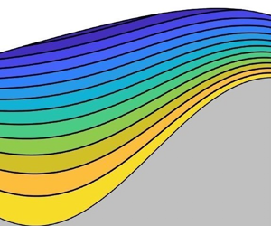



1. Introduction
Thin film flows are ubiquitous in the formation of functional surfaces/barriers, while playing a key role as part of numerous manufacturing/conversion process. In tandem, predicting their behaviour has motivated the work of experimentalists and modellers alike for decades. This remains true today, whether the objective is to produce defect free coated products as cheaply and as speedily as possible or to understand the source and means of suppressing free-surface disturbances when trying to extend established stability envelops to bring down production costs, etc.
For planar substrates and isothermal flow, the study of wave formation on the surface of falling liquid films began with Kapitza (Reference Kapitza1948), whose subsequent experiments (Kapitza & Kapitza Reference Kapitza and Kapitza1949) revealed the presence of steady waves on laminar films due to the classical hydrodynamic instability mode – a phenomenon recorded much earlier by Kirkbride (Reference Kirkbride1934). The apparent absence of surface waves at low Reynolds ( $Re$) numbers (Friedman & Miller Reference Friedman and Miller1941; Grimley Reference Grimley1945) popularised the existence of a critical Reynolds number,
 $Re_{crit}$, below which the film remained stable. Following measurements by Binnie (Reference Binnie1957) showing the average wavelength of instabilities was considerably larger than the average depth of the film, Benjamin (Reference Benjamin1957) provided a consensus via a long-wave approximation. Linearising the governing equations to first order he revealed
 $Re_{crit} = \frac {5}{4} \cot \beta$ in the absence of surface tension, where
 $\beta$ is the substrate inclination angle from the horizontal. Yih (Reference Yih1963) corroborated the above, providing a simplified mathematical proof of
 $Re_{crit}$ and showing the film's stability to be governed by surface waves rather than shear waves, at least for large
 $\beta$, in line with an earlier hypothesis proposed by Kapitza (Reference Kapitza1948).
The insights of Kapitza (Reference Kapitza1948) and Yih (Reference Yih1963) were subsequently exploited by Benney (Reference Benney1966) who performed the first nonlinear analysis using an evolution equation for the film thickness derived via a long-wave expansion. Whilst recovering  $Re_{crit}$ from the linearised theory, Benney omitted the effect of surface tension which meant his model failed to predict the progression of instabilities to a steady, finite-amplitude state as observed experimentally. Gjevik (Reference Gjevik1970) rectified this shortcoming by moving surface tension ahead of its formal order in the long-wave expansion. Measurements by Liu, Paul & Gollub (Reference Liu, Paul and Gollub1993) provided the first accurate experimental determination of
 $Re_{crit}$, showing the Benney equation is only valid close to
 $Re_{crit}$; an unphysical vanishing of solitary waves occurs outside this neighbourhood during finite-time simulations (Pumir, Manneville & Pomeau Reference Pumir, Manneville and Pomeau1983; Joo, Davis & Bankoff Reference Joo, Davis and Bankoff1991; Liu & Gollub Reference Liu and Gollub1994), limiting its use to periodic solutions (Lin Reference Lin1974; Nakaya Reference Nakaya1975, Reference Nakaya1989; Sivashinsky & Michelson Reference Sivashinsky and Michelson1983). Ooshida (Reference Ooshida1999) extended the Benney equation's plausible validity using a regularisation method but accurately resolving the film dynamics beyond
 $Re_{crit}$ demands a multi-variable model (Roberts Reference Roberts1996).
A two-equation depth-averaged model in terms of the flow rate and the film thickness was supplied by Shkadov (Reference Shkadov1967); coined the integral-boundary-layer (IBL) equations. The model utilised a self-similar parabolic velocity profile through the film but it failed to recover the correct expression for  $Re_{crit}$. Ruyer-Quil & Manneville (Reference Ruyer-Quil and Manneville1998) addressed this problem by expanding Shkadov's self-similar velocity profile to first order in the long-wave expansion, leading to a modified IBL model and recovery of the correct
 $Re_{crit}$. Following this, Ruyer-Quil & Manneville (Reference Ruyer-Quil and Manneville2000) presented an improved reduced model based on a polynomial expansion of the streamwise velocity, giving rise to what have become known as the weighted-IBL (WIBL) equations. In addition to predicting the correct
 $Re_{crit}$, the WIBL model does not display the unphysical behaviour beyond
 $Re_{crit}$ which plagues the Benney model, making it a popular choice ever since.
The case of isothermal film flow down non-planar substrate became of interest much later than its planar counterpart, with Tougou (Reference Tougou1978) and Wang (Reference Wang1981) showing  $Re_{crit}$ remained unchanged for small substrate waviness. Subsequently, Wang (Reference Wang1984) found the velocity through the film remained primarily parabolic when the film thickness is sufficiently smaller than the amplitude of the corrugated substrate – a feature corroborated experimentally (Scholle, Wierschem & Aksel Reference Scholle, Wierschem and Aksel2001a,Reference Scholle, Wierschem and Akselb). Subsequently, it was found substrate undulations lead to an increase in the film thickness and inertia can be neglected below the instability threshold (Zhao & Cerro Reference Zhao and Cerro1992; Wierschem, Scholle & Aksel Reference Wierschem, Scholle and Aksel2002). Moderate substrate corrugations have been discovered to delay the onset of surface instabilities when compared with their planar counterpart (Wierschem & Aksel Reference Wierschem and Aksel2003; Wierschem, Lepski & Aksel Reference Wierschem, Lepski and Aksel2005), with subsequent investigations (Oron & Henining Reference Oron and Henining2008; D'Alessio, Pascal & Jasmine Reference D'Alessio, Pascal and Jasmine2009; Cao, Vlachogiannis & Bontozoglou Reference Cao, Vlachogiannis and Bontozoglou2013; Pollak & Aksel Reference Pollak and Aksel2013) revealing a rich variety of stability phenomena including: short-wave transitions and isles of stability (Trifonov Reference Trifonov2014); the combined effect of corrugation amplitude and wavelength on flow stabilisation (Schörner, Reck & Aksel Reference Schörner, Reck and Aksel2015, Reference Schörner, Reck and Aksel2016); and culminating in the identification of six characteristic stability regimes for film flow over topography (Schörner & Aksel Reference Schörner and Aksel2018; Schörner et al. Reference Schörner, Reck, Aksel and Trifonov2018). Recently, Veremieiev & Wacks (Reference Veremieiev and Wacks2019) have shown the qualitative stability behaviour caused by substrate topography can be captured by a WIBL model.
Interestingly, the problem of film flow down both planar, and corrugated, uniformly heated substrates has received far less attention over the same period; initially from Goussis & Kelly (Reference Goussis and Kelly1991) who found two instability modes associated with thermo-capillarity: a long-wave variety linked to the hydrodynamic instability mode and a short-wave one. Given the temperature distribution within ‘a flat film flowing down a planar, uniformly heated incline’ is linear, it has become commonplace to initiate a long-wave expansion with an assumed linear temperature dependence through the film, even though it is impossible for the latter to satisfy all of the required boundary conditions. Proceeding in this way, the long-wave thermo-capillary mode was explored by Kalliadasis, Kiyashko & Demekhin (Reference Kalliadasis, Kiyashko and Demekhin2003b) and Kalliadasis et al. (Reference Kalliadasis, Demekhin, Ruyer-Quil and Velarde2003a) using a mixed Shkadov-weighted-residual model; however, it fails to retrieve  $Re_{crit}$ for uniformly heated substrate. The WIBL model derived by Ruyer-Quil et al. (Reference Ruyer-Quil, Scheid, Kalliadasis, Velarde and Zeytounian2005), using a self-similar linear temperature profile, overcame this problem, accurately predicting
 $Re_{crit}$ (Scheid et al. Reference Scheid, Ruyer-Quil, Kalliadasis, Velarde and Zeytounian2005); and was extended to the three-dimensional case (Scheid et al. Reference Scheid, Kalliadasis, Ruyer-Quil and Colinet2008). Saprykin et al. (Reference Saprykin, Trevelyan, Koopmans and Kalliadasis2007) were the first to consider the combined effect of topography and heating, employing a Benney-like long-wave expansion to model an evolving film on a horizontally aligned substrate. A self-similar linear temperature profile has been further utilised in WIBL models investigating heated, wavy substrate (D'Alessio et al. Reference D'Alessio, Pascal, Jasmine and Ogden2010; Ogden, D'Alessio & Pascal Reference Ogden, D'Alessio and Pascal2011); studies involving temperature-dependent fluid properties (Dávalos-Orozco Reference Dávalos-Orozco2012; Pascal, D'Alessio & Hasan Reference Pascal, D'Alessio and Hasan2018); and other heated film flow problems (Blyth & Bassom Reference Blyth and Bassom2012; Mukhopadhyay & Mukhopadhyay Reference Mukhopadhyay and Mukhopadhyay2020; Sterman-Cohen & Oron Reference Sterman-Cohen and Oron2020).
Problematically, a linear temperature dependence rapidly produces non-physical negative fluid temperatures in solitary wave simulations at moderate Péclet number; the fact most functional fluids exhibit large Péclet numbers underscores the importance of overcoming this barrier. Utilising a Galerkin projection of the energy equation, Trevelyan et al. (Reference Trevelyan, Scheid, Ruyer-Quil and Kalliadasis2007) showed the onset of negative temperature predictions can be stalled by a nonlinear temperature dependence and eliminated entirely by modifying the weight functions; however, the latter predictions are only in qualitative agreement with the full energy equation. Elsewhere, Chhay et al. (Reference Chhay, Dutykh, Gisclon and Ruyer-Quil2017) were able to evade the negative predictions of a linear temperature dependence by interchanging asymptotically equivalent terms in their averaged energy equation; instead constraining the temperature to follow the flat-film solution at large Péclet number. Thompson et al. (Reference Thompson, Gomes, Denner, Dallaston and Kalliadasis2019) adopted a linear temperature profile satisfying the Dirichlet and Neumann conditions at the free surface but not the substrate Dirichlet condition; in consequence, their ‘projection approach’ is only consistent at moderate Péclet numbers close to a critical value. The most promising results to date are those of Cellier & Ruyer-Quil (Reference Cellier and Ruyer-Quil2020), who applied a relaxation to the linear temperature dependence which promotes the nonlinear diffusion of heat inside the film. Proposing two models – a simpler single-variable one and a more complex two-variable one – they achieved good agreement with the full energy equation at moderate Péclet number, whilst concurrently delaying negative temperatures until large Péclet number. The current modelling aligns closely with that of Cellier & Ruyer-Quil (Reference Cellier and Ruyer-Quil2020) but unequivocally shows why the leading temperature expansion needs to be nonlinear.
To achieve this, the present work approaches the problem from a different perspective using substrate undulations to disturb the free surface. A rigorous analysis based on the modelling approach of Ruyer-Quil & Manneville (Reference Ruyer-Quil and Manneville2000) then reveals the primary nature of the fluid temperature to be nonlinear. The remainder of the paper proceeds as follows. The problem of interest is formulated in § 2 along with the derivation of a reduced three-equation model and associated linear stability analysis. A comprehensive set of results is provided and discussed in § 3, with conclusions drawn in § 4.
2. Problem formulation and modelling approach
2.1. Problem formulation
The problem of interest is that of a gravity-driven layer of Newtonian fluid, with constant density  $\rho$ and dynamic viscosity
 $\mu$, flowing over a uniformly heated, periodically corrugated rigid substrate inclined at an angle
 $\beta$ to the horizontal, as illustrated schematically in figure 1. The corresponding Cartesian coordinate system is orientated such that the
 $X$-axis points along and down the inclined substrate which is considered to be infinite and invariant in the
 $Y$-direction, with the
 $Z$-axis normal to it, rendering the principal problem two-dimensional. The substrate profile,
 $S(X)$, is measured relative to the
 $X$-axis and given by
 \begin{equation} S(X) = A \frac{ \left[ 1 + \cos \left( \dfrac{ 2 {\rm \pi}X }{ L } \right) \right] }{2}, \end{equation}
where  $A$ is the corrugation amplitude and
 $L$ its wavelength.
Schematic of film flow down a uniformly heated, wavy rigid substrate inclined at an angle  $\beta$ to the horizontal, showing the main geometrical features relative to the adopted coordinate system.

The film thickness,  $H(X,T)$, at a downstream location
 $X$, is the difference between the free-surface location,
 $Z = F(X,T)$, and the corrugation height,
 $Z = S(X)$. The temperature of the substrate,
 $\varTheta _s$, and that of the surrounding ambient gas,
 $\varTheta _a$, remain fixed and constant with the difference between them defined as
 $\varTheta _{\varDelta } = \varTheta _s - \varTheta _a$.
The equations governing the flow are the continuity and Navier–Stokes (NS) equations
 $$\begin{gather} \boldsymbol{\nabla} \boldsymbol{\cdot} \boldsymbol{U} = 0, \end{gather}$$
 $$\begin{gather}\rho \frac{ \textrm{D} \boldsymbol{U} }{ \textrm{D} T } ={-} \boldsymbol{\nabla} P + \rho \boldsymbol{{g}} + \mu \nabla^2 \boldsymbol{U}, \end{gather}$$
where  $\boldsymbol {U} = (U , W)^{\textrm {T}}$ and
 $P$ are the velocity and pressure fields, respectively,
 $\boldsymbol {\nabla } = ( \partial / \partial X , \partial / \partial Z )$ is the differential operator and
 $\boldsymbol {g} = \bar {g} ( \sin {\beta } , - \cos {\beta })^{\textrm {T}}$ is the acceleration due to gravity (with magnitude
 $\bar {g}$); together with a corresponding convection–diffusion equation representing the conservation of energy. For the case of no volumetric heating and negligible thermal viscous dissipation, the latter can be written in terms of the temperature field
 $\varTheta$ as
 \begin{equation} \rho C_P \frac{D \varTheta}{D T} = \kappa \nabla^2 \varTheta, \end{equation}
in which the heat capacity at constant pressure  $C_P$ and thermal conductivity
 $\kappa$ of the fluid are both assumed to remain constant.
The boundary conditions at the non-porous substrate include a no-slip and constant temperature requirement, namely
 \begin{equation} \boldsymbol{U} = 0,\quad \varTheta = \varTheta_s, \quad \text{at} \ Z = S(X). \end{equation}
The fluid is assumed to be non-volatile and  $\varTheta _{\varDelta }$ to be small enough that no evaporation of the liquid film takes place. Accordingly, the evolution of the free surface is described by the kinematic condition, given by
 \begin{equation} \frac{ \partial H }{ \partial T } + U \frac{ \partial F }{ \partial X } = W, \quad \text{at} \ Z = F(X,T), \end{equation}
where  $F(X,T) = S(X) + H(X,T)$. The normal and tangential force balance equations there are
 \begin{equation} \left. \begin{array}{ll} \hat{\boldsymbol{n}} \boldsymbol{\cdot} \boldsymbol{T} \boldsymbol{\cdot} \hat{\boldsymbol{n}} - \hat{\boldsymbol{n}} \boldsymbol{\cdot} \boldsymbol{\hat{T}} \boldsymbol{\cdot} \hat{\boldsymbol{n}} ={-} \sigma ( \boldsymbol{\nabla} \boldsymbol{\cdot} \hat{\boldsymbol{n}})\\ \ \ \hat{\boldsymbol{t}} \boldsymbol{\cdot} \boldsymbol{T} \boldsymbol{\cdot} \hat{\boldsymbol{n}} - \hat{\boldsymbol{t}} \boldsymbol{\cdot} \boldsymbol{\hat{T}} \boldsymbol{\cdot} \hat{\boldsymbol{n}} = \boldsymbol{\nabla} \sigma \boldsymbol{\cdot} \hat{\boldsymbol{t}} \end{array} \right\}\quad \text{at} \ Z = F(X,T), \end{equation}
where  $\boldsymbol {T} = - P \boldsymbol {I} + \mu [ ( \boldsymbol {\nabla } \boldsymbol {U} ) + ( \boldsymbol {\nabla } \boldsymbol {U} )^{\textrm {T}} ]$ and
 $\boldsymbol {\hat {T}} = - P_0 \boldsymbol {I}$ are the stress tensors of the fluid and ambient surrounding air, respectively;
 $P_0$ is the atmospheric pressure and
 $\boldsymbol {I}$ is the identity matrix. The normal and tangent unit vectors at the free surface are given by
 \begin{equation} \hat{\boldsymbol{n}} = \frac{1}{ \sqrt{ 1 + G } } \left( - \frac{ \partial F }{ \partial X } , 1 \right), \quad \hat{\boldsymbol{t}} = \frac{1}{ \sqrt{ 1 + G } } \left( 1 , \frac{ \partial F }{ \partial X } \right); \end{equation}
both of which include the surface curvature pre-factor,  $G = ( \partial F / \partial X )^2$. The surface tension of the film,
 $\sigma$, varies with
 $\varTheta$ in the following manner:
 \begin{equation} \sigma = \sigma_0 \left[ 1 + ( \varTheta - \varTheta_a ) \frac{ \partial \sigma }{ \partial \varTheta } \right] , \end{equation}
with  $\sigma _0$ the surface tension at temperature
 $\varTheta _a$; the surface tension gradient
 $\partial \sigma / \partial \varTheta$ is taken to be constant.
The heat transferred at the free surface follows Newton's law of cooling, which reads
 \begin{equation} - \kappa \hat{\boldsymbol{n}} \boldsymbol{\cdot} \boldsymbol{\nabla} \varTheta = \alpha (\varTheta - \varTheta_a), \quad \text{at} \ Z=F(X,T), \end{equation}
where  $\alpha$ is the liquid–gas heat transfer coefficient there and is valid as long as convective heat transfer is minimal, which can be expected when
 $\varTheta _{\varDelta }$ is small.
The following scalings are used to non-dimensionalise the governing equations and boundary conditions, (2.1)–(2.9):
 \begin{equation} \left. \begin{array}{ccc@{}} X = L x, & Z = H_0 z, & T = \dfrac{L}{U_0} t,\\ U = U_0 u, & W = \dfrac{ H_0 U_0 }{ L } w, & \varTheta = \varTheta_{\varDelta} \theta + \varTheta_a,\\ S = H_0 s & H = H_0 h, & P = \dfrac{ \mu U_0 L }{ H_0^2 } p, \end{array} \right\}, \end{equation}
with lowercase letters representing dimensionless variables. The vertical length scale,  $H_0$, corresponds to the Nusselt film thickness
 \begin{equation} H_0 = \left( \frac{ 3 \mu \dot{V_0} }{ \rho \bar{g} \sin{\beta} } \right)^{1/3}, \end{equation}
while the free-surface velocity for a flat film,  $U_0 = 3 \dot {V_0} / 2 H_0$, is taken as the velocity scale. The two are linked through the streamwise flow rate per unit cross-sectional width,
 $\dot {V_0}$.
Applying the scalings leads to the following dimensionless substrate profile:
 \begin{equation} s(x) = \frac{A}{H_0} \frac{[ 1 + \cos ( 2 {\rm \pi}x )] }{2} \end{equation}
and dimensionless governing equations
 $$\begin{gather} \frac{ \partial u }{ \partial x } + \frac{ \partial w }{ \partial z } = 0, \end{gather}$$
 $$\begin{gather}{\epsilon} Re \left[ \frac{ \partial u }{ \partial t } + u \frac{ \partial u }{ \partial x } + w \frac{ \partial u }{ \partial z } \right] ={-} \frac{ \partial p }{ \partial x } + 2 + {\epsilon}^2 \frac{ \partial^2 u }{ \partial x^2 } + \frac{ \partial^2 u }{ \partial z^2 },\end{gather}$$
 $$\begin{gather}{\epsilon}^3 Re \left[ \frac{ \partial w }{ \partial t } + u \frac{ \partial w }{ \partial x } + w \frac{ \partial w }{ \partial z } \right] ={-} \frac{ \partial p }{ \partial z } - 2 {\epsilon} \cot \beta + {\epsilon}^2 \frac{ \partial }{ \partial x } \left[ {\epsilon}^2 \frac{ \partial w }{\partial x } + \frac{ \partial u }{ \partial z } \right]+ 2 {\epsilon}^2 \frac{ \partial^2 w }{\partial z^2 },\end{gather}$$
 $$\begin{gather}{\epsilon} Re\,Pr \left[ \frac{ \partial \theta }{ \partial t } + u \frac{ \partial \theta }{ \partial x } + w \frac{ \partial \theta }{ \partial z } \right] = {\epsilon}^2 \frac{ \partial^2 \theta }{ \partial x^2 } + \frac{ \partial^2 \theta }{ \partial z^2 },\end{gather}$$
featuring the following dimensionless groups: the shallowness parameter,  ${\epsilon } = H_0 / L$; the Reynolds number,
 $Re = \rho U_0 H_0 / \mu$; the Prandtl number,
 $Pr = ( \mu C_P ) / \kappa$.
The dimensionless boundary conditions at the substrate,  $z = s(x)$, read
 \begin{equation} u|_{z=s} = w|_{z=s} = 0,\quad \theta |_{z=s}= 1, \end{equation}
while scaling and expanding the boundary conditions at the free surface,  $z = f(x,t)$, leads to the following expressions:
 $$\begin{gather} w|_{z=f} = \frac{ \partial h }{ \partial t } + u|_{z=f} \frac{ \partial f }{ \partial x },\end{gather}$$
 $$\begin{gather}p|_{z=f} = p_0 - \left. 2 {\epsilon}^2 \left[ \frac{( 1 - {\epsilon}^2g) \dfrac{ \partial u }{ \partial x } + \dfrac{ \partial f }{ \partial x } \left[ {\epsilon}^2 \dfrac{ \partial w }{ \partial x } + \dfrac{ \partial u }{ \partial z } \right] }{ 1 + {\epsilon}^2 g } \right] \right|_{z=f}- \frac{ {\epsilon}^3 ( 1 - Ma \vartheta ) \dfrac{ \partial^2 f }{ \partial x^2 } }{ Ca [ 1 + {\epsilon}^2g ]^{3/2} }, \end{gather}$$
 $$\begin{gather}\left. \left[ {\epsilon}^2 \frac{ \partial w }{ \partial x } + \frac{ \partial u }{ \partial z } \right] \right|_{z=f} = 4 \frac{ \left. {\epsilon}^2 \dfrac{ \partial f }{ \partial x } \dfrac{ \partial u }{ \partial x } \right|_{z=f} }{ 1 - {\epsilon}^2 g } - \left. {\epsilon} \frac{Ma}{Ca} \frac{ \sqrt{ 1 + {\epsilon}^2 g } }{ 1 - {\epsilon}^2 g } \left[ \frac{ \partial \theta }{ \partial x } + \frac{ \partial f }{ \partial x } \frac{ \partial \theta }{ \partial z } \right] \right|_{z=f}, \end{gather}$$
 $$\begin{gather}\left. \frac{ \partial \theta }{ \partial z } \right|_{z=f} = \left. {\epsilon}^2 \frac{ \partial f }{ \partial x } \frac{ \partial \theta }{ \partial x } \right|_{z=f} - Bi \vartheta \sqrt{ 1 + {\epsilon}^2 g }. \end{gather}$$
These include the dimensionless free-surface profile,  $f(x,t) = s(x) + h(x,t)$, and temperature,
 $\vartheta = \theta |_{z=f}$, together with the dimensionless surface curvature pre-factor,
 $g = ( \partial f / \partial x )^2$. In addition, they contain the following additional dimensionless groups: Capillary number,
 $Ca = \mu U_0 / \sigma _0$; Marangoni number,
 $Ma = \varTheta _{\varDelta } ( - \partial \sigma / \partial \varTheta )$; Biot number,
 $Bi = \alpha H_0 / \kappa$.
The fluid pressure is obtained by integrating equation (2.13c) between  $z$ and
 $z = f(x,t)$ with the upper limit of integration given by (2.15b), leading to
 \begin{align} p &= p_0+ 2 {\epsilon} ( f - z ) \cot \beta - {\epsilon}^2 \frac{ \partial u }{ \partial x } - {\epsilon}^2 \frac{ \partial }{ \partial x } ( u|_{z=f} ) - { \epsilon}^3 \frac{ \partial }{ \partial x } \left[ \frac{ (1 - Ma \vartheta ) }{ Ca } \frac{ \dfrac{ \partial f }{ \partial x } }{ \sqrt{ 1 + {\epsilon}^2 g } } \right] \nonumber\\ &\quad + {\epsilon}^3 Re \int^{f}_{z} \left[ \frac{ \partial w }{ \partial t } + \frac{ \partial }{ \partial x} ( u w ) + \frac{ \partial }{ \partial z } ( w^2 )\right] \textrm{d}z - {\epsilon}^4 \frac{ \partial }{ \partial x } \int^{f}_{z} \frac{ \partial w }{ \partial x } \, \textrm{d}z, \end{align}
a complete derivation of which is provided in the online supplementary material available at https://doi.org/10.1017/jfm.2021.920.
2.2. Reduced asymptotic model
Solving the full equation set (2.13)–(2.15) represents a daunting task due to the a priori unknown location of the free surface. Accordingly, an asymptotic model of reduced dimensionality is derived following the modelling approach of Ruyer-Quil & Manneville (Reference Ruyer-Quil and Manneville2000). Proceeding in this way is superior to the gradient expansion of Benney (Reference Benney1966) because it captures the distortion of the primary parabolic flow as deviations manifest.
Gravity-driven film flow is well suited to analysis via a long-wave expansion due to the predominance of surface tension with regard to the film stability, in that long waves are commonly the most unstable modes (Oron, Davis & Bankoff Reference Oron, Davis and Bankoff1997). Therefore, it is reasonable to assume quantities vary slowly in time and in the  $x$-direction, which is to say derivatives with respect to
 $x$ and
 $t$ are small. The smallness of space–time derivatives in the present scaling is represented by the shallowness parameter,
 ${\epsilon } < 1$, with the order of such terms in the long-wave expansion given by the power of the scaling factor,
 ${\epsilon }^n$. In contrast, gradients with respect to the
 $z$-coordinate can be considered large. Accordingly, and on the assumption that
 $u$ and
 $\theta$ are infinitely differentiable with respect to
 $z$, the fluid velocity and temperature are expanded as infinite series which take the form
 \begin{equation} u = \sum^{\infty}_{j=0} a_j (x,t) \phi_j (z),\quad \theta = 1 + \sum^{\infty}_{j=0} b_j (x,t) \phi_j (z), \end{equation}
where  $\{ a_j , b_j \}$ denote unknown expansion coefficients and
 $\phi _j = ( z - s)^{j+1}$ are basis functions selected to automatically satisfy the substrate boundary conditions (2.14); thus, expansions (2.17) represent power series in
 $z$ centred around the substrate position,
 $s ( x )$. An expansion of the vertical flow velocity is unnecessary since an expression for
 $w$ in terms of
 $u$ can be found by expressing the continuity equation (2.13) in the form
 \begin{equation} w ={-} \int^{z}_{s} \frac{ \partial u }{ \partial x }\, \textrm{d}z. \end{equation}
An expansion of the fluid pressure is likewise redundant since an algebraic expression – (2.16) – exists.
Representing  $u$ and
 $\theta$ as power series in
 $z$ enables a reduction in dimensionality because substituting the expansions (2.17) into the governing equations (2.13) converts each equation into an infinite sum of
 $\phi _j$; this can be represented mathematically by
 \begin{equation} R_{({-}1)} (x,t) + R_{0} (x,t) \phi_0 ( \hat{z} ) + R_{1} (x,t) \phi_1 ( \hat{z} ) + \cdots+ R_{J} (x,t) \phi_J ( \hat{z} ) + \cdots= 0 ,\end{equation}
in which the  $\phi _j$ depend on the reduced variable
 $\hat {z} = ( z - s )$ whilst the coefficients
 $R_j$ are functions of
 $( x , t )$. A reduction in dimensionality follows because: (i) (2.19) must be satisfied across the whole domain of
 $\varOmega = \{ x \in [ 0 , 1 ] , \ \hat {z} \in [ 0 , h ] \}$; and (ii)
 $\{ 1 , \phi _j \}$ constitute the monomial basis of
 $\hat {z}$ and are therefore linearly independent. Consequently, (2.19) can only be satisfied if
 $R_j (x,t) = 0$ for
 $j = -1 , 0 , 1 ,\ldots, J ,\ldots, \infty$. This leads to a reduced equation set made up of the residuals
 $R_j (x,t)$ for
 $j = -1 , 0 , 1 ,\ldots, J ,\ldots, \infty$ and the free-surface boundary conditions (2.15) which are functions of
 $( x , t )$ but independent of
 $z$. The reduced equations are satisfied by solutions to the expansion coefficients
 $\{ a_j , b_j \}$.
Needless to say, solving an infinite number of residual equations would be impractical, and so truncations of expansions (2.17) are required; thus, the solutions to  $u$ and
 $\theta$ sought via this approach are approximate rather than exact. Nevertheless, it is at least possible to find asymptotically equivalent solutions within the framework of a long-wave expansion. The smallness of derivatives with respect to
 $( x , t )$ means approximating such terms using truncations of expansions (2.17) leads to asymptotic solutions which are equivalent to the exact solutions within a bounded parameter space. The truncations needed to approximate space–time derivatives are found from a gradient expansion of the fluid velocity and temperature, taking the form
 $( u , \theta ) = ( u_0 , \theta _0 ) + {\epsilon } ( u_1 , \theta _1 ) + {\epsilon }^2 ( u_2 , \theta _2 ) + \cdots$.
The first step is to find  $( u_0 , \theta _0)$. A potential starting point are the analytical solutions for the case of ‘a flat film flowing down a planar, uniformly heated incline’, found by setting
 ${\epsilon } = 0$ in (2.13)–(2.15), and attributed to Nusselt (Reference Nusselt1916), who first found such an expression for the velocity profile through an isothermal flat film; they read
 \begin{equation} u_{Nu} = ( z - s ) ( s + 2 h - z ),\quad \theta_{Nu} = 1 + \left( \frac{1}{1 + Bih} - 1 \right) \frac{ ( z - s ) }{ h }. \end{equation}
Equations (2.20) represent exact solutions which are only strictly valid when  ${\epsilon } = 0$; indeed, setting
 $( u_0 , \theta _0 ) = ( u_{Nu} , \theta _{Nu})$ leads to a Benney expansion in terms of the film thickness
 $( h )$. The derivation of a reduced asymptotic model which accurately resolves the film dynamics beyond the trivial case requires expansions whose forms are invariant with respect to
 ${\epsilon }$ – consider the self-similarity function in a Blasius boundary layer (Blasius Reference Blasius1908) – and necessitates a multi-modal parametrisation of the reduced equations (Roberts Reference Roberts1996).
A better starting point is to identify which of the expansion coefficients  $\{ a_j ,b_j \}$ can enter at leading order in the gradient expansion, and use these expansion coefficients
 $\{ a_j , b_j \}$ to represent the amplitudes of the primary flow and heat transfer, i.e.
 $( u_0 , \theta _0 )$. This is accomplished by deriving a set of conditions from the governing equations for the heated film case which isolate the individual expansion coefficients so their order may be inferred from other terms present in the equations (Ruyer-Quil & Manneville Reference Ruyer-Quil and Manneville2000). Since expansions (2.17) are power series in
 $z$,
 $\{ a_j , b_j \}$ can be isolated by differentiating equations (2.13b,d)
 $n - 2$ times with respect to
 $z$ and only with respect to
 $z$; this gives
 $$\begin{gather} {\epsilon} Re \frac{ \partial^{n-2} }{ \partial z^{n-2} } \left[ u \frac{ \partial u }{ \partial x } + w \frac{ \partial u }{ \partial z } + \frac{ \partial u }{ \partial t }\right] = \frac{ \partial^n u }{ \partial z^n }, \end{gather}$$
 $$\begin{gather}{\epsilon} Re\, Pr \frac{ \partial^{n-2} }{ \partial z^{n-2} } \left[ u \frac{ \partial \theta }{ \partial x } + w \frac{ \partial \theta }{ \partial z } + \frac{ \partial \theta }{ \partial t } \right] = \frac{ \partial^n \theta }{ \partial z^n }, \end{gather}$$
where it has been assumed  $Re \sim Pr \sim {O} (1)$ and all terms of
 ${\sim}{O} ( {\epsilon }^2 )$ and higher have been discarded. At this point it is only necessary to determine which
 $\{ a_j , b_j \}$ are of at least first order in the long-wave expansion. Considering all powers of
 $z$, the infinite expansions (2.17) yield the following conditions when substituted into (2.21):
 \begin{align} &\boldsymbol{R}
\left[\sum^{n-2}_{k=0} \left( \sum^{\infty}_{j=0} a_j
\phi_{j-n+k+2} \prod^{n-k-2}_{i=0} \frac{ ( \,j - i + 2 )
}{ ( \,j + 2 ) } \right) \left(
\sum^{\infty}_{j=0} \frac{ \partial }{ \partial x } [
\boldsymbol{r}_j \phi_{j-k} ] \prod^{k}_{i=0} \frac{ ( \,j
- i + 2 ) }{ ( \,j + 2 ) } \right) \right. \nonumber\\
&\quad - \sum^{n-2}_{k=0}\left(\sum^{\infty}_{j=0} \frac{
\dfrac{ \partial }{ \partial x } [ a_j \phi_{j-n+k+3} ] }{
( \,j + 2 ) } \prod^{n-k-2}_{i=0} \frac{ ( \,j - i + 3 ) }{
( \,j + 3 ) }\right) \left(
\sum^{\infty}_{j=0} \boldsymbol{r}_j \phi_{j-k-1}
\prod^{k+1}_{i=0} \frac{ ( \,j - i + 2 ) }{ ( \,j + 2 ) }
\right) \nonumber\\ &\quad \left.+ \sum^{\infty}_{j=0}
\frac{ \partial \boldsymbol{r}_j }{ \partial t }
\phi_{j-n+2} \prod^{n-2}_{i=0} \frac{ ( \,j - i + 2 ) }{ (
\,j + 2 ) } \right] = \sum^{\infty}_{j=0} \boldsymbol{r}_j
\phi_{j-n} \prod^{n}_{i=0} \frac{ ( \,j - i + 2 ) }{ ( \,j
+ 2 ) }, \end{align}
for (i)  $\boldsymbol {r}_j = a_j$ with
 $\boldsymbol {R} = {\epsilon } Re$, and (ii)
 $\boldsymbol {r}_j = b_j$ with
 $\boldsymbol {R} = {\epsilon } Re\, Pr$.
The right-hand side of (2.22) is proportional to  $\{ a_{n-1} , b_{n-1} \}$ because the repeated product only leaves terms of
 $\{ a_j , b_j \}$ satisfying the inequality
 $j - n + 2 > 0$, simplifying to
 $j \geq n - 1$ as
 $\{ \,j , n \} \in \mathbb {Z}^+$. Meanwhile, the left-hand side of (2.22) is of at least first order in the long-wave expansion due to the presence of space–time derivatives. Stipulating that both sides of (2.22) be of equivalent orders requires
 $\{ a_{n-1} , b_{n-1} \}$ to be of at least first order. Equations (2.21)–(2.22) hold for
 $n > 2$: constants of integration appear when
 $n \leq 2$; implying all
 $\{ a_j , b_j \}$ for
 $j \geq 2$ are of at least first-order; leaving only
 $\{ a_0 , a_1 , b_0 , b_1 \}$ to be candidates of order unity,
 ${\sim}{O} ( 1 )$, and to represent the amplitudes of the primary flow and heat transfer, i.e.
 $( u_0 , \theta _0 )$.
On the conjecture that  $\{ a_0 , a_1 , b_0 , b_1 \}$ are the leading expansion coefficients, attention is directed to expressing
 $\{ a_0 , a_1 , b_0 , b_1 \}$ in terms of physically measurable parameters and making sure the power series (2.17) satisfy all of the boundary conditions (2.14)–(2.15). Consequently, a variable transformation of the following form is sought:
 \begin{equation} (u , w , \theta) \to ( q , h , \vartheta ), \end{equation}
where  $q$ is the streamwise flow rate,
 $h$ is the film thickness and
 $\vartheta$ is the free-surface temperature. The flow rate
 $( q )$ is a controllable physical quantity, whilst the film thickness
 $( h )$ and free-surface temperature
 $( \vartheta )$ already appear in the free-surface boundary conditions (2.15). The variable transformation can be easily accomplished by finding the expressions which relate
 $\{ a_j , b_j \}$ to
 $( q , h , \vartheta )$; in addition to providing physical context, the resulting expressions describe how the velocity expansion coefficients
 $\{ a_j \}$ and the temperature expansion coefficients
 $\{ b_j \}$ linearly depend upon one another, respectively.
The fluid velocity and temperature are related to the streamwise flow rate and free-surface temperature, respectively, by
 \begin{equation} q = \int^{f}_{s} u \, \textrm{d}z, \quad \vartheta = \theta |_{z=f}. \end{equation}
Substituting expansions (2.17) into definitions (2.24) leads to the following relationships:
 \begin{equation} q = \sum^{\infty}_{j=0} \frac{ h^{j+2} }{ ( \,j + 2) } a_j, \quad \vartheta - 1 = \sum^{\infty}_{j=0} h^{j+1} b_j, \end{equation}
which form the first set of conditions relating  $\{ a_j , b_j \}$ to
 $( q , h , \vartheta )$.
The decision to centre the power series about  $s ( x )$ ensures the substrate boundary conditions (2.14) are automatically satisfied by expansions (2.17); however, the free-surface boundary conditions (2.15) are not. Substituting expressions (2.17)–(2.18) into (2.15) yields supplementary conditions which complement those in (2.25). Approximating the kinematic condition (2.15a) using (2.17)–(2.18), and simplifying via condition (2.25), leads to the integral form of the kinematic condition
 \begin{equation} \frac{ \partial h }{ \partial t } + \frac{ \partial q }{ \partial x } = 0, \end{equation}
describing the relationship between film thickness and flow rate. Equation (2.26) is universal for non-volatile, incompressible film flow and can be derived by integrating the continuity equation (2.13a) between  $z = s(x)$ and
 $z = f(x,t)$, with the lower and upper bounds of the integration given by (2.14a) and (2.15a), respectively, followed by simplifying via the Leibniz integral rule and streamwise flow rate definition.
Since both the  $z$-momentum equation (2.13c) and the normal stress condition (2.15b) are eliminated from the equation set (2.13)–(2.15) following a substitution of the fluid pressure – (2.16) – into the
 $x$-momentum – (2.13); only the shear stress (2.15c) and heat flux (2.15d) boundary conditions remain. With reference to the variable transformation of (2.23), boundary conditions (2.15c,d) can be re-written as
 $$\begin{gather} \left. \frac{ \partial u }{ \partial z } \right|_{z=f} = \frac{ 2 {\epsilon}^2 \dfrac{ \partial f }{ \partial x } \left.\dfrac{ \partial u }{ \partial x } \right|_{z=f} }{ 1 - {\epsilon}^2 g } + \dfrac{ {\epsilon}^2 \left[ \dfrac{ \partial^2 q }{ \partial x^2 } - u|_{z=f} \dfrac{ \partial^2 f }{ \partial x^2 } \right] }{ 1 + {\epsilon}^2 g } - \dfrac{ {\epsilon} \dfrac{Ma}{Ca} \dfrac{ \partial \vartheta }{ \partial x } }{ \sqrt{ 1 + {\epsilon}^2 g } [ 1 - {\epsilon}^2 g ] }, \end{gather}$$
 $$\begin{gather}\left. \frac{ \partial \theta }{ \partial z } \right|_{z=f} = \frac{ {\epsilon}^2 \dfrac{ \partial f }{ \partial x } \dfrac{ \partial \vartheta }{ \partial x } }{ 1 + {\epsilon}^2 g } - \frac{ Bi \vartheta }{ \sqrt{ 1 + {\epsilon}^2 g} }, \end{gather}$$
utilising  $\partial w / \partial z = - \partial u / \partial x$ via the continuity equation (2.13a),
 $w|_{z=f}$ from the kinematic condition (2.15a) and the total spatial derivatives defined along the free surface, namely
 $$\begin{gather} \frac{ \partial \vartheta }{ \partial x } = \left. \frac{ \partial \theta }{ \partial x } \right|_{z=f} + \frac{ \partial f }{ \partial x } \left. \frac{ \partial \theta }{ \partial z } \right|_{z=f,} \end{gather}$$
 $$\begin{gather}\frac{ \partial }{ \partial x } ( u|_{z=f} ) = \left. \frac{ \partial u }{ \partial x } \right|_{z=f} + \frac{ \partial f }{ \partial x } \left. \frac{ \partial u }{ \partial z } \right|_{z=f,} \end{gather}$$
 $$\begin{gather}\frac{ \partial }{ \partial x } ( w|_{z=f} ) = \left. \frac{ \partial w }{ \partial x } \right|_{z=f} + \frac{ \partial f }{ \partial x } \left. \frac{ \partial w }{ \partial z } \right|_{z=f}. \end{gather}$$
Substituting expansions (2.17) into the left-hand side of (2.27a,b) (within the framework of the long-wave expansion, space–time derivatives on the right-hand side of (2.27) are approximated via recursion using truncations of expansions (2.17)) yields
 \begin{align} \sum^{\infty}_{j=0} ( \,j + 1 ) h^j a_j &= \frac{ 2 {\epsilon}^2 \dfrac{ \partial f }{ \partial x } \left. \dfrac{ \partial u }{ \partial x } \right|_{z=f} }{ 1 - {\epsilon}^2 g } + \dfrac{ {\epsilon}^2 \left[ \dfrac{ \partial^2 q }{ \partial x^2 } - u|_{z=f} \dfrac{ \partial^2 f }{ \partial x^2 } \right] }{ 1 + {\epsilon}^2 g }\nonumber\\ &\quad- \frac{ {\epsilon} \dfrac{Ma}{Ca} \dfrac{ \partial \vartheta }{ \partial x } }{ \sqrt{ 1 + {\epsilon}^2 g } [ 1 - {\epsilon}^2 g ]}, \end{align}
 \begin{align} \sum^{\infty}_{j=0} ( \,j + 1 ) h^j b_j &= \frac{ {\epsilon}^2 \dfrac{ \partial f }{ \partial x } \dfrac{ \partial \vartheta }{ \partial x } }{ 1 + {\epsilon}^2 g } - \frac{ Bi \vartheta }{ \sqrt{ 1 + {\epsilon}^2 g } }, \end{align}
respectively, which form the second set of conditions relating  $\{ a_j , b_j \}$ to
 $( q , h , \vartheta )$.
Thus far, the presumption from (2.22) is that  $\{ a_0 , a_1 , b_0 , b_1 \}$ are the leading expansion coefficients, and four relationships linking
 $\{ a_j , b_j \}$ to
 $( q , h ,\vartheta )$ have been derived – (2.25) and (2.29); with an additional condition linking the film thickness and flow rate in (2.26). Therefore, solving for
 $\{ a_0 , a_1 , b_0 , b_1 \}$ in (2.25) and (2.29) returns expressions for them in terms of
 $( q , h , \vartheta, a_j , b_j )$ for
 $j \geq 2$, which read
 \begin{align} a_0 &=\frac{ 3 q }{ 2h^3 } (2h) + \frac{1}{2} \sum^{\infty}_{j=2} \frac{ ( \,j + 4 ) ( \,j -1 ) }{ ( \,j + 2 ) } h^j a_j \nonumber\\ &\quad - \frac{1}{2} \left[ \frac{ \left. 2 {\epsilon}^2 \dfrac{ \partial f }{ \partial x } \dfrac{ \partial u }{ \partial x } \right|_{z=f} - \dfrac{ {\epsilon} \frac{Ma}{Ca} \frac{ \partial \vartheta }{\partial x } }{ \sqrt{ 1 + {\epsilon}^2 g } } }{ 1 - {\epsilon}^2 g } + \frac{ {\epsilon}^2 \left[ \dfrac{ \partial^2 q }{ \partial x^2 } - u|_{z=f} \dfrac{ \partial^2 f }{ \partial x^2 } \right] }{ 1 + {\epsilon}^2 g } \right], \end{align}
 \begin{align} a_1 &={-} \frac{3 q}{2h^3} - \frac{3}{4h} \sum^{\infty}_{j=2} \frac{ j ( \,j + 3 ) }{ ( \,j + 2 ) } h^j a_j \nonumber\\ &\quad + \frac{3}{4h} \left[ \frac{ \left. 2 {\epsilon}^2 \dfrac{ \partial f }{ \partial x } \dfrac{ \partial u }{ \partial x } \right|_{z=f} - \dfrac{ {\epsilon} \frac{Ma}{Ca} \frac{ \partial \vartheta }{ \partial x } }{ \sqrt{ 1 + {\epsilon}^2 g } } }{ 1 - {\epsilon}^2 g } + \frac{ {\epsilon}^2 \left[ \dfrac{ \partial^2 q }{ \partial x^2 } - u|_{z=f} \dfrac{ \partial^2 f }{ \partial x^2 } \right] }{ 1 + {\epsilon}^2 g } \right], \end{align}
 $$\begin{align} b_0 &= \frac{ ( \vartheta - 1 ) }{ h } + \left[ \frac{ ( \vartheta - 1 ) }{ h } - \frac{ {\epsilon}^2 \dfrac{ \partial f }{ \partial x } \dfrac{ \partial \vartheta }{ \partial x } }{ 1 + {\epsilon}^2 g } + \frac{ Bi \vartheta }{ \sqrt{ 1 + {\epsilon}^2 g } } \right] + \sum^{\infty}_{j=2} ( \,j - 1 ) h^j b_j, \end{align}$$
 $$\begin{align}b_1 &={-} \frac{1}{h} \left[ \frac{ \left( \vartheta - 1 \right) }{ h } - \frac{ {\epsilon}^2 \dfrac{ \partial f }{ \partial x } \dfrac{ \partial \vartheta }{ \partial x } }{ 1 + {\epsilon}^2 g } + \frac{ Bi \vartheta }{ \sqrt{ 1 + {\epsilon}^2 g } } \right] - \frac{1}{h} \sum^{\infty}_{j=2} j h^j b_j, \end{align}$$
where  $( q , h , \vartheta, Ma, Ca, Bi ) \sim {O} (1)$ and
 $\{ a_j , b_j \} \sim {O} ( {\epsilon }^n )$ for
 $j \geq 2$ and
 $n\geq 1$.
This is advantageous because: (i) replacing  $\{ a_0 , a_1 , b_0 , b_1 \}$ in the expansions of
 $( u ,\theta )$ – (2.17) – with the identities above allows the power series to satisfy not only the substrate boundary conditions but also to algebraically satisfy those at the free surface – leaving only the
 $x$-momentum (2.13b) and energy (2.13d) equations to be satisfied; and (ii) the leading truncations of the gradient expansion,
 $( u_0 , \theta _0 )$, can now be found. The identities of
 $\{ a_0 , a_1 \}$ are asymptotically equivalent, in the long-wave limit, to the amplitude of the parabolic velocity profile derived by Ruyer-Quil et al. (Reference Ruyer-Quil, Scheid, Kalliadasis, Velarde and Zeytounian2005); meanwhile, the identities of
 $\{ b_0 , b_1 \}$ can be compared with the temperature expansions of Trevelyan et al. (Reference Trevelyan, Scheid, Ruyer-Quil and Kalliadasis2007) and Cellier & Ruyer-Quil (Reference Cellier and Ruyer-Quil2020). In the work of Trevelyan et al. (Reference Trevelyan, Scheid, Ruyer-Quil and Kalliadasis2007), the expansion coefficients were not assigned any order with respect to
 ${\epsilon }$ but an emphasis was placed on the cubic temperature coefficient to ease comparison with a Benney expansion of the fluid temperature; accordingly, a temperature expansion with the same form as (5.10b) in Trevelyan et al. (Reference Trevelyan, Scheid, Ruyer-Quil and Kalliadasis2007) can be retrieved by solving for
 $b_2$ instead of
 $b_1$ in (2.30c,d). Unfortunately, the single-variable heat transfer model proposed by Trevelyan et al. (Reference Trevelyan, Scheid, Ruyer-Quil and Kalliadasis2007) is inconsistent with the long-wave expansion because it was derived following the Galerkin method; a consistent evolution equation for
 $\vartheta$ can be obtained by following either the current approach or that of Cellier & Ruyer-Quil (Reference Cellier and Ruyer-Quil2020). In a similar fashion, a temperature expansion with the same form as Cellier & Ruyer-Quil (Reference Cellier and Ruyer-Quil2020) can be retrieved by introducing the evaluation of the energy equation (2.13c) at the free surface as a supplementary boundary condition; the latter can be written as
 \begin{align} \left. \frac{ \partial^2 \theta }{ \partial z^2 } \right|_{z=f} = \frac{ {\epsilon} Re\,Pr \left[ \dfrac{ \partial \vartheta }{ \partial t } + u|_{z=f} \dfrac{ \partial \vartheta }{ \partial x } \right] + {\epsilon}^2 \left[ \dfrac{ \partial^2 f }{ \partial x^2 } \left. \dfrac{ \partial \theta }{ \partial z } \right|_{z=f} + 2 \dfrac{ \partial f }{ \partial x } \dfrac{ \textrm{d} }{ {\textrm{d}\kern0.7pt x} } \left( \left. \dfrac{ \partial \theta }{ \partial z } \right|_{z=f} \right) - \dfrac{ \partial^2 \vartheta }{ \partial x^2 } \right] }{ 1 + {\epsilon}^2 g }. \end{align}
Substituting the power series (2.17b) into the left-hand side of (2.31), with  $\{ b_0 , b_1 \}$ given by (2.30c,d), and solving for
 $b_2$ returns a temperature expansion with the same form as Cellier & Ruyer-Quil (Reference Cellier and Ruyer-Quil2020). Equation (2.31) is left out of the current analysis because the space–time derivatives composing the right-hand side indicate it is purely a first-order contribution; the present objective is to find
 $( u_0 , \theta _0 )$.
To write the expansions at leading order, expressions (2.30) are substituted into the power series (2.17) and all terms of order  ${\sim}{O}( {\epsilon })$ and higher are discarded; this yields
 $$\begin{gather} u_0 = \frac{3 q}{2h^3} ( z - s ) ( s + 2h - z ), \end{gather}$$
 $$\begin{gather}\theta_{para} = 1 + \frac{ ( \vartheta - 1 ) }{ h } ( z - s ) + \frac{1}{h} \left[ \frac{ ( \vartheta - 1 ) }{ h } + \frac{ Bi \vartheta }{ \sqrt{ 1 + {\epsilon}^2 g } } \right] ( z - s ) ( s + h - z ), \end{gather}$$
in which surface curvature  $( {\epsilon }^2 g )$ has been retained, so its effect on the heat transfer through the free surface is accurately captured, but thermo-capillarity has been excluded as the Marangoni effect is purely a deviant mechanism in uniformly heated film flow. The leading temperature expansion (2.32b) is labelled
 $\theta _{para}$ because it is parabolic and thus a departure from the linear temperature expansion used by Kalliadasis et al. (Reference Kalliadasis, Demekhin, Ruyer-Quil and Velarde2003a,Reference Kalliadasis, Kiyashko and Demekhinb), Ruyer-Quil et al. (Reference Ruyer-Quil, Scheid, Kalliadasis, Velarde and Zeytounian2005), D'Alessio et al. (Reference D'Alessio, Pascal, Jasmine and Ogden2010) and Sterman-Cohen & Oron (Reference Sterman-Cohen and Oron2020).
A long-standing assumption in the modelling of heated film flow has been that the leading approximation to the temperature expansion must be linear because the Nusselt temperature distribution – (2.20b) – is linear. This line of thinking would demand the parabolic correction in (2.32b) be of first order with respect to  ${\epsilon }$ and reduce the leading temperature expansion to the linear form offered by Ruyer-Quil et al. (Reference Ruyer-Quil, Scheid, Kalliadasis, Velarde and Zeytounian2005). There is merit in this assumption because the parabolic coefficient
 $b_1$ does tend to zero in the case of a ‘flat film flowing down a planar, uniformly heated incline’ (due to the free-surface temperature approaching its flat-film solution), or expressed mathematically
 \begin{equation} \lim_{{\epsilon} \to 0 } \vartheta = \frac{ 1 }{ 1 + Bi h } + {O} ( {\epsilon} ), \quad \lim_{{\epsilon} \to 0} \left[ \frac{ ( \vartheta - 1 ) }{ h } + \frac{ Bi \vartheta }{ \sqrt{ 1 + {\epsilon}^2 g } } \right] + {O} ( {\epsilon} ) = 0. \end{equation}
Nevertheless, there are two issues with this assumption: (i) the parabolic correction in (2.32b) contains only quantities which are of order unity,  $( h , \vartheta, Bi ) \sim {O} (1)$; and (ii) a linear temperature approximation at leading order produces inaccurate predictions except when the free-surface temperature
 $( \vartheta )$ remains close to its flat-film solution. To resolve this quandary, it must be understood why the modelling approach of Ruyer-Quil & Manneville (Reference Ruyer-Quil and Manneville2000) is superior to the traditional approach of Benney (Reference Benney1966).
The superiority of the current modelling approach stems from the fact that expressions (2.32) are approximations to the general solutions of the fluid velocity and temperature at leading order; in contrast, the Nusselt solutions – (2.20) – are particular solutions corresponding to the special case of  ${\epsilon } = 0$. Consequently, expressions (2.32) are applicable at any value of
 ${\epsilon }$ whereas (2.20) are strictly only valid when
 ${\epsilon } = 0$. An important test is to check whether the general solutions – (2.32) – reduce to the particular solutions – (2.20) – when the special case of
 ${\epsilon } = 0$ is met.
Writing the momentum (2.13b) and energy (2.13c) equations with  ${\epsilon } = 0$, returns
 \begin{equation} \frac{ \partial^2 u }{ \partial z^2 } ={-}2,\quad \frac{ \partial^2 \theta }{ \partial z^2 } = 0, \end{equation}
which when evaluated using expressions (2.32), with  ${\epsilon }^2 g = 0$; finds
 $q$ and
 $\vartheta$ to equal
 \begin{equation} q_{Nu} = \frac{2}{3} h^3, \quad \vartheta_{Nu} = \frac{ 1 }{ 1 + Bi h }. \end{equation}
Expressions (2.35) are the flat-film (or Nusselt) solutions to the flow rate and free-surface temperature, respectively; substituting these solutions into expressions (2.32), with  ${\epsilon }^2 g = 0$, reduces the leading expansions to the Nusselt solutions – (2.20) – as required.
Of course, the trivial case  $( {\epsilon } = 0 )$ is not the point of interest; the aim is to find particular solutions for when
 ${\epsilon } \neq 0$. The general solutions are applicable at any value of
 ${\epsilon }$ and can therefore be used to transform the
 $x$-momentum (2.13b) and energy (2.13d) equations into an infinite set of residual equations which are of reduced dimensionality and which automatically satisfy the boundary conditions (2.14)–(2.15). The infinite set of residuals can then be truncated via a gradient expansion,
 $( u , \theta ) = ( u_0 , \theta _0 ) + {\epsilon } ( u_1 , \theta _1 ) + {\epsilon }^2 ( u_2 , \theta _2 ) + \cdots$ where
 ${\epsilon } < 1$, to a finite set whose solutions are asymptotically equivalent to those of the full equation set (2.13)–(2.15). In contrast, the Nusselt solutions are only valid when
 ${\epsilon } = 0$ and proceeding to set
 $( u_0 , \theta _0 ) = ( u_{Nu} , \theta _{Nu} )$ is tantamount to assuming the powers of
 ${\epsilon }$ are linearly independent in the
 $x$-momentum (2.13b) and energy (2.13d) equations since it leads to each of the coefficients of
 ${\epsilon }^n$ being equal to zero, i.e.
 $\{ 0 \} + {\epsilon } \{ 0 \} + \cdots = 0$. Assuming the powers of
 ${\epsilon }$ to be linearly independent is in direct contradiction to the gradient expansion which approximates the fluid velocity and temperature through a summation of the powers of
 ${\epsilon }$ and thus relies upon them being linearly dependent. In fact, if the powers of
 ${\epsilon }$ are treated as being linearly independent in the gradient expansion then this would necessitate
 $( u_n , \theta _n ) \equiv 0$ for
 $n \geq 1$ and
 $( u , \theta ) = ( u_{Nu} , \theta _{Nu} )$; equivalent to setting
 ${\epsilon } = 0$ and providing some explanation as to why the Benney expansion is only consistent in a narrow neighbourhood about the Nusselt solutions.
Obviously, the powers of  ${\epsilon }$ must always be treated as linearly dependent; the leading expansions – expressions (2.32) – allow for this whereas the Nusselt solutions – (2.20) – do not. Interestingly, this detail facilitates the existence of leading-order contributions which are balanced entirely against a summation of higher-order terms; this is completely in keeping with the long-wave expansion which only assumes space–time derivatives are small, thus a large contribution to the film dynamics can be equal to the sum of many smaller contributions; such a leading-order contribution would vanish in the limit of
 ${\epsilon } \to 0$. The concept of evanescent leading-order contributions has been touched upon previously in the literature: Ooshida (Reference Ooshida1999) theorised the existence of a drag–inertia regime which makes a large contribution to the velocity field but only when the fluid inertia is non-negligible – to explain why the Nusselt solution is an inadequate description of the flow dynamics beyond the trivial case; and Cellier & Ruyer-Quil (Reference Cellier and Ruyer-Quil2020) introduced nonlinear relaxation modes to the temperature expansion designed to satisfy Newton's law of cooling in the long-wave limit whilst simultaneously vanishing in this same limit. In either case, retaining these evanescent leading-order contributions has been shown to drastically increase the predictive capability of the models in question.
The discussion above explains how the parabolic correction in expression (2.32b) can be of leading order with respect to  ${\epsilon }$ despite vanishing in the limit of
 ${\epsilon } \to 0$; to showcase this behaviour the temperature predictions of two models are compared in § 3, the first assumes
 $b_1 \sim {O} ( {\epsilon } )$ whilst the second allows
 $b_1 \sim {O} (1)$. Perhaps the most paradoxical behaviour of
 $b_1$ is seen in the problem of film flow down planar inclines,
 $s(x) = 0$
 $\forall x$; where the evaluation of the energy equation at the substrate,
 $\partial ^2 \theta / \partial z^2 |_{z=s} = 0$, reveals
 $b_1 = 0$
 $\forall {\epsilon }$. However, it is easily seen from (2.30d) that
 $b_1$ is itself an infinite expansion, made up of terms belonging to different orders of the long-wave expansion. Therefore, at
 $n$th order, higher-order terms in (2.13c) must be approximated by
 $\tilde {b}_1$ where
 $b_1 = \tilde {b}_1 + {O} ( {\epsilon }^n )$, not
 $b_1$ itself. This means that even when
 $b_1 = 0$, it is possible for
 $\tilde {b}_1 \neq 0$. As a matter of fact one should anticipate
 $\tilde {b}_1 \neq 0$ when
 ${\epsilon } \neq 0$. Consider (2.33), the square-bracketed term in (2.33b) approaches zero in the limit of
 ${\epsilon } \to 0$ because
 $\vartheta$ approaches its flat-film solution in (2.33a). At first-order,
 $\tilde {b}_1$ is given by the square-bracketed term of (2.33b), thus the only way
 $\tilde {b}_1$ can equal zero is if
 $\vartheta = \vartheta _{Nu}$. When
 ${\epsilon } \neq 0$,
 $\vartheta \neq \vartheta _{Nu}$ which inevitably means
 $\tilde {b}_1 \neq 0$.
The leading expansions – expressions (2.32) – were derived on that basis that  $\{ a_0 , a_1 , b_0 , b_1 \}$ are the leading expansion coefficients, however, since the powers of
 ${\epsilon }$ are linearly dependent, it is possible formulate leading-order approximations from any permutation of the expansion coefficients
 $\{ a_j , b_j \}$. Accordingly, expression (2.32b) is the lowest-degree polynomial approximation of the temperature field to leading order and thus reveals the heat transfer through a heated film to be characteristically nonlinear. It is impossible for a linear temperature expansion to encapsulate all of the thermodynamics in heated film flow when
 ${\epsilon } \neq 0$ because the general solution must satisfy a total of three boundary conditions and a linear approximation can only ever satisfy two. Alternative leading temperature approximations would be the single-variable temperature expansion of Trevelyan et al. (Reference Trevelyan, Scheid, Ruyer-Quil and Kalliadasis2007) – (5.10b) of their paper with
 $i \leq 1$ – which uses a cubic correction; or the first temperature ansatz proposed by Cellier & Ruyer-Quil (Reference Cellier and Ruyer-Quil2020) – (17) of their paper – which uses a polynomial correction.
With the necessity of the parabolic temperature profile – expression (2.32b) – established, focus is now directed at reducing the dimensionality of the complete governing equations which contain terms up to fourth order. A substitution of the fluid pressure (2.16) and vertical velocity (2.18) expressions, eliminate both the continuity (2.13a) and  $z$-momentum (2.13c) equations; leaving only the
 $x$-momentum (2.13b) and energy (2.13d) equations. Therefore, it is the reduced forms of (2.13b,d) that accompany (2.26) in forming the reduced asymptotic model.
In the ideal scenario, every term involving  $( u , \theta )$ would be approximated to
 ${\sim}{O} ( {\epsilon }^n )$ so the reduced model is asymptotically equivalent to the equation set (2.13)–(2.15) at
 $n$th order in the long-wave expansion; Ruyer-Quil & Manneville (Reference Ruyer-Quil and Manneville2000) refer to this as the complete model. However, a complete model becomes cumbersome at second order as the gradient expansion stipulates that truncations of the expansions (2.17) at
 ${\sim}{O} ( {\epsilon }^n )$ include all
 $\{ a_j , b_j \}$ up to
 $j \leq 4n + 1$. This results in the space–time derivatives of
 $\{ a_j , b_j \}$ for
 $j \geq 2$ appearing at
 ${\sim}{O} ( {\epsilon }^2 )$; the behaviour of these derivatives is unknown making their algebraic elimination impossible. As a result, a complete model at second order, or higher, consists of more than three equations in terms of the physically ambiguous
 $\{ a_j , b _j \}$ for
 $j \geq 2$. Naturally, it is desirable to eliminate all
 $\{ a_j , b_j \}$ via a simplification. The easiest and most straightforward step is to simply discard all the derivatives of
 $\{ a_j , b_j \}$ for
 $j \geq 2$, along with the products of
 $\{ a_j , b_j \}$ for
 $j \geq 2$ with any other derivatives. This leads to what has become known as the simplified model (Ruyer-Quil & Manneville Reference Ruyer-Quil and Manneville2000) and is justifiable, even in the context of undulating substrate and moderate Reynolds number, because the flow remains primarily parabolic and the film dynamics is chiefly described by the leading velocity expansion (Wang Reference Wang1984; Ruyer-Quil et al. Reference Ruyer-Quil, Scheid, Kalliadasis, Velarde and Zeytounian2005).
The fourth-order simplified model presented here is derived by approximating higher-order terms in (2.13b,d) using the leading expansions (2.32). With the leading terms in (2.13b,d) – the double derivatives with respect to  $z$ which introduce only linear terms in
 $\{ a_j , b_j \}$ – obtained using the complete expansions (2.17), this leads to
 \begin{align} &{[} A_0
- 2 a_1 ] + [ A_1 - 6 a_2 ] \phi_0 + [ A_2 - 12 a_3 ]
\phi_1 + [ A_3 - 20 a_4 ] \phi_2 + [ A_4 - 30 a_5 ] \phi_3
\nonumber\\ &\quad + [ A_5 - 42 a_6 ] \phi_4 + [ A_6 - 56
a_7 ] \phi_5 - \sum^{\infty}_{m=8} [ m ( m + 1 ) a_{m}
]\phi_{m-2} = 0,
\end{align}
 \begin{align}
&{[} B_0 - 2 b_1 ] + [ B_1 - 6 b_2 ] \phi_0 + [ B_2 - 12 b_3 ] \phi_1
+ [ B_3 - 20 b_4 ] \phi_2 + [ B_4 - 30 b_5 ] \phi_3\notag\\ &\quad -
\sum^{\infty}_{n=6} [ n ( n + 1 ) b_{n} ] \phi_{n-2} = 0;
\end{align}
the expressions for  $\{ A_m , B_n \}$ are provided in the online supplementary material in terms of
 $( s , \tilde {a}_0 , \tilde {a}_1 , \tilde {b}_0 , \tilde {b}_1 )$ – with
 $a_j = \tilde {a}_j + {O} ( {\epsilon } )$ and
 $b_j = \tilde {b}_j + {O} ( {\epsilon } )$. Setting the coefficients of
 $\phi _j$ to zero – as per (2.19) – and solving for
 $\{ a_j , b_j \}$ for
 $j \geq 2$, returns
 $$\begin{gather} a_7 = A_6/56,\qquad a_m = 0, \quad \text{for} \ m \geq 8, \end{gather}$$
 $$\begin{gather}a_6 = A_5/42,\qquad b_n = 0, \quad \text{for}\ n \geq 6, \end{gather}$$
 $$\begin{gather}a_5 = A_4/30,\qquad b_5 = B_4/30, \end{gather}$$
 $$\begin{gather}a_4 = A_3/20,\qquad b_4 = B_3/20, \end{gather}$$
 $$\begin{gather}a_3 = A_2/12,\qquad b_3 = B_2/12, \end{gather}$$
 $$\begin{gather}a_2 = A_1/6,\qquad b_2 = B_1/6, \end{gather}$$
from which the identities of  $\{ a_j , b_j \}$ for
 $j \geq 2$, valid to first order in the long-wave expansion, can be ascertained in terms of
 $( s , \tilde {a}_0 , \tilde {a}_1 , \tilde {b}_0 , \tilde {b}_1 )$ – see Appendices A and B. With the coefficients of
 $\phi _j$ set to zero, (2.36) can be re-written as
 $$\begin{gather} \dfrac{ 2h }{3} A_0 + \dfrac{2 q}{h^2} + \sum^{\infty}_{j=2} \dfrac{ j ( \,j + 3 ) }{ ( \,j + 2 ) } h^j a_j = \dfrac{ 3 {\epsilon}^2 \dfrac{ \partial f }{ \partial x } \dfrac{ \partial }{ \partial x } \left[ \dfrac{q}{h} \right] - \dfrac{ {\epsilon} \frac{Ma}{Ca} \frac{ \partial \vartheta }{ \partial x } }{ \sqrt{ 1 + {\epsilon}^2 g } } }{ 1 - {\epsilon}^2 g } + \frac{ {\epsilon}^2 \left[ \dfrac{ \partial^2 q }{ \partial x^2 } - \dfrac{3}{2} \dfrac{q}{h} \dfrac{ \partial^2 f }{ \partial x^2 } \right] }{ 1 + {\epsilon}^2 g }, \end{gather}$$
 $$\begin{gather}\dfrac{h }{2} B_0 + \frac{ ( \vartheta - 1 ) }{ h } - \frac{ {\epsilon}^2 \dfrac{ \partial f }{ \partial x } \dfrac{ \partial \vartheta }{ \partial x } }{ 1 + {\epsilon}^2 g } + \frac{ Bi \vartheta }{ \sqrt{ 1 + {\epsilon}^2 g } } + \sum^{\infty}_{j=2} j h^j b_j = 0, \end{gather}$$
in which  $\{ a_1 , b_1 \}$ have been replaced by their complete identities from (2.30). Substituting
 $\{ a_j , b_ j \}$ for
 $j \geq 2$ from Appendices A and B;
 $\{ A_0 , B_0 \}$ from the supplementary material; and replacing
 $\{ \tilde {a}_0 , \tilde {a}_1 , \tilde {b}_0 , \tilde {b}_1 \}$ with asymptotically equivalent expressions in terms of
 $( q , h , \vartheta )$ – found by truncating equations (2.30) at
 ${\sim}{O} (1)$ – yields
 \begin{align}
&{\epsilon} Re \left[ \frac{ \partial q }{ \partial t } -
\frac{9}{7} \frac{q^2}{h^2} \frac{ \partial h }{ \partial x
} + \frac{17}{7} \frac{q}{h} \frac{ \partial q }{ \partial
x } \right] + {\epsilon}^3 Re \left[ \frac{29}{56} \frac{
\partial q }{ \partial t } \left( \frac{ \partial h }{
\partial x } \right)^2 + \frac{107h}{336} \frac{ \partial q
}{ \partial t } \frac{ \partial^2h }{ \partial x^2 } +
\frac{73 q^2}{128} \frac{ \textrm{d}^3 s }{ {\textrm{d}\kern0.7pt x}^3 }\right. \nonumber\\ &\quad + \frac{29}{32} \left(
\frac{ \partial q }{ \partial x } \right)^2
\frac{\textrm{d} s }{ {\textrm{d}\kern0.7pt x} } + \frac{509}{672}
\left( \frac{ \partial q }{ \partial x } \right)^2 \frac{
\partial h }{ \partial x } - \frac{187 q}{1344} \frac{
\partial^2 q }{ \partial x^2 } \frac{ \partial h }{
\partial x } + \frac{277 q}{128} \frac{ \partial q }{
\partial x } \frac{ \textrm{d}^2 s }{ {\textrm{d}\kern0.7pt x}^2 } -
\frac{15 q}{64} \frac{ \partial^2 q }{ \partial x^2 }
\frac{\textrm{d} s }{ {\textrm{d}\kern0.7pt x} } \nonumber\\ &\quad +
\frac{163 q^2}{448h} \frac{ \partial^2h }{ \partial x^2 }
\frac{\textrm{d} s }{ {\textrm{d}\kern0.7pt x} } - \frac{185
q^2}{896h} \frac{ \partial h }{ \partial x }
\frac{\textrm{d}^2 s }{ {\textrm{d}\kern0.7pt x}^2 } + \frac{9
q^2}{7h} \frac{\textrm{d}^2 s }{ {\textrm{d}\kern0.7pt x}^2 }
\frac{\textrm{d} s }{ {\textrm{d}\kern0.7pt x} } - \frac{11h^2}{56}
\frac{ \partial^3 q }{ \partial x^2 \partial t } + \frac{17
q}{7h} \frac{ \partial q }{ \partial x } \left(
\frac{\textrm{d} s }{ {\textrm{d}\kern0.7pt x} } \right)^2\nonumber\\
&\quad + \frac{1205 q^2}{2688} \frac{ \partial^3h }{
\partial x^3 } - \frac{601h q}{1008} \frac{ \partial^3 q }{
\partial x^3 } - \frac{683h}{1008} \frac{ \partial^2 q }{
\partial x^2 } \frac{ \partial q }{ \partial x } +
\frac{297 q}{224h} \frac{ \partial q }{ \partial x } \frac{
\partial h }{ \partial x } \frac{\textrm{d} s }{
{\textrm{d}\kern0.7pt x} } + \frac{4633 q}{2688} \frac{ \partial q }{
\partial x } \frac{ \partial^2h }{ \partial x^2
}\nonumber\\ &\quad - \frac{555 q^2}{896h} \frac{
\partial^2h }{ \partial x^2 } \frac{ \partial h }{ \partial
x } + \frac{11}{8} \frac{ \partial q }{ \partial t } \frac{
\partial h }{ \partial x } \frac{\textrm{d} s }{
{\textrm{d}\kern0.7pt x} } + \frac{ \partial q }{ \partial t } \left(
\frac{\textrm{d} s }{ {\textrm{d}\kern0.7pt x} } \right)^2 +
\frac{5h}{12} \frac{ \partial q}{ \partial t }
\frac{\textrm{d}^2 s }{ {\textrm{d}\kern0.7pt x}^2 } + \frac{115
q^2}{672h^2} \left( \frac{ \partial h }{ \partial x }
\right)^3 \nonumber\\
&\quad \left.-\, \frac{11h}{56} \frac{ \partial^2 q }{ \partial x \partial t } \frac{ \partial h }{ \partial x } - \frac{163 q^2}{224h^2} \left( \frac{ \partial h }{ \partial x } \right)^2 \frac{\textrm{d} s }{ {\textrm{d}\kern0.7pt x} } - \frac{253 q}{672h} \frac{ \partial q }{ \partial x } \left( \frac{ \partial h }{ \partial x } \right)^2 - \frac{9 q^2}{7h^2} \frac{ \partial h }{ \partial x } \left( \frac{\textrm{d} s }{ {\textrm{d}\kern0.7pt x} } \right)^2 \right]\nonumber\\ &\quad + {\epsilon}^4 \left[ \frac{15}{4h} \frac{ \partial q }{ \partial x } \left( \frac{\textrm{d} s }{ {\textrm{d}\kern0.7pt x} } \right)^3 + \frac{5 q}{2h^2} \left( \frac{\textrm{d} s }{ {\textrm{d}\kern0.7pt x} } \right)^4 - \frac{30 q}{7h^2} \left( \frac{ \partial h }{ \partial x } \right)^4 + \frac{61}{14h} \frac{ \partial q }{ \partial x } \left( \frac{ \partial h }{ \partial x } \right)^3 - \frac{q}{4} \frac{ \partial h }{ \partial x } \frac{ \textrm{d}^3 s }{ {\textrm{d}\kern0.7pt x}^3 }\right. \nonumber\\ &\quad - 7 \frac{ \partial q }{ \partial x } \frac{\textrm{d}^2 s }{ {\textrm{d}\kern0.7pt x}^2 } \frac{\textrm{d} s }{ {\textrm{d}\kern0.7pt x} } - \frac{q}{4} \frac{ \partial^3h }{ \partial x^3 } \frac{\textrm{d} s }{ {\textrm{d}\kern0.7pt x} } - \frac{5h}{3} \frac{ \partial^2 q }{ \partial x^2 } \frac{\textrm{d}^2 s }{ {\textrm{d}\kern0.7pt x}^2 } + \frac{49 q}{4h} \frac{ \partial h }{ \partial x } \frac{\textrm{d}^2 s }{ {\textrm{d}\kern0.7pt x}^2 } \frac{\textrm{d} s }{ {\textrm{d}\kern0.7pt x} } - \frac{107 q h}{336} \frac{ \partial^4h }{ \partial x^4 } \nonumber\\ &\quad - \frac{5 q h}{12} \frac{ \textrm{d}^4 s }{ {\textrm{d}\kern0.7pt x}^4 } - \frac{5h}{3} \frac{ \partial q }{ \partial x } \frac{ \textrm{d}^3 s }{ {\textrm{d}\kern0.7pt x}^3 } + \frac{113 q}{28h} \frac{ \partial^2h }{ \partial x^2 } \left( \frac{ \partial h }{ \partial x } \right)^2 + \frac{19 q}{4h} \left( \frac{ \partial h }{ \partial x } \right)^2 \frac{\textrm{d}^2 s }{ {\textrm{d}\kern0.7pt x}^2 } - \frac{23}{4} \frac{ \partial^2 q }{ \partial x^2 } \frac{ \partial h }{ \partial x } \frac{\textrm{d} s }{ {\textrm{d}\kern0.7pt x} } \nonumber\\ &\quad + \frac{3 q}{7} \frac{ \partial^3h }{ \partial x^3 } \frac{ \partial h }{ \partial x } + \frac{45 q}{8h} \frac{\textrm{d}^2 s }{ {\textrm{d}\kern0.7pt x}^2 } \left( \frac{\textrm{d} s }{ {\textrm{d}\kern0.7pt x} } \right)^2 + \frac{7 q}{8} \frac{ \partial^2h }{ \partial x^2 } \frac{\textrm{d}^2 s }{ {\textrm{d}\kern0.7pt x}^2 } - \frac{107h}{84} \frac{ \partial q }{ \partial x } \frac{ \partial^3h }{ \partial x^3 } - \frac{19}{4} \frac{ \partial^2 q }{ \partial x^2 } \left( \frac{\textrm{d} s }{ {\textrm{d}\kern0.7pt x} } \right)^2 \nonumber\\ &\quad - \frac{13}{7} \frac{ \partial^2 q }{ \partial x^2 } \left( \frac{ \partial h }{ \partial x } \right)^2 + \frac{12 q}{h} \frac{ \partial^2h }{ \partial x^2 } \frac{ \partial h }{ \partial x } \frac{\textrm{d} s }{ {\textrm{d}\kern0.7pt x} } + \frac{29}{2h} \frac{ \partial q }{ \partial x } \left( \frac{ \partial h }{ \partial x } \right)^2 \frac{\textrm{d} s }{ {\textrm{d}\kern0.7pt x} } - \frac{53 q}{4h^2} \left( \frac{ \partial h }{ \partial x } \right)^2 \left( \frac{\textrm{d} s }{ {\textrm{d}\kern0.7pt x} } \right)^2 \nonumber\\ &\quad + \frac{53 q}{56} \left( \frac{ \partial^2h }{ \partial x^2 } \right)^2 - \frac{q}{2} \left( \frac{\textrm{d}^2 s }{ {\textrm{d}\kern0.7pt x}^2 } \right)^2 - \frac{17}{14} \frac{ \partial q }{ \partial x } \frac{ \partial^2h }{ \partial x^2 } \frac{ \partial h }{ \partial x } + \frac{11h}{28} \frac{ \partial^3 q }{ \partial x^3 } \frac{ \partial h }{ \partial x } - \frac{14 q}{h^2} \left( \frac{ \partial h }{ \partial x } \right)^3 \frac{\textrm{d} s }{ {\textrm{d}\kern0.7pt x} } \nonumber\\ &\quad - \frac{13}{4} \frac{ \partial q }{ \partial x } \frac{ \partial h }{ \partial x } \frac{\textrm{d}^2 s }{ {\textrm{d}\kern0.7pt x}^2 } - \frac{3 q}{2} \frac{ \textrm{d}^3 s }{ {\textrm{d}\kern0.7pt x}^3 } \frac{\textrm{d} s }{ {\textrm{d}\kern0.7pt x} } - \frac{181h}{168} \frac{ \partial^2 q }{ \partial x^2 } \frac{ \partial^2h }{ \partial x^2 } + \frac{59}{4h} \frac{ \partial q }{ \partial x } \frac{ \partial h }{ \partial x } \left( \frac{\textrm{d} s }{ {\textrm{d}\kern0.7pt x} } \right)^2 + \frac{11h^2}{56} \frac{ \partial^4 q }{ \partial x^4 } \nonumber\\ &\quad \left.- \frac{13}{4} \frac{ \partial q }{ \partial x }\frac{ \partial^2h }{ \partial x^2 } \frac{\textrm{d} s }{ {\textrm{d}\kern0.7pt x} } + \frac{59 q}{8h} \frac{ \partial^2h }{ \partial x^2 } \left( \frac{\textrm{d} s }{ {\textrm{d}\kern0.7pt x} } \right)^2 - \frac{5 q}{4h^2} \frac{ \partial h }{ \partial x } \left( \frac{\textrm{d} s }{ {\textrm{d}\kern0.7pt x} } \right)^3 \right] + \frac{ {\epsilon} \dfrac{5}{4} \dfrac{Ma}{Ca} \dfrac{ \partial \vartheta }{ \partial x } }{ \sqrt{ 1 + {\epsilon}^2 g } [ 1 - {\epsilon}^2 g ] } \nonumber\\ &\quad + {\epsilon}^2 \left[ \frac{5 q}{h^2} \left( \frac{\textrm{d} s }{ {\textrm{d}\kern0.7pt x} } \right)^2 + \frac{15 q}{8h} \frac{\textrm{d}^2 s }{ {\textrm{d}\kern0.7pt x}^2 } + \frac{15}{4h} \frac{ \partial q }{ \partial x } \frac{\textrm{d} s }{ {\textrm{d}\kern0.7pt x} } + \frac{33}{4h} \frac{ \partial q }{ \partial x } \frac{ \partial h }{ \partial x } - \frac{31 q}{4h^2} \left( \frac{ \partial h }{ \partial x } \right)^2 + \frac{33 q}{8h} \frac{ \partial^2h }{ \partial x^2 }\right.\nonumber\\ &\quad \left.- \frac{13}{4} \frac{ \partial^2 q }{ \partial x^2 } - \frac{5 q}{4h^2} \frac{ \partial h }{ \partial x } \frac{\textrm{d} s }{ {\textrm{d}\kern0.7pt x} } - \frac{15}{4} \frac{ \dfrac{ \partial f }{ \partial x } \dfrac{ \partial }{ \partial x } \left[ \dfrac{q}{h} \right] }{ 1 - {\epsilon}^2 g } - \frac{15}{8} \frac{ \dfrac{2}{3} \dfrac{ \partial^2 q }{ \partial x^2 } - \dfrac{q}{h} \dfrac{ \partial^2 f }{ \partial x^2 } }{ 1 + {\epsilon}^2 g } \right] + {\epsilon} \frac{5h}{3} \frac{ \partial f }{ \partial x } \,\cot {\beta} \nonumber\\ &\quad + \frac{5 q}{2h^2} - \frac{5h}{3} - {\epsilon}^3 \frac{5h}{6} \frac{ \partial^2 }{ \partial x^2 } \left[ \frac{ \left( 1 - Ma \vartheta \right) }{ Ca } \frac{ \dfrac{ \partial f }{ \partial x } }{ \sqrt{ 1 + {\epsilon}^2 g } } \right] = 0, \end{align}
 \begin{align}
&{\epsilon} Re\, Pr \left[ \frac{ Bi h }{ \sqrt{ 1 +
{\epsilon}^2 g } } \left( \frac{1}{5} \frac{ \partial
\vartheta }{ \partial t } - \frac{11}{50} \frac{ \vartheta
}{ h } \frac{ \partial q }{ \partial x } + \frac{6}{25}
\frac{ q \vartheta }{ h^2 } \frac{ \partial h }{ \partial x
} + \frac{6}{25} \frac{ q }{ h } \frac{ \partial \vartheta
}{ \partial x } \right) + \frac{3}{25} \frac{ ( \vartheta -
1 ) }{h} \frac{ \partial q }{ \partial x }\right.
\nonumber\\ &\quad \left.+ \frac{33}{25} \frac{q}{h} \frac{
\partial \vartheta }{ \partial x } + \frac{ \partial
\vartheta }{ \partial t } \right] + \frac{ {\epsilon}^3
Re\, Pr\, Bi h \vartheta }{ [ 1 + {\epsilon}^2 g ]^{3/2} }
\frac{ \partial f }{ \partial x } \left[ \frac{1}{5} \frac{
\partial^2 q }{ \partial x^2 } - \frac{6}{5} \frac{q}{h}
\frac{ \partial^2 f }{ \partial x^2 } \right] \nonumber\\
&\quad + {\epsilon}^2 \left[ \frac{4 ( \vartheta - 1 )}{5h}
\frac{\textrm{d}^2 s }{ {\textrm{d}\kern0.7pt x}^2 } + \frac{12 (
\vartheta - 1 )}{5h^2} \left( \frac{\textrm{d} s }{
{\textrm{d}\kern0.7pt x} } \right)^2 + \frac{2 ( \vartheta - 1
)}{5h^2} \left( \frac{ \partial h }{ \partial x } \right)^2
+ \frac{2 ( \vartheta - 1 )}{5h} \frac{ \partial^2h
}{\partial x^2 }\right. \nonumber\\
&\quad \left.+\, \frac{8 ( \vartheta - 1 )}{5h^2} \frac{ \partial h }{ \partial x } \frac{\textrm{d} s }{ {\textrm{d}\kern0.7pt x} } + \frac{ \partial^2 \vartheta }{ \partial x^2 } + \frac{8}{5h} \frac{ \partial \vartheta }{ \partial x } \frac{\textrm{d} s }{ {\textrm{d}\kern0.7pt x} } + \frac{4}{5h} \frac{ \partial h }{ \partial x } \frac{ \partial \vartheta }{ \partial x } - \frac{12}{5h} \frac{ \dfrac{ \partial f }{ \partial x } \dfrac{ \partial \vartheta }{ \partial x } }{ 1 + {\epsilon}^2 g } \right] \nonumber\\ &\quad + {\epsilon}^2 \frac{ Bi }{ \sqrt{ 1 + {\epsilon}^2 g } } \left[ \frac{6 \vartheta}{5h} \left( \frac{ \partial h }{ \partial x } \right)^2 + \frac{16 \vartheta}{5h} \frac{ \partial h }{ \partial x } \frac{\textrm{d} s }{ {\textrm{d}\kern0.7pt x} } + \frac{12 \vartheta}{5h} \left( \frac{\textrm{d} s }{ {\textrm{d}\kern0.7pt x} } \right)^2 - \frac{3 \vartheta}{5} \frac{ \partial^2h }{ \partial x^2 } - \frac{2 \vartheta}{5} \frac{\textrm{d}^2 s }{ {\textrm{d}\kern0.7pt x}^2 }\right. \nonumber\\ &\quad \left.- \frac{6}{5} \frac{ \partial h }{ \partial x } \frac{ \partial \vartheta }{ \partial x } - \frac{4}{5} \frac{ \partial \vartheta }{ \partial x } \frac{\textrm{d} s }{ {\textrm{d}\kern0.7pt x} } - \frac{h}{5} \frac{ \partial^2 \vartheta }{ \partial x^2 } \right] + {\epsilon}^4 \frac{ Bi }{ [ 1 + {\epsilon}^2 g ]^{3/2} } \left[ \frac{h \vartheta}{5} \frac{ \partial f }{ \partial x } \frac{ \partial^3 f }{ \partial x^3 }\right. \nonumber\\ &\quad \left.+ \frac{6 \vartheta}{5} \left( \frac{ \partial h }{ \partial x } \right)^2 \frac{ \partial^2 f }{\partial x^2 } + 2 \vartheta \frac{ \partial h }{ \partial x } \frac{\textrm{d} s }{ {\textrm{d}\kern0.7pt x} }\frac{ \partial^2 f }{ \partial x^2 } + \frac{4 \vartheta}{5} \left( \frac{\textrm{d} s }{ {\textrm{d}\kern0.7pt x} } \right)^2 \frac{ \partial^2 f }{ \partial x^2 } +\frac{2h}{5} \frac{ \partial f }{ \partial x } \frac{ \partial^2 f }{ \partial x^2 } \frac{ \partial \vartheta }{ \partial x } \right] \nonumber\\ &\quad + {\epsilon}^4 \frac{2 Bi h \vartheta}{5} \frac{ 1 - {\epsilon}^2 g }{ [ 1 + {\epsilon}^2 g ]^{5/2} } \left( \frac{ \partial^2 f }{ \partial x^2 } \right)^2 + \frac{12}{5h^2} \left[ \vartheta - 1 + \frac{ Bi h \vartheta }{ \sqrt{ 1 + {\epsilon}^2 g } } \right] = 0, \end{align}
which together with (2.26) constitutes the fourth-order simplified model utilised in § 3. To be clear, the prefix simplified used here refers to the fact that space–time derivatives of  $\{ a_j , b_j \}$ for
 $j \geq 2$ have been neglected in the above formulation.
Accordingly, the simplified model is only asymptotically equivalent with the full equation set – (2.13)–(2.15) – to first order in the long-wave expansion. From a physical standpoint, the expansion coefficients  $\{ a_j , b_j \}$ for
 $j \geq 2$ describe deviations of the fluid velocity and temperature away from the primary flow and heat transfer. As such, these deviations are retained in the simplified formulation; however, their spatial and temporal evolution is lost. This makes the simplified formulation well suited for analysing film stability down flat plates when any deviation from the primary parabolic flow signals instability; however, beyond first order in the long-wave expansion, inaccuracies can be expected. Even so, it is known the flow rate, film thickness and free-surface temperature still dictate the flow dynamics at moderate Reynolds number and so such inaccuracies are often small and inconsequential (Ruyer-Quil et al. Reference Ruyer-Quil, Scheid, Kalliadasis, Velarde and Zeytounian2005). In the particular case of film flow down wavy substrate, retaining terms up to fourth order makes the present formulation applicable to problems involving large substrate amplitude when the effects of vertical inertia and viscosity are significant – provided the ratio of the substrate amplitude to the substrate wavelength remains small enough for the primary flow to remain parabolic, i.e.
 $A/L \sim {O} ( {\epsilon } )$. As in the isothermal flow case (Veremieiev & Wacks Reference Veremieiev and Wacks2019), but without formally establishing the necessity of a parabolic temperature profile, (2.39) can be arrived at using weighted residuals. The procedure for this being: (i) higher-order terms involving
 $( u , \theta )$ are approximated by the leading expansions (2.32); (ii) the double derivatives with respect to
 $z$ are evaluated using the complete expansions (2.17) with
 $\{ a_0 , a_1 , b_0 , b_1 \}$ given by (2.30); (iii) weighting of the momentum equation (2.13b) by the Nusselt parabolic velocity profile,
 $\tilde {w}_{u} = ( z - s ) ( s + 2h - z )$, and of the energy equation (2.13c) by the Nusselt linear temperature profile,
 $\tilde {w}_{\theta } = ( z - s )$; and finally (iv) integrating the equations between
 $z = s(x)$ and
 $z = s(x) + h(x,t)$.
To distinguish the underpinning of the current analysis, (2.26) and (2.39) are referred to henceforth as the reduced asymptotic model (RAM) based on a parabolic temperature profile through the film, or RAM– $\theta _{para}$ for short.
2.3. Linear stability analysis
An essential requirement of the proposed RAM– $\theta _{para}$ is that it returns the critical Reynolds number for the case of a ‘flat film flowing down a planar, uniformly heated incline.’ The accompanying analysis, see Appendix C, leads to the following expression:
 \begin{equation} Re - \frac{5}{4} \cot \beta + \frac{15}{16} \frac{Ma}{Ca} \frac{ Bi }{ ( 1 + Bi )^2 } = 0, \end{equation}
equivalent to that obtained by Goussis & Kelly (Reference Goussis and Kelly1991) and who were the first to do so. Expression (2.40) is derived in the long-wave limit; thus, it is only valid when the wavenumber of the most unstable mode tends to zero as  $Re \to 0$ (Kalliadasis et al. Reference Kalliadasis, Demekhin, Ruyer-Quil and Velarde2003a). It is similarly recovered by assuming the leading temperature expansion is linear – see Scheid et al. (Reference Scheid, Ruyer-Quil, Kalliadasis, Velarde and Zeytounian2005) – because nonlinear behaviour is neglected in the linearised theory.
The stability of film flow down heated wavy substrate is explored using the Floquet theory approach of Trifonov (Reference Trifonov2014), extended to the thermal problem of interest here. Perturbing and linearising the RAM– $\theta _{para}$ (2.26) and (2.39), yields
 $$\begin{gather} \frac{ \partial \hat{h} }{ \partial t } + \frac{ \partial \hat{q} }{ \partial x } = 0, \end{gather}$$
 $$\begin{gather}\sum^{k=2}_{k=0} \alpha_k (x) \frac{ \partial^{k+1} \hat{q} }{ \partial t \partial x^{k} } + \sum^{k=4}_{k=0} \left[ \beta_k (x) \frac{ \partial^{k} \hat{h} }{ \partial x^{k} } + \gamma_k (x) \frac{ \partial^{k} \hat{q} }{ \partial x^{k} } + \xi_k (x) \frac{ \partial^{k} \hat{\vartheta} }{ \partial x^{k} } \right] = 0, \end{gather}$$
 $$\begin{gather}\zeta_0 (x) \frac{ \partial \hat{\vartheta} }{ \partial t } + \sum^{k=3}_{k=0} \left[ \eta_k (x) \frac{ \partial^{k} \hat{h} }{ \partial x^{k} } + \mu_k (x) \frac{ \partial^{k} \hat{q} }{ \partial x^{k} } + \nu_k (x) \frac{ \partial^{k} \hat{\vartheta} }{ \partial x^{k} } \right] = 0, \end{gather}$$
where  $( \hat {q} , \hat {h} , \hat {\vartheta } )$ are infinitesimal disturbances to the steady-state solutions
 $( q_s, h_s, \vartheta _s )$ and
 $\varphi _k = \{ \alpha _k , \beta _k , \gamma _k , \xi _k , \zeta _k , \eta _k , \mu _k , \nu _k \}$ are linearised periodic coefficients – the latter can be found in the online supplementary material.
It is important to note that Squire's theorem (Squire's theorem states that two-dimensional instabilities are the least stable modes) is not always valid in the presence of thermo-capillarity (Kalliadasis et al. Reference Kalliadasis, Demekhin, Ruyer-Quil and Velarde2003a); furthermore, long waves are also not necessarily the most unstable in film flow down wavy substrate (Pollak & Aksel Reference Pollak and Aksel2013). This means three-dimensional disturbances of all possible wavenumbers should be considered. However, since the present formulation is strictly only applicable to small  $Ma$, when Squire's theorem still applies, only two-dimensional instabilities are considered here. The disturbances are modelled by a sum of Floquet wave harmonics, which take the form
 $$\begin{gather} \hat{q} = \textrm{e}^{- \textrm{i} \omega t} \,\textrm{e}^{2 {\rm \pi}\textrm{i} Q x} \sum^{m=\mathbb{F}}_{m={-}\mathbb{F}} \bar{q}_m \,\textrm{e}^{2 {\rm \pi}\textrm{i} m x}, \end{gather}$$
 $$\begin{gather}\hat{h} = \textrm{e}^{- \textrm{i} \omega t} \,\textrm{e}^{2 {\rm \pi}\textrm{i} Q x} \sum^{m=\mathbb{F}}_{m={-}\mathbb{F}} \bar{h}_m \,\textrm{e}^{2 {\rm \pi}\textrm{i} m x}, \end{gather}$$
 $$\begin{gather}\hat{\vartheta} = \textrm{e}^{- \textrm{i} \omega t} \,\textrm{e}^{2 {\rm \pi}\textrm{i} Q x} \sum^{m=\mathbb{F}}_{m={-}\mathbb{F}} \bar{\vartheta}_m \,\textrm{e}^{2 {\rm \pi}\textrm{i} m x}, \end{gather}$$
where  $\omega$ is the angular frequency,
 $Q \in [ 0 , 1]$ is the Floquet parameter (i.e. wavenumber),
 $\mathbb {F} \in \mathbb {Z}$ is the number of Floquet harmonics and
 $( \bar {q}_m , \bar {h}_m , \bar {\vartheta }_m )$ are the disturbance amplitudes. The periodic coefficients
 $\varphi _k (x)$ depend upon the steady-state solutions which must be found numerically prior to a stability analysis. The exception is the steady-state flow rate
 $( q_s )$ which according to (2.26) will be constant. A suitable approximation for
 $q_s$ is found by assuming the liquid film is thick enough for the flow rate to remain close to the flat-film solution, i.e. the Nusselt solution (Scholle, Wierschem & Aksel Reference Scholle, Wierschem and Aksel2004); putting
 $h = 1$ in (2.35a) yields
 $q_s = 2 / 3$.
Substituting (2.42) into (2.41) and applying a Fourier transform
 \begin{equation} \hat{\boldsymbol{f}} (n) = \int^{1}_{0} \boldsymbol{f} (x) \,\textrm{e}^{{-}2 {\rm \pi}\textrm{i} n x} \,\textrm{d}\kern0.7pt x \quad \text{for} \ n ={-} \mathbb{F} ,\ldots, \mathbb{F} , \end{equation}
leads to the generalised eigenvalue problem  $( \boldsymbol {A} - c \boldsymbol {B}) \boldsymbol {\hat {x}} = 0$ involving the phase velocity
 $c = \omega / ( 2 {\rm \pi}Q )$ and the eigenvector
 $\boldsymbol {\hat {x}} = ( \bar {q}_n , \bar {h}_n , \bar {\vartheta }_n )^{\textrm {T}}$.
Focusing on the temporal stability,  $Q \in \mathbb {R}$ with
 $c \in \mathbb {C}$; the problem then reads
 \begin{equation} \sum^{m=F}_{m={-}F} \delta_{m, n} \left[ - c_{} \bar{h}_m + \left( 1 + \frac{m}{Q} \right) \bar{q}_m \right] = 0, \end{equation}
 \begin{align} &\sum^{m=F}_{m={-}F} \left[ - c ( 2 {\rm \pi}\textrm{i} Q ) \sum^{k=2}_{k=0} (2 {\rm \pi}\textrm{i})^{k} (Q + m)^{k} \hat{\alpha}_{k, n - m} \bar{q}_m + \sum^{k=2}_{k=0} (2 {\rm \pi}\textrm{i})^{k} (Q + m)^{k} \hat{\xi}_{k, n - m} \bar{\vartheta}_m \right. \nonumber\\ &\quad \left.+ \sum^{k=4}_{k=0} (2 {\rm \pi}\textrm{i})^{k} (Q + m)^{k} [ \hat{\beta}_{k, n - m} \bar{h}_m + \hat{\gamma}_{k, n - m} \bar{q}_m ] \right] = 0, \end{align}
 \begin{align} &\sum^{m=F}_{m={-}F} \left[ - c ( 2 {\rm \pi}\textrm{i} Q ) \hat{\zeta}_{0, n - m} \bar{\vartheta}_m + \sum^{k=3}_{k=0} (2 {\rm \pi}\textrm{i})^{k} (Q + m)^{k} \hat{\eta}_{k, n - m} \bar{h}\right. \nonumber\\ &\quad \left.+ \sum^{k=1}_{k=0} (2 {\rm \pi}\textrm{i})^{k} (Q + m)^{k} \hat{\mu}_{k, n - m} \bar{q}_m + \sum^{k=2}_{k=0} (2 {\rm \pi}\textrm{i})^{k} (Q + m)^{k} \hat{\nu}_{k, n - m} \bar{\vartheta}_m \right] = 0, \end{align}
for  $n = - F ,\ldots, F$; where
 $\delta _{m, n}$ is the Dirac delta function,
 $\hat {\varphi }_{k, n - m} = \int ^{1}_{0} \varphi _k (x) \,\textrm {e}^{- 2 {\rm \pi}\textrm {i} ( n - m) x} {\textrm {d} x}$ are the Fourier expansion coefficients and the entries of the matrices
 $\boldsymbol {A}_{m, n}$ and
 $\boldsymbol { B}_{m, n}$ are constructed using the periodic coefficients
 $\varphi _k (x)$. In the work reported here, the eigenvalues
 $c$ were found using Matlab's built-in subroutine eig and the stability determined by the eigenvalue with the largest positive imaginary part, i.e. the largest growth rate; if there are no eigenvalues with a positive imaginary part then the film is considered stable. Neutral stability is defined as when instabilities neither grow nor decay in an exponential fashion (the centre manifold of the system); this ensues when the eigenvalue of the most unstable mode is wholly real.
When performing the analysis, it is sufficient to consider only half the interval of the Floquet parameter,  $Q \in [ 0 , \frac {1}{2} ]$. This is because of the symmetry,
 $c_n ( - Q ) = c^*_n ( Q )$, and periodicity,
 $c_n ( Q + 1 ) = c_n ( Q )$, of the eigenvalues; hence,
 $c_n ( \frac {1}{2} + Q ) = c^*_n ( \frac {1}{2} - Q )$.
3. Results and discussion
3.1. Steady-state comparisons
First a direct comparison between two RAMs is carried out: one assumes the leading temperature expansion to be linear, referred to as RAM– $\theta _{lin}$; the second allows the leading temperature expansion to be parabolic, RAM–
 $\theta _{para}$ – derived in § 2.2. RAM–
 $\theta _{lin}$ utilises the exact same mass (2.26) and momentum (2.39a) residuals as RAM–
 $\theta _{para}$ but assumes
 $b_1 \sim {O} ( {\epsilon } )$, leading to a distinct energy residual in which higher-order temperature terms are approximated by the following linear profile:
 \begin{equation} \theta_{lin} = 1 + \frac{ (1 - \vartheta) }{ h } ( z - s ). \end{equation}
The double derivative with respect to  $z$ in (2.13d) is still approximated by the complete temperature expansion (2.17b) with
 $\{ b_0 , b_1 \}$ given by their identities (2.30c,d); this ensures Newton's law of cooling, (2.15d), is satisfied by the energy residual. Thus, the linear temperature profile, (3.1), yields the following energy residual:
 \begin{align} &{\epsilon} Re\, Pr \left[ \frac{4}{5} \frac{ \partial \vartheta }{ \partial t } + \frac{27}{25} \frac{q}{h} \frac{ \partial \vartheta }{ \partial x } +\frac{7}{50} \frac{( \vartheta - 1 )}{h} \frac{ \partial q }{ \partial x } \right] + \frac{12}{5 h^2} \left[ \vartheta - 1 + \frac{ Bi h \vartheta }{ \sqrt{ 1 + {\epsilon}^2 g } } \right] \nonumber\\ &\quad + {\epsilon}^2 \left[ \frac{4}{5} \frac{ ( \vartheta - 1 ) }{ h } \frac{ \partial^2 h }{ \partial x^2 } - \frac{12}{5} \frac{ ( \vartheta - 1 ) }{ h^2 } \frac{ \partial h }{ \partial x } \frac{\textrm{d} s }{ {\textrm{d}\kern0.7pt x} } + \frac{6}{5} \frac{ ( \vartheta - 1 ) }{ h } \frac{\textrm{d}^2 s }{ {\textrm{d}\kern0.7pt x}^2 } + \frac{8}{5 h} \frac{ \partial h }{ \partial x } \frac{ \partial \vartheta }{ \partial x } \right. \nonumber\\ &\quad \left.+ \,\frac{12}{5 h} \frac{\textrm{d} s }{ {\textrm{d}\kern0.7pt x} } \frac{ \partial \vartheta }{ \partial x } - \frac{8}{5} \frac{ ( \vartheta - 1 ) }{ h^2 } \left( \frac{ \partial h }{ \partial x } \right)^2 - \frac{4}{5} \frac{ \partial^2 \vartheta }{ \partial x^2 } - \frac{12}{5 h} \frac{ \dfrac{ \partial f }{ \partial x } \dfrac{ \partial \vartheta }{ \partial x } }{ 1 + {\epsilon}^2 g } \right] = 0. \end{align}
As discussed in § 2.2, the present formulation is not best suited for modelling unsteady flow because the space–time derivatives of deviations have been neglected. As such, a series of steady-state solutions is presented with model validation provided by corresponding numerical solutions to the full dimensionless form of the governing conservation equations of mass, momentum and energy (2.13) subject to the attendant boundary conditions (2.14)–(2.15). These, identified as N–SE subsequently, were acquired via finite-element (FE) discretisation featuring triangular elements and a ‘mixed-interpolation’ formulation with linear basis functions for the fluid pressure and quadratic basis functions for the fluid velocities, temperature and the mesh coordinates required for the spinal method used to determine the a priori unknown free-surface shape – for further details see Gaskell et al. (Reference Gaskell, Jimack, Sellier, Thompson and Wilson2004), Scholle et al. (Reference Scholle, Haas, Aksel, Wilson, Thompson and Gaskell2008) and Veremieiev, Thompson & Gaskell (Reference Veremieiev, Thompson and Gaskell2015). The type of interpolation utilised in the FE solver satisfies the Ladyzhenskaya–Babuşka–Brezzi stability condition to ensure the pressure field is not polluted by spurious, unphysical oscillations. Steady-state solutions to the reduced asymptotic models – RAM– $\theta _{lin}$ and RAM–
 $\theta _{para}$ – were obtained using the Matlab function fsolve and a central difference discretisation of all spatial derivatives. Obviously, RAM–
 $\theta _{lin}$ and RAM–
 $\theta _{para}$ will be in agreement when the heat flux through the film is uniform, i.e. when both
 $\partial \theta / \partial x$ and
 $\partial \theta / \partial z$ are constant; however, when the heat flux through the film is non-uniform, they will differ because
 $\boldsymbol {\nabla } \theta _{lin} \neq \boldsymbol {\nabla } \theta _{para}$. For uniformly heated substrate, the heat flux will be non-uniform whenever the film thickness is non-uniform. This occurs when either: (i) the flow is unsteady; or (ii) the underlying substrate is non-planar as is the situation here.
The problem involves eight parameters:  ${\epsilon }$,
 $Re$,
 $Ca$,
 $\beta$,
 $A / H_0$,
 $Pr$,
 $Ma$ and
 $Bi$. However, the Capillary number,
 $Ca$, is not independent of the Reynolds number,
 $Re$, and so it is switched for the Kapitza number,
 $Ka$, which is purely a function of the fluid properties. Since the substrate amplitude,
 $A / H_0$, and shallowness parameter,
 ${\epsilon }$, are both characterised by the Nusselt film thickness,
 $H_0$, they can be redefined in terms of the more tangible substrate wavelength,
 $L$, and capillary length,
 $L_c$, leading to a substrate amplitude,
 $A / L = {\epsilon } \cdot A / H_0$, and scaled wavelength,
 $L / L_c$. The Kapitza number and scaled wavelength are given by
 \begin{equation} Ka = \left( \frac{ \rho \sigma_0^3 }{ g \mu^4 } \right)^{1/11} = \left( \frac{ \sin{\beta} Re^2 }{ 2 Ca^3 } \right)^{1/11}, \quad L / L_c = \frac{ L }{ \sqrt{ \sigma_0 / \rho g } } = \frac{ \sqrt{ 2 Ca / \sin{\beta} } }{ {\epsilon} }, \end{equation}
respectively.
The results presented in figures 2 and 3 show the free-surface temperature,  $\vartheta _s$, and profile,
 $f_s (x)$, predictions, respectively, for three different values of
 $Ka$ and relate to the parameter set of figures 3 and 4 from D'Alessio et al. (Reference D'Alessio, Pascal, Jasmine and Ogden2010). Beginning with the free-surface temperature predictions, it is clear that RAM–
 $\theta _{para}$, figure 2(b), performs better in every case and achieves almost perfect agreement with the corresponding N–SE solutions. In contrast, the RAM–
 $\theta _{lin}$ predictions, figure 2(a), tend to over-estimate the variation in
 $\vartheta _s$. This is attributable to
 $\theta _{lin}$ assuming the heat flux through the film to be first and foremost constant in the
 $z$-direction, as in the flat-film case, whereas
 $\theta _{para}$ affords a degree of freedom to the heat flux inside the film. Accordingly, RAM–
 $\theta _{lin}$ under-estimates the dissipation of heat within the film and consequently over-emphasises the dependence of
 $\vartheta _s$ on the film thickness, in contrast to RAM–
 $\theta _{para}$ which correctly predicts how thermal conduction seeks to dissipate heat throughout the film and minimise temperature fluctuations at the free surface. Kalliadasis et al. (Reference Kalliadasis, Demekhin, Ruyer-Quil and Velarde2003a) assumed having the energy residual satisfy Newton's law of cooling, even if the assumed linear temperature profile did not, would be sufficient to describe the fluid temperature across the free surface. However, temperature deviations stem entirely from the fluid convection and streamwise conduction, therefore it is the reduction in dimensionality of these terms which is critical to achieving accurate free-surface temperature predictions beyond the flat-film case. The linear temperature approximation – (3.1) – is unable to ensure a self-similar transformation of these terms because it fails to satisfy Newton's law of cooling; this decreases the accuracy of RAM–
 $\theta _{lin}$. In contrast,
 $\theta _{para}$ achieves a self-similar transformation of both the convection and streamwise conduction terms, explaining its superior predictive capability.
Steady-state free-surface temperature predictions obtained utilising (a) RAM– $\theta _{lin}$ and (b) RAM –
 $\theta _{para}$ for film flow over sinusoidally varying substrate for the case
 $Re = 0.75$,
 $\beta = 63.4349^\circ$,
 $Pr = 7.0$,
 $Bi = 1.0$ and
 $A / L = 0.04$ when
 $Ka = 1.2249 \ ( L/L_c = 8.19, \ Ma = 0.1 )$ (dashed blue curve),
 $Ka = 2.2953 \ ( L/L_c = 2.59, \ Ma = 0.01 )$ (dashed red curve) and
 $Ka = 3.5602 \ ( L/L_c = 1.158, \ Ma = 0.002 )$ (dashed green curve). The corresponding N–SE solution is shown as a solid black curve.

Steady-state free-surface profile predictions obtained utilising (a) RAM– $\theta _{lin}$ and (b) RAM –
 $\theta _{para}$ for film flow over sinusoidally varying substrate for the case
 $Re = 0.75$,
 $\beta = 63.4349^\circ$,
 $Pr = 7.0$,
 $Bi = 1.0$ and
 $A / L = 0.04$ when
 $Ka = 1.2249 \ ( L/L_c = 8.19, \ Ma = 0.1 )$ (dashed blue curve),
 $Ka = 2.2953 \ ( L/L_c = 2.59, \ Ma = 0.01 )$ (dashed red curve) and
 $Ka = 3.5602 \ ( L/L_c = 1.158, \ Ma = 0.002 )$ (dashed green curve). The corresponding N–SE solution is shown as a solid black curve.

The accompanying free-surface profiles are shown in figure 3 with both models achieving perfect agreement with the corresponding N–SE solutions; this is expected for small Reynolds number,  $Re < 1$, and substrate amplitude,
 $A / L \ll 0.2$. The two predictions agree because RAM–
 $\theta _{lin}$ and RAM–
 $\theta _{para}$ share the same momentum residual; furthermore, the Marangoni effect is not large enough in this case for any differences in the steady free-surface temperature predictions to modify the film thickness predictions.
Figure 4 explores how RAM– $\theta _{lin}$ and RAM–
 $\theta _{para}$ perform with increasing
 $Pr$, and
 $A / L$; the top three rows contain free-surface temperature predictions for
 $Pr = 14 , \ 28, \ 56$ whilst the bottom row contains free-surface profile predictions for
 $Pr = 14$. As above, the analysis was carried out for creeping flow,
 $Re < 1$; it is shown in later figures that the leading temperature expansion is an insufficient description of the temperature field in film flow down wavy inclines for
 $Re > 1$. Here, RAM–
 $\theta _{para}$ attains quantitatively accurate results for heated film flow up to
 $A / L = 0.2$. This limit may be a consequence of modelling the velocity and temperature fields as power series; Scholle et al. (Reference Scholle, Wierschem and Aksel2004) found that, for thick films
 $H \sim L$, an infinite series describing the velocity field failed to converge in the troughs of the substrate corrugations when
 $A / L > 0.2$. Turning now to the effect of increasing
 $Pr$, denoted (i–iii) in figure 4, the RAM–
 $\theta _{para}$ free-surface temperature predictions are very encouraging particularly when compared with those from RAM–
 $\theta _{lin}$. The top row in figure 4 corresponds to
 $Pr = 14$, which is twice that of water
 $( Pr_{water} = 7 )$; in subsequent rows
 $Pr$ is double the value of the row above. The inaccuracy of the RAM–
 $\theta _{lin}$ free-surface temperature prediction is evident and increases with increasing
 $Pr$ to the point where not even weak agreement persists with the corresponding N–SE solutions. The RAM–
 $\theta _{para}$ predictions on the other hand, demonstrate excellent agreement with the corresponding N–SE solutions up to
 $Pr = 56$ and
 $A / L = 0.1$. The results in figure 4 lend significant credence to
 $\theta _{para}$ because the methodology laid out in § 2.2 should be asymptotically equivalent to first order and therefore accurate at moderate values of
 $Pr$.
Steady-state free-surface temperature predictions (top three rows) for film flow over sinusoidally varying substrate obtained for (a–c)  $A/L = 0.05 , \ 0.1, \ 0.2$ and (i–iii)
 $Pr = 14, \ 28, \ 56$; with
 $Re = 0.75$,
 $\beta = 63.4349^\circ$,
 $L / L_c = 8.19$,
 $Ka = 1.2249$,
 $Ma = 0.1$ and
 $Bi = 1.0$. Shown are the RAM–
 $\theta _{lin}$ predictions (dot-dashed blue curve); RAM–
 $\theta _{para}$ predictions (dashed red curve); corresponding N–SE solutions (solid black curve). The free-surface disturbance predictions (bottom row) relate to the case
 $Pr = 14$ only; the predictions for
 $Pr = 28 , \ 56$ are not included because the smallness of
 $Ma$ means the variation of
 $Pr$ has no noticeable effect on the shape of the free surface.

To further reinforce that the leading temperature expansion needs to be nonlinear, the temperature expansions according to RAM– $\theta _{para}$ and RAM–
 $\theta _{lin}$ – which include first-order contributions – are plotted against corresponding N–SE solutions in figure 5(a) at two locations along the
 $x$-axis (
 $x = 0$ and
 $x = 0.5$) for the case
 $Pr = 14$ and
 $A/L = 0.1$. Expanding the fluid temperature – as per (2.17b) – with
 $\{ b_0 , b_1 \}$ given by (2.30c,d); the RAM–
 $\theta _{para}$ result was generated from the expressions for
 $\{ b_j \}$ with
 $2 \leq j \leq 5$ given in Appendix B and the RAM–
 $\theta _{para}$ solutions for
 $h_s (x)$ and
 $\vartheta _s (x)$ from figures 4b and 4(b.i), respectively; the RAM–
 $\theta _{lin}$ prediction was generated from the expressions for
 $\{ b_j \}$ with
 $2 \leq j \leq 5$ corresponding to
 $\theta _{lin}$ and the RAM–
 $\theta _{lin}$ solutions for
 $h_s (x)$ and
 $\vartheta _s (x)$ from figures 4b and 4(b.i), respectively. The nonlinear behaviour is modest but contrasting the N–SE solutions (solid black curves) against solutions according to the Nusselt linear temperature distribution (dotted grey lines) – (2.35b) – clearly show the temperature profile possesses a significant curve. The temperature expansion based upon
 $\theta _{para}$ (the red and green dashed curves) replicates the temperature field inside the film very well, whereas the linear approximation
 $\theta _{lin}$ (the blue and magenta dot-dashed curves) is not as good. The error associated with the RAM temperature predictions relative to corresponding N–SE solutions through the film is plotted in figure 5(b), revealing the temperature expansion based on
 $\theta _{para}$ is around five times more accurate than the one based on
 $\theta _{lin}$ in the two cases considered. Note the dimensionless error in figure 5(b) is equal to the per cent of
 $\varTheta _{\varDelta }$, where
 $\varTheta _{\varDelta } = \varTheta _s - \varTheta _a$ is the temperature difference between the substrate and ambient gas.
(a) Plots of the predicted temperature profile through the film, for film flow over sinusoidally varying substrate, where  $\hat {z} = z - s(x)$, obtained for
 $Re = 0.75$,
 $\beta = 63.4349^\circ$,
 $L / L_c = 8.19$,
 $Bi = 1.0$,
 $Ka = 1.2249$,
 $Ma = 0.1$,
 $Pr = 14$ and
 $A/L = 0.1$; the
 $\theta _{lin}$. Two
 $x$-locations are considered:
 $x = 0$ (red dashed,
 $\theta _{para}$, and blue dot-dashed,
 $\theta _{lin}$, curves) and
 $x = 0.5$ (green dashed,
 $\theta _{para}$, and magenta dot-dashed,
 $\theta _{lin}$, curves). The corresponding N–SE solutions and Nusselt linear temperature distributions – (2.20b) – are given by the solid black curves and dotted grey lines, respectively. (b) Plot of the predictive error associated with
 $\theta _{para}$ and
 $\theta _{lin}$ relative to the N–SE solution.

The error associated with RAM– $\theta _{para}$ and RAM–
 $\theta _{lin}$ across the entire flow domain, is assessed in terms of the mean squared error (MSE) through the film relative to the corresponding N–SE solutions, such that at any given point along the
 $x$-axis,
 $MSE = ( 1 / N_{\hat {z}} ) \sum ^{N_{\hat {z}}}_{i=1} [ \theta _{RAM,i} - \theta _{N\textit {-}SE,i} ]^2$; with
 $N_{\hat {z}}$ being the number of mesh points along the
 $\hat {z}$-axis. Figure 6 shows the temperature expansion based on
 $\theta _{para}$ exhibits far less error and variance than the one based on
 $\theta _{lin}$. The error associated with
 $\theta _{para}$ is largest in the transition regions between the peaks and the troughs of the corrugated substrate; in these regions, the concavity of the temperature field changes sign. The increased error in these regions can be attributed to
 $\theta _{para}$ failing to predict the change in concavity at the correct position along the
 $x$-axis. In contrast, the largest source of error associated with
 $\theta _{lin}$ is in over-estimating the concavity of the temperature field – see figure 5(a) – which is a consequence of assuming
 $b_1 \sim {O} ( {\epsilon } )$. In the present analysis, the parabolic temperature coefficient
 $b_1$ is associated with the dissipation of heat throughout the film; in restricting the entry of
 $b_1$ to first order in the long-wave expansion, RAM–
 $\theta _{lin}$ under-estimates how much heat is being dissipated within the film and leads to an over-estimation of the temperature field's concavity. The MSE shows there are two points where
 $\theta _{lin}$ attains better agreement with N–SE solutions than
 $\theta _{para}$ but overall it is far worse.
Plot of the MSE ( $= ( 1 / N_{\hat {z}} ) \sum ^{N_{\hat {z}}}_{i=1} [ \theta _{RAM,i} - \theta _{N\textit {-}SE,i} ]^2$) vs
 $x$ for a temperature dependence based on
 $\theta _{para}$ (dashed red curve) and
 $\theta _{lin}$ (dot-dashed blue curve), respectively, within films flowing over sinusoidally varying substrate. Obtained for
 $Re = 0.75$,
 $\beta = 63.4349^\circ$,
 $L / L_c = 8.19$,
 $Bi = 1.0$,
 $Ka = 1.2249$,
 $Ma = 0.1$,
 $Pr = 14$ and
 $A/L = 0.1$.

The final set of steady-state solutions for the film thickness and free-surface temperature are presented in figure 7 and examine the performance of the RAM model at moderate Reynolds number,  $Re > 1$. The inclination angle of the substrate,
 $\beta$, was reduced so the estimated
 $Re_{crit}$ was comparable to the
 $Re$ values considered; (2.40) yields
 $Re^{flat}_{crit} = \{ 7.00 , 6.94 \}$ for
 $Ka = \{ 1.664 , 1.8878 \}$ when
 $\beta = 10^\circ$,
 $Ma = 0.1$ and
 $Bi = 1.0$. These results were specifically chosen to examine whether a moderate increase in the fluid inertia has an effect on the accuracy of the predictions of RAM–
 $\theta _{lin}$ and RAM–
 $\theta _{para}$. Accordingly, the parameter sets for figure 7 were chosen so only the coefficient in front of the stream-wise and vertical inertia increased;
 $Pr$ was decreased so the Péclet number,
 $Pe = Re\, Pr$ remained constant. The predictions further reveal how RAM–
 $\theta _{para}$ outperforms RAM–
 $\theta _{lin}$ and achieves good agreement with the corresponding N–SE solution to the full problem. However, the results do highlight the sensitivity of the RAM free-surface temperature prediction to changes in the independent parameters. In order to achieve reasonable agreement with N–SE solutions for the free-surface temperature, the film thickness prediction must be in excellent agreement with its N–SE counterpart. This can be attributed to the fact that the leading-order flow rate and free-surface temperature solutions – see (2.35) – are functions of the film thickness and whilst additional degrees of freedom are introduced at first order, the dynamics of the film is still chiefly governed by the film thickness. Good agreement is achieved between the RAM–
 $\theta _{para}$ and N–SE solutions for moderate
 $Pr$ and small
 $Re$ in figure 4 because the film thickness
 $h_s$ remains mostly uniform. At moderate
 $Re$ and small
 $Pr$, the free-surface shape deviates significantly from the flat-film solution leading to a poorer prediction of the free-surface temperature. This is unsurprising since the leading temperature expansion is only a relaxation of the trivial case. Given most functional fluids have moderate to large
 $Pr$ values, future models may benefit from energy residuals which are asymptotically equivalent at higher order, allowing accurate predictions to be achieved even when the flow has deviated significantly from the flat-film solution.
Steady-state free-surface temperature (top row) and profile (bottom row) predictions for film flow over sinusoidally varying substrate, obtained for: (a,c)  $Re = 5.0$,
 $Ka = 1.664$,
 $Pr = 3$; (b,d)
 $Re = 10.0$,
 $Ka = 1.8878$,
 $Pr = 1.5$; with
 $\beta = 10^\circ$,
 $L / L_c = 15.17$,
 $A/L = 0.1$,
 $Ma = 0.1$,
 $Bi = 1.0$. Shown are the RAM–
 $\theta _{lin}$ predictions (dot-dashed blue curve), RAM–
 $\theta _{para}$ predictions (dashed red curve), corresponding N–SE solutions (solid black curve).

The streamlines inside the flow according to the N–SE solutions (solid black curves), and as predicted by RAM– $\theta _{para}$ (dashed red curves) and RAM–
 $\theta _{lin}$ (dot-dashed blue curves), are plotted together in figure 8: for (a)
 $A/L = 0.1$ and (b)
 $A/L = 0.2$. The RAM streamfunction predictions were generated using the velocity expansions – (2.17a) with the expressions for
 $\{ a_j \}$ with
 $2 \leq j \leq 7$ from Appendix A, the corresponding steady-state solutions for the film thickness,
 $h_s$, and free-surface temperature,
 $\vartheta _s$, and the streamfunction equation,
 $\psi = \int ^{z}_{s} u \, \textrm {d}z$. Both RAM predictions show remarkably good agreement with the N–SE solution for the case of
 $A/L = 0.1$; the agreement is weaker for the case of
 $A/L = 0.2$, particularly in the trough of the substrate corrugation.
Steady-state streamfunction contours,  $\psi$, for film flow over sinusoidally varying substrate: obtained for (a)
 $A/L = 0.1$ and (b)
 $A/L = 0.2$; with
 $Re = 5.0$,
 $\beta = 10^\circ$,
 $L / L_c = 15.17$,
 $Ka = 1.664$,
 $Ma = 0.1$,
 $Pr = 3$,
 $Bi = 1.0$. Shown are the N–SE solution (solid black curves), RAM–
 $\theta _{para}$ prediction (dashed red curves), RAM–
 $\theta _{lin}$ prediction (dot-dashed blue curves). Note that the RAM–
 $\theta _{para}$ and RAM–
 $\theta _{lin}$ predictions are indistinguishable as they lie one on top of the other. The flow is from left to right.

The RAM predicted temperature contours inside the film for the same parameter set as figure 8 were generated using the temperature expansions based on  $\theta _{para}$ and
 $\theta _{lin}$, respectively; these are plotted in figure 9 together with corresponding N–SE solutions. The results display the shift in concavity of the temperature field inside the film. In the fluid above the peaks of the substrate corrugation the spacing between isotherms starts small, becoming larger when moving towards the free surface; while in the corrugation troughs the opposite occurs with the spacing between isotherms being largest in the trough and smallest at the free surface. This occurs because fluid in the trough is being heated from the sides, as well as from below, and so the fluid remains hotter in this region. Above the corrugation peaks, the fluid is flanked by cooler fluid on either side, accelerating the cooling process in these regions. Agreement between the N–SE solutions and the corresponding RAM–
 $\theta _{para}$ prediction for
 $A/L = 0.1$ is very good. Agreement is weaker for
 $A/L = 0.2$ but RAM–
 $\theta _{para}$ nevertheless retains the qualitative behaviour of the temperature field inside the film. In contrast, the RAM–
 $\theta _{lin}$ prediction features noticeable errors for the case of
 $A/L = 0.1$ and diverges significantly in the trough of the substrate corrugation for the case of
 $A/L = 0.2$. The results in figure 9(b) clearly illustrate how starting the gradient expansion with an inadequate temperature assumption, i.e.
 $\theta _{lin}$, leads to irrecoverable errors at higher order. The accuracy of RAM–
 $\theta _{lin}$ is impeded by its assumption that
 $b_1 \sim {O} ( {\epsilon } )$; this causes imbalance in the gradient expansion and it is unlikely this defect can be overcome by increasing the number of variables in the temperature field. Regardless, extending RAM–
 $\theta _{lin}$ to higher order with a greater number of variables would be redundant since
 $\theta _{para}$ already offers improved accuracy without the need of additional variables; the better option would be to extend RAM–
 $\theta _{para}$ to higher-order.
Steady-state temperature contours,  $\theta$, for film flow over sinusoidally varying substrate: obtained for (a)
 $A/L = 0.1$ and (b)
 $A/L = 0.2$; with
 $Re = 5.0$,
 $\beta = 10^\circ$,
 $L / L_c = 15.17$,
 $Ka = 1.664$,
 $Ma = 0.1$,
 $Pr = 3$,
 $Bi = 1.0$. Shown are the N–SE solution (solid black curves), RAM–
 $\theta _{para}$ prediction (dashed red curves), RAM–
 $\theta _{lin}$ prediction (dot-dashed blue curves). Note that, unlike the streamfunction contours of figure 7, the RAM–
 $\theta _{para}$ and RAM–
 $\theta _{lin}$ predictions are easily distinguishable, especially so in the trough region. The flow is from left to right.

3.2. Flow stability
The stability of film flow down a uniformly heated, vertically aligned ( $\beta = 90^\circ$) flat plate is considered in figure 10; the curve of neutral stability as predicted by RAM–
 $\theta _{para}$ is compared with corresponding predictions from the complete and regularised second-order weighted-residual models, and the Orr–Sommerfeld (O–S) solution obtained by Scheid et al. (Reference Scheid, Ruyer-Quil, Kalliadasis, Velarde and Zeytounian2005). The models derived by Scheid et al. (Reference Scheid, Ruyer-Quil, Kalliadasis, Velarde and Zeytounian2005) assumed the leading temperature expansion through the film to be linear: in their complete model the fluid velocity and temperature were expanded to second order; in contrast, their regularised model arose from truncating the temperature expansion at first order and applying a Padé approximant to the velocity expansion, as such the energy residual of the regularised model is asymptotically equivalent to (3.2). The flow in figure 10 depicts a transition from the thermo-capillary instability mode to the hydrodynamic instability mode and is unstable for all Reynolds numbers. Good agreement with the O–S solution is achieved by all the asymptotic models at small Reynolds numbers when the thermo-capillary mode characterises the stability. This is clear from the expanded view for
 $Re \in [ 0 , 15 ]$. However, none of the asymptotic models offer accurate predictions at large values of
 $Re$ when inertia becomes the dominant mechanism. RAM–
 $\theta _{para}$ diverges from the complete and regularised models at large
 $Re$ because its description of inertia is only asymptotically equivalent to first order; the models of Ruyer-Quil et al. (Reference Ruyer-Quil, Scheid, Kalliadasis, Velarde and Zeytounian2005) feature second-order momentum residuals. Having said that, RAM–
 $\theta _{para}$ offers the best estimation of the minimum wavenumber/Floquet parameter (
 $Q$) on the curve of neutral stability; this is the point at which the stability transitions from the thermo-capillary to the hydrodynamic mode. This could be attributed to the energy residual of RAM–
 $\theta _{para}$ offering an improved description of the thermo-capillary mode in this region. However, it is important to acknowledge the models on display in figure 10 differ in more ways than just their choice of leading temperature expansion, e.g. expression for the fluid pressure, re-writing of Newton's law of cooling, form of the momentum residual, etc.
Curves of neutral stability in the Floquet domain  $( Re , Q )$ for film flow down a vertical flat plate: obtained for
 $\beta = 90^\circ$,
 $L / L_c = 0.063$,
 $Ka = 4.508$,
 $Ma = 0.2$,
 $Pr = 7$, and
 $Bi = ( 2 Re )^{1/3}$. RAM–
 $\theta _{para}$ prediction (dashed red curve), accompanied by the regularised model (dot-dashed grey curve), the complete model (dotted grey curve) and the Orr–Sommerfeld solution (solid black curve) from figure 1 of Scheid et al. (Reference Scheid, Ruyer-Quil, Kalliadasis, Velarde and Zeytounian2005).

Curves of neutral stability generated by RAM– $\theta _{para}$ for films flowing over wavy substrate are plotted in figures 11 and 12. The parameter set is based upon figure 15 of D'Alessio et al. (Reference D'Alessio, Pascal, Jasmine and Ogden2010) with figure 11(a) being an exact match; however, only half the wavenumber interval is considered here due to the symmetry of the system,
 $c_n ( \frac {1}{2} + Q ) = c_n^* ( \frac {1}{2} - Q )$. The results in figure 11(a),
 $Pr = 7$, show the same qualitative behaviour seen in D'Alessio et al. (Reference D'Alessio, Pascal, Jasmine and Ogden2010); increasing
 $A / L$ stabilises the flow dynamics and leads to a short-wave instability whilst increasing
 $Ma$ destabilises the film. The destabilisation effect of thermo-capillarity is independent of the fluid inertia in this part of parameter space; the coefficient
 $Ma / Ca$ remains constant across all values of
 $Re$ for a given value of
 $Ma$. However, the destabilisation effect of thermo-capillarity is clearly affected by
 $A / L$ as the same increase in
 $Ma$ leads to a greater reduction in the critical Reynolds number when
 $A / L = 0.04$ than when
 $A / L = 0.02$. Even so, increasing
 $A/L$ leads to an overall stabilisation of the film. In figure 11(b), the Prandtl number has been doubled to
 $Pr = 14$; for small
 $Ma$ the change is negligible as the Marangoni effect is too small and while the increase in
 $Pr$ does not lead to any significant change in the critical stability criteria for larger
 $Ma$, it does cause a selection of wavenumbers to become stable points within the domain. This can be attributed to the higher
 $Pr$ leading to less variation in the free-surface temperature as was seen in figure 4, this in turn leads to a smaller Marangoni effect and less destabilisation of the film.
The RAM– $\theta _{para}$ generated curves of neutral disturbance in the Floquet domain
 $( Re , Q )$ for film flow over sinusoidally varying substrate, obtained for (a)
 $Pr = 7$ and (b)
 $Pr = 14$; with
 $\beta = 11.3099^\circ$,
 $L / L_c = 60 / \sqrt { 2 Re }$,
 $Ka = ( 800 Re^5 / 729 )^{1/11}$,
 $Bi = 1.0$,
 $Ma = 0.02, \ 0.2$ and
 $A/L = 0.02, \ 0.04$.

The RAM– $\theta _{para}$ generated curves of neutral disturbance in the Floquet domain
 $( Re , Q )$ for film flow over sinusoidally varying substrate, obtained for (a)
 $Pr = 7$ and (b)
 $Pr = 14$; with
 $\beta = 11.3099^\circ$,
 $L / L_c = 60 / \sqrt { 2 Re }$,
 $Ka = ( 800 Re^5 / 729 )^{1/11}$,
 $Bi = 1.0$,
 $Ma = 0.02, \ 0.2$ and
 $A/L = 0.1, \ 0.2$.

To further explore the dependency of the thermo-capillary mode on substrate amplitude, the problem is extended to large  $A / L$ in figure 12 with all curves of neutral stability now exhibiting a short-wave mode. The results illustrate how the destabilisation effect of thermo-capillarity becomes greater as
 $A / L$ is increased. The curves of neutral stability furthest to the left in the figures represent the most unstable cases; these correspond to
 $Ma = 0.2$ in figure 12 when
 $A/L$ is large, whereas in figure 11 when
 $A/L$ was small they corresponded to
 $A/L = 0.02$. The increased destabilisation effect of thermo-capillarity at large
 $A / L$ is likely a result of the free-surface temperature variation being greater in film flow over large
 $A / L$, resulting in larger thermo-capillary stress across the fluid's surface. Similar to the small
 $A / L$ case, increasing
 $Pr$ for large
 $A / L$ – figure 12(b) – has a noticeable effect only when
 $Ma$ is large. Increasing
 $Pr$ tends to reduce free-surface temperature variation and consequently the Marangoni effect, leading some wavenumbers (
 $Q$) to become stable; however, overall there is less change in the neutral stability predictions than was seen in the small
 $A / L$ case. This suggests the effect of
 $Pr$ and fluid convection on the flow stability is lessened at large
 $A / L$.
The effect of heating and cooling is considered in figure 13 for when the thermo-capillary stress does depend on the fluid inertia. RAM– $\theta _{para}$ generated curves of neutral stability for different Marangoni numbers are plotted together with digitised NS generated data for the isothermal flow case taken from Trifonov (Reference Trifonov2014). The isothermal RAM is accurate at small
 $A / L$ and
 $Re$ but its accuracy against the NS data decreases as these parameters are increased. Since the NS data plotted is only for the isothermal flow case, the thermal RAM–
 $\theta _{para}$ predictions are speculative. Introducing heating to the problem reduces the film stability and shifts the curve of neutral stability to the left, which is in agreement with the principle understanding of the thermo-capillary instability mode (Goussis & Kelly Reference Goussis and Kelly1991). Cooling on the other hand, indicated by a negative value for
 $Ma$, stabilises the film and shifts the curve to the right. However, large values of
 $Ma = \varTheta _{\varDelta } ( - \partial \sigma / \partial \varTheta )$ are required to produce any meaningful change in the stability charts. It is important to remember the present formulation only models how thermo-capillarity causes the flow dynamics to deviate from the primary parabolic flow, it does not model the interaction between inertia and thermo-capillarity and how this might cause deviations to evolve. Since the thermo-capillary and hydrodynamic instability modes reinforce one another, it is possible smaller values of
 $Ma$ could cause a significant shift in the stability behaviour dependent upon how thermo-capillarity and inertia interact. However, based upon the accuracy of RAM–
 $\theta _{para}$ for the steady-state problem it can be argued the qualitative behaviour predicted by the RAM is correct. The results suggest substrate topography is more important to film stability than thermo-capillarity.
The RAM– $\theta _{para}$ generated curves of neutral disturbance in the Floquet domain
 $( Re , Q )$ for film flow over sinusoidally varying substrate, obtained for (a–c)
 $\beta = 10^\circ$,
 $L / L_c = 13.746$,
 $Ka = 1.434$,
 $Pr = 7$,
 $A/L = 0.02, 0.05, 0.1$,
 $Bi = 1.0$, and (d–f )
 $\beta = 10^\circ$,
 $L / L_c = 13.741$,
 $Ka = 1.069$,
 $Pr = 7$,
 $A/L = 0.05, 0.1, 0.2$,
 $Bi = 1.0$. RAM–
 $\theta _{para}$ predictions (dashed green, blue and red curves) for
 $Ma = 0.0, -1.0, 1.0$ are compared with NS data (solid black curve) taken from figures 3(a) (a–d) and 3(a’) (e–h) of Trifonov (Reference Trifonov2014) for the case of
 $Ma = 0.0$.

Finally, figure 14 considers the effect of the substrate inclination angle,  ${\beta }$, on the normalised critical Reynolds number for film flow down corrugated substrate; the critical Reynolds number,
 $Re_{crit}^{wavy}$, is normalised with respect to the corresponding value for a flat plate,
 $Re_{crit}^{flat}$, given by (2.40). The isothermal prediction
 $( Ma = 0.0 )$ is compared with experimental data from Cao et al. (Reference Cao, Vlachogiannis and Bontozoglou2013) and NS solutions from Schörner et al. (Reference Schörner, Reck, Aksel and Trifonov2018). This result shows how the stabilising effect of the substrate undulations becomes greater as
 ${\beta }$ increases. The RAM–
 $\theta _{para}$ isothermal prediction show good agreement with the NS solutions and only underestimates the stability criteria when
 $\beta < 10^\circ$.
Normalised critical Reynolds number vs angle of inclination,  $\beta$, for film flow over sinusoidally varying substrate, obtained for
 $Ka = 3.604$,
 $L / L_c = 4.982$,
 $Pr = 7$,
 $A/L = 0.167$,
 $Bi = 1.0$. RAM–
 $\theta _{para}$ predictions (dashed blue, green and red curves) and are compared with experimental data from figure 12 of Cao et al. (Reference Cao, Vlachogiannis and Bontozoglou2013) and the NS solutions from figure 8(d) variant 1b of Schörner et al. (Reference Schörner, Reck, Aksel and Trifonov2018). The critical Reynolds number is normalised with respect to the critical Reynolds number for a heated flat incline, the latter was computed from (2.40).

When a temperature gradient is introduced across the liquid film, RAM– $\theta _{para}$ predicts a significant shift in the relationship between the critical Reynolds number and
 ${\beta }$. In the heated case
 $( Ma = 0.06 )$, the relative stabilisation effect of substrate undulations increases for larger
 ${\beta }$, while in the case of cooling
 $( Ma = - 0.012 )$, the effect of topography is less important at large
 $\beta$. In either case, it can be seen that the presence of topography has a minimal effect on stability at small inclination angles,
 $\beta < 10^\circ$. The results reveal how heating/cooling characterises the stability at low angles of inclination when the critical Reynolds number is given approximately by (2.40), while topography becomes the defining factor regarding stability at large angles of inclination.
4. Conclusions
The RAM as presented, stems from the modelling approach of Ruyer-Quil & Manneville (Reference Ruyer-Quil and Manneville2000). It embodies a parabolic temperature profile though the film obtained using a method of polynomial expansions, proving the temperature field must be nonlinear to ensure both a consistent transformation of the governing equation and for the heat flux boundary condition at the free surface to be satisfied universally.
The cases explored for steady film flow over heated, corrugated substrate show a degree of freedom must be afforded to the heat flux through the film when approximating higher-order terms, to ensure Newton's law of cooling (2.15) is satisfied at the free surface and allow the temperature there to be captured accurately. Furthermore, comparison of the reconstructed internal flow structure, in terms of streamlines and isotherms, with corresponding N–SE solutions of the governing equations – continuity, momentum and energy – and attendant boundary conditions, reveals explicitly that the steady-state heat flux becomes non-uniform when the film thickness is no longer synonymous with a flat-film solution. The nonlinear behaviour of the temperature field in these cases stems from thermal conduction and the diffusion of heat across the film; the parabolic contribution enters at the leading order of the temperature expansion in the absence of fluid convection. The improved description of thermal conduction results in a superior prediction of the convective heat transfer, illustrated by the good agreement shown with corresponding N–SE solutions for moderate Prandtl (and Péclet) number; conversely, an assumed linear temperature profile is shown to perform poorly over a range of parameters.
Flow stability has been explored via curves of neutral stability. For film flow down a vertically aligned plate, when the steady state is given by the flat-film solution, the parabolic temperature profile achieves good agreement with the O–S solution and, as to be expected, with the regularised and complete second-order models derived by Ruyer-Quil et al. (Reference Ruyer-Quil, Scheid, Kalliadasis, Velarde and Zeytounian2005) and Scheid et al. (Reference Scheid, Ruyer-Quil, Kalliadasis, Velarde and Zeytounian2005) centred on the linear temperature approximation. Stability results for film flow down wavy substrate are found to be in agreement with the qualitative behaviour of the thermo-capillarity mode described by Goussis & Kelly (Reference Goussis and Kelly1991), and with stability results from D'Alessio et al. (Reference D'Alessio, Pascal, Jasmine and Ogden2010). Those considering the stabilisation/destabilisation merit of topography and thermo-capillarity are affected considerably by the choice of parameter space. When the Marangoni effect is independent of the fluid inertia, the stability results show topography is the deciding factor at small values of  $A / L$; at larger values, when short waves are the most unstable modes, thermo-capillary effects play a much greater role in determining the stability of the system. In contrast, when the Marangoni effect depends in the fluid inertia, the destabilising effect of thermo-capillarity is weaker overall for moderate surface tension,
 $Ka \sim {O} (1)$. Due to the lack of existing numerical and experimental data, the quantitative accuracy of these results remains an open question. Arguably, although showing good agreement with experimental and NS data for the case of isothermal (
 $Ma = 0$) film flow, all that can be safely attributed to them is that substrate topography plays the greater role in determining the stability of film flow over wavy substrate, compared with thermo-capillarity which plays a more secondary role, except when the substrate amplitude is large and a significant temperature difference is present.
At the outset, the desire was to keep the scope and content of the work reported here as uncomplicated as possible, in order to demonstrate the superior results attained by a parabolic leading temperature expansion compared with the widely utilised linear one. The natural next steps would be deriving formulations beyond first order, exploring travelling wave solutions, carrying out comparisons against more complex models and investigating problems in which fluid convection has a greater effect on the temperature field.
Supplementary material
Supplementary materials are available at https://doi.org/10.1017/jfm.2021.920.
Funding
This work was supported by the Engineering and Physical Sciences Research Council (EPSRC grant number 1905592); further details can be found at https://gtr.ukri.org/project/D0F118D1-F85C-463C-A504-43A2FA609FF2.
Declaration of interests
The authors report no conflict of interest.
Appendix A. RAM– $\theta _{para}/\theta _{lin}$ – first-order velocity deviations

Deviations to the primary velocity distribution, in terms of  $( s , \tilde {a}_0 , \tilde {a}_1 )$ – where
 $a_j = \tilde {a}_j + {O} ( {\epsilon } )$ – and valid to first order in the long-wave expansion, are given by
 \begin{align} a_2 &=
\frac{ {\epsilon} Re }{ 6 } \frac{ \partial \tilde{a}_0 }{
\partial t } + \frac{ {\epsilon}^3 Re }{ 6 } \frac{
\partial }{ \partial t } \left[ \frac{2}{3} \frac{ \partial
\tilde{a}_0 }{ \partial x } \frac{\textrm{d} s }{
{\textrm{d}\kern0.7pt x} } - \frac{ \tilde{a}_1 }{2} \left(
\frac{\textrm{d} s }{ {\textrm{d}\kern0.7pt x} } \right)^2 + \frac{
\tilde{a}_0 }{3} \frac{\textrm{d}^2 s }{ {\textrm{d}\kern0.7pt x}^2 }
\right]+ \frac{ {\epsilon}^2 }{ 6 } \left[ \frac{
\partial^2 \tilde{a}_0 }{ \partial x^2 }\right. \nonumber\\
&\quad \left.- 4 \frac{ \partial \tilde{a}_1 }{ \partial x
} \frac{\textrm{d} s }{ {\textrm{d}\kern0.7pt x} } - 2 \tilde{a}_1
\frac{\textrm{d}^2 s }{ {\textrm{d}\kern0.7pt x}^2 } \right] + \frac{
{\epsilon}^4 }{ 6 } \left[ 4 \left( \tilde{a}_0 +
\tilde{a}_1 \right) \frac{\textrm{d} s }{ {\textrm{d}\kern0.7pt x} }
\frac{ \textrm{d}^3 s }{ {\textrm{d}\kern0.7pt x}^3 } + \left( 3
\tilde{a}_0 + 4 \tilde{a}_1 \right) \left(
\frac{\textrm{d}^2 s }{ {\textrm{d}\kern0.7pt x}^2 } \right)^2
\right. \nonumber\\ &\quad\left.+\, 2 \left( \frac{
\partial^2 \tilde{a}_1 }{ \partial x^2 } - \tilde{a}_1
\frac{\textrm{d}^2 s }{ {\textrm{d}\kern0.7pt x}^2 } \right) \left(
\frac{\textrm{d} s }{ {\textrm{d}\kern0.7pt x} } \right)^2 + \left( 6
\frac{ \partial \tilde{a}_0 }{ \partial x } + 6 \frac{
\partial \tilde{a}_1 }{ \partial x } \right)
\frac{\textrm{d} s }{ {\textrm{d}\kern0.7pt x} } \frac{\textrm{d}^2 s
}{ {\textrm{d}\kern0.7pt x}^2 } \right],
\end{align}
 \begin{align}
a_3 &= \frac{{\epsilon} Re }{ 12 } \left[ \frac{ \partial \tilde{a}_1 }{
\partial t } + \frac{\tilde{a}_0}{2} \frac{ \partial
\tilde{a}_0 }{ \partial x } \right] + \frac{ {\epsilon}^2
}{ 12 } \frac{ \partial^2 \tilde{a}_1 }{ \partial x^2 } +
\frac{ {\epsilon}^3 Re }{ 12 } \left[ \frac{\tilde{a}_0}{2}
\frac{ \partial \tilde{a}_0 }{ \partial x } \left(
\frac{\textrm{d} s }{ {\textrm{d}\kern0.7pt x} } \right)^2 +
\tilde{a}_0^2 \frac{\textrm{d} s }{ {\textrm{d}\kern0.7pt x} }
\frac{\textrm{d}^2 s }{ {\textrm{d}\kern0.7pt x}^2 } \right.
\nonumber\\ &\quad \left.- \frac{1}{2} \frac{ \partial }{
\partial t } \left[ \frac{1}{3} \frac{ \partial^2
\tilde{a}_0 }{ \partial x^2 } - \frac{ \partial \tilde{a}_1
}{ \partial x } \frac{\textrm{d} s }{ {\textrm{d}\kern0.7pt x} } -
\frac{\tilde{a}_1}{2} \frac{\textrm{d}^2 s }{ {\textrm{d}\kern0.7pt x}^2 } \right] \right]+ \frac{ {\epsilon}^4 }{ 12 } \left[
2 \tilde{a}_1 \frac{\textrm{d} s }{ {\textrm{d}\kern0.7pt x} } \frac{
\textrm{d}^3 s }{ {\textrm{d}\kern0.7pt x}^3 } + \tilde{a}_1 \left(
\frac{\textrm{d}^2 s }{ {\textrm{d}\kern0.7pt x}^2 } \right)^2\right.
\nonumber\\ &\quad \left.+ \frac{ \partial^3 \tilde{a}_0 }{
\partial x^3 } \frac{\textrm{d} s }{ {\textrm{d}\kern0.7pt x} } -
\frac{ \partial \tilde{a}_0 }{ \partial x } \frac{
\textrm{d}^3 s }{ {\textrm{d}\kern0.7pt x}^3 } -
\frac{\tilde{a}_0}{2} \frac{ \textrm{d}^4 s }{ {\textrm{d}\kern0.7pt x}^4 } - \frac{ \partial^2 \tilde{a}_1 }{ \partial x^2 }
\left( \frac{\textrm{d} s }{ {\textrm{d}\kern0.7pt x} } \right)^2 + 2
\frac{ \partial \tilde{a}_1 }{ \partial x }
\frac{\textrm{d} s }{ {\textrm{d}\kern0.7pt x} } \frac{\textrm{d}^2 s
}{ {\textrm{d}\kern0.7pt x}^2 } \right],\end{align}
 \begin{align}
a_4 &= {\epsilon} Re
\frac{2 \tilde{a}_0}{60} \frac{ \partial \tilde{a}_1 }{
\partial x } - \frac{ {\epsilon}^4 }{20} \left[ \frac{1}{6}
\frac{ \partial^4 \tilde{a}_0 }{ \partial x^4 } -
\frac{2}{3} \frac{ \partial^3 \tilde{a}_1 }{ \partial x^3 }
\frac{\textrm{d} s }{ {\textrm{d}\kern0.7pt x} } + \frac{2}{3} \frac{
\partial \tilde{a}_1 }{ \partial x } \frac{ \textrm{d}^3 s
}{ {\textrm{d}\kern0.7pt x}^3 } + \frac{\tilde{a}_1}{3} \frac{
\textrm{d}^4 s }{ {\textrm{d}\kern0.7pt x}^4 } \right] \nonumber\\
&\quad - \frac{ {\epsilon}^3 Re }{20} \left[ \frac{1}{12}
\frac{ \partial^3 \tilde{a}_1 }{ \partial t \partial x^2 }
+ \frac{2 \tilde{a}_0}{3} \frac{ \partial^2 \tilde{a}_0 }{
\partial x^2 } \frac{\textrm{d} s }{ {\textrm{d}\kern0.7pt x} } +
\frac{1}{3} \left( \frac{ \partial \tilde{a}_0 }{ \partial
x } \right)^2 \frac{\textrm{d} s }{ {\textrm{d}\kern0.7pt x} } -
\frac{2 \tilde{a}_0}{3} \frac{ \partial \tilde{a}_1 }{
\partial x } \left( \frac{\textrm{d} s }{ {\textrm{d}\kern0.7pt x} }
\right)^2 \right. \nonumber\\ &\quad \left.+ \frac{5
\tilde{a}_0}{6} \frac{ \partial \tilde{a}_0 }{ \partial x }
\frac{\textrm{d}^2 s }{ {\textrm{d}\kern0.7pt x}^2 } - 2 \tilde{a}_0
\tilde{a}_1 \frac{\textrm{d} s }{ {\textrm{d}\kern0.7pt x} }
\frac{\textrm{d}^2 s }{ {\textrm{d}\kern0.7pt x}^2 } +
\frac{\tilde{a}_0^2}{3} \frac{ \textrm{d}^3 s }{
{\textrm{d}\kern0.7pt x}^3 } \right],\end{align}
 \begin{align}
a_5 &= {\epsilon} Re \frac{
\tilde{a}_1}{90} \frac{ \partial \tilde{a}_1 }{ \partial x
} + \frac{ {\epsilon}^3 Re }{30} \left[
\frac{\tilde{a}_0}{8} \frac{ \partial^3 \tilde{a}_0 }{
\partial x^3 } - \frac{1}{8} \frac{ \partial \tilde{a}_0 }{
\partial x } \frac{ \partial^2 \tilde{a}_0 }{ \partial x^2
} + \frac{\tilde{a}_1}{3} \frac{ \partial \tilde{a}_1 }{
\partial x } \left( \frac{\textrm{d} s }{ {\textrm{d}\kern0.7pt x} }
\right)^2 \right. \nonumber\\ &\quad -
\frac{\tilde{a}_0}{2} \frac{ \partial^2 \tilde{a}_1 }{
\partial x^2 } \frac{\textrm{d} s }{ {\textrm{d}\kern0.7pt x} } -
\frac{\tilde{a}_1}{2} \frac{ \partial^2 \tilde{a}_0 }{
\partial x^2 } \frac{\textrm{d} s }{ {\textrm{d}\kern0.7pt x} } +
\frac{2}{3} \frac{ \partial \tilde{a}_0 }{ \partial x }
\frac{ \partial \tilde{a}_1 }{ \partial x }
\frac{\textrm{d} s }{ {\textrm{d}\kern0.7pt x} } - \frac{2
\tilde{a}_0}{3} \frac{ \partial \tilde{a}_1 }{ \partial x }
\frac{\textrm{d}^2 s }{ {\textrm{d}\kern0.7pt x}^2 } \nonumber\\
&\quad \left.- \,\frac{\tilde{a}_1}{2} \frac{ \partial \tilde{a}_0 }{ \partial x } \frac{\textrm{d}^2 s }{ {\textrm{d}\kern0.7pt x}^2 } + \tilde{a}_1^2 \frac{\textrm{d} s }{ {\textrm{d}\kern0.7pt x} } \frac{\textrm{d}^2 s }{ {\textrm{d}\kern0.7pt x}^2 } - \frac{ \tilde{a}_0 \tilde{a}_1 }{ 2 } \frac{ \textrm{d}^3 s }{ {\textrm{d}\kern0.7pt x}^3 } \right] - \frac{{\epsilon}^4}{360} \frac{ \partial^4 \tilde{a}_1 }{ \partial x^4 },\end{align}
 \begin{align}
a_6 &= \frac{{\epsilon}^3 Re}{210} \left[ \frac{\tilde{a}_0}{3} \frac{ \partial^3 \tilde{a}_1 }{ \partial x^3 } + \frac{\tilde{a}_1}{2} \frac{ \partial^3 \tilde{a}_0 }{ \partial x^3 } - \frac{1}{2} \frac{ \partial \tilde{a}_0 }{ \partial x } \frac{ \partial^2 \tilde{a}_1 }{ \partial x^2 } - \frac{1}{3} \frac{ \partial \tilde{a}_1 }{ \partial x } \frac{ \partial^2 \tilde{a}_0 }{ \partial x^2 } \right. \nonumber\\ &\quad \left.- 2 \tilde{a}_1 \frac{ \partial^2 \tilde{a}_1 }{ \partial x^2 } \frac{\textrm{d} s }{ {\textrm{d}\kern0.7pt x} } - \frac{7 \tilde{a}_1}{3} \frac{ \partial \tilde{a}_1 }{ \partial x } \frac{\textrm{d}^2 s }{ {\textrm{d}\kern0.7pt x}^2 } + \frac{4}{3} \left( \frac{ \partial \tilde{a}_1 }{ \partial x } \right)^2 \frac{\textrm{d} s }{ {\textrm{d}\kern0.7pt x} } - \tilde{a}_1^2 \frac{ \textrm{d}^3 s }{ {\textrm{d}\kern0.7pt x}^3 } \right],\end{align}
 \begin{align}
a_7 &= \frac{{\epsilon}^3 Re}{1008} \left[ \tilde{a}_1 \frac{ \partial^3 \tilde{a}_1 }{ \partial x^3 } - \frac{ \partial \tilde{a}_1 }{ \partial x } \frac{ \partial^2 \tilde{a}_1 }{ \partial x^2 } \right]. \end{align}
Appendix B. RAM–$\theta _{para}$ – first-order temperature deviations

Deviations from the primary temperature distribution, in terms of  $( s , \tilde {a}_0 , \tilde {a}_1 , \tilde {b}_0 , \tilde {b}_1 )$ – where
 $\{ a_j , b_j \} = \{ \tilde {a}_j , \tilde {b}_j \} + {O} ( {\epsilon } )$ – and valid to first order in the long-wave expansion, are given by
 $$\begin{gather} b_2 = \frac{ {\epsilon} Re\, Pr }{ 6 } \frac{ \partial \tilde{b}_0 }{ \partial t } + \frac{ {\epsilon}^2 }{ 6 } \left[ \frac{ \partial^2 \tilde{b}_0 }{ \partial x^2 } - 4 \frac{ \partial \tilde{b}_1 }{ \partial x } \frac{\textrm{d} s }{ {\textrm{d}\kern0.7pt x} } - 2 \tilde{b}_1 \frac{\textrm{d}^2 s }{ {\textrm{d}\kern0.7pt x}^2 } \right], \end{gather}$$
 $$\begin{gather}b_3 = \frac{ {\epsilon} Re\, Pr }{ 12 } \left[ \frac{ \partial \tilde{b}_1 }{ \partial t } + \tilde{a}_0 \frac{ \partial \tilde{b}_0 }{ \partial x } - \frac{\tilde{b}_0}{2} \frac{ \partial \tilde{a}_0 }{ \partial x } \right] + \frac{ {\epsilon}^2 }{ 12 } \frac{ \partial^2 \tilde{b}_1 }{ \partial x^2 }, \end{gather}$$
 $$\begin{gather}b_4 = \frac{ {\epsilon} Re\, Pr }{ 20 } \left[ \tilde{a}_1 \frac{ \partial \tilde{b}_0 }{ \partial x } + \tilde{a}_0 \frac{ \partial \tilde{b}_1 }{ \partial x } - \tilde{b}_1 \frac{ \partial \tilde{a}_0 }{ \partial x } - \frac{\tilde{b}_0}{3} \frac{ \partial \tilde{a}_1 }{ \partial x } \right], \end{gather}$$
 $$\begin{gather}b_5 = \frac{ {\epsilon} Re\, Pr }{ 30 } \left[ \tilde{a}_1 \frac{ \partial \tilde{b}_1 }{ \partial x } - \frac{2}{3} \tilde{b}_1 \frac{ \partial \tilde{a}_1 }{ \partial x } \right]. \end{gather}$$
The deviations from the primary temperature distribution according to  $\theta _{lin}$ – (3.1) – are recovered by setting
 $\tilde {b}_1 = 0$ and
 $\tilde {b}_0 = ( \vartheta - 1 ) / h + {O} ( {\epsilon } )$ in expressions (B1)–(B4).
Appendix C. RAM–$\theta _{para}$ – critical Reynolds number of a thin film flowing down a uniformly heated flat incline

The critical stability condition for a uniformly heated flat plate, first derived by Goussis & Kelly (Reference Goussis and Kelly1991), can be obtained from a linear stability analysis of the RAM  $\theta _{para}$, truncated at
 ${\sim}{O} ( {\epsilon } )$ in the long-wave expansion, after making the following substitutions:
 \begin{equation} h = h_s + \hat{h} (x,t),\quad q = q_s + \hat{q} (x,t), \quad \vartheta = \vartheta_s + \hat{\vartheta} (x,t), \end{equation}
where  $(\hat {q} , \hat {h} , \hat {\vartheta } )$ are infinitesimal disturbances to the steady-state solutions, which read
 \begin{equation} h_s = 1, \quad q_s = \frac{2}{3} h_s^3, \quad \vartheta_s =\frac{ 1 }{ 1 + Bi h_s }, \end{equation}
for film flow down a flat plate. Retaining terms up to  ${\sim}{O} ( {\epsilon } )$ in (2.26) and (2.39) yields the first-order model. The nonlinear terms are expanded using a Taylor series set about
 $( h_s , q_s , \vartheta _s )$ after which all products of
 $( \hat {q} , \hat {h} , \hat {\vartheta } )$ are discarded; this yields
 $$\begin{gather} \frac{ \partial \hat{h} }{ \partial t } + \frac{ \partial \hat{q} }{ \partial x } = 0, \end{gather}$$
 $$\begin{gather}{\epsilon} Re \left[ \frac{ \partial \hat{q} }{ \partial t } - \frac{4}{7} \frac{ \partial \hat{h} }{ \partial x } + \frac{34}{21} \frac{ \partial \hat{q} }{ \partial x } \right] + {\epsilon} \left[ \frac{5}{3} \cot \beta \frac{ \partial \hat{h} }{ \partial x } + \frac{5}{4} \frac{Ma}{Ca} \frac{ \partial \hat{\vartheta} }{ \partial x } \right] + \frac{5}{2} \hat{q} - 5 \hat{h} = 0,\end{gather}$$
 $$\begin{align}&{\epsilon} Re\, Pr \left[ \frac{ \partial \hat{\vartheta} }{ \partial t } + \frac{22}{25} \frac{ \partial \hat{\vartheta} }{ \partial x } + Bi \left( \frac{1}{5} \frac{ \partial \hat{\vartheta} }{ \partial t } - \frac{17}{50} \frac{ 1 }{ 1 + Bi } \frac{ \partial \hat{q} }{ \partial x } + \frac{4}{25} \frac{ 1 }{ 1 + Bi } \frac{ \partial \hat{h} }{ \partial x } + \frac{4}{25} \frac{ \partial \hat{\vartheta} }{ \partial x } \right) \right] \nonumber\\ &\quad + \frac{12}{5} \left[ (1 + Bi ) \hat{\vartheta} + \frac{ Bi }{ 1 + Bi } \hat{h} \right] =0. \end{align}$$
Letting the disturbances take the form of a single wave – see (2.42) – leads to
 $$\begin{gather} c\bar{h}_0 = \bar{q}_0, \end{gather}$$
 $$\begin{gather}- \textrm{i} 2 {\rm \pi}{\epsilon} Q Re \left[ c \frac{ \bar{q}_0 }{ \bar{h}_0 } - \frac{34}{21} \frac{ \bar{q}_0 }{ \bar{h}_0 } + \frac{4}{7} \right] + \textrm{i} 2 {\rm \pi}{\epsilon} Q \left[ \frac{5}{3} \cot \beta + \frac{5}{4} \frac{Ma}{Ca} \frac{ \bar{\vartheta}_0 }{ \bar{h}_0 } \right] +\frac{5}{2} \frac{ \bar{q}_0 }{ \bar{h}_0 } - 5 = 0, \end{gather}$$
 $$\begin{align}
&- \textrm{i} 2 {\rm \pi}{\epsilon} Q Re\, Pr \left[ \left\{ c \left( 1 + \frac{1}{5} Bi \right) - \left( \frac{22}{25} + \frac{4}{25} Bi \right) \right\} \frac{ \bar{\vartheta}_0 }{ \bar{h}_0 } + \frac{ Bi }{ 1 + Bi } \left( \frac{17}{50} \frac{ \bar{q}_0 }{ \bar{h}_0 } - \frac{4}{50} \right) \right] \nonumber\\
&\quad + \frac{12}{5} \left[ (1 + Bi ) \frac{ \bar{\vartheta}_0 }{ \bar{h}_0 } + \frac{ Bi }{ 1 + Bi } \right] =0, \end{align}$$
where  $c = \omega / ( 2 {\rm \pi}Q )$ is the phase velocity. Whilst
 $Ma \ll 1$, the most unstable mode will be the one with the longest wavelength. Hence, an expression for
 $c$ is acquired by applying a small wavenumber expansion,
 $Q \to 0$, to (C10)–(C12), namely
 $$\begin{gather} c = \frac{ \bar{q}_0 }{ \bar{h}_0 } \approx \bar{c}_0 + 2 {\rm \pi}{\epsilon} Q \cdot \bar{c}_1 + \cdots, \end{gather}$$
 $$\begin{gather}\frac{ \bar{q}_0 }{ \bar{h}_0 } \approx 2 + 2 {\rm \pi}{\epsilon} Q \cdot \textrm{i} \frac{2}{5} \left[ \frac{4}{3} Re - \frac{5}{3} \cot \beta + \frac{5}{4} \frac{Ma}{Ca} \frac{ Bi }{ ( 1 + Bi )^2 } \right] + \cdots, \end{gather}$$
 $$\begin{gather}\frac{ \bar{\vartheta}_0 }{ \bar{h}_0 } \approx \frac{ - Bi }{ ( 1 + Bi )^2 } - 2 {\rm \pi}{\epsilon} Q \cdot \textrm{i} Re\, Pr \left[ \frac{25}{7} \frac{ \frac{15}{7} - Bi }{ ( 1 + Bi )^2 } \right] + \cdots. \end{gather}$$
The components of the complex phase velocity are then given by
 \begin{equation} \bar{c}_0 = 2, \quad \bar{c}_1 = \textrm{i} \frac{2}{5} \left[ \frac{4}{3} Re - \frac{5}{3} \cot \beta + \frac{5}{4} \frac{Ma}{Ca} \frac{ Bi }{ ( 1 + Bi )^2 } \right], \end{equation}
which represent the real and imaginary parts of the phase velocity at  ${\sim}{O} ( {\epsilon } )$. Neutral stability is attained when the imaginary part is equal to zero; setting
 $\bar {c}_1 = 0$ returns
 \begin{equation} Re - \frac{5}{4} \cot \beta + \frac{15}{16} \frac{Ma}{Ca} \frac{ Bi }{ ( 1 + Bi )^2 } = 0, \end{equation}
which is equivalent to the neutral stability condition found by Goussis & Kelly (Reference Goussis and Kelly1991). Consequently, for specified values of  $\beta$,
 $Bi$
 $Ma \ll 1$ and
 $Ca = Ca ( Re )$, the critical Reynolds number at which gravity-driven film flow becomes unstable due to the long-wave hydrodynamic mode is given by the value of
 $Re$ which satisfies (C18).
One should be aware the complete stability problem – (C10)–(C12) – possesses three distinct roots, the additional roots correspond to an upstream mode and to a thermo-capillary mode. However, within the framework of a long-wave approximation, these roots are always stable. Hence, the stability is defined by the downstream mode given by (C16–C17).


 Open access

