NOMENCLATURE
- k
-
GEV distribution parameter
- l
-
component accumulated flight hours [FH]
- log10
-
base-10 logarithm
- n sim
-
number of simulations
- n test
-
number of full scale constant amplitude fatigue test results
- p
-
PDF
- s
-
normalised fatigue strength, same as SF [-]
- si
-
ith interval or bin of normalised fatigue strength (i.e. subdomain i in Ω SF ) [-]
- t
-
student distribution
- tF
-
synthetic time (in Fourier series)
- BMC
-
basic Monte Carlo
- CDF
-
cumulative distribution function
- CoV
-
coefficient-of-variation
- FH
-
flight hour [hr]
- Fm
-
failure event conditional on the mth (intermediate) failure boundary.
- FORM; SORM
-
first- and second-order reliability modelling
- GAG
-
ground-air-ground (low frequency load cycles)
- GEV
-
generalised extreme value
- K
-
number of wave-functions in a Fourier series
- L
-
component fatigue life until failure [FH]
- MLE
-
maximum likelihood estimate
- N
-
number of stress cycles (until failure)
- P
-
probability (scalar) [-]
-
probability density function
- P fail
-
probability of failure per component service life
- P fail nextFH
-
probability of failure during the next flight hour
- PV
-
peak-valley
- R
-
stress ratio [-]
- RBDO
-
reliability based design optimisation
- SF
-
strength factor or normalised fatigue strength [-]
- SF work
-
conservative value of SF [-]
- SLL
-
service life limit [FH]
- SS
-
subset simulation
- U
-
uniform distribution
- α
-
confidence level (defined as a distribution quantile) [-]
- {α w , β w }
-
Weibull function shape parameters
- γ
-
distribution quantile [-]
- μ
-
distribution mean
- ν
-
distribution degrees of freedom [-]
- σ
-
distribution standard deviation (unbiased definition)
- σ a
-
amplitude of stress cycle [Nm−2]
- σ ault
-
stress amplitude of ultimate load (at stress ratio R) [Nm−2]
- σ a ∞
-
stress amplitude of endurance limit (at stress ratio R) [Nm−2]
- σ m
-
mean of a stress cycle [Nm−2]
- {σmin, σmax}
-
extremes of a stress cycle [Nm−2]
- σult
-
ultimate stress [Nm−2]
- χ2
-
chi-squared distribution
- ω
-
parameter vector that determines fatigue life
- {a, f, ϕ, m}
-
parameters defining a Fourier series
- I
-
binary indicator function
- N
-
standard normal distribution
- N−1
-
inverse CDF of N
- Ω
-
parameter space spanning all parameters determining fatigue life
- ^
-
embellishment indicating an MLE estimate
1.0 INTRODUCTION
Failure of components in the helicopter dynamic system, such as the main rotor mast or the levers that control the angle-of-attack of main rotor blades, may have catastrophic consequences. The period between crack initiation and component failure is usually too short to detect a crack in time during inspection intervals. Such components thus need to be replaced before there is too high of a probability that there may be a crack that could reduce the component's static strength. Rotorcraft certification according to FAR 27.571 or FAR 29.571 by means of AC 27-1B MG11 requires providing appropriate fatigue life substantiation for each of these components. If necessary, an upper limit to the time a component can be used is set by a fixed Service Life Limit (SLL).
Fatigue life of a component can be predicted when one knows the following three elements:
-
• How fatigue damage accumulates (i.e. by the Palmgren-Miner linear damage accumulation hypothesis)
-
• The component's fatigue strength (i.e. the S-N curve)
-
• The loads during life (i.e. the load spectrum)
The exact fatigue strength of a specific component is never known in advance. Scatter in, for example, material properties, dimensioning, machining or other manufacturing processes demands that fatigue strength is considered as a random variable.
The loads that a component experiences during its life depend on numerous variables; for example, the type of missions that are flown, how these missions are executed (i.e. speed, duration, number and type of manoeuvres, etc.), the precise technique of the pilot(s) executing the manoeuvres or even the meteorological conditions. The loads that occur during life must thus be regarded as a random variable, as well.
Clearly, the fatigue life of a specific component cannot be predicted exactly, but must also be considered as a random variable. For certification, it is common to show that the probability of a fatigue failure during the specified maximum service life of a randomly selected component in the fleet is not higher than a certain probability (e.g. 10−6).
The load spectrum that a component is subjected to during its life may be decomposed into two random variables:
-
• The mission profile (i.e. the sequence and timeshare of turns, hovers, landings)
-
• The loads that occur when flying each type of manoeuvre
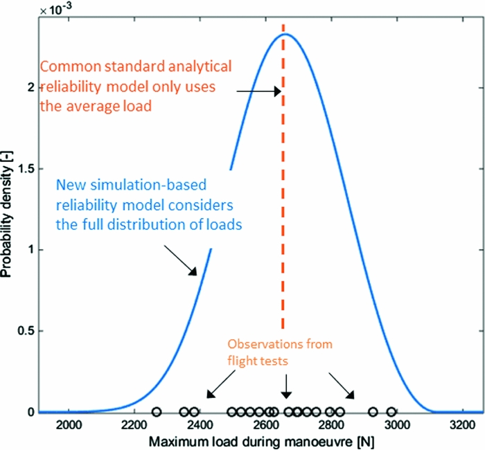
A common standard analytical method to predict a conservative fatigue life simplifies the full distribution of the loads during a flight regimeFootnote 1 to a single averaged load spectrum and only uses the average manoeuvre minimum and maximum loads to form a low-frequency Ground-Air-Ground load spectrum. Its reliability substantiation is fully derived from the distribution of component strength. Such a method thus assumes that uncertainty in flight regime loads is negligible with respect to uncertainty in fatigue strength. The validity of this assumption is, however, not obvious and may not be general. For example, flight test results in Fig. 1 clearly demonstrate significant variance in the maximum load when a lateral flight manoeuvre is repeatedly flown with a similar weight, centre-of-gravity and altitude.
Flight test observations of the maximum load on a critical component in the dynamic system when executing a lateral flight to the right under similar conditions.

This paper, therefore, introduces a new simulation-based method to predict fatigue life while also accounting for the full random distribution and uncertainty of loads.
Both methods make two core assumptions:
-
• The mission profile is known or can at least be conservatively estimated
-
• Inaccuracies in the modelling of fatigue strength, damage and accumulation are negligible
The two methodologies are applied to a simulated fatigue life prediction problem. The accuracy and applicability of the two methods will be investigated under the conditions of this synthetic problem.
2.0 ANALYTICAL FATIGUE LIFE PREDICTION
A baseline standard analytical fatigue life prediction methodology is outlined first. This analytical method is similar to the approved lifetime prediction methods for rotorcraft dynamic components applied by Airbus Helicopters Germany and to chapter 4.1 in NATO AGARD-AG-292(Reference Liard1). Section 4 later introduces a simulation-based methodology that features more complexity but aims for higher accuracy. The simulation-based method generally will make use of the same basic model for fatigue life prediction as outlined here in Sections 2.1-4.
2.1 Fatigue damage accumulation model
A fatigue damage accumulation model is needed to predict fatigue life for given component strength and loads during life. The model employed here consists of four main components: a Weibull-type S-N curve, the Goodman relation, the Palmgren-Miner linear-damage accumulation hypothesis and a specific cycle counting method.
2.1.1 S-N curve
A Weibull-type S-N curve that defines the number of load cycles until fatigue failure under constant amplitude loading:
 $$\begin{equation}
{\sigma _a}(N){|_R} = {\sigma _{{a_\infty }}} + \frac{{{\sigma _{{a_{{\rm{ult}}}}}} - {\sigma _{{a_\infty }}}}}{{{\rm{exp}}\left[ {{{\left( {\frac{{{\rm{lo}}{{\rm{g}}_{10}}N}}{{{\alpha _w}}}} \right)}^{{\beta _w}}}} \right]}},
\end{equation}$$
where σ
a
is the applied stress amplitude (at stress ratio R); N is the number of load cycles (until failure); σ
a
∞
is the stress amplitude of the endurance limit or fatigue limit (at stress ratio R); σ
a
ult
is the ultimate stress amplitude determined by:
 ${\sigma _{{a_{{\rm{ult}}}}}} = {\sigma _{{\rm{ult}}}} \times \frac{{1 - R}}{2}$
, where σult is the ultimate strength; R is the stress ratio
 $\frac{{{\sigma _{{\rm{min}}}}}}{{{\sigma _{{\rm{max}}}}}}$
; {α
w
, β
w
}are component-specific Weibull curve parameters. Alternatively, many rotorcraft manufacturers use a two-parameter exponential function to approximate an S-N function around N = 105. Although such a model is less prone to over-fitting, it generally provides over-optimistic estimates for low-cycle fatigue. A four-parameter Weibull curve, instead, can also accurately model low-cycle fatigue. A Weibull type S-N curve is expected to provide results that are more realistic when fatigue lives are simulated for very low strengths, as is done by the simulation-based model presented in Section 4 and during the Monte-Carlo simulations in Section 5.
2.1.2 Goodman-relation
The Goodman-relation to translate load cycles to the stress ratio for which the S-N curve is valid is:
 $$\begin{equation}
{\sigma _a}\left( R \right) = \frac{{{\sigma _{{a_{{\rm{ult}}}}}} \times {\sigma _a}{|_{{R_i}}}}}{{{\sigma _{{a_{{\rm{ult}}}}}} - {\sigma _m}{|_{{R_i}}} \times \frac{{1 + R}}{{1 - R}}}},
\end{equation}$$
where: σ a | Ri and σ m | Ri are the stress amplitude and mean stress of the ith load cycle class, respectively. This relation is often considered to be conservative for metallic parts, except for high-strength but low-ductility alloys, according to Schijve(Reference Schijve2).
2.1.3 Cycle counting
Rainflow counting (according to ASTM E1049-85)Footnote 2 preceded by proprietary peak-valley (PV) filtering to determine the number of cycles in each load cycle class (load spectra are discretised). Rainflow counting is generally regarded as an accurate method, e.g. Schijve(Reference Schijve2); however, other methods for cycle counting are common in industry, as well.
2.1.4 Damage accumulation hypothesis
The Palmgren-Miner linear damage accumulation hypothesis to define fatigue failure under spectrum loading is
 $$\begin{equation}
{\rm{Fatigue\ failure}} \equiv \sum {\frac{{{n_i}}}{{{N_i}}}} = 1,
\end{equation}$$
where ni is the number of load cycles in the ith load cycle class and Ni is the number of cycles until fatigue failure under constant amplitude load defined by the ith load class. This model is generally considered valid under conditions where loads are random and non-periodic. Fatigue tests under these conditions show that a damage accumulation model such as (2.3) is on average accurate, according to Schijve(Reference Schijve2).
2.2 Random strength model
As fatigue strength is a random variable, both the shape and vertical translation of an S-N curve can be considered as uncertain. While neglecting shape variations, the following random fatigue strength model is used to define an S-N-P curve:
 $$\begin{equation}
{\sigma _a}(N){|_R} = SF{|_{\hat{\sigma }}} \times \left\{ {{{\hat{\sigma }}_{{a_\infty }}} + \frac{{{{\hat{\sigma }}_{{a_{ult}}}} - {{\hat{\sigma }}_{{a_\infty }}}}}{{\exp \left[ {{{\left( {\frac{{{{\log }_{10}}N}}{{{{\hat{\alpha }}_w}}}} \right)}^{{{\hat{\beta }}_w}}}} \right]}}} \right\}
\end{equation}$$
The strength factor SF herein is a random variable distributed according to a lognormal distribution (as a transformation of an associated standard normal distribution N(0, 1)):
 $$\begin{equation}
p\left( {SF|\hat{\mu },\hat{\sigma }} \right) = {\rm{exp}}\left[ {\hat{\sigma } \times {\rm N} \left( {0,1} \right) + \hat{\mu }} \right]
\end{equation}$$
 $\{ {{{\hat{\sigma }}_{{a_{{\rm{ult}}}}}},{{\hat{\sigma }}_{{a_\infty }}},{{\hat{\alpha }}_w},{{\hat{\beta }}_w}} \}$
are Maximum Likelihood Estimates (MLEs) of the S-N curve parameters, given component static test results and/or component constant amplitude fatigue tests. The median of the strength distribution (i.e. the distribution of SF) should have its median equal to one (i.e.
 $\hat{\mu } = 0$
) such that the expected S-N curve remains unaltered. Nevertheless,
 $\hat{\mu }$
is only a sample estimate and its value can be biased and unequal to zero (i.e. offset with the true mean).
The scatter of the strength factor is assumed to be independent of N (i.e. noise is assumed to be homoscedastic). Therefore, it is allowed to translate all fatigue test results used to fit the S-N curve to an arbitrary N. A straightforward one-dimensional distribution fit can then provide
 $\hat{\sigma }$
, the MLE of the standard deviation of strength. Although the assumption of homoscedasticity does not generally hold and can be invalidated by examples where scatter positively correlates with N, e.g. Schijve(Reference Schijve2), this engineering assumption is acceptable to aviation authorities and general engineering practise in the rotorcraft industry, where scatter is often estimated in the load dimension based on test results falling in the important region around N = 105.
With the full S-N-P curve defined, a conservative working curve can be derived. For example, if a working curve should represent the fatigue strength of the (on average) weakest component out of 1 million randomly selected components, then SF work can be computed according to
 $$\begin{equation}
S{F_{{\rm{work}}}}({P_{{\rm{fail}}}} = {10^{ - 6}}) = {\rm{exp}}\left\{ {\hat{\sigma } \times {{\rm N} ^{ - 1}}\left( {0,1,{P_{{\rm{fail}}}}} \right) + \hat{\mu }} \right\},
\end{equation}$$
with N−1(0, 1, P fail) denoting the inverse Cumulative Distribution Function (CDF) of the standard normal distribution.
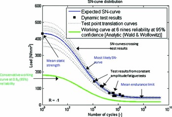
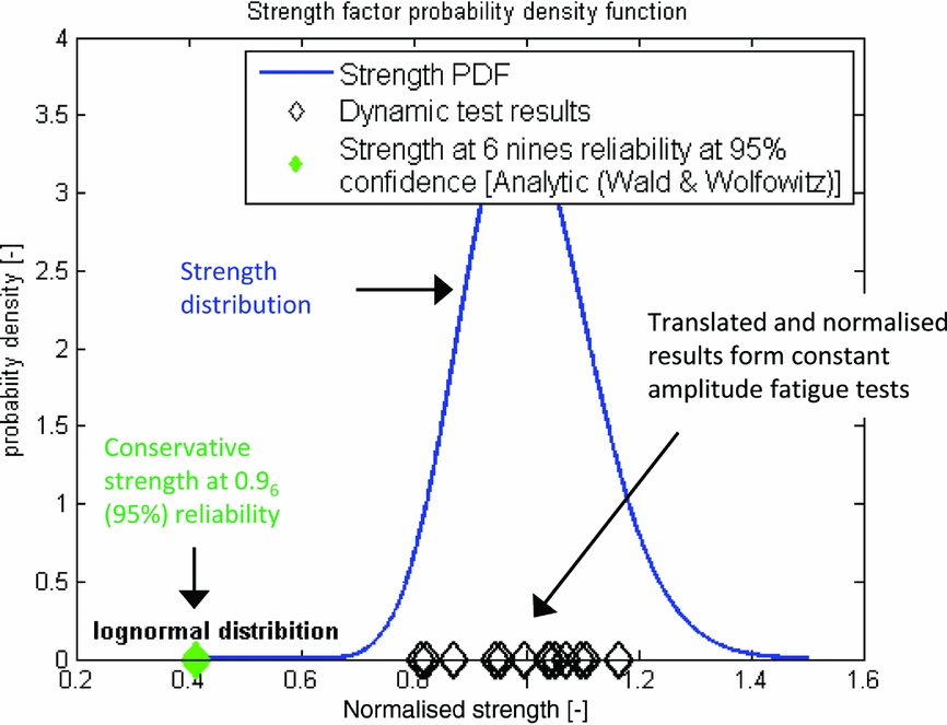
Figures 2 and 3 illustrate such a working curve.
Example of constant amplitude fatigue test results, the MLE S-N curve and conservative working curve for a component from the dynamic system.

Exemplary fatigue test results (normalised by the MLE S-N curve), the derived MLE estimate of the PDF of normalised fatigue strength (SF), and the strength factor corresponding to the conservative working curve.

Airworthiness regulations (i.e. AC 27-1B MG11) do not explicitly prescribe the use of tolerance interval analysis for fatigue life substantiation. It is common among rotorcraft manufacturers to assume that S-N relationships and associated scatter observed from large numbers of coupon tests are sufficient to make a perfect estimate of an S-N-P diagram for a specific component. Nevertheless, and according to NATO AGARD-AG-292(Reference Liard1), it is here, instead, considered that the scatter in fatigue properties of a component mainly depends on variability in tolerances, surface finishing and other properties affecting component-level manufacturing quality, and that these influences cannot be predicted accurately by coupon tests. Especially the scatter in S-N relationships must then be derived from fatigue tests of full-scale components representative for serial production.
Since only a limited number of such component-level fatigue tests can be done, it is considered to be impossible to make a perfect estimate of the S-N-P curve, especially concerning its variability. Therefore, it is considered that any estimate of the probability density function (PDF) of SF itself, and thereby also a conservative strength quantileSFwork estimated by Equation (2.6) is imperfect. To account for this uncertainty, a confidence interval for the conservative SFwork must be computed; that is, to require a 95% upper single sided confidence level here means that, if a set of fatigue tests would be repeated many times, then 95% of the conservative SFwork estimates, one for each new set of fatigue test results, would really meet a 0.999999 reliability requirement. The remaining 5% conservative SFwork estimates would, in fact, correspond to a probability of failure that would be higher than 10−6. Hahn and Meeker(Reference Hahn and Meeker3) may be referred to for further explanations on confidence intervals.
Both the mean
 $\hat{\mu }$
and standard deviation
 $\hat{\sigma }$
(of the associated normal distribution) of the strength factor SF (2.5) must thus be considered as random variables and are distributed according to(Reference Schijve2)
 $$\begin{equation}
p\left( {\hat{\mu }|\hat{\mu },\hat{\sigma },{n_{{\rm{test}}}}} \right) & =& t\left( {\mu = \hat{\mu },\sigma = \frac{{\hat{\sigma }}}{{\sqrt {{n_{{\rm{test}}}}} }},\nu = {n_{{\rm{test}}}} - 1} \right),\\
\end{equation}$$
 $$\begin{equation}
p\left( {\hat{\sigma }|\hat{\sigma },{n_{{\rm{test}}}}} \right) \propto \hat{\sigma } &\times& \sqrt {\frac{{{n_{{\rm{test}}}} - 1}}{{{\chi ^2}\left( {\nu = {n_{{\rm{test}}}} - 1} \right)}}} ,
\end{equation}$$
A conservative strength factor for the working curve at a reliability level 1 − γ (i.e. 1-10−3) and a lower single-sided confidence level α (i.e. 0.95 for 95%) can be computed by Wald and Wolfowitz(Reference Wald and Wolfowitz4):
 $$\begin{equation}
\begin{array}{l} SF\left( {\gamma ,\alpha |\hat{\mu },\hat{\sigma },{n_{{\rm{test}}}}} \right) \\[6pt] \quad = {\rm{exp}}\left\{ {\hat{\mu } - \sqrt {\frac{{{n_{{\rm{test}}}} - 1}}{{inv{\chi ^2}\left( {{P_{{\rm{fail}}}} = 1 - \alpha |\nu = {n_{{\rm{test}}}} - 1} \right)}}} \times r\left( {\gamma ,{n_{{\rm{test}}}}} \right) \times \hat{\sigma }} \right\}{\rm{,}} \end{array}
\end{equation}$$
 $$\begin{equation}
r\left( {\gamma ,{n_{{\rm{test}}}}} \right) = \frac{1}{{\sqrt {{n_{{\rm{test}}}}} }} - {{\rm N} ^{ - 1}}\left( {{P_{{\rm{fail}}}} = \gamma |\mu = 0,\sigma = 1} \right)
\end{equation}$$
2.3 Load model
The loads during a service life are represented by a load spectrum that is cycle counted from a load sequence. Ideally, this load sequence would be the continuous load signal measured on the component during its life. In practise though, a conservatively estimated load spectrum is used instead.
The first step in obtaining this load spectrum is to define a set of manoeuvres that cover how the helicopter can be flown. For example, A: take-off; B: level flight; C: hover; etc. Using these regimes, a mission profile can be made. This mission profile sets how much time, as a percentage, the helicopter spends in each manoeuvre, e.g. [A: 3%; B: 80%; . . .], and in which sequence the manoeuvres are flown per unit of time, e.g. [A C B F B . . .] every 100 flight hours (FH).
In practise, this mission profile is generally based on pilot and operator surveys as well as experience. In any case, it must be conservative for all helicopters in the fleet for which fatigue life is predicted.
Test flights with a specially instrumented helicopter may, in practise, provide continuous recordings of component loads during the manoeuvres. The same flight regimes are generally flown multiple times to, for example, cover variations in manoeuvre execution.
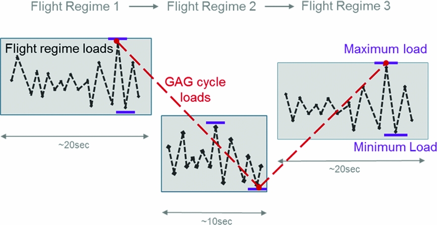
The fatigue damage that is accumulated during a flight is computed with a load spectrum of the type, as in Fig. 4. The total fatigue relevant load spectrum for a flight is thus the summation of the load spectra of each flight regime and the load spectrum from the Ground-Air-Ground (GAG) load sequence. The GAG load sequence accounts for the transitions between the manoeuvres and is the most severe load signal that goes through the extreme (i.e. minimum or maximum) load in each manoeuvre.
Flight regime loads and GAG loads. These loads together make out the full load spectrum.

There is uncertainty regarding manoeuvre loads and manoeuvre extreme loads when predicting the loads during the full fatigue life. In case of manoeuvre loads, the measured load spectra, one for each time the flight regime was flown during test flights, are averaged and scaled by linear weighting to a reference time (i.e. 100FH). Extreme loads from multiple manoeuvre load tests are simply averaged. Inserting these averaged loads into the conservative mission profile and according to the model in Fig. 4, leads to an average load spectrum per unit of time.
2.4 Perfect modelling assumption
Throughout all analysis, it is assumed that the outlined models for fatigue damage accumulation, random fatigue strength and loads are perfect (i.e. do not introduce any errors or additional uncertainties). This is in line with standard practise in rotorcraft industry and in compliance with AC 27-1B MG11. Nevertheless, different manufacturers generally make use of different models and design assumptions to comply with airworthiness regulations. Everett(Reference Everett5) observed that fatigue life predictions by different manufacturers for the same component can vary significantly. The accuracy and precision tests conducted in Section 5, therefore, have a limited scope, as they also incorporate the assumption of perfect modelling. Modifying or removing one or more of the adopted modelling assumptions may significantly alter the outcome of the analysis.
2.5 Substantiated fatigue life prediction
Commonly, a Service Life Limit (SLL) is set according to a maximum allowed probability of fatigue failure during the service life (e.g. P fail(SLL) = 10−6). However, most general safety analysis works with reliability requirements expressed as a probability of failure per flight hour and not per service life.
When it must be substantiated that the probability of failure in a next flight hour will on average never exceed a required P fail, for example 10−9, and when this requirement is not specified while assuming a constant failure rate, then the SLL follows from the following optimisation problem:
 $$\begin{equation}
SLL = \mathop {{\rm{arg}}\;{\rm{min}}}\limits_{\left\{ {l \in \mathbb{R}:L > 0} \right\}} {\left( {{P_{{\rm{fai}}{{\rm{l}}_{nextFH}}}}(l) - {\gamma _{FH}}} \right)^2},
\end{equation}$$
where γ FH is the maximum allowed average probability of failure per flight hour and P fail nextFH (l) denotes the average probability of failure during the next flight hour after l flight hours have been accumulated. P fail nextFH (l) can be computed using the SLL reliability estimator P fail(SLL):
 $$\begin{equation}
{P_{{\rm{fai}}{{\rm{l}}_{nextFH}}}}\left( l \right) = \frac{{{P_{{\rm{fail}}}}\left( {l + 1} \right) - {P_{{\rm{fail}}}}\left( l \right)}}{{1 - {P_{{\rm{fail}}}}\left( l \right)}}
\end{equation}$$
For simplicity, this work will only further consider the reliability estimator P fail(SLL) i.e. the estimator of a probability of failure per service life.
In either case and in line with AGARD-AG-292(Reference Liard1), the analytical method assumes that the reliability of a working curve can only substantiate overall reliability e.g. the standard analytical method substantiates an SLL with a probability of failure of 10−6/life at a 95% single-sided upper confidence level by:
-
• a working curve with γ = 10−6 and α = 0.95 in(2.9).
-
• a load spectrum according to a conservative mission profile and average manoeuvre (extreme) loads.
There is no reliability derived from the conservative mission profile. The reliability requirement must be met for all helicopters and for all flight hours. If the conservatism that is incorporated in the conservatively estimated design mission profile would be used to substantiate additional reliability, then this would only be valid for, at most, averagely demanding operators; that is, this additional reliability would apply to VIP operators but significantly less to Search and Rescue operators.
3.0 STATE-OF-THE-ART IN PROBABILISTIC FATIGUE LIFE PREDICTION
Questions have been raised during the last decades on the accuracy of the reliability substantiation in standard fatigue life predictions, for example by Lombardo and Fraser(Reference Lombardo and Fraser6). They specifically drew attention to uncertainties coming from mission profile and design load spectrum estimation but also to possible inaccuracies in standard models used to estimate fatigue damage (e.g. the Palmgren-Miner linear accumulation hypothesis). To the best of the authors’ knowledge, there has so far been no systematic attempt to develop numerical error models for such standard fatigue damage models. This is also outside the scope of this analysis. The influence of uncertainties from the estimation of regime loads and design load spectra on predicted fatigue life has, however, been researched before.
Thompson and Adams(Reference Thompson and Adams7) were one of the first in the rotorcraft industry to extensively model the reliability of SLLs. They included the combined uncertainty from variance in component strength, regime loads and mission profiles in a reliability substantiation model by using a Basic Monte Carlo (BMC) simulation and models for random strength, loads and usage. For their random load model, the average load spectrum per manoeuvre and also the statistical distribution of manoeuvre maximum loads was computed from results of dedicated flight tests. The manoeuvre load spectrum was assumed linearly proportional to the random manoeuvre maximum load; that is, when a maximum load is drawn that is twice the average, the corresponding spectrum is the average spectrum but with the number of cycles multiplied by two. Not accounting for GAG loads and assuming that helicopters randomly change mission profile every 103FH, the percentage of time spent in each manoeuvre is set as a random variable, as well (based on extensive usage data). Their (random) strength model was similar to the model in Section 2.2. Due to the low efficiency of BMC for aerospace-typical low-failure probabilities, it was necessary to estimate these probabilities by tail extrapolation of a distribution fit through a limited number of BMC samples.
This work was extended by Zhao and Adams(Reference Zhao8,Reference Zhao and Adams9) , where use was made of importance sampling, preceded by First- and Second-Order Reliability Modelling (FORM/SORM) to first estimate the critical failure region in the parameter space.
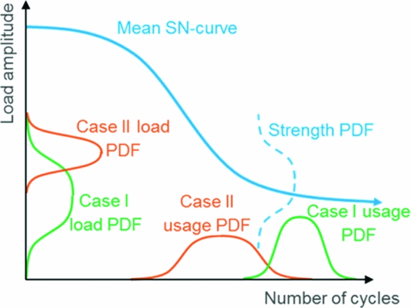
Benton(Reference Benton10) and others(Reference Tang and Zhao11–Reference Brown and Chang14) have all introduced (semi-) analytical fatigue life reliability substantiation models. Each of these requires specifying a PDF for the amplitude and number of cycles of every load case to be considered, i.e. defined as a constant amplitude loading block, and also made use of a random strength model similar to Section 2.2. This framework is displayed in Fig. 5.
Schematic of the random model framework for recent (semi-)analytical SLL reliability models (shown with two load cases).

All previous work on reliability substantiation for fatigue life prediction confirmed the importance and value of explicit and combined modelling of uncertainty in strength, loads and usage. Thompson and Adams used their work to re-confirm their standard fatigue life design methodology. However, Tong et al(Reference Tong, Antoniou and Wang15) have challenged the accuracy of the method presented by Thompson and Adams and argue that the conservative treatment of loads by Thompson and Adams does not add significant reliability to the overall fatigue life prediction. The results from Tong et al encourage the assumption that all reliability may be substantiated by a conservative working curve, as employed by the simplified analytical method in Section 2.2. In addition, their results demonstrate that the assumption by Thompson and Adams that sources of reliability can be linearly added may not hold.
The following challenges were identified based on previous work:
-
• It is difficult to model situations of complex spectrum loading, i.e.as in Fig. 4, in the framework of current (semi-)analytical methods (i.e. as in Fig. 5).
-
• The manoeuvre load model of Thompson and Adams effectively bounds the maximum spectrum load to the highest load measured in test flights. In practise, however, it is observed that the extreme load during a manoeuvre can be considered as an unbounded random variable. Due to the non-linearity of the S-N curve, PV filtering and range counting, it is expected that only scaling of the number of cycles in a reference spectrum will generally, not accurately, reflect random variations in manoeuvre damage. For example, even when considering a spectrum with only one cycle, then doubling the maximum load of this cycle, can have a significantly different effect on manoeuvre damage than doubling the count of this cycle.
-
• None of the previous work includes tolerance intervals (i.e. confidence intervals on quantiles) despite the high uncertainty associated with probabilistic fatigue life predictions derived from few statistical samples, as is common in rotorcraft industry.
4.0 SIMULATION-BASED SUBSTANTIATION
A new simulation-based methodology to substantiate fatigue life predictions for critical components in the helicopter dynamic system is presented. This new method aims to meet the following main requirements:
-
• Model combined uncertainty from loads and strength
-
• Be applicable to problems of very high dimension (i.e. mission profiles with many flight regimes)
-
• Be suitable up to very low failure probabilities (i.e. 10−9)
-
• Improve accuracy and generality with respect to previously introduced models
-
• Provide tolerance intervals
-
• Feature reasonable computational costs
4.1 Modelling assumptions
The following fundamental assumptions are made in the development of this model:
-
• Perfect fatigue modelling, see also Section 2.4
-
• Helicopters’ mission profile is known or can be conservatively assumed and can be modelled as in Section 2.3
-
• Flight regime loads are independent. For example, an abnormally high load in a turn to the left is uncorrelated to the load in a next right turn
The practical implementation of the model also assumes that regime loads are identical throughout a fatigue life (e.g. all turns are flown identically). This practical assumption is expected to promote variance in lifetime and thus to be conservative (i.e. loads do not average-out during life). This feature can, however, easily be lifted and is not a necessary condition for practical use of the proposed model. This is important, as it may also be argued that a small change in a single load can have a major effect on fatigue life due to the non-linearity of the S-N curve. The presence of a single high load ‘outlier’ may then have a dominating effect on fatigue life. Then, it would be reasonable to conclude that the rate of occurrence of a high load ‘outlier’ may be too restricted if loads are only sampled once for each manoeuvre type, instead of once per occurrence of the manoeuvre.
4.2 Modelling of random variables
The substantiation model features an independent probabilistic strength model and a strength-dependent combined probabilistic manoeuvre load and fatigue damage model which is similar to the model used by the virtual fatigue damage accumulation sensor from Dekker et al(Reference Dekker, Bendisch and Hoffmann16).
4.2.1 Stochastic fatigue strength model
The implemented random fatigue strength model is equal to Section 2.2. Note, that as the proposed substantiation model is simulation-based, the new methodology may easily be adapted to accommodate other strength models.
4.2.2 Stochastic load spectrum model
Ideally, flight regime loads can be modelled in full and with only a small number of random parameters e.g. by means of Fourier decomposition and/or Principle Component Analysis. It was observed that, especially in complex and dynamic manoeuvres, the high frequency content of load signals is most relevant for fatigue damage modelling. Unfortunately, there is often not enough flight data available to reliably derive the high number of model parameters that would be necessary to properly represent these high frequency load signal features.
Instead, it was found that modelling of fatigue damage that is equivalent to the full load signal during a flight regime is easier than attempting to model the full load signal. Distribution fits through available test flight data, and large samples with synthetically generated flight manoeuvre load sequences demonstrated that, for a given S-N curve, and given that there is at least one half-cycle above the endurance limit, the flight regime fatigue damage follows a generalised extreme value (GEV) distribution.
The GEV distribution of a parameter x is defined as follows:
 $$\begin{equation}
\begin{array}{l} {\rm{if }}\;k \ne 0\ {\rm{ then{:}}}\\[3pt] p\left( {x|k,\mu ,\sigma } \right) = \frac{1}{\sigma }{\rm{exp}}\left[ { - {{\left( {1 + k\frac{{x - \mu }}{\sigma }} \right)}^{ - \frac{1}{k}}}} \right]{\left( {1 + k\frac{{x - \mu }}{\sigma }} \right)^{ - 1 - \frac{1}{k}}},\\[3pt] {\rm{else{:}}}\\[4pt] p\left( {x|k,\mu ,\sigma } \right) = \frac{1}{\sigma }{\rm{exp}}\left[ { - {\rm{exp}}\left( { - \frac{{x - \mu }}{\sigma }} \right) - \frac{{x - \mu }}{\sigma }} \right]{\rm{ }} \end{array}
\end{equation}$$
where [k, μ, σ] are distribution parameters.
The magnitude of the minimum and maximum load that occurs within a flight regime is also described by a GEV distribution. Again, distribution fits through large samples with synthetically generated manoeuvre load sequences, but, as well as through available test flight data, are in agreement with this choice.
A random model that represents the load model, as in Fig. 4, can now be established for a given fatigue strength by defining for each manoeuvre:
-
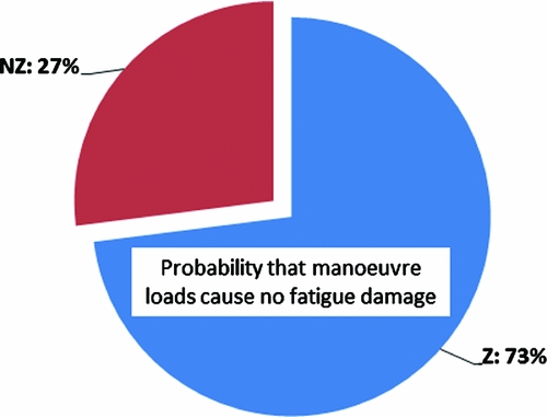
• The probability that load cycles within the flight manoeuvre cause fatigue damage. This can be estimated by computing the fatigue damage for each available manoeuvre loading sample and by computing the ratio between the number of times the manoeuvre was flown with and without causing damage. A visualisation of a resulting binomial distribution is shown in Fig. 6. This feature circumvents a discontinuity in the manoeuvre damage distribution. Due to the endurance limit, many manoeuvre instances may not cause any manoeuvre damage at all, whereas the damage of the damaging instances is GEV distributed.
-
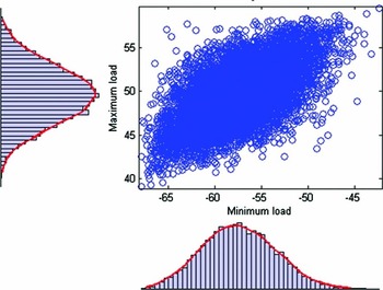
• If there is no regime damage, a multivariate probability density functions for the minimum and maximum load during the manoeuvre. Such a distribution is shown in Fig. 7.
-
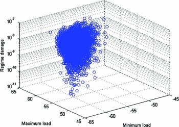
• If there is manoeuvre damage, a multivariate PDF for manoeuvre damage and extreme loads. Figure 8 shows an example of such a distribution.
Pie chart showing how probable it is that there are load cycles within a particular flight regime above the endurance limit (Z) or not (NZ).

A large sample from a fitted multivariate manoeuvre minimum and maximum load distribution (i.e. manoeuvre damage is zero). The corresponding marginal distributions are also shown.

A large sample from a fitted multivariate manoeuvre damage and extreme load distribution.

The multivariate distributions in the practical implementation of the model are realised by t-copulas(Reference Genest and Favre17). An alternative implementationFootnote 3 by means of NATAF transformation (Hurtado(Reference Hurtado18)) resulted in non-conservatively biased and inaccurate results according to an idealised and synthetic verification test. (The method of this verification test will be detailed in Section 5.2.2; a true probability of the failure of 10−3 was over-optimistically estimated as 5.9 × 10⁻⁴, whereas using t-copulas resulted in a virtually error-free estimate). Following the work of Lebrun and Dutfoy(Reference Lebrun and Dutfoy19), NATAF's limitations in modelling (tail) dependence of correlated multivariate distributions may provide an explanation.
4.3 Review of reliability estimation methods
The reliability of an SLL is one minus the probability that a component experiences a fatigue failure before it reaches the SLL:
 $$\begin{equation}
R\left( {{\rm{SLL}}} \right) = 1 - {P_{{\rm{fail}}}}\left( {{\rm{SLL}}} \right)\quad {\rm{with}}\quad {\rm{failure}} \equiv L < {\mathop{\rm SLL}\nolimits}
\end{equation}$$
Considering that the fatigue life L of a specific component is a function of the random parameter vector ω (i.e. containing the sampled strength factor and sampled loads and damages of the manoeuvres), the following indicator function I(. . .) can be defined:
 $$\begin{equation}
{\rm I} \left[ {L\left( \omega \right)} \right] = \left\{ {\begin{array}{*{20}{l@{\quad}}} {1\quad{\rm{ if }}L\left( \omega \right) < {\rm{SLL }}}\\ {0\quad{\rm{ otherwise }}} \end{array}} \right.
\end{equation}$$
Analytically, P fail can now be computed as:
 $$\begin{equation}
{P_{{\rm{fail}}}}({\rm{SLL}}) = \int\limits_\Omega {{\rm I} \left[ {L\left( \omega \right)|{\rm{SLL}}} \right] \times p\left( \omega \right) \times d\omega }
\end{equation}$$
However, such an integral over the parameter space Ω is not expected to be mathematically tractable for the model in Section 4.2.
4.3.1 Practical numerical reliability estimators
The most intuitive way to estimate P fail(SLL) is by a BMC estimator:
 $$\begin{equation}
{P_{{\rm{fail}}}}\left( {{\rm{SLL}}} \right) = \frac{1}{{{n_{{\rm{sim}}}}}}\sum\limits_{i = 1}^{{n_{{\rm{sim}}}}} {\left\{ {{\rm I} \left[ {L\left( {{\omega _i}} \right)|{\rm{SLL}}} \right]} \right\}} \quad {\rm{as}}\quad {n_{{\rm{sim}}}} \to \infty ,
\end{equation}$$
which is simply drawing a large number, nsim , of parameter vectors from the parameter PDF p(ω), computing the corresponding fatigue lives and then the fraction of parameter vectors that produce a fatigue life lower than the SLL.
The coefficient of variation (CoV) of a BMC estimate of P fail approximately approaches:
 $$\begin{equation}
Co{V_{{P_{{\rm{fail}}}}}} = \frac{{{\sigma _{{P_{{\rm{fail}}}}}}}}{{{\mu _{{P_{{\rm{fail}}}}}}}} = \sqrt {\frac{{1 - {P_{{\rm{fail}}}}}}{{{P_{{\rm{fail}}}} \times {n_{{\rm{sim}}}}}}}
\end{equation}$$
The estimation error is thus proportional to
 $1/\sqrt {{n_{{\rm{sim}}}}} $
and independent of the dimension of Ω. This is a highly advantageous feature, as the dimension of the parameter vector according to the model in Section 4.2 is generally high. However, when the precision of the estimate needs to have a CoV of 30%, then it is required to evaluate approximately 10/P
fail BMC samples. This means that estimating an aerospace-typical small P
fail becomes highly impractical due to the very large number of samples that need to be evaluated.
Traditionally, reliability problems have been solved semi-analytically by First- and Second-Order Reliability Methods(Reference Hurtado18). These methods are, however, only accurate under strict conditions, require transformation of the parameter space to a multivariate standard normal distribution (e.g. by transformation of the marginal distributions into Gaussians and by NATAF transformation), and their computational costs are strongly dependent on the dimension of Ω. Utilisation of FORM/SORM to handle the high-dimensional and potentially discontinuous parameter space that the model in Section 4.2 stipulates was probedFootnote 4 but did not yield encouraging results and was abandoned.
Importance Sampling(Reference Hurtado18) is another common technique to improve the efficiency of the BMC estimator. However, this requires defining a special sampling distribution around the critical region i.e. where L(ω) ≈ SLL, which is commonly obtained following FORM/SORM solutions. Improperly setting this special sampling distribution may cause large errors in the estimate of P fail. The model in Section 4.2 dictates a high dimension and complexity of the parameter space. Setting a proper sampling distribution is thus difficult, even more so given the discouraging results from FORM/SORM for the simulation-based model. Therefore, importance sampling was not pursued as a solution method.
Most other studied methods, such as BMC acceleration by statistically ‘learned’ indicator functions, e.g. by Kriging(Reference Echard, Gayton and Lemaire20) or Support Vector Machines(Reference Hurtado18), or recent Particle Algorithms(Reference Caron, Guyader, Zuniga and Tuffin21) were also considered unappealing for the particular problem at hand, mainly due to their complexity and difficulties due to the high dimensionality and the complexity of Ω that the model in Section 4.2 dictates.
4.3.2 Subset simulation
The method of choice that is implemented to estimate P fail is subset simulation (SS) as developed by Au and Beck(Reference Siu-Kui and Beck22). The core concept is to divide a difficult problem of estimating a total probability of failure into multiple sub-problems that are, by themselves, easy to solve. Considering the CoV of the BMC estimator (4.6), it shows that estimating, for example, a 1/10 probability of failure, can be done with reasonable accuracy while using ‘only’ 100 samples, independent of the dimension of the parameter space. SS exploits this benefit by estimating the total probability of failure by multiplication of a sequence of conditional high failure probabilities.
A set of intermediate failure events can be defined such that:
 $$\begin{equation}
{F_1} \supset {F_2} \supset ... \supset {F_m} = F
\end{equation}$$
This means that the failure event Fm ≡ L < SLL m is a subset of the more probable intermediate failure event F m−1 ≡ L < SLL m−1, which is, in turn, a subset of the even more probable intermediate failure event F m−2 ≡ L < SLL m−2, and so forth.
The total probability of failure is now:
 $$\begin{equation}
{P_{{\rm{fail}}}} = {P_{{\rm{fail}},}}_1 \times \prod\limits_{j = 2}^m {{{\left. {{P_{{\rm{fail}},j}}} \right|}_{{F_{j - 1}}}}}
\end{equation}$$
Here, P fail,1 is the probability of the first intermediate failure event F1 . And P fail, j | F j−1 is the probability of failure event Fj, , given that the more probable failure event Fj-1 occurs.
Computation of P fail ,1 can be done straightforwardly by a BMC estimator, especially when the first intermediate failure event F1 is set such that P fail ,1 equals an easy to compute probability γ (i.e. 1/10). Now, a limited number of samples are drawn (i.e. 100), and the fatigue life is predicted for each of these samples. The intermediate failure event F1 is then defined such that P(SLL1 > L) = γ. For example, the first intermediate limit state SLL1, or intermediate failure boundary, an implicit hyper-surface in Ω, is set such that 10 out of 100 of the initial samples lie in the first intermediate failure domain.
A similar procedure can be followed for the subsequent intermediate failure events. Again making use of a simple BMC estimator, it is now, however, necessary to generate samples that are part of the intermediate failure domain Fj-1 . Generation of a random sample that is conditional on the domain Fj-1 can be done with Modified Metropolis Hastings Markov Chain Sampling, see Ref. 19 for a detailed description.
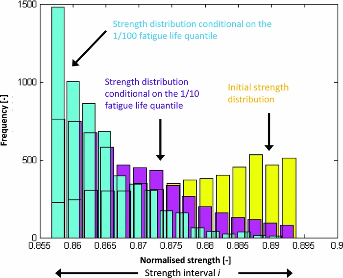
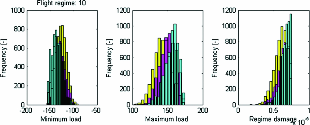
Additional intermediate failure events are added until the actual SLL for which P fail needs to be known is reached. Figures 9–11 show an example of computing P fail(SLL, si ) by subset simulation.
Example of SS, where it takes three intermediate failure events (black stars) to reach the SLL under evaluation (red diamond). The initial lifetime sample is in yellow, the lifetime distribution conditional on F1 is purple and the lifetime distribution conditional on F2 is light blue.P fail(SLL, si ) ≈ 0.1 × 0.1 × 0.2 = 0.002.

Strength samples from SS from the example in Fig. 4.4. Note that the strength generally decreases as the intermediate failure events become less probable.

SS samples of the minimum load, maximum load and regime damage of a flight regime from the example in Fig. 4.4. Note that the maximum load in the middle graph generally increases with less likely intermediate failure events, as would be expected.

4.4 Estimating the reliability of an SLL
The load model from Section 4.2.2 causes that the PDFs for regime damage and extreme load are dependent on the fatigue strength, which is itself a random variable. Therefore, P fail should be computed according to:
 $$\begin{equation}
{P_{{\rm{fail}}}}\left( {{\rm{SLL}}} \right) = \int {{p_{{\rm{fail}}}}\left( {{\rm{SLL}},s} \right) \times p\left( s \right) \times ds} \approx \sum\limits_i^{{n_{{\rm{bin}}}}} {\left[ {{P_{{\rm{fail}}}}\left( {{\rm{SLL}},{s_i}} \right) \times P\left( {{s_i}} \right)} \right]}
\end{equation}$$
The discretised integral is evaluated by discretising the strength distribution into i intervals (bins) and while assuming that, within each strength interval:
-
• Regime damage is constant and according to the lowest strength value in the interval
-
• Correlations between regime extreme loads (and regime damage) are invariant
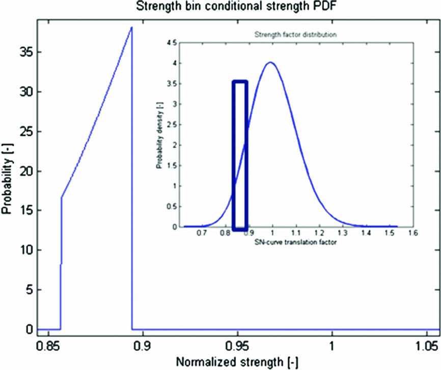
The parameter PDFs are now fixed for each strength interval. The strength PDF in one such interval is as in Fig. 12. Note that, in general, the coarser the strength discretisation grid, the more conservative the estimates of P fail, as regime damage is consistently overestimated. This was confirmed by simulations under both ideal and small sample size conditions. High imprecision may arise, though, if too few samples per subset are used in combination with a very coarse strength grid.
Example of strength PDF that is conditional on a strength interval, here in the upper right thick blue box.

4.5 Confidence interval on SLL reliability
In practise, the number of fatigue tests and flight tests that can be done is limited. Also, computational resources are generally limited so that the sample sizes used in SS must be limited. This means that both the parameter distributions themselves, as well as computational results from the quantile estimator (4.8), are actually subject to significant uncertainty. It is assumed that other sources of uncertainty (i.e. establishing of the copulas) can be neglected or are conservatively hedged.
Confidence intervals on P fail are computed by parametric and non-parametric bootstrapping(Reference Hesterberg, Moore, Monaghan, Clipson and Epstein23). Essentially, this means that P fail is computed for several alternative variants of the strength, regime extreme load and regime damage distributions, and for several alternative SS estimates. Thus, a distribution for P fail can be estimated and, for example, the upper 95th percentile of P fail can be selected for an upper single sided 95% confidence interval. An example is shown in Fig. 13.
Example of the PDFs of bootstrap estimates of P fail(SLL). The width of a PDF represents uncertainty due to limited SS accuracy, and the variance in the mean of the different PDFs represents uncertainty due to a low number of fatigue and manoeuvre load tests. It demonstrates that imprecision from SS is small with respect to uncertainty due to a low number of fatigue and manoeuvre load tests. The result was obtained for seven available fatigue tests and 15 instances per manoeuvre.

Au and Beck(Reference Siu-Kui and Beck22) provide an algorithm to estimate the coefficient of variation CoV P fail, i for P fail(SLL,si ) in (4.9), while assuming that P fail(SLL,si ) is normally distributed. The standard deviation of P fail can then be estimated as:
 $$\begin{equation}
{\hat{\sigma }_{{P_{{\rm{fail}}}}}} = \sqrt {\sum\limits_i^{{n_{{\rm{bin}}}}} {{{\left[ {Co{V_{{P_{{\rm{fail}}}},i}} \times {P_{{\rm{fail}}}}\left( {{\rm{SLL,}}{s_i}} \right) \times P\left( {{s_i}} \right)} \right]}^2}} }
\end{equation}$$
This feature is important as it allows using small sample sizes in SS (i.e. for low computational costs) while still ensuring conservatism.
Alternative regime loads are determined by non-parametric bootstrapping (i.e. random ‘reshuffling’ with allowing duplicates) of the available manoeuvre load tests results. Note that standard literature indicates that non-parametric bootstrapping is inaccurate and generally not conservative for small sample sizes. This was also confirmed by extensive simulations by the authors. Nevertheless, it is assumed that this inaccuracy is negligible (i.e. small in comparison to variance due to parametric bootstrapping of the estimated strength distribution). Previous sensitivity studies (e.g. by Zhao and Adams) show that fatigue strength is significantly more influential than manoeuvre loads in fatigue life prediction and thereby support this assumption.
Alternative strength factor distributions are simply drawn from the parameter PDFs (2.7) and (2.8). This method of parametric bootstrapping was confirmed to be accurate by means of extensive simulations by the authors.
5.0 VALIDATION OF SUBSTANTIATION MODELS
5.1 Synthetic reference problem
Straightforward validation on a real fatigue life prediction case is fundamentally impossible due to the extremely large sample sizes that would be required, e.g. to define a real fatigue life distribution. It would imply flying a very large number (>>103) of helicopters under an identical mission profile until (catastrophic) fatigue failure of the component under investigation has occurred on all machines. Therefore, the analytical and simulation-based fatigue life prediction substantiation models are both tested only on a synthetic reference problem for which the ‘true’ fatigue life distribution can be simulated. This reference case is designed to be realistic but is not specific for any particular helicopter component.
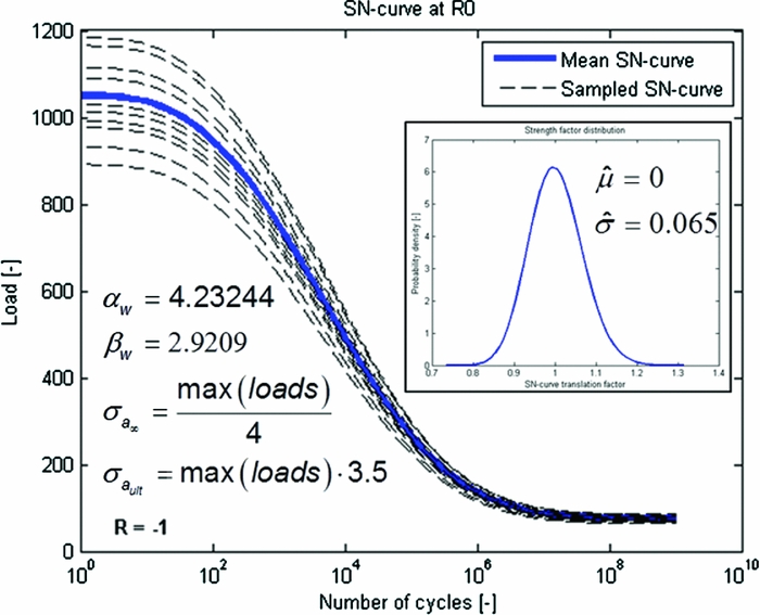
The definition of the S-N-P curve is as in Fig. 14. The standard deviation of the strength factor is set to a realistically low value to maximise the relative influence of variance in loads on fatigue life. This is important as the simulation-based model is meant to improve accuracy by explicitly accounting for the influence of uncertainty in loads on fatigue life.
Definition of the S-N-P curve in the reference problem. See also Equations (2.1) and (2.5). ‘Loads’ refers to all sampled load signals, as in Fig. 15.

Random synthetic flight regimes are used to doing ‘virtual manoeuvre load testing.’ A Fourier series is used to form a random load signal for the ith synthetic regime of the ith virtual manoeuvre load test:
 $$\begin{equation}
{{\rm{[Load\ signal]}}_i}{\rm{ }} = \sum\limits_{n = 1}^k {{a_{i,n}}{\rm{Sin}}({f_{i,n}} \times {t_F} + {\phi _{i,n}}) + {m_{i,n}}} ,
\end{equation}$$
where tF is a synthetic time vector discretising the domain [0, 2π] into 150 points, and where {a, f, ϕ, m} are randomly drawn load signal parameters defining an ordinary Fourier series.
For each manoeuvre, random manoeuvre-type parameters set a multivariate distribution from which the load signal parameters are drawn. K = 5 signal parameters are randomly drawn from the distributions that these random manoeuvre-type parameters define, each time a virtual manoeuvre load test is performed:
 $$\begin{equation}
[ {{a_i},{f_i},{\phi _i},{m_i}} ] = {\rm N} ( {[ {{\mu _{a,i}},{\mu _{f,i}},{\mu _{\phi ,\iota }},{\mu _{m,i}}} ],[ {{\sigma _{a,i}},{\sigma _{f,i}},{\sigma _{\phi ,\iota }},{\sigma _{m,i}}} ]} )
\end{equation}$$
To define the virtual flight manoeuvres, the manoeuvre type parameters for i = 15 different manoeuvres are randomly drawn from the following uniform and/or normal distributions:
 $$\begin{equation}
\begin{array}{*{20}{l@{\quad}}} {{\mu _m} = U\left[ { - 10,10} \right] \times 2.7}&{{\sigma _m} = {\rm N} \left( {0,1} \right) \times 1.4}\\ {{\mu _f} = {\rm N} \left( {0,1} \right) \times 45{\rm{ }}}&{{\sigma _f} = {\rm N} \left( {0,1} \right) \times 1.5}\\ {{\mu _a} = {\rm N} \left( {0,1} \right) \times 45{\rm{ }}}&{{\sigma _a} = {\rm N} \left( {0,1} \right) \times 0.4}\\ {{\mu _\phi } = {\rm N} \left( {0,1} \right) \times 0.2 \times \pi {\rm{ }}}&{{\sigma _\phi } = {\rm N} \left( {0,1} \right) \times 1.2}, \end{array}
\end{equation}$$
where the scaling factors were set by the tuning of the synthetic reference problem such that it is representative and realistic. Changing the parameters in (5.3) can be used to change the nature of the load spectra occurring in the synthetic reference problem.
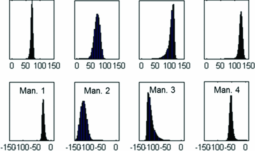
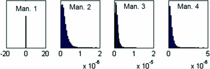
Some load signals generated by the random flight regime model are shown in Fig. 15. Corresponding distributions for regime minimum and maximum load are given in Fig. 16. Figure 17, then, shows corresponding regime damage distributions, computed with strength factors according to the distribution defined in Fig. 14.
Example of artificially generated test flight data. Note the similarity between samples for the same regime and the difference between the regimes.

Example of reference flight regime maximum (above) and minimum (below) load (marginal) distributions.

Example of reference flight regime damage (marginal) distributions.

The mission profile is randomly defined by drawing a random sequence of 150 flight regimes and setting the regime timeshare proportional to the number of occurrences of the regime in the random sequence. Figure 18 shows an example of a drawn sequence of manoeuvre extreme loads.
Example of sampled GAG extreme manoeuvre loads before extreme load and Peak Valley filtering.

Defining a reference problem in this way allows doing a virtually infinite number of flight and fatigue tests. For a randomly generated problem, it is thus possible to very accurately simulate the ‘true’ distribution of fatigue life by simple BMC simulation. Figure 20 shows such a reference fatigue life distribution. All the reference distributions that are used for validation contain 105 samples. The CoV of the ‘true’ P fail of the ‘true’ 10−3 lifetime quantile is then 10%, according to Equation (4.6). This means that it is roughly 99.7% certain that the P fail of the ‘true’ 10−3 lifetime quantile is actually between 1.3 × 10⁻³ and 0.7 × 10⁻³. This imprecision must be considered when regarding observed estimation errors of the models.
The 10−3 quantile of the ‘true’ lifetime distribution can thus be estimated with high precision by BMC simulation and without making any assumptions about the distribution of fatigue life. However, tests for estimating a more realistic 10−6 quantile can only be conducted when the distribution of the ‘true’ reference sample of size 105 is extrapolated. To do this, it is assumed that fatigue life follows a GEV distribution. Although GEV distribution models generally fit simulated lifetime distributions very well, cases have been observed where the fit appeared to model the lower tail too conservatively, potentially leading to the presentation of (slightly) over-conservative test results in this work. The use of dedicated tail modelling may remediate this inaccuracy in future work.
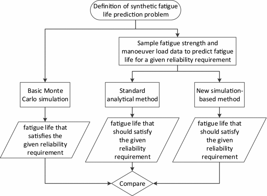
Such ‘true’ reference distributions of fatigue life are used to validate the analytical and simulation-based methods (see also Fig. 19).
Overview of the validation procedure to test the reliability of the analytical and simulation-based fatigue life prediction methods.

5.2 Verification test under idealised circumstances
First, the ideal performance of the standard analytical (Section 2) and new simulation-based (Section 4) fatigue life substantiation models are tested to see if these models are asymptotically correct. Ideal conditions are defined as having 5 × 10⁵ fatigue tests and 104 flight tests availableFootnote 5 . Hence, if a model makes wrong estimates, then this must be due to fundamental shortcomings in the model itself, as there is practically no uncertainty in the fitted strength and load distributions that serve as input to the models.
5.2.1 Standard analytical method
The standard method is tested by using the ‘true’ lifetime distribution to compute the actual P fail of the lifetime quantile that the standard method predicts. As in Fig. 20, this actual P fail is about 7 × 10⁻³ (i.e. the failure probability of the predicted lifetime is about seven times higher than the target of 10−3). A repetition of the test, while instead targeting a more realistic and challenging 10−6 lifetime quantile, also led to a non-conservatively biased ‘true’ fatigue life quantile of about 5.9 × 10⁻⁵. These results indicate that the standard reliability substantiation model is, under ideal circumstances, inaccurate and non-conservative. The cause is that the standard method only computes with the average (extreme) loads and neglects effects of their variance.
Comparison between the (synthetic) 10−3 lifetime quantile according to the reference distribution and the standard prediction method.

5.2.2 Simulation-based method
The new simulation-based fatigue life substantiation model is tested differently, as it does not directly predict a lifetime quantile. It is only tested if the new model indeed predicts a 10−3 probability of failure for the lifetime that is already known to be the 10−3 quantile of the ‘true’ reference lifetime distribution.
The test result is depicted in Fig. 21. The circles in the blue line show P fail(SLLref) for the ith strength interval. The probability of having a component in the ith strength interval is displayed by the squared red line. The triangulated black line shows the point-wise multiplication between P fail(SSL,s i), given strength and the probability of this given strength. The dotted green line finally shows the cumulative probability of failure, which here accumulates to 1.05 × 10⁻³. The P fail(SSL,s i)estimates are made for sequentially increasing strength intervals, starting at the lower tail. When these probability estimates become very small, and as soon as the product of the ith estimated probability of failure and the probability of a strength value in the ith interval itself no longer provides a significant contribution to the overall reliability integral (4.9), the P fail(SSL,s i) estimates for the remaining strength intervals are conservatively assumed to save computational costs. For the case in Fig. 21, the failure probability was conservatively assumed for intervals with normalised strength higher than about 0.9.
SS results under ideal circumstances.

The predicted P fail(SLLref) of 1.05 × 10⁻³ is practically a perfect result, as the estimate is well within an approximate ‘one sigma’ confidence interval of the ‘true’ reference quantile. Repetition of the test for predicting P fail(SLLref) for a reference SLL corresponding to a more realistic but also more challenging ‘true’ 10−6 lifetime quantile, demonstrated similar results. The ‘true’ 10−6 lifetime quantile was only slightly over-optimistically estimated to correspond to the 6.75 × 10⁻⁷ quantile.
Overall, the test results provide very strong evidence that the newly proposed fatigue life substantiation model is asymptotically correct. This is in contrast to the standard model.
The computations were executed with 103 samples per subset and a strength distribution discretised in 250 intervals. This represents a very accurate but computationally expensive configuration.
5.3 Validation test with realistic, small samples
In practice, the number of tests that can be done is small and computational resources are limited. Therefore, the validation tests are repeated, but now, while assuming that only seven fatigue tests have been done and that every flight regime was only test-flown 15 times. Computational costs are limited by dividing the strength distribution in wide intervals and by using a low number of samples per subset distribution.
It can now no longer be expected that any of the models perfectly predicts the 10−3 fatigue life quantile. The small amount of test results available to make a prediction does not give a perfect representation of the ‘true’ load and strength distributions and thus causes inevitable errors. Instead, it is tested if the models give a conservative estimate of the 10−3 fatigue life quantile in 95% of repeated prediction cases.
5.3.1 Standard method
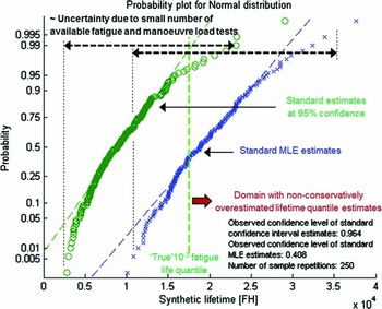
Figure 22 shows 250 repetitions of estimating the same conservative lifetime quantile with the standard method. Seven virtual fatigue tests and 15 virtual tests per manoeuvre were newly performed per repetition. It shows that if no confidence interval would be computed, only about 40% of the lifetime predictions would actually meet the 0.999 reliability requirement. This can be understood by noting that the estimator of the variance, most notably of fatigue strength, is biased towards underestimating the variance. Straightforward simulations confirm that it is ‘normal’ to underestimate the standard deviation in roughly 60% of the cases if only seven tests are done. In case of the standard fatigue life prediction method, this automatically means that the lifetime percentile is non-conservatively overestimated in 60% of the cases, as strength dominates the prediction. However, Fig. 22 shows that if the 10−3 lifetime quantile is computed with a single-sided 95% confidence interval, then 241 out of 250 (96.4%) of repeated predictions met the 0.999 reliability requirement. This demonstrates that the targeted 95% confidence level is met.
Testing of the standard fatigue life prediction method for realistically small samples.

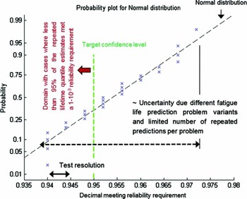
The test as in Fig. 22 was repeated 25 times for redrawn synthetic problems. Each redrawing from Equation (5.2) generates a slightly different fatigue life prediction problem by modifying the overall behaviour of the distributed flight regime loads. This approach explicitly tests the repeatability of the accurate behaviour of the standard method. The distribution of the decimal meeting the reliability requirement is shown in Fig. 23. Following Equation (4.6), approximately ‘one-sigma’ confidence intervals of the realised confidence levels themselves have an approximate width of 2.8%. Therefore, it may be concluded that the standard method yields practically perfect estimates, at least for the tested problem family. To further increase confidence in the accuracy of the standard method, the test, as in Fig. 23, is repeated, but while simulating that ‘only’ seven, instead of 15, manoeuvre load tests were performed per manoeuvre. So the relative uncertainty in estimated manoeuvre loads is increased. The realised confidence levels followed a comparable normal distribution, as in Fig. 23, but with slightly increased variance (imprecision). The observed ‘bottom-of-scatter’ of the decimal meeting the reliability requirement reduced slightly from to 91.2%, instead of 94% before. Repeating the test, but estimating a 10−6 lifetime quantile and simulating only 50 instead of 250 predictions per repetition, demonstrated a ‘bottom-of-scatter’ of the decimal meeting the reliability requirement of 86%.
Repeated testing of the standard fatigue life prediction method for realistically small samples.

Overall, this indicates that the error that the method generally makes by neglecting any effects of uncertainty in loads is, in practice, not too significant in comparison to the effects of uncertainty in strength, which is duly accounted for.
5.3.2 Simulation-based method
The new simulation-based method is first tested by checking if it indeed predicts a 10−3 probability of failure for the lifetime that is already known to be the 10−3 quantile of the ‘true’ reference lifetime distribution. The predicted P fail may not be lower than 10−3 for 95% of the load and strength sampling repetitions when the method targets a 95% single-sided confidence interval. Figure 24 shows that 5/100 of the repeated predictions were too optimistic regarding the probability of failure of the true 10−3 lifetime quantile. This is practically ‘perfect’ performance when considering the precision of this ‘true’ reference. The test, as in Fig. 24, is also repeated, while simulating that ‘only’ seven manoeuvre load tests were performed per manoeuvre. Then, 89/100 MLE estimates and 99/100 upper confidence level estimates were observed to meet the actual reliability requirement. This overly conservative result is believed to be caused by an over-conservatively designed custom procedure that hedges practical issues in fitting multi-dimensional distributions through few sample points. The authors are confident though, that adjustments in the fitting procedure, possibly in combination with more bootstraps per repeated sample, will yield more accurate results.
Testing of the simulation-based fatigue life substantiation model for realistically small samples. The simulation used 150 samples per subset, a strength distribution discretised in 25 intervals and 25 bootstraps per repeated sample. This is a computationally ‘cheap’ configuration.

Finally, the test is repeated again, but now for a more challenging and realistic 10−6 lifetime quantile and while simulating that 15 load samples are available per manoeuvre. The result demonstrated that 7/25 (28%) MLE estimates were conservative and that 23/25 (92%) upper confidence level estimates were conservative, thereby indicating that the simulation-based method can accurately predict 10−6 lifetime quantiles under small sample size conditions and using a ‘cheap’ computational setting, such as in Fig. 24.
The practical engineering problem is, however, not to predict P fail of a given lifetime, but rather to predict a lifetime that meets a reliability requirement (i.e. 0.999). Hence, a Reliability Based Design Optimization (RBDO) application was developed to use the simulation-based lifetime substantiation model to ‘design’ lifetimes that meet a reliability requirement. Figure 25 shows an illustrative result from the RBDO application.
Illustrative result from a custom RBDO application to predict fatigue life using the simulation-based fatigue life substantiation model. Note that P fail estimates around the same lifetime do not differ much, demonstrating the high precision of SS in the newly proposed method (i.e. with 150 samples per subset).

Figure 26 shows 50 repetitions of estimating the same conservative 10−3 lifetime quantile with the custom RBDO application, while having only seven fatigue and 15 manoeuvre load tests available. It shows that none of the repeated lifetime designs fell below the ‘true’ 10−3 lifetime quantile. As a 95% upper single sided confidence level was targeted, this test clearly demonstrates overly conservative results. The validation test of the simulation-based Pfial (SLL) estimates, as in Fig. 24, was passed successfully. Therefore, the authors are confident that manageable adjustments of the RBDO application will yield more accurate results.
Testing of both the simulation-based (red, ‘+’ for MLE and ‘*’ for confidence interval estimates) and standard (blue, ‘o’ for MLE and ‘□’ for confidence interval estimates) fatigue life quantile prediction models. The simulation used 150 samples per subset, a strength distribution discretised in 20 intervals and 25 bootstraps per repeated sample.

5.3.3 Simultaneous comparison
The results in Fig. 26 also allow direct comparison between the simulation-based and analytical method. The test result demonstrates that lifetime quantiles designed by the simulation-based method are similar to estimates from the standard method, though somewhat over-conservative. In general though, it seems that for the tested problem family and with realistically small sample sizes, the ideally attainable precision in estimating a reliable lifetime is simply governed by the precision up to which a quantile of a lognormal strength distribution can be estimated.
6.0 CONCLUSIONS
This work confirms that, under idealised circumstances, a fundamental and non-conservative error is made when the reliability of a predicted fatigue life is substantiated using only the distribution of fatigue strength and simplifying the flight manoeuvre load distributions to their mean values. As a solution, a new simulation-based fatigue life prediction method was successfully validated and was shown to yield accurate results under all described test conditions.
However, it is also demonstrated that the simple analytical method does, nevertheless, feature practically perfect performance under all studied realistic engineering conditions. Direct comparison under these realistic conditions between the analytical and simulation-based method actually revealed no practically significant differences in precision and accuracy. This means that under small sample size conditions, uncertainties in manoeuvre loads may be fully neglected and the full reliability substantiation may be derived from the fatigue strength distribution only.
Future work may include expansion of the synthetic test conditions to estimate boundaries for reliable application of the analytical and simulation-based methods. Expanded test conditions may include:
-
• Increased variation in manoeuvre loads
-
• A broad range of S-N curve shapes, strength variations and mission profiles
Additionally, future work may also include a detailed study on the numerical efficiency of the presented methods.
It is recommended to only make use of the new and complex simulation-based method when circumstances are encountered where the simple and easy-to-apply analytical method is clearly not applicable i.e. when variance and uncertainties from manoeuvre loads are no longer insignificant in comparison to variance and uncertainty from fatigue strength.
Finally, given the work's modelling assumption that only full-scale component fatigue tests can provide relevant data to estimate an S-N-P curve, emphasis is put onto the importance of properly mitigating uncertainty coming from inadvertent inaccurate fatigue strength estimates, due to availability of only few samples. The reach of such uncertainty is clearly exemplified. It is therefore strongly recommended to explicitly determine a confidence interval for any critical fatigue life quantile prediction and clearly state modelling assumptions. This may prevent misconceptions on the reliability that can really be guaranteed by statistical methods.
ACKNOWLEDGEMENTS
Funded with the support of the German Federal Ministry of Economics and Energy.
Editorial suggestions and anonymous peer-review enabled to significantly improve and correct the article.