


1 Introduction
A disk rotating at the bottom of a fixed cylindrical tank partially filled with a liquid induces a flow that potentially shows various instability patterns, such as rotating polygons, switching and sloshing phenomena (see Vatistas Reference Vatistas1990; Jansson et al. Reference Jansson, Haspang, Jensen, Hersen and Bohr2006; Suzuki, Iima & Hayase Reference Suzuki, Iima and Hayase2006; Tasaka & Iima Reference Tasaka and Iima2009; Iima & Tasaka Reference Iima and Tasaka2016; Tasaka & Iima Reference Tasaka and Iima2017). Out of these experimental studies, phase diagrams have been established using two parameters, namely, the initial liquid height and angular speed of the disk (see Jansson et al. Reference Jansson, Haspang, Jensen, Hersen and Bohr2006; Bach et al. Reference Bach, Linnartz, Vested, Andersen and Bohr2014; Iga et al. Reference Iga, Yokota, Watanabe, Ikeda, Niino and Misawa2014). The high Reynolds numbers prevailing in these experiments preclude a realistic numerical simulation of such configurations.
An inviscid model for the axisymmetric base state on which these patterns grow has been proposed by Bergmann et al. (Reference Bergmann, Tophøj, Homan, Hersen, Andersen and Bohr2011) and later on improved by Tophøj et al. (Reference Tophøj, Mougel, Bohr and Fabre2013) and Fabre & Mougel (Reference Fabre and Mougel2014). Despite their simplicity, these models were able to capture the occurrence of patterns in terms of wave resonances (see also Mougel et al. Reference Mougel, Fabre, Lacaze and Bohr2017). In a recent asymptotic analysis of the base flow, Iga (Reference Iga2017) gives an in-depth characterisation of the internal and boundary layers: velocity profiles, scaling laws…This analysis assumes that the flow is laminar, which is a strong assumption. In fact, instabilities can appear at Reynolds number values much smaller than that where the rotating polygons settle in. In most experiments, having a typical length scale of the order of 10 cm and using water as a working fluid, these instabilities break the rotational symmetry of the velocity field long before the surface even starts to deform perceptibly. An azimuthal wave propagates in the same direction as that of the disk (Young, Sheen & Hwu Reference Young, Sheen and Hwu1995; Lopez et al. Reference Lopez, Marques, Hirsa and Miraghaie2004; Poncet & Chauve Reference Poncet and Chauve2007; Kahouadji, Martin Witkowski & Le Quéré Reference Kahouadji, Martin Witkowski and Le Quéré2010). As the disk-rotation speed is increased, turbulence develops on these large scale structures. At sufficiently high disk-rotation speed, the Froude number is no longer small: the free surface is strongly deformed and may form polygons. There is thus a transitional regime that bridges both types of instabilities.
The aim of the present work is to gain knowledge of this transitional regime by studying the mean axisymmetric flow and the fluctuations using direct numerical simulations and experimental measurements. The flow parameters chosen in the present work mostly match those of the experiment of Bergmann et al. (Reference Bergmann, Tophøj, Homan, Hersen, Andersen and Bohr2011) for which velocity measurements are available. The paper is structured as follows: the experimental set-up and the numerical methods are introduced in § 2. In § 3, the steady axisymmetric flow solution is presented, and the effects of Froude and Reynolds numbers are discussed. Section 4 describes how unsteadiness and three-dimensionality affect the axisymmetric mean flow structure. Experimental measurements are carried out to assess the relevance of the numerical simulations. Discussions and comparisons with previous available models are given in § 5.
2 Configuration and methods
The configuration is represented in figure 1(a). The cylindrical tank of inner radius
 $R$
is filled with a layer of liquid with density
 $\unicode[STIX]{x1D70C}_{l}$
and kinematic viscosity
 $\unicode[STIX]{x1D708}$
. At rest, the layer has a uniform height
 $H$
above the bottom disk. When the disk rotates at angular speed
 $\unicode[STIX]{x1D6FA}$
, the surface deforms and may become non-axisymmetric and time-dependent.
(a) Flow configuration. (b) Experimental set-up.

Our experimental set-up (see figure 1
b) is a modified version of the one used in Moisy et al. (Reference Moisy, Doaré, Pasutto, Daube and Rabaud2004). The tank is made of Plexiglas and the heavy brass alloy rotating disk is driven by a DC brushed motor with a tachometer closed-loop speed control. The inner radius of the cylindrical tank is 140 mm and the gap between disk and cylinder is 0.7 mm. Laser-Doppler velocimetry (LDV) is carried out using a Dantec BSA system fastened to a horizontal displacement platform. It consists in a continuous argon-ion laser with wavelength 660 nm and power 25 mW. Hollow silver-coated glass spheres with a diameter of
 $10~\unicode[STIX]{x03BC}\text{m}$
are seeded in the fluid. The temperature is monitored during the experiment and its variation did not exceed
 $2\,^{\circ }\text{C}$
.
In the following, variables
 $R,R\unicode[STIX]{x1D6FA}$
and
 $\unicode[STIX]{x1D70C}_{l}$
are respectively chosen as reference length, velocity and density scales to make all quantities dimensionless. The flow inside the tank is characterised by four dimensionless parameters, namely the aspect ratio
 $G$
, the Reynolds number
 $Re$
, the Froude number
 $Fr$
, indicative of the deformation of the surface, and the Weber number
 $We$
, which quantifies inertia with respect to surface tension:
 $$\begin{eqnarray}G=\frac{H}{R},\quad Re=\frac{R^{2}\unicode[STIX]{x1D6FA}}{\unicode[STIX]{x1D708}},\quad Fr=\frac{R\unicode[STIX]{x1D6FA}^{2}}{g},\quad We=\frac{\unicode[STIX]{x1D70C}_{l}\unicode[STIX]{x1D6FA}^{2}R^{3}}{\unicode[STIX]{x1D70E}},\end{eqnarray}$$
where
 $g$
stands for the gravity acceleration and
 $\unicode[STIX]{x1D70E}$
for the surface tension between gas and liquid. All physical properties of the liquid are assumed constant. In all cases investigated here
 $We$
is found large, which indicates that surface tension effects hardly affect the surface profile and will not be considered in the following.
Besides experiment, two in-house numerical codes are used to study axisymmetric flow states. The first one, ROSE (ROtating Surface Evolution) computes steady states of the liquid phase with surface tension. Using cylindrical coordinates
 $(r,\unicode[STIX]{x1D703},z)$
with the origin at the centre of the bottom disk, the steady Navier–Stokes equations are written as
 $$\begin{eqnarray}\left.\begin{array}{@{}c@{}}\displaystyle 0=r\unicode[STIX]{x1D714}-\left(\frac{\unicode[STIX]{x2202}^{2}\unicode[STIX]{x1D713}}{\unicode[STIX]{x2202}r^{2}}-\frac{1}{r}\frac{\unicode[STIX]{x2202}\unicode[STIX]{x1D713}}{\unicode[STIX]{x2202}r}+\frac{\unicode[STIX]{x2202}^{2}\unicode[STIX]{x1D713}}{\unicode[STIX]{x2202}z^{2}}\right)\\ \displaystyle 0=\frac{\unicode[STIX]{x2202}}{\unicode[STIX]{x2202}r}\left(\frac{1}{r}\frac{\unicode[STIX]{x2202}\unicode[STIX]{x1D713}}{\unicode[STIX]{x2202}z}\unicode[STIX]{x1D714}\right)-\frac{\unicode[STIX]{x2202}}{\unicode[STIX]{x2202}z}\left(\frac{1}{r}\frac{\unicode[STIX]{x2202}\unicode[STIX]{x1D713}}{\unicode[STIX]{x2202}r}\unicode[STIX]{x1D714}\right)-\frac{\unicode[STIX]{x2202}}{\unicode[STIX]{x2202}z}\left(\frac{\unicode[STIX]{x1D6E4}^{2}}{r^{3}}\right)-\frac{1}{Re}\left(\frac{\unicode[STIX]{x2202}^{2}\unicode[STIX]{x1D714}}{\unicode[STIX]{x2202}r^{2}}+\frac{1}{r}\frac{\unicode[STIX]{x2202}\unicode[STIX]{x1D714}}{\unicode[STIX]{x2202}r}-\frac{\unicode[STIX]{x1D714}}{r^{2}}+\frac{\unicode[STIX]{x2202}^{2}\unicode[STIX]{x1D714}}{\unicode[STIX]{x2202}z^{2}}\right)\\ \displaystyle 0=\frac{\unicode[STIX]{x2202}}{\unicode[STIX]{x2202}r}\left(\frac{\unicode[STIX]{x2202}\unicode[STIX]{x1D713}}{\unicode[STIX]{x2202}z}\unicode[STIX]{x1D6E4}\right)-\frac{\unicode[STIX]{x2202}}{\unicode[STIX]{x2202}z}\left(\frac{\unicode[STIX]{x2202}\unicode[STIX]{x1D713}}{\unicode[STIX]{x2202}r}\unicode[STIX]{x1D6E4}\right)-\frac{r}{Re}\left(\frac{\unicode[STIX]{x2202}^{2}\unicode[STIX]{x1D6E4}}{\unicode[STIX]{x2202}r^{2}}-\frac{1}{r}\frac{\unicode[STIX]{x2202}\unicode[STIX]{x1D6E4}}{\unicode[STIX]{x2202}r}+\frac{\unicode[STIX]{x2202}^{2}\unicode[STIX]{x1D6E4}}{\unicode[STIX]{x2202}z^{2}}\right)\end{array}\right\}\end{eqnarray}$$
using Stokes’ streamfunction
 $\unicode[STIX]{x1D713}$
, azimuthal vorticity
 $\unicode[STIX]{x1D714}$
and angular momentum
 $\unicode[STIX]{x1D6E4}$
. These latter quantities are linked to velocity
 $\boldsymbol{V}=(V_{r},V_{\unicode[STIX]{x1D703}},V_{z})$
via
 $$\begin{eqnarray}V_{r}=\frac{1}{r}\frac{\unicode[STIX]{x2202}\unicode[STIX]{x1D713}}{\unicode[STIX]{x2202}z},\quad V_{z}=-\frac{1}{r}\frac{\unicode[STIX]{x2202}\unicode[STIX]{x1D713}}{\unicode[STIX]{x2202}r},\quad \unicode[STIX]{x1D714}=\frac{\unicode[STIX]{x2202}V_{r}}{\unicode[STIX]{x2202}z}-\frac{\unicode[STIX]{x2202}V_{z}}{\unicode[STIX]{x2202}r},\quad \unicode[STIX]{x1D6E4}=rV_{\unicode[STIX]{x1D703}}.\end{eqnarray}$$
Mainly for numerical reasons, surface tension is introduced in the normal stress balance at the air–liquid interface (this was found to solve the convergence problem discussed in Kahouadji & Martin Witkowski (Reference Kahouadji and Martin Witkowski2014)) through
 $\boldsymbol{n}(\unicode[STIX]{x1D64F}_{air}-\unicode[STIX]{x1D64F})\boldsymbol{n}=\unicode[STIX]{x1D70E}\unicode[STIX]{x1D735}\boldsymbol{\cdot }\boldsymbol{n}$
where
 $\unicode[STIX]{x1D64F}$
(respectively
 $\unicode[STIX]{x1D64F}_{air}$
) is the stress tensor on the liquid (respectively air) side,
 $\boldsymbol{n}=(-h^{\prime },0,1)^{t}/(1+h^{\prime 2})$
is the unit outwards normal vector at the surface
 $z=h(r)$
. The deformed meridional domain
 $(r,z)\in [0,1]\times [0,h(r)]$
is adapted to the free surface and mapped to a rectangular one
 $(\unicode[STIX]{x1D709},\unicode[STIX]{x1D702})\in [0,1]\times [0,G]$
, allowing for a Cartesian mesh of
 $N_{r}$
(respectively
 $N_{z}$
) points in the radial (respectively axial) direction in this transformed coordinate setting (Kahouadji & Martin Witkowski Reference Kahouadji and Martin Witkowski2014). The solution is obtained by iterations over the two following steps: (i) system (2.2) is mapped to the rectangular domain, discretised and solved using a Newton–Raphson procedure with a prescribed distribution
 $h(r)$
; (ii) the velocity field obtained at convergence is inserted into the normal stress balance equation which is solved to yield a corrected
 $h(r)$
distribution.
As a second numerical tool, we use the finite-volume DNS (direct numerical simulation) code Sunfluidh that simulates two-dimensional (2-D) and 3-D unsteady incompressible flows. The Navier–Stokes equations are discretised on a staggered grid with second-order accuracy in both time and space and the zero velocity divergence is ensured by an incremental projection method. Further details can be found in Tuerke et al. (Reference Tuerke, Pastur, Fraigneau, Sciamarella, Lusseyran and Artana2017). Sunfluidh also implements a level-set method to tackle interfaces.
3 Steady axisymmetric flow
This section is aimed at describing the structure of the steady axisymmetric solutions (system (2.2)) and investigating the effects of varying Froude and Reynolds numbers. The results are obtained by ROSE using
 $N_{r}\times N_{z}=501\times 101$
,
 $401\times 201$
and
 $401\times 401$
equispaced grid points for aspect ratios
 $G=0.1856$
,
 $0.5$
and
 $1$
respectively.
In order to evaluate how spatial resolution affects numerical solutions, we consider the configuration
 $G=0.1856$
,
 $Re=10\,000$
and first check flat surface computations, by setting
 $Fr=0$
in ROSE and using the monophasic version of Sunfluidh. ROSE calculations were conducted on four different grids
 $N_{r}\times N_{z}=251\times 51$
,
 $501\times 101$
,
 $1001\times 201$
and
 $2001\times 401$
with equispaced grid points. Maximum and minimum values of the streamfunction, radial and axial velocity components were shown to vary less than 1.95 %, 0.44 % and 0.09 % respectively from the first three grid systems to the finest one, so that the grids selected in the present paper for ROSE computations ensure sufficient precision. Sunfluidh calculations were conducted on the three uniform grids
 $N_{r}\times N_{z}=128\times 32$
,
 $256\times 64$
and
 $512\times 128$
. The maximum and minimum velocity components were found to differ by less than 2.6 %, 0.95 % and 0.16 % respectively from those of the most resolved ROSE computation.
Validations on configurations with a deformed surface at
 $Fr=1$
were also performed. For ROSE, the solution is sought in a monophasic deformed domain (see § 2) on grid
 $Nr\times Nz=501\times 101$
while for Sunfluidh, the steady two-phase flow solution is determined in the domain
 $(r,~z)\in [0,~1]\times [0,~0.5]$
on a regular mesh
 $Nr\times Nz=256\times 128$
from an initially rest state with a liquid–air interface at
 $z=G$
. The extrema of
 $V_{r}$
and
 $V_{z}$
were found to differ only by approximately
 $1\,\%$
between the two codes, which is fully satisfactory as these two techniques to deal with surface deformation are completely different.
3.1 Effect of Froude number
Effect of the Froude number on the steady axisymmetric flow structure for
 $G=0.1856$
,
 $Re=10\,000$
,
 $We=1263.6$
and, from top to bottom,
 $Fr=0.01$
,
 $0.2464$
,
 $1$
. (a,c,e) Streamlines of the meridional circulation consisting of 21 equispaced solid contours of
 $\unicode[STIX]{x1D713}$
between 0 and
 $\unicode[STIX]{x1D713}_{max}=(0.0034,0.0035,0.0035)$
and one dashed contour at value
 $(1/2)\unicode[STIX]{x1D713}_{min}$
with
 $\unicode[STIX]{x1D713}_{min}=(-1.993,-1.975,-1.825)\times 10^{-4}$
. (b,d,f) Isocontours of the azimuthal velocity
 $V_{\unicode[STIX]{x1D703}}$
, with 21 equispaced contours between 0 and 1. The thick black lines denote the free surface.

Deviation
 $(h(r)-G)/Fr$
of the free surface rescaled by
 $Fr$
. Same parameters as figure 2.

Effect of the Froude number on the velocity of the steady axisymmetric flow for
 $G=0.1856$
,
 $Re=10\,000$
and
 $We=1263.6$
, for
 $Fr=0.01$
(red solid),
 $Fr=0.2464$
(blue dash) and
 $Fr=1$
(brown dash-dot). Radial distributions of (a)
 $V_{\unicode[STIX]{x1D703}}$
and (b)
 $V_{r}$
at the free surface; radial distributions of (c)
 $V_{\unicode[STIX]{x1D703}}$
and (d)
 $V_{r}$
at half the interface height
 $z=h(r)/2$
; axial distribution at
 $r=0.8$
of (e)
 $V_{\unicode[STIX]{x1D703}}$
and (f)
 $rV_{r}$
, plotted as functions of
 $z/h(0.8)$
.

Figure 2 shows the flow structure obtained at large Reynolds number (
 $Re=10\,000$
), consisting of a central region with pure solid body rotation at the exact velocity of the disk (b,d,f) and an outer region with a meridional circulation (a,c,e). This circulation is relatively weak, as indicated by the low levels of
 $\unicode[STIX]{x1D713}\leqslant 0.0035$
. A striking feature is that the overall flow arrangement is hardly modified when the Froude number is varied from
 $Fr=0.01$
(figure 2
a,b) where surface deformation is negligible, to
 $Fr=1$
(figure 2
e,f) where the surface is strongly deformed and almost touches the bottom disk at the centre. For the Newton bucket (i.e. solid body rotation), the deviation
 $h(r)-G$
is proportional to the Froude number. Using numerical simulations with an undeformed free surface, Piva & Meiburg (Reference Piva and Meiburg2005) proposed a first-order approximation for the surface elevation
 $h(r)$
based on the normal stress balance, yielding a scaling proportional to
 $Fr$
. Kahouadji & Martin Witkowski (Reference Kahouadji and Martin Witkowski2014) observed and interpreted such a scaling for weaker deformations and moderate Reynolds numbers. Figure 3 shows the rescaled surface deformation
 $(h(r)-G)/Fr$
for the set of parameters of figure 2: this scaling remains here a fair approximation, even though at
 $Fr=1$
the surface deformation is of the same order of magnitude as that of the fluid-layer thickness. The main effect of free surface deformation is thus to constrain the flow field: this is quantitatively shown in figure 4 where some velocity components at the surface, at half-depth or at fixed radius are extracted for different Froude numbers and almost superpose when
 $z$
is rescaled by the local depth
 $h(r)$
. This feature is found to be robust for Reynolds numbers greater than
 $Re=1000$
.
3.2 Effect of Reynolds number
As the Froude number influences the flow structure only marginally, flat surface cases (
 $h=G$
) are conveniently chosen to study the effects of
 $Re$
at lower numerical cost. Figure 5 illustrates how the flow evolves as
 $Re$
is increased from low values.
One first observes the gradual formation of boundary layers at the rotating disk and at the side wall, but also at the free surface (hereafter called the top layer) and at the edge of the solid-rotation core (core layer). These layers then become thinner as Reynolds is increased. The selected grids ensure at least 15 grid points in each layer viewed in the meridional plane even at the highest Reynolds number
 $Re=19~500$
. An overshoot of the azimuthal velocity arises at mid-radius in the top layer, similar to the one observed by Iwatsu (Reference Iwatsu2004): the fluid locally spins faster than the disk at the same radius (see the contour of azimuthal velocity in figure 5 at
 $Re\geqslant 10\,000$
) as a consequence of the inward flow convecting angular momentum with weak dissipation. This overshoot at this location is captured for all of the above grid resolutions.
Effect of the Reynolds number on the steady axisymmetric flow structure for
 $G=0.1856$
,
 $Fr=0$
and, from top to bottom,
 $Re=300$
,
 $1200$
,
 $10\,000$
,
 $19\,500$
. Same representation as in figure 2 with here
 $\unicode[STIX]{x1D713}_{max}=(0.0035,0.0074,0.0034,0.0024)$
and
 $\unicode[STIX]{x1D713}_{min}=(0,0,-1.993,-1.447)\times 10^{-4}$
.

Maximum of (a)
 $\unicode[STIX]{x1D713}$
,
 $V_{z}$
and (b)
 $rV_{r}$
as functions of
 $Re$
, for
 $Fr=0$
and two values of aspect ratio
 $G=0.1856$
(black/lower curves) and
 $0.5$
(blue/upper curves).

The existence of two regimes prevailing at low and large
 $Re$
is best illustrated in figure 6. The maximum
 $\unicode[STIX]{x1D713}_{max}$
of Stokes’ streamfunction quantifies the strength of the meridional recirculation: at
 $G=0.1856$
, this quantity (figure 6
a) is first found proportional to
 $Re$
, and so do the maxima
 $(rV_{r},V_{z})_{max}$
of
 $rV_{r},V_{z}$
(figure 6
b). Indeed, in the viscous regime up to
 $Re=300$
, length scales are of order 1 as well as the azimuthal velocity; balancing the two last terms of the vorticity equation in system (2.2) leads to a scaling proportional to
 $Re$
for the meridional flow.
For
 $Re\approx 1500$
, this trend has stopped:
 $(rV_{r},V_{z})_{max}$
saturate at a constant value close to
 $0.1$
. When the Reynolds number is further increased, the above structure no longer holds: an Ekman-like layer with typical thickness
 $\unicode[STIX]{x1D6FF}\propto Re^{-1/2}$
forms on the rotating disk at the same time as other layers, as will be described in § 3.3. In the Ekman layer,
 $V_{r}$
scales as
 $r$
(von Kármán Reference von Kármán1921) and thus
 $(rV_{r})_{max}$
is of order 1, independent of
 $Re$
– same for
 $(V_{z})_{max}$
in the side layer by flow conservation arguments. As
 $\unicode[STIX]{x1D6FF}\propto Re^{-1/2}$
, the meridional recirculation strength
 $\unicode[STIX]{x1D713}_{max}\propto \unicode[STIX]{x1D6FF}\times (rV_{r})_{max}$
is thus expected to decrease as
 $Re^{-1/2}$
as well, due to the thinning of the layers inside which most of the circulation takes place. This is observed in figure 6(a): for
 $G=0.1856$
, the interpolation gives an exponent of
 $-0.49$
. This scaling is fully consistent with the in-depth asymptotic analysis of the bottom and side wall layers performed by Iga (Reference Iga2017). Figure 6 also shows the results for another aspect ratio,
 $G=0.5$
: the same scalings are observed. Quantities
 $(rV_{r},V_{z})_{max}$
saturate around the same value 0.1, which is not surprising as the scalings for the Ekman boundary layer do not involve
 $G$
. However the recirculation in the low-
 $Re$
regime is far more intense at
 $G=0.5$
, which is due to a larger recirculation zone. This mechanically leads to a shift of the critical Reynolds number for the change of regime towards smaller values, around 400 for
 $G=0.5$
.
3.3 Flow structure at large Reynolds number
Structure of the steady axisymmetric flow at
 $Re=10\,000$
for
 $G=0.5$
(a,b) and
 $G=1$
(c,d). (a,c) Streamlines of the meridional circulation with 25 equispaced contours between
 $\unicode[STIX]{x1D713}_{min}=(-1.8181,-2.87)\times 10^{-4}$
(dashed line for negative streamfunction) and
 $\unicode[STIX]{x1D713}_{max}=(0.0038,0.0043)$
, respectively for
 $G=(0.5,1.0)$
. (b,d) Isocontours of
 $V_{\unicode[STIX]{x1D703}}$
, with 25 equispaced contours between 0 and 1.

Figure 7 gives a more general picture of the steady flow obtained in the axisymmetric framework at large Reynolds number
 $Re=10\,000$
(i.e. above the critical Reynolds number introduced previously), obtained for aspect ratio
 $G=0.5$
and
 $G=1.0$
. The main features already observed at
 $G=0.1856$
are also present here: a solid body rotation (hereafter denoted as SBR) in the central part and a meridional recirculation (hereafter denoted as MR) at the periphery, with four layers. However the core layer has an intricate sinuous shape and feeds a lower region stretching down to the disk. Further increasing the aspect ratio to
 $G=1$
(see figure 7
c) shows that the size of the upper sub-cell changes only slightly: its axial extent increases from 0.2 to 0.25. Most of the increase in fluid depth is passed to the extension of the lower mostly
 $z$
-independent region, while the bottom layer with an Ekman-like structure is hardly modified (Iga Reference Iga2017). For
 $G=0.1856$
, this lower region is only slightly visible at the highest Reynolds number (see figure 5).
The key point to close existing theoretical models (see discussion in § 5) is to determine the radius
 $r_{s}$
of the boundary between SBR and MR regions (Tophøj et al.
Reference Tophøj, Mougel, Bohr and Fabre2013; Fabre & Mougel Reference Fabre and Mougel2014; Iga Reference Iga2017). This parameter can be tentatively determined from simulation results. To do so, we define
 $r_{s}$
as the location of the first maximum of
 $V_{\unicode[STIX]{x1D703}}(r,z=G/4)$
, as depicted in figure 4(c): we chose
 $z=G/4$
in order to get rid of the influence of the upper cell and the bottom layer. Figure 8 shows the decrease of
 $r_{s}$
as
 $G$
is increased, which confirms previous studies (Tophøj et al.
Reference Tophøj, Mougel, Bohr and Fabre2013; Iga Reference Iga2017). This trend is a consequence of the balance between side wall dissipation and energy injection at the rotating disk below the MR region.
Location
 $r_{s}$
of the boundary between SBR and MR regions determined at
 $z=G/4$
as a function of Reynolds number
 $Re$
for 4 different aspect ratios
 $G$
, deduced from ROSE computations.

The axial velocity component
 $V_{z}$
at
 $r=r_{s}$
has been plotted as a function of
 $G-z$
in figure 9. Coordinate
 $G-z$
has been used so that the free surfaces at
 $G-z=0$
coincide for the three aspect ratios. It is observed that the size of the upper cell indeed weakly varies with
 $G$
, as stated above. Moreover, the graph reveals a flow reversal (
 $V_{z}<0$
) similar to that observed in vortex-breakdown bubbles for rotating-lid experiments (Escudier Reference Escudier1984). This analogy has already been pointed out by Iwatsu (Reference Iwatsu2004), Piva & Meiburg (Reference Piva and Meiburg2005) and Herrada, Shtern & Lopez-Herrera (Reference Herrada, Shtern and Lopez-Herrera2013) and is sometimes referred to as ‘off-axis vortex breakdown’.
Axial velocity component
 $V_{z}(r_{s},G-z)$
at
 $Re=10\,000$
for
 $G=0.1856$
,
 $0.5$
and
 $1$
.

The axisymmetric flow solutions obtained here are physically relevant up to a critical value of the Reynolds number for which the flow becomes unsteady. Using Newton’s method implemented in ROSE allows us to go beyond this critical value by the continuation technique. However, exploring further these steady axisymmetric unstable branches of solutions at higher Reynolds number values is eventually limited by a non-trivial dynamical behaviour. This is the reason why the curves in figure 8 could not be pursued beyond
 $Re=19\,000$
–
 $23\,000$
. An alternative way is then to use unsteady computations of the three-dimensional flow.
4 Three-dimensional flow
For a given aspect ratio, there is a large range of Reynolds numbers for which the velocity field is yet three-dimensional and unsteady while the free surface deforms but remains almost axisymmetric. We focus here on this transitional regime that extends up to the occurrence of rotating polygons. The critical Reynolds number value that determines the lower bound of the transitional regime and the associated critical azimuthal wavenumber strongly depends on the fluid aspect ratio. These critical parameters were determined for
 $G$
varying from
 $0.036$
to
 $0.107$
experimentally by Poncet & Chauve (Reference Poncet and Chauve2007) and numerically by Kahouadji et al. (Reference Kahouadji, Martin Witkowski and Le Quéré2010) using linear stability analysis. For
 $G=0.25$
and
 $G=2$
, Lopez et al. (Reference Lopez, Marques, Hirsa and Miraghaie2004) performed a study using nonlinear numerical simulations and experiments. Cogan, Ryan & Sheard (Reference Cogan, Ryan and Sheard2011) extended the computations to the range
 $G=1.5$
to
 $G=3.5$
and Serre & Bontoux (Reference Serre and Bontoux2007) studied
 $G=4$
. All the numerical simulations have assumed a flat horizontal interface.
In this section, we focus on the specific value
 $G=0.1856$
. Assuming a monotonic variation with aspect ratio, we can expect a critical Reynolds number between
 $Re\sim 1450$
given by Lopez et al. (Reference Lopez, Marques, Hirsa and Miraghaie2004) for
 $G=0.25$
and
 $Re\sim 10\,000$
given by Poncet & Chauve (Reference Poncet and Chauve2007) for
 $G=0.107$
. Therefore, we choose the values
 $Re=30\,000$
and
 $81\,400$
in the following as they lie far beyond the threshold and are typical of the transitional regime. Furthermore, the value
 $Re=30\,000$
allows for comparisons between fully resolved simulations and experiments in which the velocities are large enough for accurate LDV measurements.
At such Reynolds number values, the flow is turbulent with coherent structures (see movies 1–3 in the supplementary material, available at https://doi.org/10.1017/jfm.2018.929). The present section characterises the axisymmetric mean flow and fluctuations in the transitional regime, and gives a description of the unsteadiness (§ 4.3).
4.1 Simulations: mean flow and fluctuations
A 3-D simulation is performed at
 $Re=30\,000$
using Sunfluidh. The chosen numerical domain
 $(r,\unicode[STIX]{x1D703},z)\in [0.4,1]\times [0,(2/3)\unicode[STIX]{x03C0}]\times [0,0.1856]$
covers only a part of the physical one: a solid body rotation is assumed for
 $r<0.4$
which is not simulated, and only a third of the full azimuthal extent is considered using periodic boundary conditions along
 $\unicode[STIX]{x1D703}$
, a choice motivated by the prevalence of the
 $m=3$
mode in our experiment (see § 4.2). The 3-D mesh consists of
 $192\times 448\times 128$
cells and is refined along the side wall, above the disk and below the free surface. The radial grid spacing decreases from
 $\unicode[STIX]{x1D6FF}r=4.17\times 10^{-3}$
for
 $r\in [0.4,~0.8]$
continuously to
 $\unicode[STIX]{x1D6FF}r=1.4\times 10^{-3}$
at
 $r=1$
. Along the axial direction, the grid spacing varies from
 $\unicode[STIX]{x1D6FF}z=3.1\times 10^{-3}$
in the bulk to
 $\unicode[STIX]{x1D6FF}z=2\times 10^{-4}$
at the disk and at the surface. The grid spacing in the azimuthal direction is uniform. We impose a Courant–Friedrichs–Lewy (CFL) constraint of 0.2, so that the time step is
 $\unicode[STIX]{x1D6FF}t\approx 7.7\times 10^{-4}$
.
Sunfluidh also allows for unsteady 2-D simulations. A first simulation is undertaken in two dimensions in the domain
 $(r,z)\in [0.4,1]\times [0,0.1856]$
at
 $Re=30\,000$
using the same grid spacing as above along
 $r$
and
 $z$
. Even in the 2-D framework, the flow is found to be unsteady, but it evolves to a statistically permanent regime with mean velocity
 $\overline{\boldsymbol{V}}_{\!2D}$
, defined by averaging
 $\boldsymbol{V}$
over a large time interval
 $\unicode[STIX]{x0394}t=200$
.
In order to save some computation time, the 3-D simulation is started from an instantaneous 2-D field in the permanent regime. After a time period
 $T_{e}$
, the 3-D flow reaches another statistically permanent regime. A mean velocity
 $\overline{\boldsymbol{V}}_{\!3D}$
is defined by averaging over the same time interval
 $\unicode[STIX]{x0394}t$
and over the entire azimuth of the computational domain
 $\unicode[STIX]{x0394}\unicode[STIX]{x1D703}=(2/3)\unicode[STIX]{x03C0}$
:
 $$\begin{eqnarray}\overline{\boldsymbol{V}}_{\!3D}(r,z)=\frac{1}{\unicode[STIX]{x0394}t\unicode[STIX]{x0394}\unicode[STIX]{x1D703}}\int _{0}^{\unicode[STIX]{x0394}\unicode[STIX]{x1D703}}\int _{T_{e}}^{T_{e}+\unicode[STIX]{x0394}t}\boldsymbol{V}(r,\unicode[STIX]{x1D703},z,t)\,\text{d}t\,\text{d}\unicode[STIX]{x1D703}.\end{eqnarray}$$
Streamlines of the meridional circulation for
 $G=0.1856$
,
 $Re=30\,000$
, computed from (a)
 $\overline{\boldsymbol{V}}_{\!2D}$
(respectively (b)
 $\overline{\boldsymbol{V}}_{\!3D}$
). The graph consists of 21 equispaced solid contours of
 $\unicode[STIX]{x1D713}$
between 0 and
 $\unicode[STIX]{x1D713}_{max}=2.1\times 10^{-3}$
(respectively
 $1.98\times 10^{-3}$
) and one dashed contour at value
 $(1/2)\unicode[STIX]{x1D713}_{min}$
with
 $\unicode[STIX]{x1D713}_{min}=-1.12\times 10^{-4}$
(respectively
 $-0.924\times 10^{-4}$
). The locations of the points with maximum and minimum
 $\unicode[STIX]{x1D713}$
are respectively indicated by the red and the blue cross.

Due to Reynolds stresses, the mean flow may differ significantly from that arising from system (2.2). Figure 10 shows the meridional circulations obtained when considering either
 $\overline{\boldsymbol{V}}_{\!2D}$
or
 $\overline{\boldsymbol{V}}_{\!3D}$
at
 $Re=30\,000$
. Some subtle changes are observed in the sub-cell shapes. Concerning the value of
 $\unicode[STIX]{x1D713}_{max}$
however, an extrapolation of the axisymmetric steady solution (curve in figure 6) would lead to prediction of a value
 $1.93\times 10^{-3}$
at
 $Re=30\,000$
, in good agreement with the values obtained by 2-D or 3-D DNS both close to
 $2\times 10^{-3}$
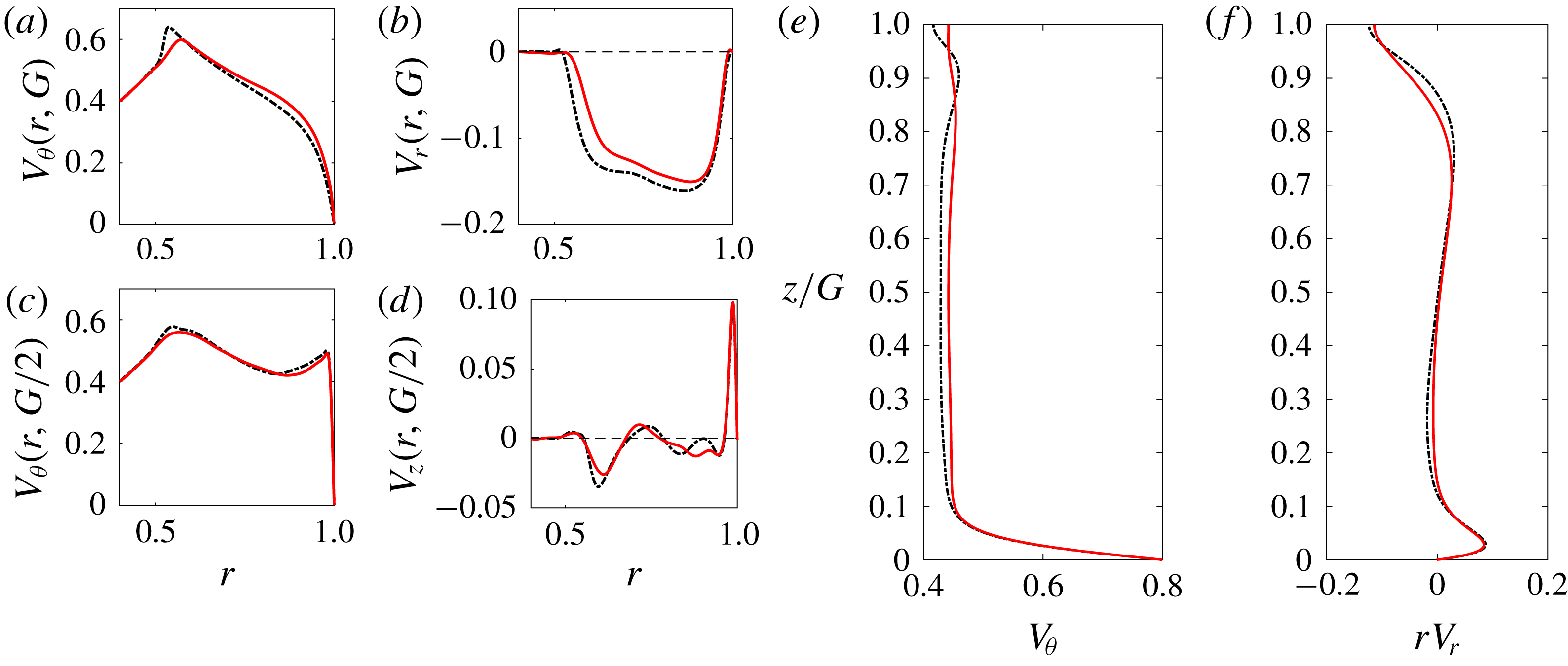
. The mean meridional circulation is thus weakly affected by 3-D effects, as also shown by the velocity profiles in figure 11(b,d,f). Concerning the mean azimuthal velocity component (figure 11
a,c,e), the most striking modification brought by three-dimensionality is the smoothing of the overshoot at the surface in the vicinity of
 $r=0.6$
(figure 11
a).
Profiles of mean velocities
 $\overline{\boldsymbol{V}}_{\!2D}$
(black dash-dotted lines) and
 $\overline{\boldsymbol{V}}_{\!3D}$
(red continuous lines) obtained by DNS for
 $G=0.1856,Re=30\,000$
. Velocity profiles as in figure 4.
4.2 Experiments: mean flow and fluctuations
Velocity measurements have been conducted with a water layer of initial height
 $H=26$
mm so that
 $G\approx 0.1856$
as in Bergmann et al. (Reference Bergmann, Tophøj, Homan, Hersen, Andersen and Bohr2011) (see their figure 12). Two angular speeds of the bottom disk have been chosen in order to match either the Reynolds number used in the numerical simulation of the previous section or the Froude number of Bergmann’s experiment. In the meridional plane, mean and root-mean-square (r.m.s.) values of the azimuthal and axial velocity components were measured along one or several lines of constant
 $z$
.
The first case investigated has an angular speed
 $\unicode[STIX]{x1D6FA}=1.53~\text{rad}~\text{s}^{-1}$
, leading to
 $Re=30\,000$
and
 $Fr=0.0335$
with no noticeable surface deformation. Figure 12 displays the mean and r.m.s. azimuthal velocity component just below the surface as well as the azimuthal and axial components at several heights. The corresponding quantities obtained via the 3-D DNS have also been plotted. Concerning the azimuthal component, the agreement is good except in specific regions: near the side boundary at mid-height (figure 12
b), and near the maximum at the surface, where experimental results do not show any overshoot (figure 12
a). As for the axial velocity component at mid-height (figure 12
c), negative values are found experimentally around
 $r=0.83$
and numerically around
 $r=0.6$
, indicating that the shape of the meridional circulation significantly differs from the experiment to the numerics. We also measured the mean axial velocity profile at other heights (see figure 12
d). The range for which axial velocity measurements can be performed is limited as both incident beams in the tank must remain within the fluid-layer axial extension. For
 $0.38\leqslant z/G\leqslant 0.69$
, the profile was found to be independent of
 $z$
as were the r.m.s. values (not shown). The mismatch between numerics and experiments remains unexplained at this stage. A possible reason could be the fact that surface pollution, especially when water is used as a working fluid, may affect the flow dynamics; its mathematical modelling is still an open issue (Peaudecerf et al.
Reference Peaudecerf, Landel, Goldstein and Luzzatto-Fegiz2017; Moisy, Bouvard & Herreman Reference Moisy, Bouvard and Herreman2018). However, the orders of magnitude for both maximum mean values are in agreement, which is satisfactory since experimental measurements of such a small velocity component are extremely delicate and numerical simulations are demanding.
For the second case shown here, the rotation speed is higher,
 $\unicode[STIX]{x1D6FA}=4.15~\text{rad}~\text{s}^{-1}$
, which corresponds to
 $Re=81~400$
and the same Froude number
 $Fr=0.2464$
as in Bergmann et al. (Reference Bergmann, Tophøj, Homan, Hersen, Andersen and Bohr2011) (their figure 12). Results are displayed in figure 13. At such a high Reynolds number, azimuthal velocity profiles are found independent of
 $z$
in the range
 $0.192\leqslant z/G\leqslant 0.75$
investigated (the upper limitation is due to the strong surface deformation). Moreover, the axial velocity profile at mid-height seems to be robust as it is found to be very close to the one measured at
 $Re=30\,000$
.
Experimental and numerical mean and r.m.s. velocity distributions for the case
 $G=0.1856$
,
 $Re=30\,000$
and
 $Fr=0.0335$
(
 $0$
for numerical simulations). Mean values obtained by LDV (blue circles) and 3-D DNS (black solid line) of (a)
 $V_{\unicode[STIX]{x1D703}}$
at
 $z/G=0.96$
, (b)
 $V_{\unicode[STIX]{x1D703}}$
at
 $z/G=0.5$
and (c)
 $V_{z}$
at
 $z/G=0.5$
. In each case the r.m.s. amplitude is indicated by two curves above and below the mean value (thin dashed and dot-dashed lines). Thick dashed line: disk azimuthal velocity. (d) Measurements of
 $V_{z}$
as function of
 $r$
at different heights.

Experiments at
 $G=0.1856$
,
 $Re=81\,400$
and
 $Fr=0.2464$
. Mean distribution of (a)
 $V_{\unicode[STIX]{x1D703}}$
at different heights and (b)
 $V_{z}$
at
 $z/G=0.5$
(blue circles) with indication of the r.m.s. level.

4.3 Analysis of the unsteady flow
(a) Experiment at
 $G=0.1856$
,
 $Re=30\,000$
and
 $Fr=0.0335$
: top view of the water layer seeded with Kalliroscope flakes. The red circle at
 $r=0.8$
indicates the position of the line captured for the spatio-temporal diagram of figure 15(a). (b) Numerical simulation at
 $G=0.1856$
,
 $Re=30\,000$
and
 $Fr=0$
: snapshot of the axial velocity at
 $z=0.84G$
. The periodic numerical domain
 $(r,\unicode[STIX]{x1D703})\in [0.4,1]\times [0,(2/3)\unicode[STIX]{x03C0}]$
has been replicated along the azimuth; for
 $r<0.4$
(inside the black circle) a zero axial velocity has been plotted.

Sections 4.1 and 4.2 describe the mean axisymmetric flow in the transitional regime and quantify the fluctuation amplitude via r.m.s. values. Hereafter we briefly describe the structure and the frequency spectrum of these fluctuations for the case
 $G=0.1856$
,
 $Re=30~000$
, for which both experiments and simulations are available.
(a) Spatio-temporal diagram of (coloured) grey levels extracted from the experiment displayed in figure 14 along the circle
 $r=0.8$
and (b) corresponding spectrum in the mode–frequency domain.

Even though the free surface remains almost flat in this configuration, a flow structure is evidenced when Kalliroscope flakes are added to the water. Figure 14 reveals a mode with azimuthal wavenumber
 $m=3$
, with a large amplitude at the periphery of the solid body rotation zone. This robust structure rotates in the same direction as the disk, however at a lower angular speed (see movie 1 in supplementary material). A quantitative characterisation is performed by extracting the grey levels from successive video images along the circle of radius
 $r=0.8$
. A spatio-temporal picture is obtained and plotted in figure 15(a). The diagram contains inclined stripes from which we can deduce an angular phase velocity of
 $\unicode[STIX]{x1D71B}=1/0.98~\text{rad}~\text{s}^{-1}=1.02~\text{rad}~\text{s}^{-1}$
. This corresponds to a pattern rotating at an angular velocity close to
 $2/3$
of that of the disk
 $\unicode[STIX]{x1D6FA}=1.53~\text{rad}~\text{s}^{-1}$
, or equivalently to a frequency
 $f=m\unicode[STIX]{x1D71B}/(2\unicode[STIX]{x03C0})$
close to twice the disk frequency
 $f_{d}=\unicode[STIX]{x1D6FA}/(2\unicode[STIX]{x03C0})$
. This is best seen in the spectral domain when applying a 2-D Fourier transform to the spatio-temporal signal: in figure 15(b), the maximum of the spectrum is located at
 $m=3$
and
 $f/f_{d}=1.98$
. Note that a peak at
 $(m,f/f_{d})=(1,1)$
is also visible, presumably associated with the disk rotation.
Numerical simulations bring some useful information on the minimum ingredient to capture this instability. Figure 16(a) shows the evolution of the azimuthal velocity at some probe location for the chained 2-D and 3-D simulations with Sunfluidh. As mentioned earlier, the temporal mean is barely shifted in going from two to three dimensions. However, the r.m.s. value is strongly enhanced in the 3-D simulation. The spectrum associated with the 3-D established state shows a peak at
 $f/f_{d}=2.07$
in full agreement with the above experimental determination.
Comparison at
 $G=0.1856$
,
 $Re=30\,000$
and
 $Fr=0.0335$
(
 $Fr=0$
for the simulation). (a) Simulated evolution of
 $V_{\unicode[STIX]{x1D703}}$
at the probe location
 $(r,~z)=(0.8,0.0928)$
in chained 2-D (dashed) and 3-D (solid) runs; (c) power spectral density (PSD) in the established regime for
 $t>2140$
. (b) Measured azimuthal velocity in the established regime at the same probe location, determined by LDV; (d) corresponding spectrum.

The above findings on the frequency spectrum were eventually corroborated by experimentally measuring the azimuthal velocity using an LDV probe located at the very same location. Signal and spectrum are displayed in figure 16(b,d). A marked frequency peak is found at the same frequency – this peak was also found at all other locations investigated for both axial and azimuthal velocity components. The fluctuation amplitude differs between experiments and numerics depending on the probe location. For the case of figure 16, the discrepancy is relatively strong, but, as illustrated in figure 12(a,b), better agreement can be found at other locations. On the whole, the 3-D simulation restricted to the sector
 $r\in [0.4,1]$
and
 $\unicode[STIX]{x1D703}\in [0,(2/3)\unicode[STIX]{x03C0}]$
is able to catch most of the instability features of the flow in the transitional regime.
This azimuthal modal structure at such relatively large Reynolds number is likely to be related to the primary instability at threshold. Indeed, the angular speed of the observed pattern normalised by that of the disk is close to 2/3, a ratio that we found to be robust with respect to changes in
 $Re$
; at threshold, this same ratio (within approximately 10 %) has been reported from linear stability analyses, whatever the critical azimuthal wavenumber Kahouadji (Reference Kahouadji2011).
5 Discussion and concluding remarks
Which base flow should be used for linear stability analysis is a major question as it is usually a necessary requisite for accurate predictions of bifurcation thresholds. This study gives a better understanding of the base flow structure. Increasing the rotation speed leads, for Reynolds numbers exceeding a value of typically several hundreds, to a regime where most of the meridional circulation takes place within boundary layers. Increasing the rotation speed also enhances surface deformation, with a deviation
 $h(r)-G$
almost proportional to the Froude number. Numerical simulations reveal that this deformation however preserves the overall flow structure. Unsteady 3-D DNS results show little and localised influence on the mean fields. Along with r.m.s. data, these characterisations provide a clear picture of the flow at high Reynolds numbers, far beyond the primary instability threshold.
A comparison between the numerical simulations and existing models is of interest. Iga (Reference Iga2017) suggested that the rotating polygons grow on a laminar base flow at least in the bottom and side wall boundary layers, while the model presented by Tophøj et al. (Reference Tophøj, Mougel, Bohr and Fabre2013) assumes fully developed turbulence. This may deeply impact the angular momentum exchanges between the flow and the walls. As a matter of fact, to close the models, the balance between the angular momentum fed by the bottom disk and dissipated by the side wall is used to find the position of the solid body rotation radius
 $r_{s}$
. In our experiment and simulation, the flow is clearly turbulent.
Nevertheless, in the transitional regime, the bottom and side wall layers studied by Iga (Reference Iga2017) are confirmed and do not differ significantly from those obtained by the mean flow as the r.m.s. is quite small in those layers. In particular the side wall layer could be both accurately measured and simulated with an excellent agreement (figure 12
a,b). Overall, our study shows that the boundary layers are mildly modified by turbulence and most of its structure is captured in the laminar regime. In addition to the boundary layers described by Iga (Reference Iga2017), simulations reveal a top layer along the free surface, an overshoot of the azimuthal velocity at the intersection of the top and the core layers and a sinuous deformation of the core layer. These features of the steady two-dimensional solutions are also present in the mean unsteady 2-D and 3-D flow simulations. The 3-D unsteadiness is found to weaken the sharp overshoot present in two dimensions (figure 11
a) without smoothing it out completely. The presence of the top layer in the simulations implies that the azimuthal and radial velocity profiles at the surface are not representative of the profiles in the bulk. This could be of importance as most simplified models assume a
 $z$
-independent azimuthal velocity profile obtained through surface measurements.
Comparison between azimuthal velocity profiles along the radius for aspect ratios (a)
 $G=0.1856$
, (b)
 $G=0.5$
and (c)
 $G=1$
. Magenta solid: ROSE calculation at
 $Re=10\,000$
and
 $z=G/4$
. Red dotted: distribution from Iga’s (Reference Iga2017) model (the thin black dashed line shows the position of
 $r_{s}^{I}$
as determined in this model respectively at
 $0.57,0.43$
and
 $0.34$
). Black dashed: ideal Rankine vortex model with core size
 $r_{s}^{I}$
. Blue dash-dot: the TMBF model in Mougel (Reference Mougel2014) with correction of the dissipation, leading to values
 $r_{s}^{TMBF}=0.57,0.49$
and
 $0.43$
. Without corrections, this latter model would predict values
 $0.65,0.58$
and
 $0.52$
respectively for the three aspect ratios.

We now compare our computations with two existing models namely those presented by Fabre & Mougel (Reference Fabre and Mougel2014) (hereafter the Tophøj–Mougel–Bohr–Fabre (TMBF) model) and Iga (Reference Iga2017) for three aspect ratios. In these existing models, as stated above,
 $r_{s}$
is a key parameter. Once
 $r_{s}$
is known, the azimuthal velocity field can be derived. An additional matching between the solid body rotation region and the peripheral region, assumed potential, was derived by Iga (Reference Iga2017) in order to remove the unphysical slope discontinuity at
 $r_{s}$
. (It is worth noting that there is a typo in formula (3.64) of Iga (Reference Iga2017) where the term
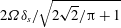 $2\unicode[STIX]{x1D6FA}\unicode[STIX]{x1D6FF}_{s}/\;\sqrt[]{2\;\sqrt[]{2}/\unicode[STIX]{x03C0}+1}$
should be
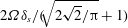 $2\unicode[STIX]{x1D6FA}\unicode[STIX]{x1D6FF}_{s}/(\sqrt[]{2\;\sqrt[]{2}/\unicode[STIX]{x03C0}}+1)$
.) Azimuthal velocity profiles are compared in figure 17. For
 $G=0.1856$
, there is a fair match between the 2-D steady simulation and both theories. The radius
 $r_{s}$
is predicted within a few per cent when compared to the value
 $r_{s}=0.58$
given in figure 12 of Bergmann et al. (Reference Bergmann, Tophøj, Homan, Hersen, Andersen and Bohr2011) and our experiment where
 $r_{s}$
is slightly below
 $0.6$
. As the aspect ratio increases, the results issued from theory deviate significantly from the numerical results: Iga’s model underestimates both the SBR radius and the azimuthal velocity amplitude while the TMBF model overestimates them. Note that in order to improve the theoretical models, the authors suggested tuning the respective dissipations at the side wall and at the disk. In his thesis (see details in chap. 6 of Mougel (Reference Mougel2014)), Mougel introduced a friction coefficient ratio, thus increasing the dissipation by a factor 3 along the side wall. Similarly, in order to match experimental results, Iga et al. (Reference Iga, Yokota, Watanabe, Ikeda, Niino and Misawa2017) reduced the friction along the disk. In figure 17, we only applied such correction to the TMBF model.
The numerical simulations and experiments presented in this study are a step toward a more complete understanding of the base flow prevailing in the high Reynolds number regime that leads to the growth of rotating polygons in water. Specifically, the azimuthal velocity profiles and the structure of the flow in the meridional plane are given in detail. Visualisations and LDV measurements reveal a robust rotating azimuthal modal structure rotating at angular speed
 $2\unicode[STIX]{x1D6FA}/3$
while the free surface deformation barely deviates from axisymmetry. This contrasts with rotating polygons where the angular speed is close to
 $\unicode[STIX]{x1D6FA}/3$
(Bach et al.
Reference Bach, Linnartz, Vested, Andersen and Bohr2014) and the deviation of the free surface along the azimuth is significant. Evaluating the role of the meridional flow, usually ignored in instability analyses, as well as the potential influence of azimuthal modal structures on the emergence of rotating polygons is left for future studies.
Acknowledgements
This work was supported by the French Agence Nationale de la Recherche under the ANR ETAE Project No. ANR-16-CE08-0011. HPC resources from GENCI-IDRIS (Grant No. 2017-2a10308) are also acknowledged. The authors thank A. Faugaret, F. Lusseyran and the technical team at LIMSI for their help on the experimental facility.
Supplementary movies
Supplementary movies are available at https://doi.org/10.1017/jfm.2018.929.



