1 Introduction
Thermally driven natural convection boundary layers commonly arise in natural and industrial flows. The stability of the natural convection boundary layer (NCBL) is of interest as it addresses the initial stage of the infinitesimal disturbance development that later leads to the laminar–turbulent transition.
Eckert (Reference Eckert1951) investigated the laminar spatially developing NCBL in air subjected to natural disturbances using an interferometer. That experimental work indicated the laminar boundary layer amplifies a band of frequencies before the flow undergoes transition. Similar behaviour, later termed selective amplification, was confirmed by several experimental investigations in steady, spatially developing natural convection boundary layers (Knowles & Gebhart Reference Knowles and Gebhart1968; Dring & Gebhart Reference Dring and Gebhart1969; Hieber & Gebhart Reference Hieber and Gebhart1971; Mahajan & Gebhart Reference Mahajan and Gebhart1979). Early theoretical studies were carried out by Plapp (Reference Plapp1957) and Szewczyk (Reference Szewczyk1962) with experimental support, followed by a numerical investigation by Kurtz & Crandall (Reference Kurtz and Crandall1962) using a finite difference method.
The neutral curves to the spatially developing NCBL flow adjacent to an isothermal wall were obtained numerically by Nachtsheim (Reference Nachtsheim1963) for
 $Pr=0.733$
and
 $Pr=6.7$
with an iterative Newton–Raphson method, where the Prandtl number,
 $Pr\equiv \unicode[STIX]{x1D708}/\unicode[STIX]{x1D705}$
, is given by the ratio of the viscosity
 $\unicode[STIX]{x1D708}$
to the thermal diffusivity
 $\unicode[STIX]{x1D705}$
of the fluid. The resultant marginal stability results were in good agreement with the experimental results obtained by Szewczyk (Reference Szewczyk1962), Eckert, Soehngen & Schneider (Reference Eckert, Soehngen and Schneider1955) and Kurtz (Reference Kurtz1961). Experimental work by Polymeropoulos & Gebhart (Reference Polymeropoulos and Gebhart1967) and Knowles & Gebhart (Reference Knowles and Gebhart1968) also demonstrated the validity of applying the parallel-flow linear stability theory to the NCBL flow along a vertical wall with constant heat flux. Knowles & Gebhart (Reference Knowles and Gebhart1968) showed that the NCBL flow along a vertical wall is more unstable to the two-dimensional disturbances than the three-dimensional disturbances using a similar method to that of Squire (Reference Squire1933). Dring & Gebhart (Reference Dring and Gebhart1968) extended this work by theoretically investigating further downstream locations away from the neutral curve. It was shown that the NCBL flow is sharply filtering for a narrow band of frequencies that amplify more strongly than the other frequencies. This frequency band, however, is much higher than the most unstable frequency at the critical point (i.e. the frequency that is amplified first). The results were confirmed by Dring & Gebhart (Reference Dring and Gebhart1969) in their experimental work. Xin & Le Quéré (Reference Xin and Le Quéré2001, Reference Xin and Le Quéré2012) numerically investigated the feasibility of the Squire theorem with respect to the Prandtl number and aspect ratio for differentially heated cavities. The validity of the Squire’s theorem is demonstrated in large aspect ratio cavities and large Prandtl number flows, while the NCBL is more unstable to three-dimensional than two-dimensional perturbations for small aspect ratio cavities and small Prandtl numbers. On the basis of the linear stability theory, Gill & Davey (Reference Gill and Davey1969) presented linear stability results for a thermally stratified NCBL with Dirichlet boundary conditions. Their work was later extended by McBain, Armfield & Desrayaud (Reference McBain, Armfield and Desrayaud2007) with Neumann boundary conditions, using both eigenvalue analysis and direct numerical simulation. It was found that the amplification of the infinitesimal disturbances are eventually limited by nonlinear effects. The effects of the perturbation boundary conditions are further investigated by Aberra et al. (Reference Aberra, Armfield, Behnia and McBain2012) using direct numerical simulation and eigenvalue calculation for the spatially developing NCBL at
 $Pr=0.733$
and
 $Pr=6.7$
. The choice of the temperature boundary condition (Neumann or Dirichlet type) was seen to have minimal effect on the marginal stability results.
Only little work has been dedicated to the unsteady natural convection boundary layers and the stability properties of such flow represents a knowledge gap in the current literature. Joshi & Gebhart (Reference Joshi and Gebhart1987) investigated the transient stability of a spatially developing (where the boundary layer thickness
 $\unicode[STIX]{x1D6FF}$
is growing in both time and space, in the presence of the leading edge effect) NCBL flow in water with constant heat flux using anemometer and thermocouple measurements. The experimental work demonstrated that at larger downstream distances the transient flow may become unstable and undergo laminar–turbulent transition in the purely conductive regime before the arrival of the leading edge signal. Krane & Gebhart (Reference Krane and Gebhart1993) further investigated the transient stability of such a one-dimensional flow (
 $Pr=6.7$
) by assuming a slowly varying base flow and employing a quasi-static formulation (initially proposed by Shen (Reference Shen1961)). The frequency which has the maximum amplification rate from their stability results was found to be slightly lower than the observed frequency band in the experimental work by Joshi & Gebhart (Reference Joshi and Gebhart1987). The inaccuracy of the quasi-steady flow formulation for impulsively started flows (Shen Reference Shen1961) was suggested as the probable cause of this discrepancy. A similar numerical approach was adopted by Brooker et al. (Reference Brooker, Patterson, Graham and Schöpf2000), who investigated the transient stability properties of a NCBL at
 $Pr=6.25$
and
 $Pr=7$
in a square cavity both experimentally and numerically. Despite the quasi-static assumption in the eigenvalue calculations, the numerical results are still in good agreement with their experimental measurements. The two-dimensional parabolic stability analysis showed that the temperature signal is amplified more strongly than the velocity signal in the cavity. Since the cavity is limited by the top and bottom walls, all the disturbances are quickly damped by the base flow near the presence of the top and bottom wall. However, the transition to nonlinear behaviour for the temporally evolving NCBL is not fully understood.
The present paper concerns the boundary layer instability of a temporally developing NCBL adjacent to a vertical heated isothermal wall of infinite extent. Practically, such temporally developing flows are of crucial importance, in particular, to those start-up unsteady flows where the dimensionless downstream distance is very large and a parallel flow could exist for a significant amount of time before the arrival of the leading edge signal (Goldstein & Briggs Reference Goldstein and Briggs1964).
The paper is organized as follows: an overview and a mathematical description of the problem is given in § 2. The instantaneous linear stability of the NCBL flow is examined as an eigenvalue problem in § 3 and an initial-value problem in § 4. The marginal stability map is obtained via the eigenvalue calculations with the assumption of a quasi-steady base flow. Using the linearized disturbance equations, the initial-value problem is also solved by freezing the base flow. The resultant two-dimensional temporal responses of the artificial discrete modes demonstrate the selective amplification behaviour as in spatially developing flows.
Further direct numerical simulations are carried out for the purpose of stability analysis in § 5 to incorporate the effects of the nonlinearity and unsteadiness in the base flow. The resultant amplification rates are compared with the linear stability predictions to identify the linear interaction region. Section 6 briefly summarizes the findings in this paper.
2 Mathematical description
2.1 Problem definition
The problem under consideration is governed by the incompressible Navier–Stokes equations, together with the conservation of mass and energy. By employing the Boussinesq approximation, those equations, in dimensionless form, read
 $$\begin{eqnarray}\displaystyle & \displaystyle \frac{\unicode[STIX]{x2202}u_{i}}{\unicode[STIX]{x2202}x_{i}}=0, & \displaystyle\end{eqnarray}$$
 $$\begin{eqnarray}\displaystyle & \displaystyle \frac{\unicode[STIX]{x2202}u_{i}}{\unicode[STIX]{x2202}t}+u_{j}\frac{\unicode[STIX]{x2202}u_{i}}{\unicode[STIX]{x2202}x_{j}}=-\frac{\unicode[STIX]{x2202}p}{\unicode[STIX]{x2202}x_{i}}+Pr\frac{\unicode[STIX]{x2202}^{2}u_{i}}{\unicode[STIX]{x2202}x_{j}^{2}}+\unicode[STIX]{x1D703}\unicode[STIX]{x1D6FF}_{i1}, & \displaystyle\end{eqnarray}$$
 $$\begin{eqnarray}\displaystyle & \displaystyle \frac{\unicode[STIX]{x2202}\unicode[STIX]{x1D703}}{\unicode[STIX]{x2202}t}+u_{j}\frac{\unicode[STIX]{x2202}\unicode[STIX]{x1D703}}{\unicode[STIX]{x2202}x_{j}}=\frac{\unicode[STIX]{x2202}^{2}\unicode[STIX]{x1D703}}{\unicode[STIX]{x2202}x_{j}^{2}}, & \displaystyle\end{eqnarray}$$
 $i,j=1,2,3$
represent the
 $x,y,z$
axes, in which directions are streamwise, wall-normal and spanwise, respectively and
 $\unicode[STIX]{x1D6FF}_{i1}$
denotes the Kronecker delta, i.e.
 $\unicode[STIX]{x1D6FF}_{i1}=1$
if
 $i=1$
otherwise
 $\unicode[STIX]{x1D6FF}_{i1}=0$
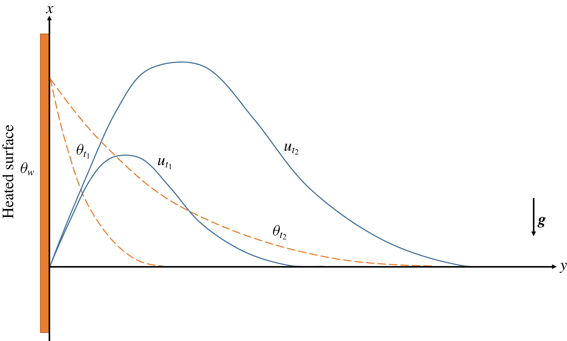
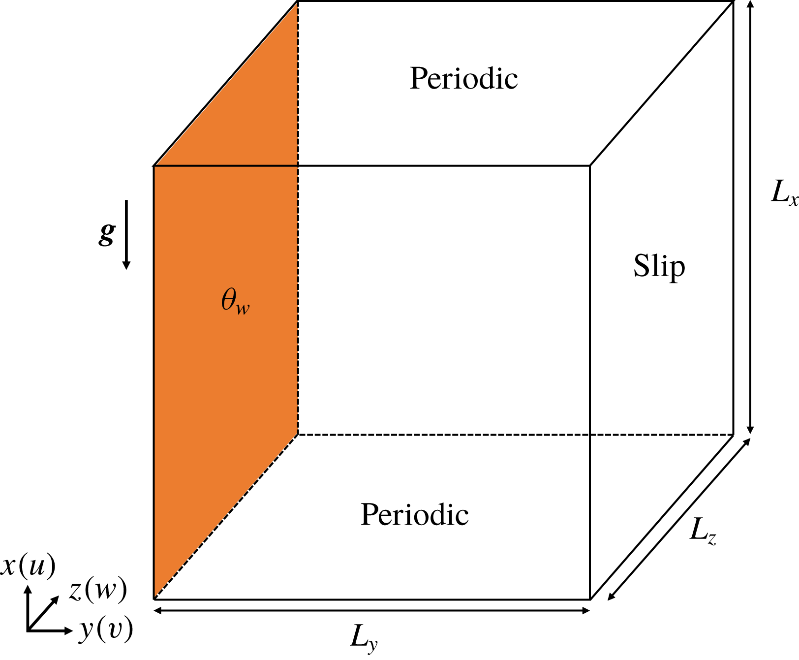
. The gravitational vector
 $\boldsymbol{g}$
is in the negative
 $x$
direction, as depicted in the schematic sketch in figure 1. The Prandtl number is
 $Pr=0.71$
for the problem under consideration. Temperature is made dimensionless with the temperature difference
 $\unicode[STIX]{x0394}T=T_{w}-T_{\infty }$
, i.e.
 $\unicode[STIX]{x1D703}=(T-T_{\infty })/\unicode[STIX]{x0394}T$
. The problem under consideration has no natural length scale as the isothermal wall extends indefinitely in both streamwise (
 $x$
) and spanwise (
 $z$
) directions. The intrinsic length scale
 $L_{s}=\unicode[STIX]{x1D705}^{2/3}/(g\unicode[STIX]{x1D6FD}\unicode[STIX]{x0394}T)^{1/3}$
, time scale
 $t_{s}=\unicode[STIX]{x1D705}^{1/3}/(g\unicode[STIX]{x1D6FD}\unicode[STIX]{x0394}T)^{2/3}$
and velocity scale
 $U_{s}=(\unicode[STIX]{x1D705}g\unicode[STIX]{x1D6FD}\unicode[STIX]{x0394}T)^{1/3}$
are therefore employed to make the other terms dimensionless in equation (2.1) accordingly.
The development of the unsteady natural convection boundary layer profiles (dimensionless streamwise velocity
 $u$
in solid lines and temperature
 $\unicode[STIX]{x1D703}$
in dashed lines) at two different time instants
 $t_{1}$
and
 $t_{2}$
, with
 $t_{2}>t_{1}$
.

2.2 Linearized disturbance equations
We initially examine the characteristics of the two-dimensional linearized system. Two-dimensional perturbations (
 $\tilde{u} ,\tilde{v},\tilde{p},\tilde{\unicode[STIX]{x1D703}}$
) are superimposed upon the flow system by substituting
 $u=U_{b}+\tilde{u}$
,
 $v=\tilde{v}$
,
 $p=p_{b}+\tilde{p}$
,
 $\unicode[STIX]{x1D703}=\unicode[STIX]{x1D703}_{b}+\tilde{\unicode[STIX]{x1D703}}$
into the governing equation (2.1), where the subscript
 $b$
denotes the instantaneous base flow profiles. After omitting the time variation in the base flow and higher-order nonlinear terms, the dimensionless linearized disturbance equations (LDE) are obtained as
 $$\begin{eqnarray}\displaystyle & \displaystyle \frac{\unicode[STIX]{x2202}\tilde{u} }{\unicode[STIX]{x2202}x}+\frac{\unicode[STIX]{x2202}\tilde{v}}{\unicode[STIX]{x2202}y}=0, & \displaystyle\end{eqnarray}$$
 $$\begin{eqnarray}\displaystyle & \displaystyle \frac{\unicode[STIX]{x2202}\tilde{u} }{\unicode[STIX]{x2202}t}+U_{b}\frac{\unicode[STIX]{x2202}\tilde{u} }{\unicode[STIX]{x2202}x}+\tilde{v}\frac{\unicode[STIX]{x2202}U_{b}}{\unicode[STIX]{x2202}y}=-\frac{\unicode[STIX]{x2202}\tilde{p}}{\unicode[STIX]{x2202}x}+Pr\left(\frac{\unicode[STIX]{x2202}^{2}\tilde{u} }{\unicode[STIX]{x2202}x^{2}}+\frac{\unicode[STIX]{x2202}^{2}\tilde{u} }{\unicode[STIX]{x2202}y^{2}}\right)+\tilde{\unicode[STIX]{x1D703}}, & \displaystyle\end{eqnarray}$$
 $$\begin{eqnarray}\displaystyle & \displaystyle \frac{\unicode[STIX]{x2202}\tilde{v}}{\unicode[STIX]{x2202}t}+U_{b}\frac{\unicode[STIX]{x2202}\tilde{v}}{\unicode[STIX]{x2202}x}=-\frac{\unicode[STIX]{x2202}\tilde{p}}{\unicode[STIX]{x2202}y}+Pr\left(\frac{\unicode[STIX]{x2202}^{2}\tilde{v}}{\unicode[STIX]{x2202}x^{2}}+\frac{\unicode[STIX]{x2202}^{2}\tilde{v}}{\unicode[STIX]{x2202}y^{2}}\right), & \displaystyle\end{eqnarray}$$
 $$\begin{eqnarray}\displaystyle & \displaystyle \frac{\unicode[STIX]{x2202}\tilde{\unicode[STIX]{x1D703}}}{\unicode[STIX]{x2202}t}+U_{b}\frac{\unicode[STIX]{x2202}\tilde{\unicode[STIX]{x1D703}}}{\unicode[STIX]{x2202}x}+\tilde{v}\frac{\unicode[STIX]{x2202}\unicode[STIX]{x1D703}_{b}}{\unicode[STIX]{x2202}y}=\frac{\unicode[STIX]{x2202}^{2}\tilde{\unicode[STIX]{x1D703}}}{\unicode[STIX]{x2202}x^{2}}+\frac{\unicode[STIX]{x2202}^{2}\tilde{\unicode[STIX]{x1D703}}}{\unicode[STIX]{x2202}y^{2}}. & \displaystyle\end{eqnarray}$$
The base flow profiles
 $U_{b}$
and
 $\unicode[STIX]{x1D703}_{b}$
are prescribed by the laminar analytical solution to the flow system (2.1), given by Illingworth (Reference Illingworth1950) and Schetz & Eichhorn (Reference Schetz and Eichhorn1962) at some desired
 $t$
or
 $Gr_{\unicode[STIX]{x1D6FF}}$
. For
 $Pr\neq 1$
, the analytical solution can be expressed in the dimensionless form
 $$\begin{eqnarray}\displaystyle & \displaystyle \unicode[STIX]{x1D703}_{b}(\unicode[STIX]{x1D702})=\text{erfc}(\unicode[STIX]{x1D702}), & \displaystyle\end{eqnarray}$$
 $$\begin{eqnarray}\displaystyle & \displaystyle U_{b}(\unicode[STIX]{x1D702},t)=\frac{4t}{1-Pr}\left[\text{i}^{2}\text{erfc}(\unicode[STIX]{x1D702})-\text{i}^{2}\text{erfc}\left(\frac{\unicode[STIX]{x1D702}}{\sqrt{Pr}}\right)\right], & \displaystyle\end{eqnarray}$$
 $\unicode[STIX]{x1D702}=y/2\sqrt{t}$
is a similarity parameter,
 $\text{erf}(\unicode[STIX]{x1D702})$
is the error function of
 $\unicode[STIX]{x1D702}$
,
 $\text{erfc}(\unicode[STIX]{x1D702})=1-\text{erf}(\unicode[STIX]{x1D702})$
is the complementary error function and
 $\text{i}^{n}\text{erfc}(\unicode[STIX]{x1D702})$
is the
 $n$
th integral of the complementary error function,
 $\text{ierfc}(\unicode[STIX]{x1D702})=\exp (-\unicode[STIX]{x1D702}^{2})/\sqrt{\unicode[STIX]{x03C0}}-\unicode[STIX]{x1D702}\text{erfc}(\unicode[STIX]{x1D702})$
and
 $\text{i}^{2}\text{erfc}(\unicode[STIX]{x1D702})=(\text{erfc}(\unicode[STIX]{x1D702})-2\unicode[STIX]{x1D702}\text{ierfc}(\unicode[STIX]{x1D702}))/4$
. In the present study, the boundary layer thickness
 $\unicode[STIX]{x1D6FF}$
is defined by the integral of the velocity profile over the maximum velocity
 $U_{m}$
 $$\begin{eqnarray}\unicode[STIX]{x1D6FF}\equiv \int _{0}^{\infty }\frac{u}{U_{m}}\,\text{d}y,\end{eqnarray}$$
and
 $Gr_{\unicode[STIX]{x1D6FF}}\equiv g\unicode[STIX]{x1D6FD}\unicode[STIX]{x0394}T\unicode[STIX]{x1D6FF}^{3}/\unicode[STIX]{x1D708}^{2}$
denotes the Grashof number based on the velocity integral boundary layer thickness
 $\unicode[STIX]{x1D6FF}$
. From equation (2.3), the two-dimensional solution depends on time
 $t$
and is independent of streamwise coordinate
 $x$
. Since the unsteady temporally developing flow is parallel to the heated surface, the velocity integral boundary layer thickness
 $\unicode[STIX]{x1D6FF}$
as well as the Grashof number
 $Gr_{\unicode[STIX]{x1D6FF}}$
vary with the dimensionless time
 $t$
only.
3 Eigenvalue results
3.1 Quasi-steady approximation
Eigenvalue analysis is commonly used to analyse the linear stability of steady base flows. To obtain an exponential disturbance growth, a steady base flow profile (constant
 $U_{b}$
and
 $\unicode[STIX]{x1D703}_{b}$
in the disturbance equations (2.2)) is required. In the present study, the base flow is ‘frozen’ at some arbitrary dimensionless time
 $t$
so that a steady base flow profile is obtained.
Since the thermal boundary layer of the base flow has a length scale of
 $t^{1/2}$
depending on the dimensionless time
 $t$
(Patterson & Imberger Reference Patterson and Imberger1980), the base flow boundary layer evolves with a time scale of
 $$\begin{eqnarray}\left(\frac{1}{t^{1/2}}\frac{\unicode[STIX]{x2202}t^{1/2}}{\unicode[STIX]{x2202}t}\right)^{-1}=2t\end{eqnarray}$$
and the perturbation quantities evolve with a time scale of
 $$\begin{eqnarray}\left(\frac{1}{A_{t}}\frac{\unicode[STIX]{x2202}A_{t}}{\unicode[STIX]{x2202}t}\right)^{-1}=\frac{1}{\unicode[STIX]{x1D70E}_{k}},\end{eqnarray}$$
where
 $A_{t}$
is the amplitude of the perturbation and
 $\unicode[STIX]{x1D70E}_{k}$
denotes the amplification rate of wavenumber
 $k$
. The quasi-steady approximation may be justified by the argument that the time scale of the evolution of the base flow and that of the perturbations are separated, i.e. the perturbations are independent of the time scale of the evolution of the base flow when the time scale ratio
 $2t\unicode[STIX]{x1D70E}_{k}$
is large so that the base flow can be treated as a quasi-steady state.
This quasi-steady approximation for the unsteady temporally developing parallel boundary layer is analogous to the quasi-parallel approximation in the Orr–Sommerfeld equations for the steady spatially developing boundary layers (Gebhart & Mahajan Reference Gebhart and Mahajan1982) and has been applied to the linear stability analyses for a temporally evolving Rayleigh layer problem (Otto Reference Otto1993), an unsteady Stokes layer problem (Wu & Cowley Reference Wu and Cowley1995) and a time-dependent natural convection in a cavity (Brooker et al. Reference Brooker, Patterson, Graham and Schöpf2000) with good accuracy.
3.2 Freezing the base flow
For the problem considered here, it is convenient to introduce a similarity coordinate in order to freeze the base flow
 $$\begin{eqnarray}\displaystyle & \displaystyle \unicode[STIX]{x1D709}=\frac{x}{2\sqrt{t}}, & \displaystyle\end{eqnarray}$$
 $$\begin{eqnarray}\displaystyle & \displaystyle \unicode[STIX]{x1D702}=\frac{y}{2\sqrt{t}}, & \displaystyle\end{eqnarray}$$
 $$\begin{eqnarray}\displaystyle & \displaystyle \unicode[STIX]{x1D70F}={\unicode[STIX]{x1D70F}_{0}}^{1/3}t, & \displaystyle\end{eqnarray}$$
 $\unicode[STIX]{x1D70F}_{0}$
is an arbitrarily chosen constant at which time instant the base flow is ‘frozen’.
Under these coordinates, the analytical laminar solutions (2.3) read
 $$\begin{eqnarray}\displaystyle & \displaystyle \unicode[STIX]{x1D703}_{b}(\unicode[STIX]{x1D702})=\text{erfc}(\unicode[STIX]{x1D702}), & \displaystyle\end{eqnarray}$$
 $$\begin{eqnarray}\displaystyle & \displaystyle U_{b}(\unicode[STIX]{x1D702},\unicode[STIX]{x1D70F})\equiv V_{b}(\unicode[STIX]{x1D702})\frac{\unicode[STIX]{x1D70F}}{{\unicode[STIX]{x1D70F}_{0}}^{1/3}}=\frac{4\unicode[STIX]{x1D70F}}{(1-Pr){\unicode[STIX]{x1D70F}_{0}}^{1/3}}\left[\text{i}^{2}\text{erfc}(\unicode[STIX]{x1D702})-\text{i}^{2}\text{erfc}\left(\frac{\unicode[STIX]{x1D702}}{\sqrt{Pr}}\right)\right], & \displaystyle\end{eqnarray}$$
 $V_{b}$
is a shape function of the velocity profile. As noted above, equation (3.4) indicates a parallel flow (independent of
 $\unicode[STIX]{x1D709}$
) so that the Grashof number
 $Gr_{\unicode[STIX]{x1D6FF}}$
depends on the dimensionless time
 $t$
(or
 $\unicode[STIX]{x1D70F}$
) only.
The velocity perturbations in equation (2.2) can be described by a perturbation stream function
 $\unicode[STIX]{x1D6F9}$
to ensure continuity, from which
 $$\begin{eqnarray}\displaystyle & \displaystyle \tilde{u} \equiv \frac{\unicode[STIX]{x2202}\unicode[STIX]{x1D6F9}}{\unicode[STIX]{x2202}y}=\frac{\unicode[STIX]{x2202}\unicode[STIX]{x1D6F9}}{\unicode[STIX]{x2202}\unicode[STIX]{x1D702}}\frac{\unicode[STIX]{x2202}\unicode[STIX]{x1D702}}{\unicode[STIX]{x2202}y}, & \displaystyle\end{eqnarray}$$
 $$\begin{eqnarray}\displaystyle & \displaystyle \tilde{v}\equiv -\frac{\unicode[STIX]{x2202}\unicode[STIX]{x1D6F9}}{\unicode[STIX]{x2202}x}=-\frac{\unicode[STIX]{x2202}\unicode[STIX]{x1D6F9}}{\unicode[STIX]{x2202}\unicode[STIX]{x1D709}}\frac{\unicode[STIX]{x2202}\unicode[STIX]{x1D709}}{\unicode[STIX]{x2202}x}. & \displaystyle\end{eqnarray}$$
The linear stability equations for the natural convection boundary layer are obtained after taking the out-of-plane component of the curl of the momentum equations (2.2b ) and (2.2c ),
 $$\begin{eqnarray}\displaystyle & \displaystyle \left(\frac{\unicode[STIX]{x2202}}{\unicode[STIX]{x2202}\unicode[STIX]{x1D70F}}-\frac{\unicode[STIX]{x1D709}}{2\unicode[STIX]{x1D70F}}\frac{\unicode[STIX]{x2202}}{\unicode[STIX]{x2202}\unicode[STIX]{x1D709}}-\frac{\unicode[STIX]{x1D702}}{2\unicode[STIX]{x1D70F}}\frac{\unicode[STIX]{x2202}}{\unicode[STIX]{x2202}\unicode[STIX]{x1D702}}\right)\unicode[STIX]{x0394}\unicode[STIX]{x1D6F9}+\frac{\unicode[STIX]{x1D70F}^{1/2}}{2{\unicode[STIX]{x1D70F}_{0}}^{1/2}}\left(V_{b}\frac{\unicode[STIX]{x2202}\unicode[STIX]{x0394}\unicode[STIX]{x1D6F9}}{\unicode[STIX]{x2202}\unicode[STIX]{x1D709}}-{V_{b}}^{\prime \prime }\frac{\unicode[STIX]{x2202}\unicode[STIX]{x1D6F9}}{\unicode[STIX]{x2202}\unicode[STIX]{x1D709}}\right)=\frac{Pr}{4\unicode[STIX]{x1D70F}}\unicode[STIX]{x1D6E5}^{2}\unicode[STIX]{x1D6F9}+\frac{2\unicode[STIX]{x1D70F}^{1/2}}{{\unicode[STIX]{x1D70F}_{0}}^{1/2}}\frac{\unicode[STIX]{x2202}\tilde{\unicode[STIX]{x1D703}}}{\unicode[STIX]{x2202}\unicode[STIX]{x1D702}}, & \displaystyle \nonumber\\ \displaystyle & & \displaystyle\end{eqnarray}$$
 $$\begin{eqnarray}\displaystyle & \displaystyle \left(\frac{\unicode[STIX]{x2202}}{\unicode[STIX]{x2202}\unicode[STIX]{x1D70F}}-\frac{\unicode[STIX]{x1D709}}{2\unicode[STIX]{x1D70F}}\frac{\unicode[STIX]{x2202}}{\unicode[STIX]{x2202}\unicode[STIX]{x1D709}}-\frac{\unicode[STIX]{x1D702}}{2\unicode[STIX]{x1D70F}}\frac{\unicode[STIX]{x2202}}{\unicode[STIX]{x2202}\unicode[STIX]{x1D702}}\right)\tilde{\unicode[STIX]{x1D703}}+\frac{\unicode[STIX]{x1D70F}^{1/2}}{2{\unicode[STIX]{x1D70F}_{0}}^{1/2}}V_{b}\frac{\unicode[STIX]{x2202}\tilde{\unicode[STIX]{x1D703}}}{\unicode[STIX]{x2202}\unicode[STIX]{x1D709}}-\frac{{\unicode[STIX]{x1D703}_{b}}^{\prime }}{4\unicode[STIX]{x1D70F}}\frac{\unicode[STIX]{x2202}\unicode[STIX]{x1D6F9}}{\unicode[STIX]{x2202}\unicode[STIX]{x1D709}}=\frac{1}{4\unicode[STIX]{x1D70F}}\unicode[STIX]{x0394}\tilde{\unicode[STIX]{x1D703}}, & \displaystyle\end{eqnarray}$$
 $^{\prime }$
, denotes differentiation with respect to
 $\unicode[STIX]{x1D702}$
, and
 $$\begin{eqnarray}\unicode[STIX]{x1D6E5}\equiv \frac{\unicode[STIX]{x2202}^{2}}{\unicode[STIX]{x2202}\unicode[STIX]{x1D709}^{2}}+\frac{\unicode[STIX]{x2202}^{2}}{\unicode[STIX]{x2202}\unicode[STIX]{x1D702}^{2}}.\end{eqnarray}$$
For large enough
 $\unicode[STIX]{x1D70F}$
, the first terms in equations (3.6) can be simplified as
 $$\begin{eqnarray}\frac{\unicode[STIX]{x2202}}{\unicode[STIX]{x2202}\unicode[STIX]{x1D70F}}-\frac{\unicode[STIX]{x1D709}}{2\unicode[STIX]{x1D70F}}\frac{\unicode[STIX]{x2202}}{\unicode[STIX]{x2202}\unicode[STIX]{x1D709}}-\frac{\unicode[STIX]{x1D702}}{2\unicode[STIX]{x1D70F}}\frac{\unicode[STIX]{x2202}}{\unicode[STIX]{x2202}\unicode[STIX]{x1D702}}\sim \frac{\unicode[STIX]{x2202}}{\unicode[STIX]{x2202}\unicode[STIX]{x1D70F}}.\end{eqnarray}$$
It is noted that the conduction and viscous terms are retained even though they have the same asymptotic behaviour. Nevertheless, consider the perturbation normal modes given in equation (3.9),
 $$\begin{eqnarray}\unicode[STIX]{x1D6F9}=\unicode[STIX]{x1D713}(\unicode[STIX]{x1D702})\text{e}^{\text{i}\unicode[STIX]{x1D6FC}(\unicode[STIX]{x1D709}-c\unicode[STIX]{x1D70F})},\end{eqnarray}$$
where
 $\text{i}=\sqrt{-1}$
is the imaginary unit,
 $\unicode[STIX]{x1D6FC}=2\sqrt{t}k$
denotes the normalized wavenumber and
 $\unicode[STIX]{x1D713}$
is the amplitude of the stream function. The imaginary part
 $c_{\text{i}}$
of the complex number
 $c=c_{\text{r}}+\text{i}c_{\text{i}}$
determines whether the perturbation wave
 $\unicode[STIX]{x1D6FC}$
will be amplified (
 $c_{\text{i}}>0$
) or damped (
 $c_{\text{i}}<0$
) in time by the base flow, while the real part
 $c_{\text{r}}$
indicates phase speed of the wave
 $\unicode[STIX]{x1D6FC}$
.
The temperature perturbation can also be described in a similar form using the amplitude function of the temperature perturbation
 $s$
as follows:
 $$\begin{eqnarray}\tilde{\unicode[STIX]{x1D703}}=s(\unicode[STIX]{x1D702})\text{e}^{\text{i}\unicode[STIX]{x1D6FC}(\unicode[STIX]{x1D709}-c\unicode[STIX]{x1D70F})}.\end{eqnarray}$$
The flow is then frozen at
 $\unicode[STIX]{x1D70F}=\unicode[STIX]{x1D70F}_{0}$
(so that
 $t_{0}={\unicode[STIX]{x1D70F}_{0}}^{2/3}$
, where
 $t_{0}$
is the dimensionless time instant in the intrinsic scale) after the substitution of equations (3.9) and (3.10) into (3.6). The stability equations are obtained as
 $$\begin{eqnarray}\displaystyle & \displaystyle \text{i}\unicode[STIX]{x1D6FC}\left[\left(\frac{V_{b}}{2}-c\right)(\unicode[STIX]{x1D713}^{\prime \prime }-\unicode[STIX]{x1D6FC}^{2}\unicode[STIX]{x1D713})-\frac{{V_{b}}^{\prime \prime }}{2}\unicode[STIX]{x1D713}\right]=\frac{Pr}{4\unicode[STIX]{x1D70F}_{0}}(\unicode[STIX]{x1D713}^{\prime \prime \prime \prime }-2\unicode[STIX]{x1D6FC}^{2}\unicode[STIX]{x1D713}^{\prime \prime }+\unicode[STIX]{x1D6FC}^{4}\unicode[STIX]{x1D713})+2s^{\prime },\quad & \displaystyle\end{eqnarray}$$
 $$\begin{eqnarray}\displaystyle & \displaystyle \text{i}\unicode[STIX]{x1D6FC}\left[\left(\frac{V_{b}}{2}-c\right)s-\frac{1}{4\unicode[STIX]{x1D70F}_{0}}{\unicode[STIX]{x1D703}_{b}}^{\prime }\unicode[STIX]{x1D713}\right]=\frac{1}{4\unicode[STIX]{x1D70F}_{0}}(s^{\prime \prime }-\unicode[STIX]{x1D6FC}^{2}s). & \displaystyle\end{eqnarray}$$
 $c$
, which permits non-zero solutions for
 $s$
and
 $\unicode[STIX]{x1D713}$
at given positive
 $\unicode[STIX]{x1D6FC}$
and
 $\unicode[STIX]{x1D70F}_{0}$
(equivalently,
 $Gr_{\unicode[STIX]{x1D6FF}}$
), as an eigenvalue problem. The amplification rate in the intrinsic scale is therefore
 $$\begin{eqnarray}\unicode[STIX]{x1D70E}_{k}={\unicode[STIX]{x1D70F}_{0}}^{1/3}\unicode[STIX]{x1D6FC}c_{\text{i}}={t_{0}}^{1/2}\unicode[STIX]{x1D6FC}c_{\text{i}}.\end{eqnarray}$$
For the isothermal vertical wall, the boundary conditions are defined for the perturbations
 $$\begin{eqnarray}\displaystyle & \displaystyle \unicode[STIX]{x1D713}(0)=\unicode[STIX]{x1D713}^{\prime }(0)=s(0)=0, & \displaystyle\end{eqnarray}$$
 $$\begin{eqnarray}\displaystyle & \displaystyle \unicode[STIX]{x1D713}(\infty )=\unicode[STIX]{x1D713}^{\prime }(\infty )=s(\infty )=0. & \displaystyle\end{eqnarray}$$
3.3 Eigenvalue solutions
Solutions to the linear stability equations (3.11) are obtained by solving the eigenvalue problem with varying
 $\unicode[STIX]{x1D70F}_{0}$
and
 $\unicode[STIX]{x1D6FC}$
using the generalized Schur decomposition algorithm (also known as the QZ algorithm). The second-order finite difference method is used to numerically discretize the equations. Implementing the boundary conditions given in (3.13), calculation is carried out in a domain size of
 $0<\unicode[STIX]{x1D702}<10$
with
 $N_{y}=1024$
uniformly distributed nodes. Domain and grid size dependency tests are carried out to ensure a reliable solution.
In order to compare with the direct numerical simulation results, the
 $\unicode[STIX]{x1D70F}_{0}$
-dependent eigenvalue solutions are also presented in terms of
 $Gr_{\unicode[STIX]{x1D6FF}}$
. Here, the boundary layer thickness is given by
 $$\begin{eqnarray}\unicode[STIX]{x1D6FF}\equiv \int _{0}^{\infty }\frac{U_{b}}{U_{m}}\,\text{d}y=\int _{0}^{\infty }\frac{U_{b}}{U_{m}}\,\text{d}\unicode[STIX]{x1D702}\frac{\unicode[STIX]{x2202}y}{\unicode[STIX]{x2202}\unicode[STIX]{x1D702}}=2{\mathcal{C}}{\unicode[STIX]{x1D70F}_{0}}^{1/3},\end{eqnarray}$$
where
 $$\begin{eqnarray}{\mathcal{C}}=\frac{4\displaystyle \int _{0}^{\infty }[\text{i}^{2}\text{erfc}(\unicode[STIX]{x1D702})-\text{i}^{2}\text{erfc}(\unicode[STIX]{x1D702}/\sqrt{Pr})]\,\text{d}\unicode[STIX]{x1D702}}{\text{erfc}(\unicode[STIX]{x1D702}_{m})-\text{erfc}(\unicode[STIX]{x1D702}_{m}/\sqrt{Pr})}\sim 0.855\end{eqnarray}$$
is a constant since the base flow velocity profile
 $U_{b}$
and the maximum velocity
 $U_{m}$
are both linearly proportional to time in the similarity coordinate, and
 $\unicode[STIX]{x1D702}_{m}$
is the maximum velocity location that satisfies
 $$\begin{eqnarray}\sqrt{Pr}\text{ierfc}(\unicode[STIX]{x1D702}_{m})=\text{ierfc}\left(\frac{\unicode[STIX]{x1D702}_{m}}{\sqrt{Pr}}\right).\end{eqnarray}$$
Hence, the Grashof number is given by
 $$\begin{eqnarray}Gr_{\unicode[STIX]{x1D6FF}}=\frac{8{\mathcal{C}}^{3}}{Pr^{2}}\unicode[STIX]{x1D70F}_{0}.\end{eqnarray}$$
The evolution of the base flow boundary layer is therefore slow when compared with the perturbation evolutions when the time scale ratio
 $$\begin{eqnarray}2t\unicode[STIX]{x1D70E}_{k}=2\unicode[STIX]{x1D6FC}c_{\text{i}}\unicode[STIX]{x1D70F}_{0}\sim O(Gr_{\unicode[STIX]{x1D6FF}})\end{eqnarray}$$
is large enough.
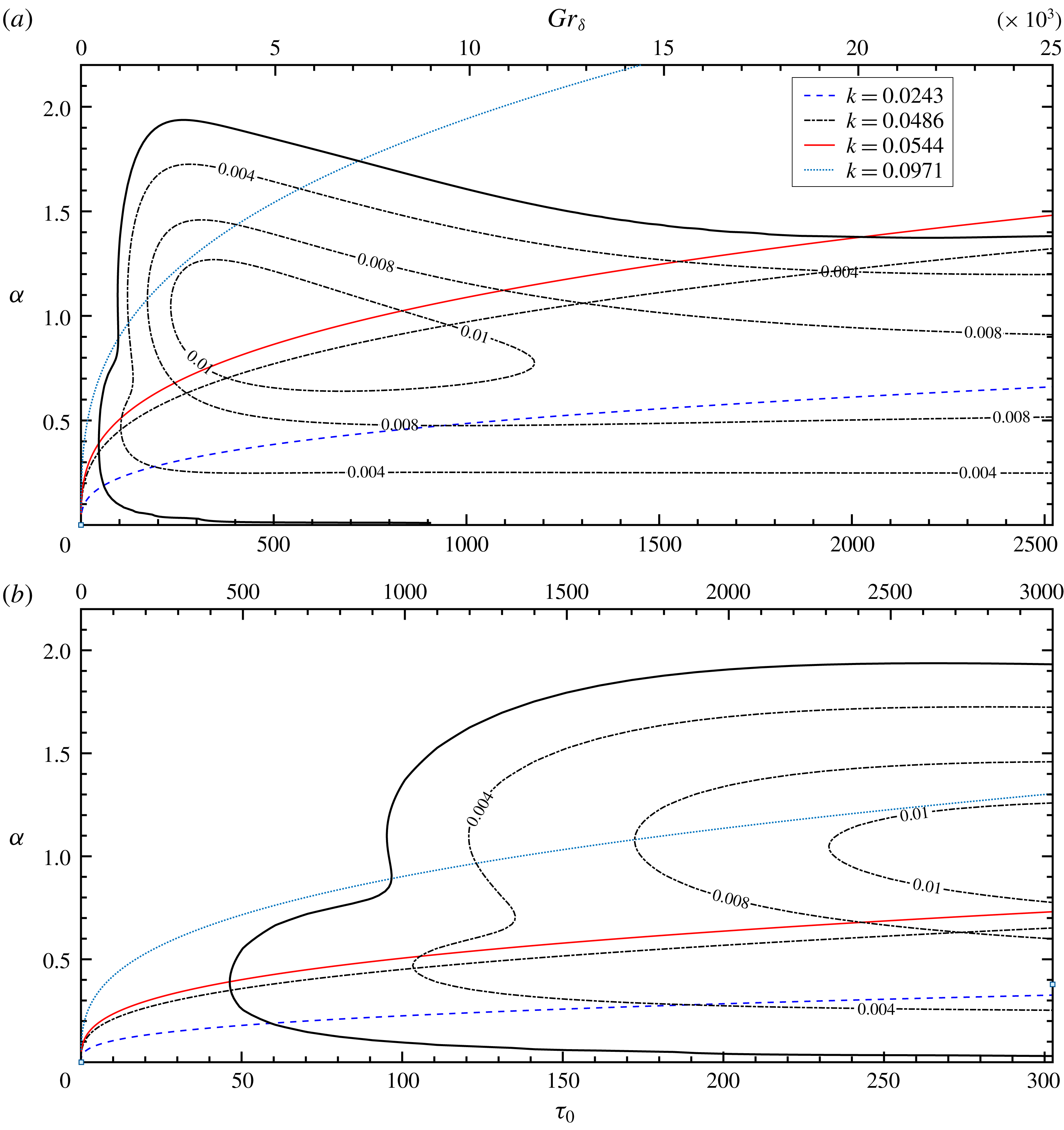
Linear stability margin of the temporally evolving NCBL for
 $Pr=0.71$
; (a) marginal stability plane; (b) enlarged near the critical point; (black solid) neutral curve, where
 $\unicode[STIX]{x1D6FC}c_{\text{i}}=0$
; (dash-dotted contours) constant amplification rate
 $\unicode[STIX]{x1D6FC}c_{\text{i}}=0.004$
,
 $\unicode[STIX]{x1D6FC}c_{\text{i}}=0.008$
, and
 $\unicode[STIX]{x1D6FC}c_{\text{i}}=0.01$
; with constant wavenumber
 $k$
trajectories in the marginal stability plane, (blue dashed)
 $k=0.0243$
; (black dash-dotted)
 $k=0.0486$
; (red solid)
 $k=0.0544$
; (turquoise dotted)
 $k=0.0971$
.

The resulting stability margin for
 $Pr=0.71$
is shown in figure 2 with the trajectories of the constant wavenumber
 $k$
. It shows that the base flow at given
 $Gr_{\unicode[STIX]{x1D6FF}}$
is unstable to a range of wavenumbers and selectively amplifies the perturbations, similarly to the spatially developing cases in Mahajan & Gebhart (Reference Mahajan and Gebhart1979) and Qureshi & Gebhart (Reference Qureshi and Gebhart1978). The maximum amplification rates (
 $\unicode[STIX]{x1D6FC}c_{\text{i}}\geqslant 0.01$
) can be found in a core region between
 $Gr_{\unicode[STIX]{x1D6FF}}\sim 2300$
and
 $Gr_{\unicode[STIX]{x1D6FF}}\sim 11\,700$
for a small band of frequencies from
 $k\sim 0.0337$
to
 $k\sim 0.0950$
.
The critical point, that is the minimum
 $\unicode[STIX]{x1D70F}_{0}$
at which the base flow is linearly unstable, and the corresponding wavenumber and phase velocity are
 $\unicode[STIX]{x1D70F}_{0}=45.7978$
,
 $\unicode[STIX]{x1D6FC}=0.3894$
and
 $c=c_{\text{r}}=0.1193$
in the similarity coordinate, or more generally
 $$\begin{eqnarray}\displaystyle Gr_{\unicode[STIX]{x1D6FF}}=454.2,\quad k=0.0544,\quad U_{p}=3.0551, & & \displaystyle\end{eqnarray}$$
where
 $U_{p}=2{\unicode[STIX]{x1D70F}_{0}}^{2/3}c_{\text{r}}$
. It is interesting to find that at the critical point, the phase speed of the most unstable wavenumber
 $U_{p}$
equals the maximum streamwise velocity
 $U_{m}$
in the temporally evolving NCBL. This is consistent with the observations of Armfield & Patterson (Reference Armfield and Patterson1992).
On the other hand, Nachtsheim (Reference Nachtsheim1963) reported a much higher critical point,
 $Gr_{\unicode[STIX]{x1D6FF}}=642.9$
and
 $k=0.0529$
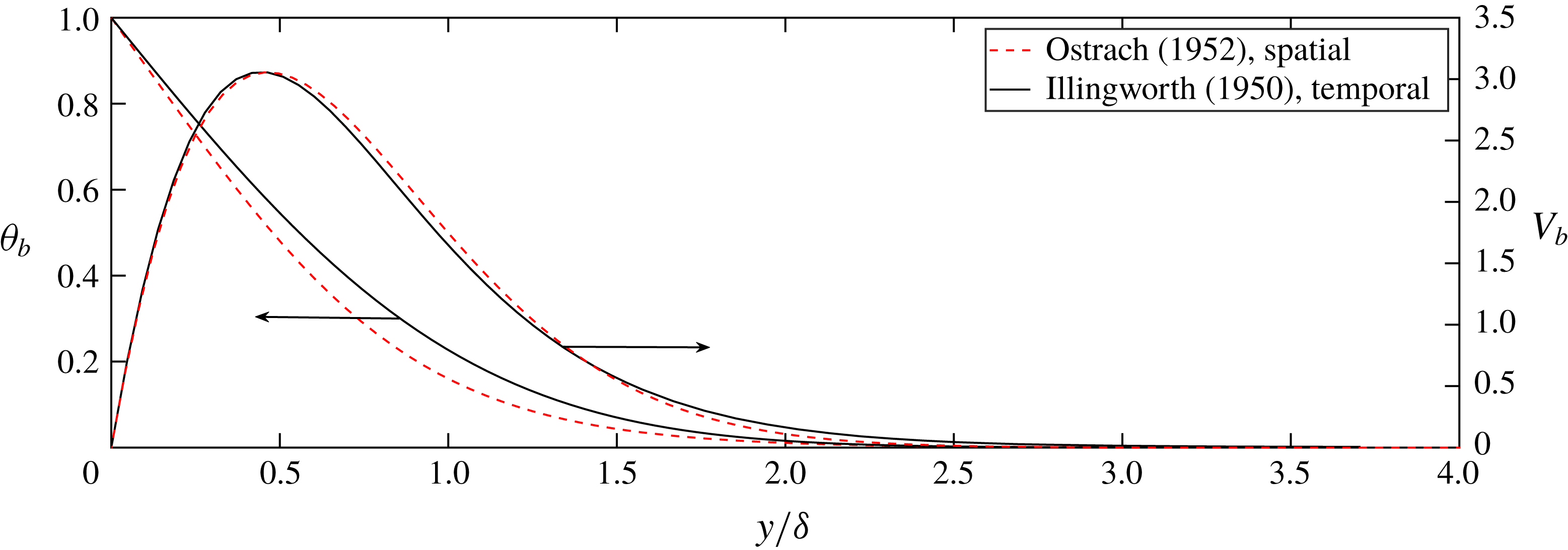
, for a spatially developing NCBL. The steady, spatially developing base flow was given by the similarity numerical solution of Ostrach (Reference Ostrach1952) and in their analysis parallel flow was assumed. In contrast, the base flow in the present study is indeed a parallel flow and the unsteadiness is treated by freezing the profile in the similarity coordinate. It is evident that the discrepancy in the critical point is due to the difference in the shape functions of the base flow profiles for the two NCBL flows, as depicted in figure 3.
Shape function of the base flow temperature profile (left) and velocity profile (right) for a spatially developing NCBL (Ostrach Reference Ostrach1952) (dashed lines); and a temporally evolving NCBL (Illingworth Reference Illingworth1950; Schetz & Eichhorn Reference Schetz and Eichhorn1962) (solid lines).

In figure 2(a), the trajectory of the constant wavenumber at
 $k=0.0971$
intersects the neutral curve at
 $Gr_{\unicode[STIX]{x1D6FF}}\sim 950$
and
 $Gr_{\unicode[STIX]{x1D6FF}}\sim 7000$
. This suggests the discrete mode (
 $k=0.0971$
) follows a ‘damped–amplified–damped’ pathway, i.e. the disturbance wave first starts to be amplified at about
 $Gr_{\unicode[STIX]{x1D6FF}}\sim 950$
, and is later damped from
 $Gr_{\unicode[STIX]{x1D6FF}}\sim 7000$
. Similar behaviour can be found for the most unstable wavenumber
 $k=0.0544$
towards
 $Gr_{\unicode[STIX]{x1D6FF}}\sim 20\,000$
. In contrast to the spatial cases (Dring & Gebhart Reference Dring and Gebhart1968, Reference Dring and Gebhart1969), the wavenumber which receives the maximum total amplification
 $\unicode[STIX]{x1D70D}_{max}$
is not necessarily higher than the most unstable frequency at the critical point (in this case
 $k=0.0544$
), but is dependent on the pathway through the marginal stability map in figure 2. The total amplification is defined by equation (3.20) as follows:
 $$\begin{eqnarray}\unicode[STIX]{x1D70D}_{k}=\int _{Gr_{\unicode[STIX]{x1D6FF}_{1}}}^{Gr_{\unicode[STIX]{x1D6FF}_{2}}}\unicode[STIX]{x1D70E}_{k}(k,Gr_{\unicode[STIX]{x1D6FF}})\,\text{d}t.\end{eqnarray}$$
Here,
 $\unicode[STIX]{x1D70D}_{k}$
represents the total amplification of wavenumber
 $k$
from
 $Gr_{\unicode[STIX]{x1D6FF}_{1}}$
to
 $Gr_{\unicode[STIX]{x1D6FF}_{2}}$
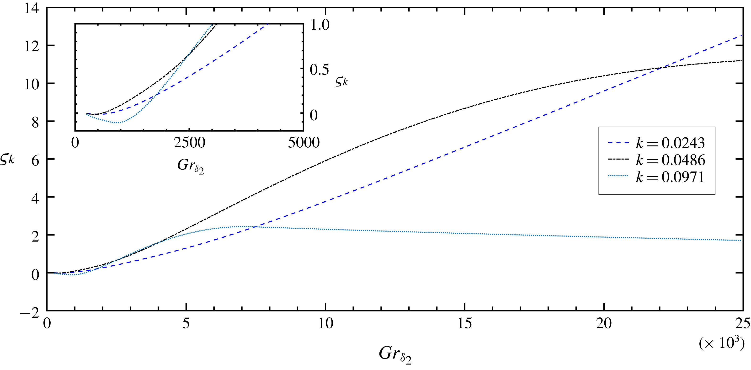
. Figure 4 depicts the total amplification of perturbation modes at
 $k=0.0243$
,
 $k=0.0486$
and
 $k=0.0971$
with a fixed starting point of
 $Gr_{\unicode[STIX]{x1D6FF}_{1}}=250$
. The discrete mode
 $k=0.0486$
first becomes unstable to the base flow and receives the most amplification among the three modes up to
 $Gr_{\unicode[STIX]{x1D6FF}_{2}}\sim 2500$
. After this range, the total amplification of the discrete mode
 $k=0.0971$
outgrows that of
 $k=0.0486$
for a short period. The most amplified frequency later switches back to
 $k=0.0486$
since the instantaneous amplification rate of
 $k=0.0971$
starts to drop at
 $Gr_{\unicode[STIX]{x1D6FF}_{2}}\sim 3500$
, as indicated by figure 2. At about
 $Gr_{\unicode[STIX]{x1D6FF}_{2}}\sim 7000$
, the total amplification of
 $k=0.0971$
starts to decrease as the instantaneous amplification rate is negative (i.e. perturbation experiences damping).
Total amplification of discrete modes of
 $k=0.0243$
(blue dashed),
 $k=0.0486$
(black dash-dotted) and
 $k=0.0971$
(turquoise dotted), with
 $Gr_{\unicode[STIX]{x1D6FF}_{1}}=250$
; Inset shows
 $\unicode[STIX]{x1D70D}_{k}$
at small
 $Gr_{\unicode[STIX]{x1D6FF}_{2}}$
.

4 Direct solution of the LDE with ‘frozen’ base flow
4.1 Initial-value problem on two-dimensional frozen base flow
The linear stability properties of the temporally evolving flow may also be obtained by a full solution of the perturbation equations. The linearized disturbance equations (2.2) are spatially discretized using the finite volume method. The nonlinear advection terms are discretized by a fourth-order scheme, whilst all other spatial terms are second-order accurate. The second-order Adams–Bashforth method is adopted as the time stepping scheme with the Crank–Nicolson method used for the diffusive terms. The code has been extensively validated in a number of the natural convection problems (Williamson, Armfield & Kirkpatrick Reference Williamson, Armfield and Kirkpatrick2012; Williamson et al. Reference Williamson, Armfield, Lin and Kirkpatrick2016).
The streamwise (
 $x$
) boundaries are made periodic to eliminate the leading edge effect so that a temporally evolving flow is obtained. The velocity and the temperature perturbations are restricted by the non-slip and non-permeability boundary conditions on the isothermal wall (
 $\tilde{u} =\tilde{v}=\tilde{\unicode[STIX]{x1D703}}=0$
at
 $y=0$
). In the far field, both velocity and temperature perturbation decay, i.e.
 $\tilde{u} =\tilde{v}=\tilde{\unicode[STIX]{x1D703}}=0$
at
 $y=L_{y}$
. A schematic diagram of the simulation domain is shown in figure 5.
The computational domain and coordinates for the direct numerical simulations, the vertical isothermal wall is coloured in orange.

The base flow profiles
 $U_{b}$
and
 $\unicode[STIX]{x1D703}_{b}$
are obtained as the laminar analytical solutions given by equation (2.3) at some desired base flow boundary layer Grashof number
 $Gr_{\unicode[STIX]{x1D6FF}_{0}}$
. To investigate the stability properties of the flow, the initialized base laminar boundary layer is augmented with a streamwise temperature perturbation that decays in the wall-normal direction
 $$\begin{eqnarray}\tilde{\unicode[STIX]{x1D703}}_{n}=\unicode[STIX]{x1D703}_{b}(y)A_{n}\sin \left(2\unicode[STIX]{x03C0}n\frac{x}{L_{x}}\right),\end{eqnarray}$$
where
 $n$
is a real positive integer indicating the mode number (
 $n/L_{x}$
) and the wavenumber (
 $k=2\unicode[STIX]{x03C0}n/L_{x}$
) of the sinusoidal perturbation. The amplitude of the temperature perturbation
 $A_{n}$
is selected so that the perturbation interacts with the base flow linearly, i.e. the amplification rate of the perturbation is independent of
 $A_{n}$
. In the present study, it is chosen as
 $A_{n}=10^{-3}$
. It is noted that in contrast to some numerical studies (Abedin, Tsuji & Hattori Reference Abedin, Tsuji and Hattori2009; Nakao, Hattori & Suto Reference Nakao, Hattori and Suto2017), there is no velocity perturbation added to the flow as the velocity field is coupled to the temperature field and will respond directly to the temperature perturbation while remaining divergence free. A similar technique was also employed by Janssen & Armfield (Reference Janssen and Armfield1996) and Zhao, Lei & Patterson (Reference Zhao, Lei and Patterson2017) for NCBL flows.
The instantaneous linear stability of the unsteady flow is examined by integrating the linearized disturbance equations (2.2) for choices of perturbation wavenumber
 $k$
in time for a ‘frozen’ (steady) base flow at time
 $t$
(which is equivalent to the Grashof number based on the base flow boundary layer thickness
 $Gr_{\unicode[STIX]{x1D6FF}}$
) as an initial-value problem.
4.2 Solutions of the linearized disturbance equations
The two-dimensional solutions of the disturbance equations are numerically obtained in a domain of
 $L_{x}\times L_{y}=1035\times 1035$
with a
 $N_{x}\times N_{y}=1024\times 1024$
Cartesian grid. The grid is uniform in the streamwise (
 $x$
) direction, but is geometrically stretched with a maximum stretching rate of
 $\unicode[STIX]{x1D6FE}=1.24\,\%$
in the wall-normal (
 $y$
) direction. Additional simulations varying the domain size and the grid size were undertaken to ensure the solution is not adversely affected by the numerical settings.
The initial-value problem is investigated by monitoring the time traces of the perturbation quantities
 $\tilde{\unicode[STIX]{x1D703}}$
and
 $\tilde{u}$
at an arbitrary fixed point (
 $x_{p}$
,
 $y_{p}$
) within the boundary layer. Given the base flow profiles
 $U_{b}$
and
 $\unicode[STIX]{x1D703}_{b}$
at some instantaneous base flow
 $Gr_{\unicode[STIX]{x1D6FF}_{0}}$
, the flow is unstable to the perturbation of wavenumber
 $k$
if the amplitude of the perturbation grows with time. Here, the subscript
 $0$
indicates the initialization quantities.
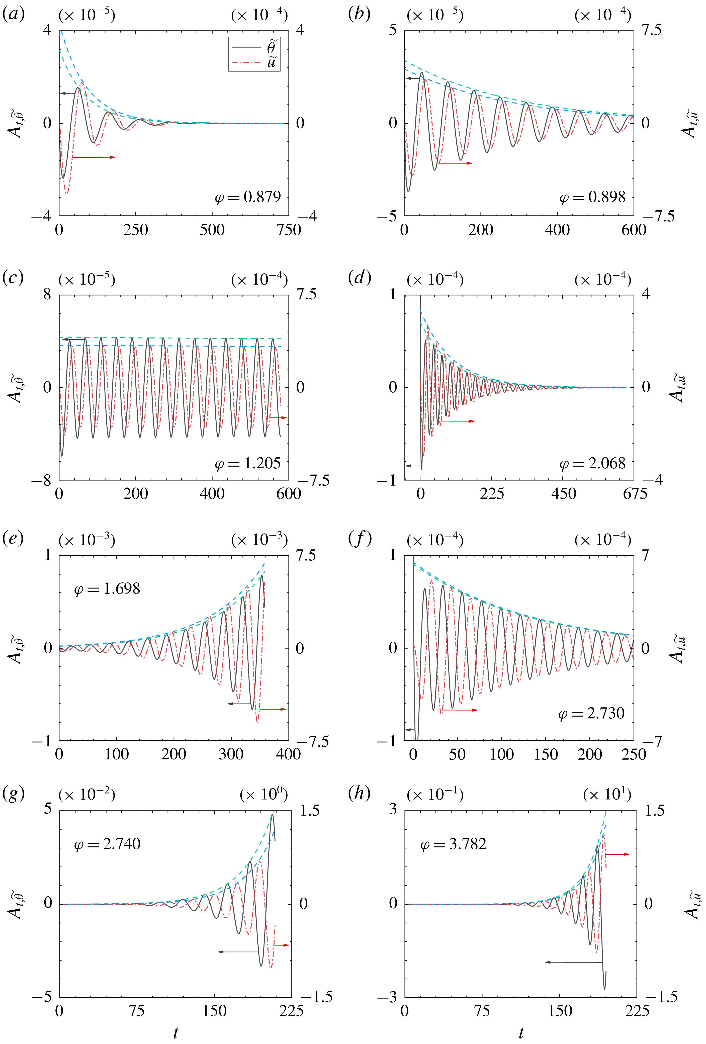
Time traces of the velocity and temperature perturbations
 $\tilde{\unicode[STIX]{x1D703}}$
(black solid),
 $\tilde{u}$
(red dash-dotted) at location
 $(x_{p},y_{p})=(647.6,0.2)$
for (a) base flow at
 $Gr_{\unicode[STIX]{x1D6FF}_{0}}=249.3$
and
 $k=0.0243$
(
 $n=4$
); (b) base flow at
 $Gr_{\unicode[STIX]{x1D6FF}_{0}}=454.3$
and
 $k=0.0243$
(
 $n=4$
); (c) base flow at
 $Gr_{\unicode[STIX]{x1D6FF}_{0}}=454.3$
and
 $k=0.0486$
(
 $n=8$
); (d) base flow at
 $Gr_{\unicode[STIX]{x1D6FF}_{0}}=454.3$
and
 $k=0.0971$
(
 $n=16$
); (e) base flow at
 $Gr_{\unicode[STIX]{x1D6FF}_{0}}=704.3$
and
 $k=0.0486$
(
 $n=8$
); (f) base flow at
 $Gr_{\unicode[STIX]{x1D6FF}_{0}}=704.3$
and
 $k=0.0971$
(
 $n=16$
); (g) base flow at
 $Gr_{\unicode[STIX]{x1D6FF}_{0}}=1992.1$
and
 $k=0.0486$
(
 $n=8$
); (h) base flow at
 $Gr_{\unicode[STIX]{x1D6FF}_{0}}=1992.1$
and
 $k=0.0971$
(
 $n=16$
); exponential envelopes of the signals (dashed lines).

The time traces in figure 6 show that the velocity perturbation lags the temperature perturbation by a constant phase difference, and the phase lag
 $\unicode[STIX]{x1D711}$
increases with wavenumber
 $k$
and the base flow Grashof number
 $Gr_{\unicode[STIX]{x1D6FF}_{0}}$
. The envelopes of the perturbation signals of wavenumber
 $k$
should follow the exponential growth
 $A_{n}e^{\unicode[STIX]{x1D70E}_{k}t}$
(or decay, depending on the sign of
 $\unicode[STIX]{x1D70E}_{k}$
) in time. The amplification rate
 $\unicode[STIX]{x1D70E}_{k}$
is defined by
 $$\begin{eqnarray}\unicode[STIX]{x1D70E}_{k}\equiv \frac{1}{A_{t}}\frac{\unicode[STIX]{x2202}A_{t}}{\unicode[STIX]{x2202}t},\end{eqnarray}$$
where the instantaneous perturbation amplitudes
 $A_{t}$
, at time
 $t$
, of the solutions to the linearized disturbance equations (2.2) are obtained by taking the fast Fourier transform in the streamwise (
 $x$
) direction of the perturbation quantities
 $\tilde{\unicode[STIX]{x1D703}}$
and
 $\tilde{u}$
at
 $y=y_{p}$
. The development of
 $A_{t}$
is depicted at four instances in figure 7, showing the temporal responses of the normal modes at different
 $Gr_{\unicode[STIX]{x1D6FF}_{0}}$
.
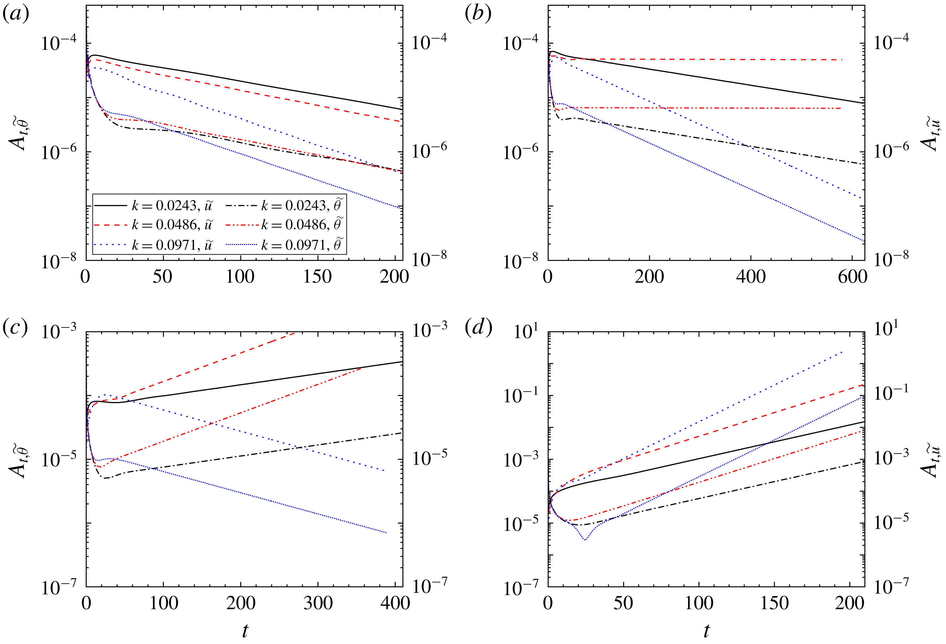
Time traces of the velocity and temperature perturbation amplitudes
 $A_{t,\tilde{u} }$
and
 $A_{t,\tilde{\unicode[STIX]{x1D703}}}$
at
 $y=y_{p}=0.2$
, ‘frozen’ base flow at (a)
 $Gr_{\unicode[STIX]{x1D6FF}_{0}}=249.3$
; (b)
 $Gr_{\unicode[STIX]{x1D6FF}_{0}}=454.3$
; (c)
 $Gr_{\unicode[STIX]{x1D6FF}_{0}}=704.3$
; (d)
 $Gr_{\unicode[STIX]{x1D6FF}_{0}}=1992.1$
.

From figure 7, it is clear that the velocity and temperature perturbations share the same exponential slope, such that
 $$\begin{eqnarray}\unicode[STIX]{x1D70E}_{k,\tilde{u} }=\unicode[STIX]{x1D70E}_{k,\tilde{\unicode[STIX]{x1D703}}}=\unicode[STIX]{x1D70E}_{k}\end{eqnarray}$$
for all
 $k$
cases in the linear stage of the steady base flow. The normal modes are damped at small
 $Gr_{\unicode[STIX]{x1D6FF}_{0}}$
, as shown in figures 6(a) and 7(a). The laminar base flow is then filtering for a specific marginally unstable wavenumber (
 $\unicode[STIX]{x1D70E}_{k}=-0.0001$
, see
 $k=0.0486$
in (c) where the envelope is almost horizontal) at critical
 $Gr_{\unicode[STIX]{x1D6FF}}$
. With increasing
 $Gr_{\unicode[STIX]{x1D6FF}}$
, the range of discrete modes that are unstable to the base flow are broadened until all modes shown are amplified (
 $\unicode[STIX]{x1D70E}_{k}>0$
) by the base flow at different rates at
 $Gr_{\unicode[STIX]{x1D6FF}_{0}}=1992.1$
.
It is worth noting that there is always a region where the amplitude of the perturbation does not follow the linear growth/decay immediately after the disturbance is introduced into the base flow. This process, also known as receptivity, tunes the artificial perturbation to an appropriate initial amplitude and phase condition as the boundary layer receives the external disturbance (Morkovin Reference Morkovin1969; Reed, Saric & Arnal Reference Reed, Saric and Arnal1996; Saric, Reed & Kerschen Reference Saric, Reed and Kerschen2002). The details of the receptivity process, however, are beyond the scope of the present study. We shall only focus on the flow stability after the receptivity.
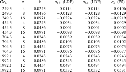
The detailed linear stability solutions to the ‘frozen’ base flows at given pairs of
 $Gr_{\unicode[STIX]{x1D6FF}_{0}}$
and
 $k$
are tabulated in table 1. Both linearized disturbance solutions and eigenvalue calculations are in good agreement.
Amplification rate
 $\unicode[STIX]{x1D70E}_{k}$
for
 $\tilde{\unicode[STIX]{x1D703}}$
and
 $\tilde{u}$
signals at given pairs of
 $Gr_{\unicode[STIX]{x1D6FF}}$
and
 $k$
; linearized disturbance equations; eigenvalue solutions (ES).

5 Direct numerical simulation (DNS)
5.1 Direct stability analysis using the full Navier–Stokes equations
Using the same numerical techniques in § 4, the full Navier–Stokes equations (2.1) are numerically solved in both two-dimensional and three-dimensional forms to incorporate the effects of the temporally evolving base flow and of nonlinearity on flow stability.
The boundary conditions for the velocity and temperature fields are the non-slip and isothermal non-permeable wall, i.e.
 $u=v=w=0$
and
 $\unicode[STIX]{x1D703}_{w}=1$
at
 $y=0$
and the slip wall condition in the far field, i.e.
 $\unicode[STIX]{x2202}u/\unicode[STIX]{x2202}y=\unicode[STIX]{x1D703}=0$
at
 $y=L_{y}$
. Periodic boundaries are imposed in streamwise and spanwise directions to allow a temporally evolving flow. Temporal responses of the perturbation waves are monitored and compared with the instantaneous linear stability solutions to address the unsteady effect of the base flow.
Simulation settings of the direct stability analyses; (
 $^{\ast }$
) both velocity and temperature fields are perturbed by pre-tuned perturbations from the linearized disturbance equations.

5.2 Direct numerical simulation results
The direct numerical calculations are carried out in a domain of
 $L_{x}\times L_{y}(\times L_{z})=1035\times 1035(\times 1035)$
with a non-staggered Cartesian grid. The grid is uniform in the streamwise (
 $x$
) and spanwise (
 $z$
) directions, but is geometrically stretched with a maximum stretching rate of
 $\unicode[STIX]{x1D6FE}$
in the wall-normal (
 $y$
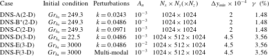
) direction. Simulation settings are listed in table 2. To minimize the extent of the receptivity process, in the DNS-B case both the temperature and velocity fields are perturbed with ‘pre-tuned’ perturbations from the linearized ‘frozen base flow’ simulation. For the two-dimensional simulation, temperature perturbations in the form of equation (4.1) are examined individually by looking at the temporal responses after feeding the discrete modes (initial perturbations) into the prescribed laminar base flow. In the present study, the two-dimensional simulations are initialized at
 $Gr_{\unicode[STIX]{x1D6FF}_{0}}=249.3$
with discrete perturbation modes of
 $k=0.0243$
,
 $k=0.0486$
, and
 $k=0.0971$
. As the base flow profiles
 $\unicode[STIX]{x1D703}_{b}$
and
 $U_{b}$
follow the laminar analytical solution (2.3), the perturbation quantities are found to be
 $\tilde{\unicode[STIX]{x1D703}}=\unicode[STIX]{x1D703}-\unicode[STIX]{x1D703}_{b}$
and
 $\tilde{u} =u-U_{b}$
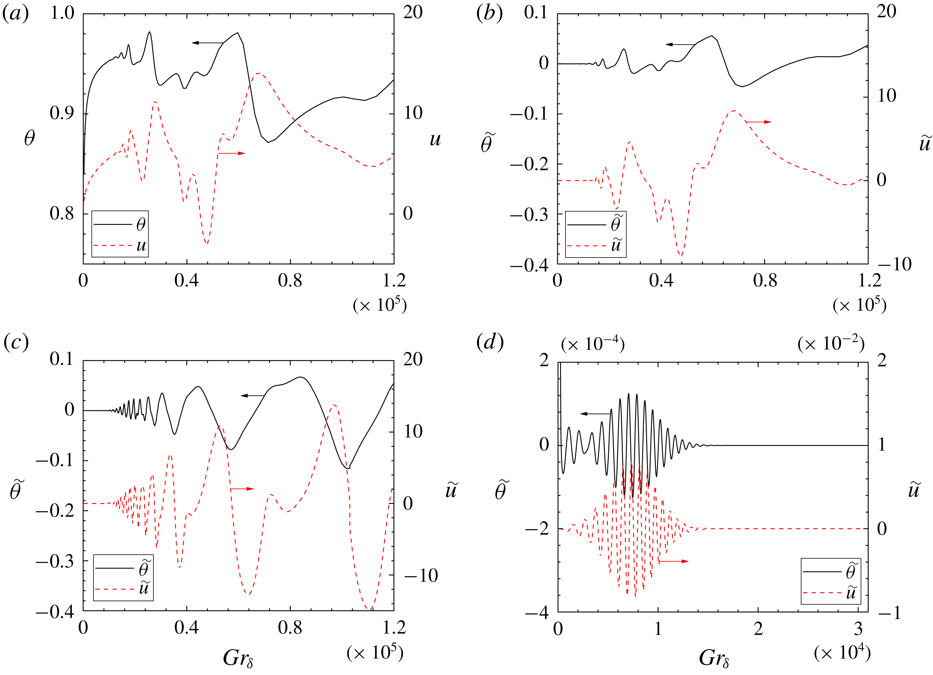
. The resultant time traces show that the discrete modes
 $k=0.0243$
and
 $k=0.0486$
, figure 8(a–c), are amplified with time by the evolving base flow, whereas the perturbation at
 $k=0.0971$
, figure 8(d), is damped out at about
 $Gr_{\unicode[STIX]{x1D6FF}}\sim 7000$
after a short period of amplification. Such behaviour confirms the discrete mode
 $k=0.0971$
following the ‘damped–amplified–damped’ pathway as predicted by the ‘quasi-steady’ eigenvalue analysis results shown in figure 2.
Time traces of the perturbation signals at point
 $(x_{p},y_{p})=(647.6,0.2)$
for (a) case DNS-A, raw signal (with base flow); (b) case DNS-A, perturbation signal (analytical base flow subtracted); (c) case DNS-B, perturbation signal (analytical base flow subtracted); (d) case DNS-C, perturbation signal (analytical base flow subtracted); temperature signals (black solid); velocity signals (red dashed).

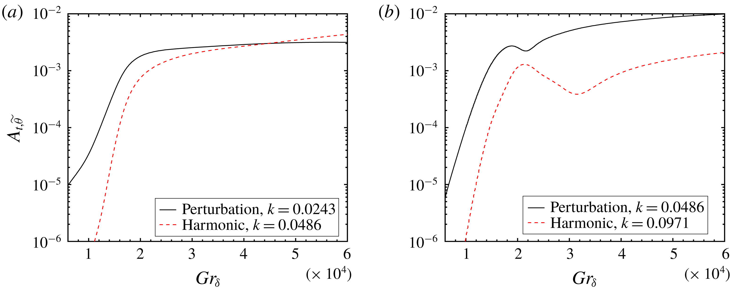
Development of the harmonics; (a) case DNS-A, initial perturbation
 $k=0.0243$
; (b) case DNS-B, initial perturbation
 $k=0.0486$
; perturbations (black solid); harmonic waves (red dashed).

At some large
 $Gr_{\unicode[STIX]{x1D6FF}}$
the unstable temporal signals (cases DNS-A and DNS-B) no longer follow the exponential growth of the sinusoidal signals, indicating nonlinear behaviour as the boundary layer grows thicker. The development of the harmonics, which are usually generated by the nonlinear interactions, are compared with that of the initial perturbations to investigate this nonlinearity. As indicated by figure 9, the higher harmonics of the perturbation waves are both increasing their strength as the base flow continues to evolve. In figure 9(a), the harmonic mode (
 $k=0.0486$
) grows rapidly and later overwhelms the initial perturbation at large
 $Gr_{\unicode[STIX]{x1D6FF}}$
, as the harmonic mode at
 $k=0.0486$
is less stable to the base flow than the initial perturbation (
 $k=0.0243$
) according to the marginal stability plane (figure 2). The harmonic mode in this case not only receives energy from the initial perturbation but also gets amplified by the base flow. In figure 9(b), since the discrete mode at
 $k=0.0971$
experiences damping for
 $Gr_{\unicode[STIX]{x1D6FF}}>7000$
in the linear regime, the development of the harmonic mode (
 $k=0.0971$
) depends solely on the nonlinear mechanisms. Consequently, the resultant nonlinearity in the case DNS-A appears more powerful than in the case DNS-B (see also figure 8) as the harmonic wave is amplified much more quickly than the initial perturbation.
The temporal response of discrete wavenumber
 $k=0.0486$
is also examined using three-dimensional direct numerical simulations. To investigate the effect of the initial conditions, the laminar flow is initialized at
 $Gr_{\unicode[STIX]{x1D6FF}_{0}}=22.5$
for case DNS-D and at
 $Gr_{\unicode[STIX]{x1D6FF}_{0}}=3000$
for case DNS-E and case DNS-F. The amplitude of the finite disturbance is chosen as
 $A_{n}=10^{-3}$
for case DNS-D and case DNS-F and
 $A_{n}=10^{-2}$
for case DNS-E. In case DNS-F, multiple temperature normal modes, in the form of equation (5.1), are added to the base flow solution to thermally perturb the boundary layer
 $$\begin{eqnarray}\tilde{\unicode[STIX]{x1D703}}_{x}=\unicode[STIX]{x1D703}_{b}(y)A_{n}\mathop{\sum }_{r=0}^{7}\sin \left(2^{r}\frac{2\unicode[STIX]{x03C0}x}{L_{x}}\right),\end{eqnarray}$$
where
 $r$
is an integer specifying the components of the sinusoidal perturbation. While the base flow lies in the laminar linear regime, each of the individual components are expected to interact linearly with the base flow.
Random background white noise, given in equation (5.2), is also superposed on the initial temperature field to trigger the three-dimensional laminar–turbulent transition for three-dimensional simulations (Nakao et al. Reference Nakao, Hattori and Suto2017). It is written as
 $$\begin{eqnarray}\tilde{\unicode[STIX]{x1D703}}_{0}=A_{0}[\text{RAND}(0,1)-0.5],\end{eqnarray}$$
where
 $A_{0}$
is the amplitude of the background white noise and
 $\text{RAND}(0,1)$
denotes a random number generator which generates statistically uniformly distributed random numbers between
 $0$
and
 $1$
. Additional tests have been carried out, not shown here for brevity, to ensure that the amplification rate of the streamwise normal modes are not affected by the amplitude of the background noise
 $A_{0}$
, which is set to
 $10^{-6}$
for the results presented.
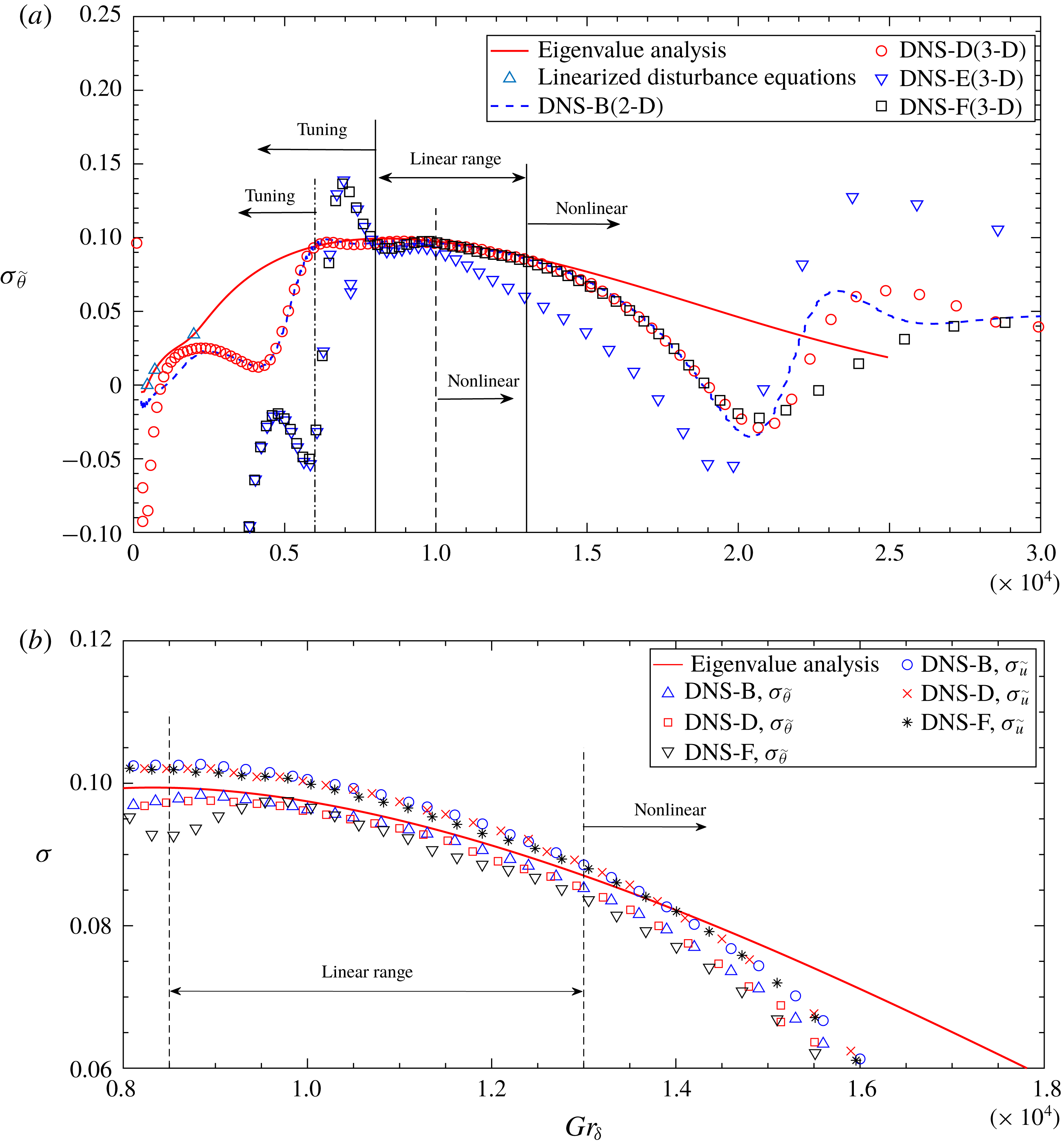
Amplification rate comparison for wavenumber
 $k=0.0486$
; (a) temperature amplification rate; (b) velocity and temperature amplification rate in the linear range of the unsteady flow (not all data are shown for clarity).

In figure 10, the amplification rate
 $\unicode[STIX]{x1D70E}_{k}$
of the perturbation mode
 $k=0.0486$
is compared with the linear stability results. Due to the inevitable receptivity, the perturbation does not follow the prediction of the linear stability analysis instantly but is tuned by the base flow to a suitable magnitude for a short period after it is introduced into the flow. Such receptivity effects can also be observed in DNS-B in figure 10(a) where both temperature and velocity fields are perturbed by the solutions to the linearized disturbance equations, indicating the magnitude and phase relation obtained from the ‘frozen base flow’ no longer holds for the unsteady base flow due to the additional terms in the unsteady Navier–Stokes equations. Consequently, we are not able to determine the minimum value of
 $\unicode[STIX]{x1D70F}_{0}$
, or equivalently
 $Gr_{\unicode[STIX]{x1D6FF}}$
, for which the quasi-steady approximation is valid, i.e. to what extent can
 $Gr_{\unicode[STIX]{x1D6FF}}$
be deemed as ‘large enough’ so that the slowly varying base flow assumption holds. At large
 $Gr_{\unicode[STIX]{x1D6FF}}$
, as depicted by figure 10, the amplification rate predicted by the quasi-steady eigenvalue analysis shows reasonably good agreement with the direct stability analysis in the linear range.
The two-dimensional simulation (case DNS-B) shows similar development to the three-dimensional simulations (cases DNS-D and DNS-F) up to the initial stage of the nonlinear behaviour (before the amplification rate reaches its minimum at around
 $Gr_{\unicode[STIX]{x1D6FF}}\sim 2\times 10^{4}$
for cases DNS-D and DNS-F). The velocity amplification rate (
 $\unicode[STIX]{x1D70E}_{\tilde{u} }$
) is found to be slightly larger than that of the temperature (
 $\unicode[STIX]{x1D70E}_{\tilde{\unicode[STIX]{x1D703}}}$
) in the linear region as shown in figure 10(b), so that equation (4.3) does not hold for the unsteady base flow. In contrast, Brooker et al. (Reference Brooker, Patterson, Graham and Schöpf2000) reported that the temperature signal is amplified more rapidly than the velocity signal for water (
 $Pr=7$
). This suggests that the ratio of
 $\unicode[STIX]{x1D70E}_{\tilde{\unicode[STIX]{x1D703}}}$
to
 $\unicode[STIX]{x1D70E}_{\tilde{u} }$
could be Prandtl number dependent.
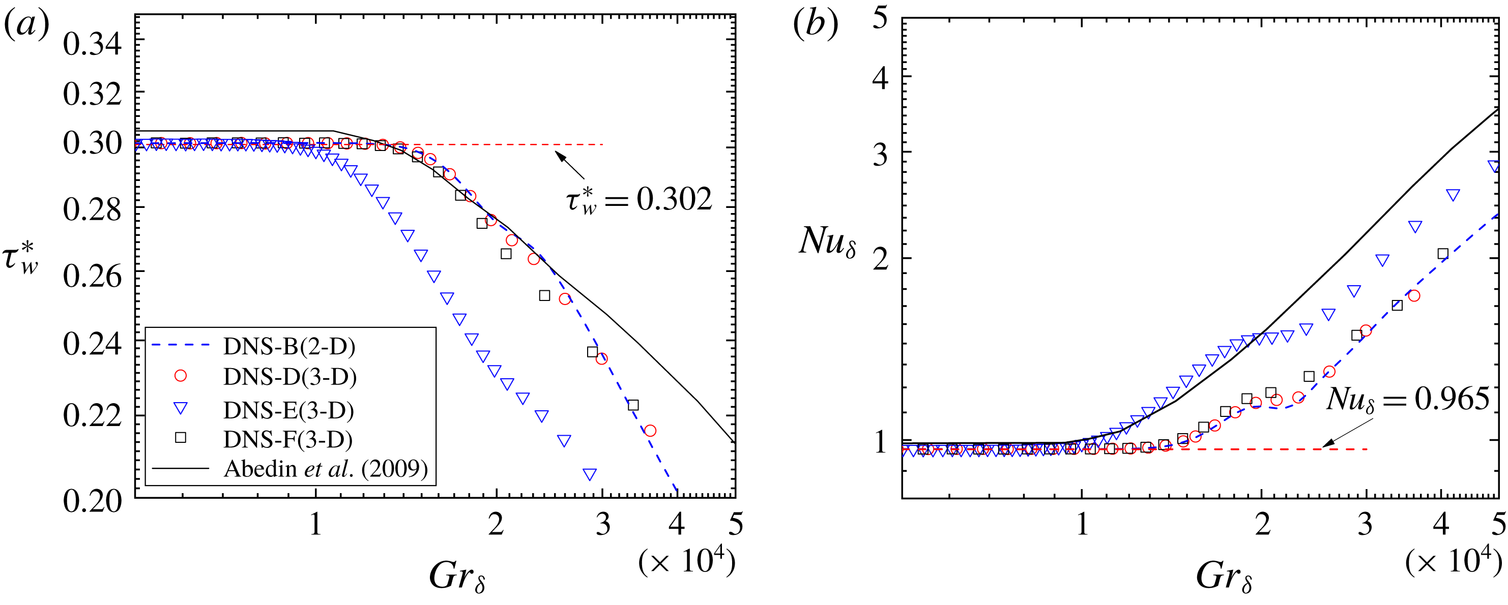
Mean flow statistics (not all data are shown for clarity), (a) normalized wall shear stress development; (b) the Nusselt number development.

In cases DNS-B, DNS-D and DNS-F, at about
 $Gr_{\unicode[STIX]{x1D6FF}}\sim 1.3\times 10^{4}$
the amplification rate obtained by direct stability analysis differs from the eigenvalue solution, indicating the onset of the nonlinearity. This Grashof number, on the other hand, coincides well with the sudden change in the mean flow statistics such as the wall shear stress and the Nusselt number, as shown in figure 11. Here, the wall shear stress
 $\unicode[STIX]{x1D70F}_{w}=\unicode[STIX]{x1D708}\unicode[STIX]{x2202}u/\unicode[STIX]{x2202}y$
is normalized by
 $$\begin{eqnarray}{\unicode[STIX]{x1D70F}_{w}}^{\ast }=\unicode[STIX]{x1D70F}_{w}/(\unicode[STIX]{x1D70C}g\unicode[STIX]{x1D6FD}\unicode[STIX]{x1D703}_{w}\unicode[STIX]{x1D6FF})\end{eqnarray}$$
and the Nusselt number is defined by
 $$\begin{eqnarray}Nu_{\unicode[STIX]{x1D6FF}}=-\frac{\unicode[STIX]{x1D6FF}\displaystyle \left.\frac{\unicode[STIX]{x2202}\unicode[STIX]{x1D703}}{\unicode[STIX]{x2202}y}\right|_{y=0}}{\unicode[STIX]{x1D703}_{w}}.\end{eqnarray}$$
Since the mean flow velocity and temperature distribution follow the analytical solution (2.3), an analytical correlation of the normalized wall shear stress and the Nusselt number can be derived in equation (5.5)
 $$\begin{eqnarray}\displaystyle & \displaystyle Nu_{\unicode[STIX]{x1D6FF}}=\frac{\unicode[STIX]{x1D6FF}}{\sqrt{\unicode[STIX]{x03C0}t}}\sim 0.965, & \displaystyle\end{eqnarray}$$
 $$\begin{eqnarray}\displaystyle & \displaystyle \unicode[STIX]{x1D70F}_{w}^{\ast }=\frac{2\sqrt{Prt}}{\sqrt{\unicode[STIX]{x03C0}}\unicode[STIX]{x1D6FF}(\sqrt{Pr}+1)}\sim 0.302. & \displaystyle\end{eqnarray}$$
 $Gr_{\unicode[STIX]{x1D6FF}}\sim 10^{4}$
. This point is the critical Grashof number that indicates the onset of laminar–turbulent transition of the unsteady NCBL. Such sudden changes in the mean flow statistics were also observed in a DNS study for the temporally developing NCBL by Abedin et al. (Reference Abedin, Tsuji and Hattori2009) (shown in figure 11), where they also noted a transition point of approximately
 $Gr_{\unicode[STIX]{x1D6FF}}\sim 10^{4}$
. Nevertheless it can be seen in figure 11 that the transition point from Abedin et al. (Reference Abedin, Tsuji and Hattori2009) occurs at a slightly larger
 $Gr_{\unicode[STIX]{x1D6FF}}$
than our DNS-E. It is worth noting that Abedin et al. (Reference Abedin, Tsuji and Hattori2009) used an ensemble average of the transition value
 $Gr_{\unicode[STIX]{x1D6FF}}$
with different initial disturbances to obtain their result. The difference in the perturbation modes, method and amplitude may contribute to the discrepancy to the present study. Nakao et al. (Reference Nakao, Hattori and Suto2017) also indicated that the grid resolution may have an impact on such transition behaviour in large eddy simulations. However, the present direct numerical simulations fully resolve all length and time scales in the flow, and the solver tolerance is very tight, to the extent that if no discrete perturbation is applied the flow remains one-dimensional and no perturbation appears in the solution.
From figures 10 and 11, it can be seen that the choice of the initialization of the laminar flow in terms of
 $Gr_{\unicode[STIX]{x1D6FF}_{0}}$
(at which time instant the perturbations are fed into the laminar base flow) has minimal effect on the transition Grashof number. However, the initial amplitude of the infinitesimal perturbation plays an important role in determining this parameter. A ten-fold increase in the initial perturbation amplitude leads to an earlier transition without having much effect in the tuning and linear range.
6 Conclusion
In this paper, the stability properties of an unsteady, temporally evolving NCBL adjacent to an isothermally heated vertical wall are investigated, first as an eigenvalue problem with a ‘frozen’ base flow. The eigenvalue results show that the base flow is initially filtering for a specific marginally unstable wavenumber, and broadening to a range of unstable wavenumbers with increasing
 $Gr_{\unicode[STIX]{x1D6FF}}$
. At high enough
 $Gr_{\unicode[STIX]{x1D6FF}}$
in the linear region, the initially unstable modes are damped. Consequently, in contrast to the observations in the spatially developing NCBL flows (Dring & Gebhart Reference Dring and Gebhart1968, Reference Dring and Gebhart1969), the most amplified frequency is not necessarily higher than the initially unstable wavenumber (
 $k=0.0544$
), but strongly depends on the pathway through the marginal stability map.
The critical
 $Gr_{\unicode[STIX]{x1D6FF}}$
at which a single mode first becomes unstable is found to be
 $Gr_{\unicode[STIX]{x1D6FF}}=454.2$
, with the most unstable wavenumber
 $k=0.0544$
. At the critical point, the phase velocity
 $U_{p}$
of the most unstable wavenumber is found to be the same as the maximum velocity
 $U_{m}$
of the base flow, which was also observed by Armfield & Patterson (Reference Armfield and Patterson1992). However, the corresponding critical
 $Gr_{\unicode[STIX]{x1D6FF}}$
for a spatially developing NCBL is found at a much higher value (Nachtsheim Reference Nachtsheim1963) due to differences in the shape of the base flow profile.
Both two- and three-dimensional direct numerical simulations have been performed at different initial conditions to further investigate the instability of the unsteady flow. We found that unlike the ‘frozen’ base flow cases, where the amplification rates of both velocity
 $\unicode[STIX]{x1D70E}_{\tilde{u} }$
and temperature
 $\unicode[STIX]{x1D70E}_{\tilde{\unicode[STIX]{x1D703}}}$
are identical, the velocity signals are amplified at a slightly higher rate than the temperature signals when the unsteadiness and nonlinear effects are incorporated, and the ratio
 $\unicode[STIX]{x1D70E}_{\tilde{u} }/\unicode[STIX]{x1D70E}_{\tilde{\unicode[STIX]{x1D703}}}$
may depend on the Prandtl number
 $Pr$
.
The amplification rates predicted by the eigenvalue analysis and direct numerical simulations are similar in the linear range (see figure 11) up to a transition point, showing that the instantaneous stability properties of an unsteady, temporally evolving NCBL are very similar to those of a steady NCBL at the same local
 $Gr_{\unicode[STIX]{x1D6FF}}$
. However, the perturbation taken from the linearized ‘frozen’ base flow still undergoes the receptivity process (see case DNS-B), indicating the magnitude and phase relation of the perturbation obtained in the steady, linearized NCBL does not hold in the unsteady NCBL.
The Grashof number at laminar–turbulent transition, where a sudden change in mean flow statistics occurs is related to the initial amplitude of the perturbation, but is found to be independent of the time (in terms of
 $Gr_{\unicode[STIX]{x1D6FF}}$
) that the perturbations are applied (provided they are small enough). From the present study, the transition value is
 $Gr_{\unicode[STIX]{x1D6FF}}\sim 1\times 10^{4}$
for
 $A_{n}=10^{-2}$
and
 $Gr_{\unicode[STIX]{x1D6FF}}\sim 1.3\times 10^{4}$
for
 $A_{n}=10^{-3}$
. It is evident that the laminar–turbulent transition is closely related to the onset of the nonlinearity of the flow.