I. INTRODUCTION
Thin films are widely used in various applications to enhance the surface properties and characteristics of materials. They are used in biomedical, automotive, aeronautic, military, electronic, and energy domains. Reference Lopes, Vieira, Borges, Fernandes, Rodrigues, Alves, Barradas, Apreutesei, Steyer, Tavares, Cunha and Vaz1–Reference Tait, Worfolk, Maloney, Hauger, Elias, Buriak and Harris3 The physical properties of coatings often differ from those of bulk materials and depend essentially on the techniques of elaboration and their parameters. Reference Billard and Perry4,Reference Thornton5 So to optimize the reliability and the performance of coated components, the physical, chemical, and mechanical properties of a coating must be controlled. In this paper the interest will be focused on the elastic modulus of thin films.
In the last two decades, many methods were developed to determine the elasticity constants of bulk and coated materials which can be classified into two groups: static and dynamic techniques. Reference Bellan and Dhers6,Reference Radovic, Lara-Curzio and Riester7 Among the dynamic techniques, we can mention in particular the resonant ultrasound spectroscopy Reference Tan, Shyam, Choi, Lara-Curzio and Sampath8–Reference Thomasová, Sedlák, Seiner, Janovská, Kabla, Shilo and Landa10 and the vibrational technique. Reference Bellan and Dhers6,Reference Gadaud and Pautrot11–Reference Mazot and Pautrot14 In the following, more attention will be given to the determination of the coatings Young’s modulus using the vibrational approach also known as the Impulse Excitation Technique (IET).
All the mathematical relations are based on the Euler–Bernoulli bending beam theory which does not take into account the effect of shear and rotatory inertia. To consider both effects, Pickett has simplified the Timoshenko’s equation and determined some correction factors. Reference Pickett15 Then these factors were improved by Spinner and Tefft Reference Tefft16–Reference Tefft and Spinner19 who have determined the correcting factors as a function of different vibration modes and sample geometry. Their works have led to the birth of the ASTM-E1876 test method in 1999, updated in 2015. 20
The IET is a nondestructive technique, highly precise and easy to use to measure the elasticity constants of a wide range of materials: metals, composites, ceramics, coatings … etc. Reference Radovic, Lara-Curzio and Riester7,Reference Gadaud and Pautrot11,Reference Gadaud, Milhet and Pautrot13,Reference Atri, Ravichandran and Jha21 These advantages qualify this technique to be adopted as another alternative to measure the Young’s modulus of coatings. The first experience using a bilayer material (substrate + coating) was carried out by Berry. Reference Berry and Pritchet22 The test relies on the measurement of the sample resonance frequencies before and after deposition.
Many researchers have used the IET for various films elaborated differently with different thickness. By comparing four measurement methods, Bellan et al. Reference Bellan and Dhers6 have shown that IET gives good and accurate results. They have evaluated the elasticity modulus of SiC and PyC films elaborated by Chemical Vapor Deposition (CVD) with 35 µm and 95 µm of thickness, respectively. López-Puerto, Reference López-Puerto and Oliva12 Peraud, Reference Peraud, Pautrot, Villechaise, Mazot and Mendez23 and Etienne Reference Etienne, Ayadi, Nivoit and Montagnon24 have measured the Young’s modulus of various thin films, respectively: Au/Al, SiC/NiTi (2 µm obtained by dynamic ion mixing) and TiN (0.2 µm elaborated by ion implantation). All these authors have used different mathematical relations. The lack of information concerning the validity range of the models and the observed divergence between them, in the case of higher ratio of coating/substrate thickness, gives the motivation to do a thorough study on the models proposed in the literature. Also, a thorough study of error/uncertainty sources seems to be inexistent in the literature.
The goal of this paper is not only to review all the mathematical relations developed to determine the Young’s modulus of coatings but also to investigate their advantages, limits and do an investigation on the measurement accuracy. Although the method applied here is very general, the quantitative description is based on experiments performed on aluminum films, as a concrete example. Firstly, we introduce the theoretical background of the IET and review the models. Secondly, we present the deposition conditions of the aluminum film and the followed experimental protocol to determine its Young’s modulus. Then, we compare all the analytical expressions with the finite element model and studying the impact of the assumptions on the validity of each model. Finally, an uncertainty study is realized to identify the errors or uncertainty sources and evaluate their contributions.
II. MEASUREMENT PRINCIPLES
A. Theoretical background
Based on the Euler–Bernoulli beam theory which does not take into account the shear and rotary inertia effect, the motion of a beam subjected to flexural vibration can be described by the following equation Reference Rao25 :
 $$\rho S{{{\partial ^2}U\left( {x,t} \right)} \over {\partial {t^2}}} + {{{\partial ^2}} \over {\partial {x^2}}}\left( {EI{{{\partial ^2}U\left( {x,t} \right)} \over {\partial {x^2}}}} \right) = 0\quad .$$
This differential equation can be solved analytically and allows to determine the shapes and the frequencies of the vibration modes. The resonance frequencies can be determined from this following equation Reference Rao25 :
 $${f_n} = {{X_n^2} \over {{l^2}}}\sqrt {{{EI} \over {\rho S}}}$$
Where:X n : constant which depends on the boundary conditions applying to the beam (called also nondimensional eigenfrequencies).
In the present study, we used a free–free system for which:
 $${X_n} = \left( {2n + 1} \right){\pi \over 2}\quad.$$
B. Homogeneous beam
The IET is not only used for beam specimen but can be used for any sample shape: rod, disc, and arbitrary geometry. 20,Reference Pagnotta and Stigliano26 In the case of a free–free beam with a rectangular cross-section, the Young’s modulus can be determined by the following formula [Eq. (4)] 20 :
 $$E = {k_1}f_{\rm{s}}^2{\rho _{\rm{s}}}{{{l^4}} \over {h_{\rm{s}}^2}}{T_{\rm{f}}}\quad.$$
Where:
 $${k_1}\,\sim\,0.9465\quad.$$
Index s means the substrate.
T f is the geometrical correction factor introduced to take into account the shear and rotatory effects. 20
 $${T_{\rm{f}}} = 1 + 6.585\left( {1 + 0.0752v + 0.8109{v^2}} \right){\left( {{{{h_{\rm{s}}}} \over l}} \right)^2} - 0.868{\left( {{{{h_{\rm{s}}}} \over l}} \right)^4} - \left[ {{{8.34\left( {1 + 0.2023v + 2.173{v^2}} \right){{\left( {{{{h_{\rm{s}}}} \over l}} \right)}^4}} \over {1 + 6.338\left( {1 + 0.1408v + 1.536{v^2}} \right){{\left( {{{{h_{\rm{s}}}} \over l}} \right)}^2}}}} \right]$$
If
 $l/{h_{\rm{s}}} \;\ge\; 20$
, it can be simplified into the following expression:
 $${T_{\rm{f}}} = 1 + {k_2}{\left( {{{{h_{\rm{s}}}} \mathord{\left/ {\vphantom {{{h_{\rm{s}}}} l}} \right. \kern-\nulldelimiterspace} l}} \right)^2}$$
Where:
 $${k_2}\,\sim\,6.585\quad.$$
C. Extension to coated substrates
The principle of the measurement is to perform a two-steps frequency measurement before and after deposition. Then knowing the elastic modulus of the substrate, the density of both substrate and coating and the resonance frequencies of the composite beam and the substrate, the Young’s modulus of the film can be determined through analytical expressions. In the literature, all models, allowing to determine the coating Young’s modulus, are based on two different theories: the flexural rigidity of a composite beam and the classical laminated beam theory.
III. REVIEW OF THE MODELS PROPOSED IN THE LITERATURE
A. Models based on the flexural rigidity of a composite beam
During bending, a composite beam is loaded with a moment. The resistance to this moment (EI), also known as the flexural rigidity, of the entire composite beam can be expressed as the sum of the flexural rigidity of each material [Eq. (7)]. Reference Gere27 The coating is supposed to be perfectly homogeneous, compact, and adherent to the substrate.
 $${E_{\rm{t}}}{I_{\rm{t}}} = {E_{\rm{s}}}{I_{\rm{s}}} + {E_{\rm{c}}}{I_{\rm{c}}}$$
The indexes t, s, and c mean whole (homogenized) bilayer beam, substrate, and coating, respectively.
The density per unit of area of the composite beam can be determined by the following equation:
 $${\rho _{\rm{t}}}{S_{\rm{t}}} = {\rho _{\rm{s}}}{S_{\rm{s}}} + {\rho _{\rm{c}}}{S_{\rm{c}}}\quad .$$
By replacing EI by E t I t and ρS by the effective density of the composite beam ρt S t in Eq. (2) we will obtain the resonance frequency of the composite beam:
 $${f_{\rm{t}}} = {{X_n^2} \over {{l^2}}}\sqrt {{{{E_{\rm{t}}}{I_{\rm{t}}}} \over {{\rho _{\rm{t}}}{S_{\rm{t}}}}}}\quad.$$
1. Lopez’s model
For a composite beam with a rectangular cross section, Lopez has developed an analytical expression to determine the film Young’s modulus. The second moments of substrate and coating sections are respectively calculated as follows:
 $${I_{\rm{s}}} = {{bh_{\rm{s}}^3} \over {12}}\quad,$$
 $${I_{\rm{c}}} = {{b{h_{\rm{c}}}h_{\rm{s}}^2} \over 4} + {{b{h_{\rm{s}}}h_{\rm{c}}^2} \over 2} + {{bh_{\rm{c}}^3} \over 3}\quad.$$
Replacing I s and I c by their correspondent expressions, in Eq. (9), leads to the frequencies ratio between the coated sample and the substrate. Reference Mazot and Pautrot14,Reference François28
 $${\left( {{R_{\rm{f}}}} \right)^2} = {{1 + {R_{\rm{E}}}\left( {3{R_{\rm{h}}} + 6R_{\rm{h}}^2 + 4R_{\rm{h}}^3} \right)} \over {1 + {R_{\rm{h}}}{R_\rho }}}$$
Where:
 $${R_{\rm{h}}} = {{{h_{\rm{c}}}} \over {{h_{\rm{s}}}}}$$
 $${R_\rho } = {{{\rho _{\rm{c}}}} \over {{\rho _{\rm{s}}}}}$$
 $${R_{\rm{f}}} = {{{f_{\rm{t}}}} \over {{f_{\rm{s}}}}}$$
 $${R_{\rm{E}}} = {{{E_{\rm{c}}}} \over {{E_{\rm{s}}}}}\quad.$$
Then, the Young’s modulus of the coating can be calculated as:
 $${E_{\rm{c}}} = {{{E_{\rm{s}}}} \over {3{R_{\rm{h}}} + 6R_{\rm{h}}^2 + 4R_{\rm{h}}^3}}\left[ {\left[ {{{\left( {{R_{\rm{f}}}} \right)}^2}\left( {1 + {R_{\rm{h}}}{R_\rho }} \right)} \right] - 1} \right]\quad .$$
This model does not consider the shift of the neutral axis after deposition. This simplification becomes increasingly inaccurate when the film thickness increases and for large R E ratio.
2. Pautrot’s model
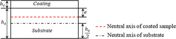
The difference between Lopez’s model and Pautrot’s model is that the latter takes into account the shift of the neutral axis after deposition (Fig. 1). This shift can be determined by the equation which establishes the equilibrium of forces. Reference Gere27
 $$\int_{ - {h_{\rm{s}}} + e}^e {{\sigma _{\rm{s}}}\,{\rm{d}}S} + \int_e^{e + {h_{\rm{c}}}} {{\sigma _{\rm{c}}}\,{\rm{d}}S} = 0$$
 $$e = {{{E_{\rm{s}}}h_{\rm{s}}^2 - {E_{\rm{c}}}h_{\rm{c}}^2} \over {2{E_{\rm{s}}}{h_{\rm{s}}} + 2{E_{\rm{c}}}{h_{\rm{c}}}}}$$
 $${I_{\rm{s}}} = {{bh_{\rm{s}}^3} \over {12}} + b{h_{\rm{s}}}{\left( {{{{h_{\rm{s}}}} \over 2} - e} \right)^2}$$
 $${I_{\rm{c}}} = {{bh_{\rm{c}}^3} \over {12}} + b{h_{\rm{c}}}{\left( {e + {{{h_{\rm{c}}}} \over 2}} \right)^2}$$
Schematic representation of the shift of the neutral axis after deposition.

Taking into consideration the shift of the neutral axis (e) in the expressions of second moments of both substrate and coating and replacing them in Eq. (9) lead to obtain the frequencies ratio between the coated sample and the substrate. Reference Gadaud and Pautrot11,Reference Mazot and Pautrot14,Reference François28
 $${\left( {{R_{\rm{f}}}} \right)^2} = {{1 + R_{\rm{h}}^3{R_{\rm{E}}} + {{3{R_{\rm{h}}}{R_{\rm{E}}}{{\left( {1 \;+\; {R_{\rm{h}}}} \right)}^2}} \over {1 \;+\; {R_{\rm{h}}}{R_{\rm{E}}}}}} \over {1 + {R_{\rm{h}}}{R_{\rm{E}}}}}$$
Inverting Eq. (18) leads to getting the following second degree equation which allows to determine the Young’s modulus of the coating.
 $$A{\left( {{R_{\rm{E}}}} \right)^2} + B\left( {{R_{\rm{E}}}} \right) + C = 0$$
Where
 $$A = {\left( {{R_{\rm{h}}}} \right)^4}$$
 $$B = 4{\left( {{R_{\rm{h}}}} \right)^3} + \left( {6 - {R_\rho }R_{\rm{f}}^2} \right){\left( {{R_{\rm{h}}}} \right)^2} + \left( {4 - R_{\rm{f}}^2} \right)\left( {{R_{\rm{h}}}} \right)$$
 $$C = 1 - R_{\rm{f}}^2\left( {1 + {R_\rho }{R_{\rm{h}}}} \right)$$
Based on the same hypothesis of the flexural rigidity, this bilayer model has been extended analytically to a three layers model. Reference Mazot and Pautrot14 It has been used to determine the Young modulus of the interface layer (E i) between the coating and the substrate. Reference Mazot and Pautrot14
 $${\left( {{R_{\rm{f}}}} \right)^2} = {{1 + 4{R_{{{\rm{h}}_{\rm{i}}}}}{R_{{{\rm{E}}_{\rm{i}}}}} + 4{R_{\rm{h}}}{R_{\rm{E}}}} \over {1 + {R_{{{\rm{h}}_{\rm{i}}}}}\left( {{R_{{{\rm{E}}_{\rm{i}}}}} + {R_{{\rho _{\rm{i}}}}}} \right) + {R_{\rm{h}}}\left( {{R_{\rm{E}}} + {R_\rho }} \right)}}$$
The indexes i and t mean the interface and the three layers beam respectively.Where:
 $${R_{{{\rm{h}}_{\rm{i}}}}} = {{{h_{\rm{i}}}} \over {{h_{\rm{s}}}}}$$
 $${R_{{{\rm{E}}_{\rm{i}}}}} = {{{E_{\rm{i}}}} \over {{E_{\rm{s}}}}}$$
 $${R_{{\rho _{\rm{i}}}}} = {{{\rho _{\rm{i}}}} \over {{\rho _{\rm{s}}}}}$$
 $${R_{\rm{f}}} = {{{f_{\rm{t}}}} \over {{f_{\rm{s}}}}}\quad.$$
3. Berry’s model
Berry’s model Reference Berry and Pritchet22 is a simplified approach which can be obtained from the first order Taylor series expansion of either Pautrot’s or Lopez’s models.
 $${\left( {{R_{\rm{f}}}} \right)^2} = 1 + {R_{\rm{h}}}\left[ {3{R_{\rm{E}}} - {R_\rho }} \right]$$
 $${E_{\rm{c}}} = {{{E_{\rm{s}}}} \over 3}\left[ {{R_\rho } + {{{{\left( {{R_{\rm{f}}}} \right)}^2} - 1} \over {{R_{\rm{h}}}}}} \right]$$
B. Model based on the classical laminated beam theory (CLBT)
This model is based on the classical laminated beam theory, and allows the determination of the elasticity modulus of an individual thin film in multilayers coatings. Reference López-Puerto and Oliva12 It uses the assumption that the laminated beam is symmetric, which does not correspond to the common configuration where a film is deposited only on one side of the substrate. However, the formalism can be used as an approximation for asymmetric configuration but it becomes inaccurate in the case of thick films and large R E and R ρ ratios. In the case of a free–free beam, the frequency of multilayers coatings can be expressed as:
 $${f_{\rm{t}}} = {{3.561} \over {{l^2}}}\sqrt {{1 \over {{d_{11}}{\rho _{{\rm{eff}}}}}}}\quad.$$
The frequency ratio:
 $${\left( {{R_{\rm{f}}}} \right)^2} = 11.37{{{\rho _{\rm{s}}}} \over {{d_{11}}{\rho _{{\rm{eff}}}}{E_{\rm{s}}}}}\quad.$$
For a one layer coating (substrate + coating):
 $${d_{11}} = {{{{{H_1}{E_{\rm{s}}}} \over {3\left( {1 - \nu _{\rm{s}}^2} \right)}} + {{{H_2}{E_{\rm{c}}}} \over {3\left( {1 - \nu _{\rm{c}}^2} \right)}}} \over {{{\left[ {{{{H_1}{E_{\rm{s}}}} \over {3\left( {1 - \nu _{\rm{s}}^2} \right)}} + {{{H_2}{E_{\rm{c}}}} \over {3\left( {1 - \nu _{\rm{c}}^2} \right)}}} \right]}^2} + {{\left[ {{{{H_1}{\nu _{\rm{s}}}{E_{\rm{s}}}} \over {3\left( {1 - \nu _{\rm{s}}^2} \right)}} + {{{H_2}{\nu _{\rm{c}}}{E_{\rm{c}}}} \over {3\left( {1 - \nu _{\rm{c}}^2} \right)}}} \right]}^2}}}$$
 $$\left\{ {\matrix{ {{H_1} = {{{{\left( {{h_{\rm{s}}} \;+\; {h_{\rm{c}}}} \right)}^3}} \over 4} - {{3{{\left( {{h_{\rm{s}}} \;+\; {h_{\rm{c}}}} \right)}^2}{h_{\rm{c}}}} \over 4} \;+\; {{3\left( {{h_{\rm{s}}} \;+\; {h_{\rm{c}}}} \right)h_{\rm{c}}^2} \over 2} - h_{\rm{c}}^3} \cr {{H_2} = {{3{{\left( {{h_{\rm{s}}} \;+\; {h_{\rm{c}}}} \right)}^2}{h_{\rm{c}}}} \over 4} - {{3\left( {{h_{\rm{s}}} \;+\; {h_{\rm{c}}}} \right)h_{\rm{c}}^2} \over 2} + h_{\rm{c}}^3} \cr} } \right.$$
 $${\rho _{{\rm{eff}}}} = {\rho _{\rm{s}}}{h_{\rm{s}}} + {\rho _{\rm{c}}}{h_{\rm{c}}}\quad.$$
In this section we have illustrated the developed models to determine the coating Young’s modulus using the vibrational method. Peraud Reference Peraud, Pautrot, Villechaise, Mazot and Mendez23 and Etienne Reference Etienne, Ayadi, Nivoit and Montagnon24 have respectively used Berry’s and Pautrot’s models to determine the Young’s modulus of deposited films. Mazot Reference Mazot and Pautrot14 noted that the Berry’s model and Lopez’s model starts to diverge for a thickness ratio of coating to substrate in the order of 0.1. The difference between the models becomes larger for higher ratios. To analyze quantitatively the differences between the models, a comparison with a finite element model, taken as a reference will be performed to assess the trueness of the method. Then, an uncertainty analysis will be done to compare the behavior of the different models with regard to their sensitivity to various uncertainty sources.
IV. EXPERIMENTS
A. Deposition
Aluminum film was deposited on a stainless steel 316L substrate by DC magnetron sputtering using a 99.99% purity aluminum target, 200 mm in diameter. The chamber was pumped down with a turbomolecular pump to less than 10−7 Pa before filling it with argon. The target-to-substrate distance was kept equal to 11 cm and the substrate holder was rotating to ensure a perfect thickness homogeneity of the coating. The intensity applied to the aluminum target thanks to a pulsed-DC Advanced Energy Pinnacle power supply was 2.5 A (frequency = 50 kHz; time off = 5 µs) and the argon flow rate of 20 sccm led to a chamber pressure of 0.2 Pa. The substrate dimensions are its length l = 70.5 mm, its width b = 15.68 mm, and its thickness h s = 0.98 mm. The coating has the same length and width as the substrate and a thickness h c = 6.712 μm.
B. Measurement of dimensions and density
The dimensions of the substrate were measured ten times in ten different locations. The mass of the substrate was measured using a Sartorius precision balance and its density was evaluated: ρs = 7738 kg/m3.
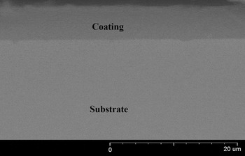
After deposition, the mass of the bilayer sample was measured. By using a scanning electron microscope, the thickness of the film was measured ten times in different positions. Figure 2 presenting a fractured cross sectional SEM image shows that there is no significant variation in the film thickness. The difference in mass measured before and after deposition corresponds to the film. Considering the mass and the dimensions of the film, its density was estimated: ρc = 2655 kg/m3.
Cross sectional SEM image of the aluminum film.

C. IET experimental set-up
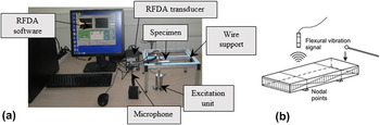
The principle of the IET is to measure the resonance frequencies of a specimen impacted by an impulse (Fig. 3). A beam can be excited in different vibrational modes: longitudinal, flexural, and torsional. 20 These mechanical vibrations are detected by an acoustic microphone, and transformed by a transducer into an electrical signal which is presented as a function of time. Finally, the Fast Fourier Transform (FFT) is used to represent the signal as a function of frequency and extract the resonance frequencies of the sample. The resonance frequency, density or mass and dimensions of the sample are used to calculate the elastic constants of the material.
(a) Experimental equipment, (b) flexural vibration mode. Reference Atri, Ravichandran and Jha21

Before performing the test, the specimen is placed on a support (Fig. 3). The free–free boundary condition was adopted for the present procedure. 20 To achieve as best as possible this free–free condition, several supporting methods were used:
-
(i) foam strips presenting a very low stiffness but for which the contact is large
-
(ii) wires located at the nodal points of the sample where the displacement is equal to zero (for the first flexural mode used in the present study).
More detailed explanations on the procedure can be found in the literature. 20,Reference Lord and Morrell29 During the test some errors on the measured frequency can be introduced throughout any of the used equipment or the misplacement of the sample. These sources of error will be investigated below.
The measurement of frequencies was done with the RFDA professional signal analysis system (Resonance Frequency and Damping Analysis) from IMCE company (Genk, Belgium). It is equipped with an RFDA transducer, an automatic excitation unit, a microphone with a frequency range up to 100 kHz, a universal wire support and a computer system equipped with RFDA software (Fig. 3).
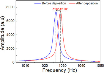
The first resonance frequency was measured before and after deposition (Fig. 4). The two measured frequencies were used to calculate the substrate Young’s modulus using Eq. (4) and the film Young’s modulus with the different models using Eqs. (13), (19), (25), and (27). The values of the frequencies and Young’s modulus are represented in Table I.
Natural frequencies before and after deposition.

Substrate and film Young’s modulus.

V. NUMERICAL SIMULATION
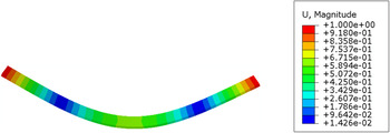
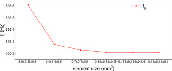
A 3D Finite Elements Model (FEM) was developed with the commercial finite element code ABAQUS 30 (Fig. 5). Figure 5 represent the first vibration mode of the bilayer beam. The geometrical model is composed of two parts: the substrate and the coating. The substrate is a rectangular cross section slender beam with a length l = 70 mm, a width b = 7 mm and a thickness h s = 0.5 mm. The coating was bonded on the substrate throughout the tie function 30 and has a thickness h c, which was varied during analysis from 0 to 0.25 mm. Free boundary conditions were applied to the beam and the 3D stress C3D20 quadratic element was used to mesh the structure. To extract the resonance frequency of the composite beam, the ABAQUS\Implicit Lanczos eigensolver was used. A mesh convergence study was done (Fig. 6), and the element size of (0.35 × 0.35 × 0.25 mm3) was chosen. This configuration is chosen as a reference to compare the analytical models proposed in the literature.
Deformed beam. The colors indicate the vertical displacement (mm).

Mesh convergence.

VI. TRUENESS ANALYSIS
In the metrological field, trueness is defined as the agreement of the measured value (averaged on an infinite number of measurements) and a reference value, as defined, for instance by a standard. 31 It is associated with the notion of systematic error. In the case of the Young’s modulus of thin film, the traceability to international standards is not established and no certified reference material is available. Thus it is difficult to perform a trueness study satisfactorily. However, in the present paper, two sources of systematic errors are investigated: the error linked to the model, with the FEM of Sec. V as an arbitrary reference and the error linked to the effective realization of the free–free boundary condition (which is done in Sec. VII. A. 4).
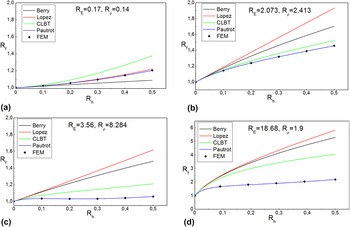
In this section a parametric comparison of the analytical models with the finite element model is done for four different R E and R ρ ratios. Figure 7 represents the evolution of the frequency ratio R f as a function of the thickness, density, and Young’s modulus ratios. We can see a very good agreement between Pautrot’s model and the FEM, for any R h, R E, and R ρ ratios. This good agreement means that, at least in the range explored in the present study, the rotatory and the shear effects are sufficiently corrected by the T f factor of Eq. (6) in the analytical model. It is interesting to note that, in Figs. 7(c) and 7(d), the frequency variation versus R h tends to stabilize which means that, for these configurations, the obtained modulus is not very sensitive to the film thickness.
Comparison between analytical and numerical models for different Young’s modulus and density ratios: (a) R E = 0.17, R ρ = 0.14, (b) R E = 2.073, R ρ = 2.413, (c) R E = 3.56, R ρ = 8.284, (d) R E = 18.68, R ρ = 1.9.

The divergence of the other models can be clearly seen. This divergence is due to the different assumptions on which is based each model. It can be seen that the difference between the models increases with R h ratio which was expected from the assumptions made in each model. It can be observed that the differences between the models and the reference value do not always appear in the same order. For small values of R E and R ρ, Lopez model is the closest to the Pautrot/MEF solution while, for other configurations, it is CLBT which is the closest.
A. Models systematic error study
In this work, we evaluate the systematic error of the different models taking as a reference the finite element model developed in Sec. V. As mentioned in Sec. V, there is no guarantee that the FE model presents the true value.
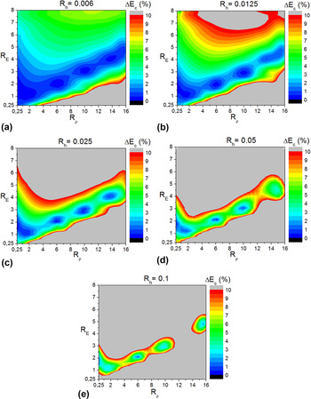
To estimate the errors, extensive series of numerical analyses were carried out by the commercial finite element ABAQUS. The thickness ratio R h was varied from 0.006 to 0.1, the Young’s modulus ratio R E from 0.25 to 8 and the density ratio from 0.25 to 16. The results are presented in Figs. 8–10.
Systematic error associated to Lopez’s model.

Systematic error associated to Berry’s model for different Young’s modulus, density and thickness ratios: (a) R h = 0.006, (b) R h = 0.0125, (c) R h = 0.025, (d) R h = 0.05, (e) R h = 0.1.

Systematic error associated to CLBT’s model.

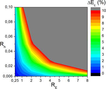
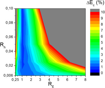
Figure 8 shows the evolution of the systematic error of Lopez’s model as a function of Young’s modulus ratio R
E and thickness ratio R
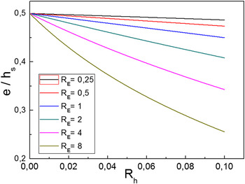
h. The gray zone represents an error higher than 10%. It is clearly seen that the evolution of the error is proportional to the evolution of the distance e between the neutral axis before and after deposition (Figs. 1 and 11). Figure 11 represent the evolution of the normalized shift of the neutral axis
 ${e \over {{h_{\rm{s}}}}}$
as a function of the ratios R
E and R
h. The lower error zone, between 1 and 2%, is limited by a Young’s modulus ratio equal to 1 and a thickness ratio equal to 0.02. On the other side, we found that the error of the Lopez’s model does not depend on the density ratio R
ρ (even though R
ρ appears in the expression of Lopez’s model) so that we can conclude that the trueness error of the Lopez’s model is related to the thickness and Young’s modulus ratios.
Evolution of the normalized shift of the neutral axis e/h s as a function of the thickness and Young’s modulus ratios.

Contrarily to Lopez’s model, the error of Berry’s model (Fig. 9) depends on the density ratio R ρ, the Young’s modulus ratio R E, and the thickness ratio R h. Figure 9 represents the evolution of the error as a function of the thickness, Young’s modulus and density ratios. We can see that for higher thickness ratio the error is more important for the same Young’s modulus and density ratios. It is interesting to note that there is a correlation between R E and R ρ on the systematic error and thus that an increase of one of the two ratio will not systematically lead to an increase of the error. For instance, for a small error will be obtained for R ρ = 14 and R E = 4. Using Berry’s model, it is necessary to keep attention to the ratios mentioned above. Figure 9 can provide information about the error made.
Like Lopez’s model, the error of the CLBT model does not depend on the density ratio R ρ. On Fig. 10 we can see the evolution of the CLBT model error as a function of the thickness and the Young’s modulus ratios. We can observe that the optimum error zone is centered at a Young’s modulus ratio equal to 1. This is due to the assumption of symmetry on which is based this model.
VII. UNCERTAINTY ANALYSIS
The uncertainty analysis is performed following the guidelines of current reference metrological document, i.e., the Guide to the Expression of Uncertainty in Measurement (aka GUM), ISO 57 020 standard 32 and the International Vocabulary of Metrology (aka VIM), JCGM 200:2012. 31 The uncertainty on a quantity x is denoted u(x) which represents the standard uncertainty, that is, the standard deviation of the distribution of x values, obtained either experimentally from a series of measurements either estimated from various assumptions. Not all the uncertainty sources are taken into account in the present paper. For instance the definitional uncertainty and the instrumental measurement uncertainty were neglected. The former represents the uncertainty linked to the definition of the measurand while the latter denotes the uncertainty arising from the measurement system. Here, the measurand (the measured quantity) is defined as the Young’s modulus of the unique specimen, i.e., fluctuations due to the manufacturing process are neglected and its value is assumed to be homogeneous in the film or in the substrate. The elastic behavior of the film and the substrate is assumed to follow the isotropic Hooke’s law, i.e., the effects of texture, for instance, are neglected. Uncertainties coming from the measurement system such as those linked to the window used for computing the FFT and the signal discretization are assumed to be negligible. It can be noted that the GUM methodology can be criticized by some experts in metrology, however its aim is to be standardized to be relatively easy to use by a non-expert in metrology.
Some components of the uncertainty considered in the present study can be calculated using the uncertainty propagation equation, like in the study done by Bullough, Reference Bullough33 and some others do not appear explicitly in the models. The latter are generally linked to the measurement technique and the apparatus. In our case the frequency is investigated (repeatability and sample positioning) and its uncertainty calculated experimentally.
A. Frequency error investigations
An experimental study was done to estimate the uncertainty on the measured frequency through the different possible sources of error. In the following we will present the sources which influence significantly the frequency measurement.
1. Repeatability
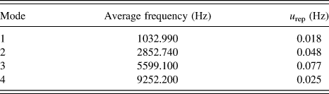
The RFDA system (Fig. 3) was used to determine the first four flexural resonance frequencies of a slender steel substrate which dimensions are given in Sec. IV. A. The nylon wires support provided with the instrument was taken as a reference. To excite the desired mode, the wires of the supports were located at the respective nodal points of each mode. Each measurement was repeated thirty times, and then repeated again on a different days in the same conditions and by the same operator. The microphone was placed at a distance of 5 mm from the substrate. The angle between the nodal lines of the beam and the wires of the support is 0°. The average frequency and the repeatability uncertainty are presented in Table II. The repeatability uncertainty is calculated using Eq. (31), according to the GUM. 32
 $${u_{{\rm{rep}}}} = {{{\sigma _{\exp }}} \over {\sqrt j }}$$
Where j is the number of repeated frequency measurements and σexp is the standard deviation computed on the j measurements.
Repeatability uncertainty of the first four resonance frequencies.

2. Position of the microphone
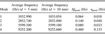
To study the influence of the microphone position on the frequency measurement, the microphone was placed at a distance of 5 and 10 mm from the sample. The angle between the nodal lines and the support wires was kept at 0°. The resonances frequencies measured in both configurations are presented in Table III. The difference Δf posit is higher than the repeatability uncertainty, so the effect of the microphone position can be considered as significant (Tables II and III). Assuming that the error caused by the position of the microphone on the frequency follows a uniform distribution function between the two values obtained, the standard uncertainty can be calculated using Eq. (32) 32 :
 $${u_{{\rm{posit}}}} = {{\Delta {f_{{\rm{posit}}}}} \over {2\sqrt 3 }}\quad.$$
Effect of microphone position on the measured resonance frequencies.

3. Misalignment between the nodal lines and the supporting wires
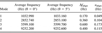
To study the influence of the misalignment between the nodal lines and the supporting wires on the frequency measurement, the specimen was placed on the universal support forming an angle of 5° and the microphone was placed at 5 mm from the specimen. The measured frequencies were compared with the values of Table II which correspond to 0°. The comparison is presented in Table IV. The quantity Δf align is higher than the repeatability uncertainty, so the effect of misalignment is considered as significant. Like in the previous section, assuming that the error caused by the misalignment between the nodal lines and the supporting wires on the frequency follows a uniform distribution function between the two measured values, the standard uncertainty is calculated using Eq. (33) 32
 $${u_{{\rm{align}}}} = {{\Delta {f_{{\rm{align}}}}} \over {2\sqrt 3 }}\quad.$$
Misalignement’s error.

In fact, a misalignment of 5° is easy to spot and, in practice, the corresponding uncertainty will certainly be smaller. Here, the misalignment was exaggerated to make it detectable.
4. Supports
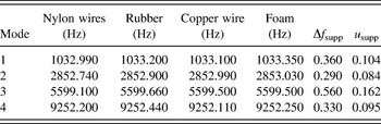
In the models, the boundary conditions for the beam are assumed to be free–free. However, this condition is not possible in practice and different solutions can be imagined to get as close as possible to the modeling assumptions. To evaluate the influence of the nature of the support, the first four frequencies were measured by using the following supports: Nylon wire, rubber, copper wire and foam. The results are illustrated in Table V. The highest difference between the measured frequencies is higher than the repeatability uncertainty. The effect of support is thus considered as significant and the quantity Δf supp is used to calculate the uncertainty u supp caused by the support.
 $${u_{{\rm{supp}}}} = {{\Delta {f_{{\rm{supp}}}}} \over {2\sqrt 3 }}$$
Resonance frequencies of the sample placed on different supports.

B. Uncertainty of the substrate and the film Young’s moduli
Firstly we will explicit all the uncertainties which appear in Eq. (4), then the global combined standard uncertainty of the substrate Young’s modulus will be calculated according to the equation of uncertainty propagation given in the GUM, assuming that the covariances between the different quantities are null 32 :
 $$u{\left( {{E_{\rm{s}}}} \right)^2} = {\left( {{{\partial {E_{\rm{s}}}} \over {\partial {k_1}}}} \right)^2}u{\left( {{k_1}} \right)^2} + {\left( {{{\partial {E_{\rm{s}}}} \over {\partial {k_2}}}} \right)^2}u{\left( {{k_2}} \right)^2} + {\left( {{{\partial {E_{\rm{s}}}} \over {\partial {f_{\rm{s}}}}}} \right)^2}u{\left( {{f_{\rm{s}}}} \right)^2} + {\left( {{{\partial {E_{\rm{s}}}} \over {\partial {\rho _{\rm{s}}}}}} \right)^2}u{\left( {{\rho _{\rm{s}}}} \right)^2} + {\left( {{{\partial {E_{\rm{s}}}} \over {\partial l}}} \right)^2}u{\left( l \right)^2} + {\left( {{{\partial {E_{\rm{s}}}} \over {\partial {h_{\rm{s}}}}}} \right)^2}u{\left( {{h_{\rm{s}}}} \right)^2}\quad.$$
1. Frequency uncertainty
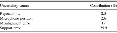
The uncertainty of the first resonance frequency can be calculated by adding the square of the standard uncertainty (adding the variances) of each quantity on the measurement. In the previous section, it has been shown that the uncertainty due to the support is the most influent on the measurement.
 $$u\left( {{f_{\rm{s}}}} \right) = \sqrt {u_{{\rm{rep}}}^2 + u_{{\rm{posit}}}^2 + u_{{\rm{align}}}^2 + u_{{\rm{supp}}}^2} = 0.115\;{\rm{Hz}}$$
Table VI shows the contribution of each uncertainty source on the uncertainty of frequency. We can see clearly that the support has the highest contribution to the global uncertainty, then the uncertainty due to the misalignment. The influence of the two other sources is small (about 5%).
Contribution of each source error on the uncertainty of frequency.

2. k 1 and k 2 constants uncertainty
Supposing that the constants k 1 and k 2 were rounded, we can consider that the true value of k 1 is between 0.94645 and 0.94655 and the true value of k 2 is between 6.5845 and 6.5855. The constants uncertainty is then calculated as follows:
 $$u\left( {{k_1}} \right) = {{0.0001} \over {2\sqrt 3 }} = {2.810^{ - 5}}$$
 $$u\left( {{k_2}} \right) = {{0.001} \over {2\sqrt 3 }} = {2.810^{ - 4}}\quad.$$
It should be noted that these uncertainties are not physical but they are due to the finite number of digits available. The uncertainty budget shows that the influence of rounding is negligible as compared to other uncertainty sources.
3. Dimensions uncertainties
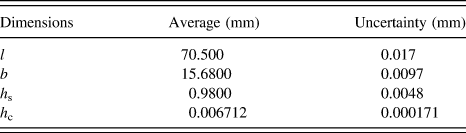
The dimensions of the substrate and the coating were measured ten times in ten different locations. The dimensions averages and their uncertainties are presented in Table VII. The standard uncertainties were evaluated according to a type A method by computing the standard deviation. 32
Dimensions of the substrate and measurement uncertainty.

4. Density uncertainty
The uncertainties on substrate and film densities are calculated using the sample mass and dimensions. The mass uncertainty is evaluated following a type B procedure.
32
According to the technical specifications of the precision balance used, the uncertainty is equal to 1 mg so the standard deviation was taken equal to
 $1/\sqrt 3 \;{\rm{mg}}$
. The uncertainties on the substrate and the film densities are calculated as follow
32
:
 $$u{\left( {{\rho _{\rm{s}}}} \right)^2} = {\left( {{{\partial {\rho _{\rm{s}}}} \over {\partial {m_{\rm{s}}}}}} \right)^2}u{\left( {{m_{\rm{s}}}} \right)^2} + {\left( {{{\partial {\rho _{\rm{s}}}} \over {\partial {h_{\rm{s}}}}}} \right)^2}u{\left( {{h_{\rm{s}}}} \right)^2} + {\left( {{{\partial {\rho _{\rm{s}}}} \over {\partial l}}} \right)^2}u{(l)^2} + {\left( {{{\partial {\rho _{\rm{s}}}} \over {\partial b}}} \right)^2}u{(b)^2}$$
 $$u\left( {{\rho _{\rm{s}}}} \right) = 39\;{{{\rm{kg}}} \mathord{\left/ {\vphantom {{{\rm{kg}}} {{{\rm{m}}^{\rm{3}}}}}} \right. \kern-\nulldelimiterspace} {{{\rm{m}}^{\rm{3}}}}}$$
 $$u{\left( {{\rho _{\rm{c}}}} \right)^2} = {\left( {{{\partial {\rho _{\rm{c}}}} \over {\partial {m_{\rm{c}}}}}} \right)^2}u{\left( {{m_{\rm{c}}}} \right)^2} + {\left( {{{\partial {\rho _{\rm{c}}}} \over {\partial {h_{\rm{c}}}}}} \right)^2}u{\left( {{h_{\rm{c}}}} \right)^2} + {\left( {{{\partial {\rho _{\rm{c}}}} \over {\partial l}}} \right)^2}u{(l)^2} + {\left( {{{\partial {\rho _{\rm{c}}}} \over {\partial b}}} \right)^2}u{(b)^2}\quad.$$
 $$u\left( {{\rho _{\rm{c}}}} \right) = 149\;{{{\rm{kg}}} \mathord{\left/ {\vphantom {{{\rm{kg}}} {{{\rm{m}}^{\rm{3}}}}}} \right. \kern-\nulldelimiterspace} {{{\rm{m}}^{\rm{3}}}}}$$
5. Global uncertainty
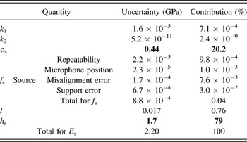
From all the uncertainties calculated in previous sections, the global uncertainty on the substrate Young’s modulus was calculated using Eq. (35). The substrate Young’s modulus uncertainty and the contribution of each uncertainty source are presented in Table VIII. A contribution correspond to one of the terms in Eq. (35).
Contribution of each uncertainty source on the substrate Young’s modulus uncertainty.

From Table VIII, we can conclude that the main contribution to the global uncertainty comes from the measurement of the thickness (79%) and of the density (20%). The other quantities are completely negligible. So, to increase the accuracy of Young’s modulus measurement, the main efforts should be put on the accuracy of thickness.
After calculating of the uncertainty on the elasticity modulus of the substrate (Table VIII), the uncertainty of the coating Young’s modulus is calculated according to the GUM, the uncertainty was calculated for all the models (Berry, Pautrot, Lopez and CLBT) to see the difference between the generated uncertainty of each model because it may happened that a more accurate model can be less stable and lead to a larger uncertainty than a simplified model, but in this case the frequency uncertainty is treated differently. The support error is now considered as systematic given that the same support will be used to measure the two frequencies before and after deposition, causing a similar shift of the two frequencies. So, to evaluate the error due to the support, it will be integrated in the different models (Pautrot, Berry, Lopez and CLBT) through the frequency ratio R f.
 $${R_{\rm{f}}} = {{{f_{\rm{t}}} + {\Delta _{{\rm{supp}}}}} \over {{f_{\rm{s}}} + {\Delta _{{\rm{supp}}}}}}$$
Here, the error due to the support is assumed to be additive. If the error is assumed to be multiplicative, it will simplify out and lead to no error at all. Then, inverting Eqs. (13), (19), (25) and (27), the Young modulus of the film can be expressed as following:
 $${E_{\rm{c}}} = {E_{\rm{s}}}F\left( {{f_{\rm{t}}},{f_{\rm{s}}},{h_{\rm{c}}},{h_{\rm{s}}},{\rho _{\rm{c}}},{\rho _{\rm{s}}},{\Delta _{{\rm{supp}}}}} \right)\quad.$$
Where F is a function which depends on the model used. As Δsupp is smaller than 1 Hz and thus small as compared to f s or f t, function F can be expanded into a Taylor series and truncated to the first order. It was found that the support error represents a systematic error of about 5 × 10⁻³%. Based on this value, in the present case, the support error will be neglected in the calculation of uncertainty on the coating Young’s modulus, but will be kept in the uncertainty on the substrate Young’s modulus. This approach simplifies significantly the calculation of the uncertainty. Indeed, if the propagation of uncertainty was performed directly on Eq. (42) without the simplification, some correlations (covariances) would appear and become delicate to treat.
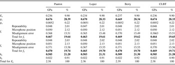
The uncertainty values and the contribution of each uncertainty source on the uncertainty of the coating Young’s modulus are represented in Table IX.
Contribution of each uncertainty source (in GPa and %) on the coating Young’s modulus uncertainty.

In our case the uncertainty is in the order of 2.4 GPa (Table IX) which represents 3.5% of the measured Young’s modulus. From Table IX, we can conclude that for all the models, the measure of the density and the thickness of the film, representing respectively a percentage contribution about 28% and 21% are the first to be improved. Contrarily to the case of the substrate, the uncertainty on the frequency has a significant effect on the measurement and increases from 0.04% to 19%. This is related to the small difference between the frequencies measured before and after deposition. More attention on the alignment of the nodal points of the sample with the support can give a higher precision on the measured value. It can be noted that no difference was observed on the uncertainty of the different models, nor on the magnitude of the different sources. This means that it is always better to use the more complete model. This is not always the case in inverse methods.
VIII. CONCLUSION
The Young’s modulus of coatings and substrates was measured by the Impulse Excitation Technique (IET). The elasticity modulus of the coating was obtained by different models available in the literature: Berry, Lopez, Pautrot and Classical Laminated Beam Theory. A numerical finite element model was developed and used to estimate the systematic errors given by the four analytical models. A detailed uncertainty budget was performed for each model according to the recommendation of the ISO Guide on the Expression of Uncertainty on Measurement. The following results were obtained:
-
(1) The reliability of Berry’s model depends on the thickness, density and Young’s modulus ratios and not only on the thickness ratio.
-
(2) Both Lopez and CLBT models depend on the thickness and Young’s modulus ratios. Increasing these ratios increases the error.
-
(3) Pautrot’s model is the most complete and it presents an almost perfect agreement with the numerical values obtained by finite elements. It is thus recommended to determine the Young’s modulus of a film for any thickness, Young’s modulus and density ratios.
-
(4) The standard uncertainty on the substrate Young’s modulus is about 2.2 GPa and it is about 2.4 for the coating which, in the case of the studied material, represents about 3.5% of the measured value.
-
(5) The standard uncertainty on the substrate Young’s modulus comes mainly from the uncertainty on its density and on its thickness. For the coating itself, the main sources of uncertainty are the density and the thickness of the coating and the frequency before and after coating. The 4 models used to calculate the Young’s modulus give the same total uncertainty and the same weight of all the sources.
NOMENCLATURE

ACKNOWLEDGMENTS
The authors would like to thank Région Champagne-Ardenne and Accompagnement Economique du Laboratoire de Bure-Saudron for the financial support.