1 Introduction
Liquid metal batteries (LMBs) are discussed today as one option for economic grid-scale energy storage that is indispensable for the further development of fluctuating renewable electricity sources. The design of LMBs is very simple. They consist of three stably stratified liquid layers housed in a closed container. A light alkaline metal floats on the top, a heavy metal or half-metal alloy is placed at the bottom and a thin layer of a molten-salt electrolyte is sandwiched in between. The electrolyte is chosen to be conductive to ions of the light metal.
The liquid–liquid salt–metal interfaces facilitate extremely fast charge transfer and high current densities, making the LMB in combination with low ohmic losses an efficient and flexible stationary energy storage device (Kim et al. Reference Kim, Boysen, Newhouse, Spatocco, Chung, Burke, Bradwell, Jiang, Tomaszowska, Wang, Wei, Ortiz, Barriga, Poizeau and Sadoway2013). Further, LMBs offer high potential of being low cost due to the simple fabrication and easy scalability at the cell level. And not least, a high cycle life is enabled by the liquid nature of the battery that naturally prevents structure degradation.
However, the easy scalability to large-size cells together with the very high current densities (up to
 $13~\text{A}~\text{cm}^{-2}$
, Cairns & Shimotake Reference Cairns and Shimotake1969a
) can result in large currents. For this reason, large-size cells are potentially susceptible to magnetohydrodynamical (MHD) instabilities. They may have positive effects on the one hand, e.g. fluid motion in the metal layers can improve the mixing of reactants. On the other hand, strong metal flows can severely deform the interfaces such that the salt layer may be disrupted causing a short-circuit. Hence, it is of crucial importance to study the impacts of flow instabilities on the batteries to enable a secure operation in future large cells.
Several instability mechanisms have been identified in the last decade that can arise in LMBs. Primarily, the Tayler instability (TI) has been intensively studied (Stefani et al. Reference Stefani, Weier, Gundrum and Gerbeth2011; Weber et al. Reference Weber, Galindo, Stefani, Weier and Wondrak2013, Reference Weber, Galindo, Stefani and Weier2015b ; Herreman et al. Reference Herreman, Nore, Cappanera and Guermond2015) and it was found that the TI can be reliably controlled e.g. by applying axial magnetic fields, central counter currents or modifying the cell geometry. Further, electro-vortex flows (Weber et al. Reference Weber, Galindo, Priede, Stefani and Weier2015a ; Stefani et al. Reference Stefani, Galindo, Kasprzyk, Landgraf, Seilmayer, Starace, Weber and Weier2016) as well as thermal and Marangoni convection due to Joule heating in the electrolyte (Kelley & Sadoway Reference Kelley and Sadoway2014; Shen & Zikanov Reference Shen and Zikanov2016; Köllner, Boeck & Schumacher Reference Köllner, Boeck and Schumacher2017) have been investigated. However, in recent years long-wave interfacial instabilities, in particular the so-called metal pad roll instability (MPRI), emerged as the possibly most critical mechanism regarding the operation safety of shallow batteries (Bojarevics & Tucs Reference Bojarevics, Tucs and Ratvik2017; Weber et al. Reference Weber, Beckstein, Herreman, Horstmann, Nore, Stefani and Weier2017b ; Zikanov Reference Zikanov2017). An overview of MHD instabilities investigated in LMBs is given by Weier et al. (Reference Weier, Bund, El-Mofid, Horstmann, Lalau, Landgraf, Nimtz, Starace, Stefani and Weber2017).
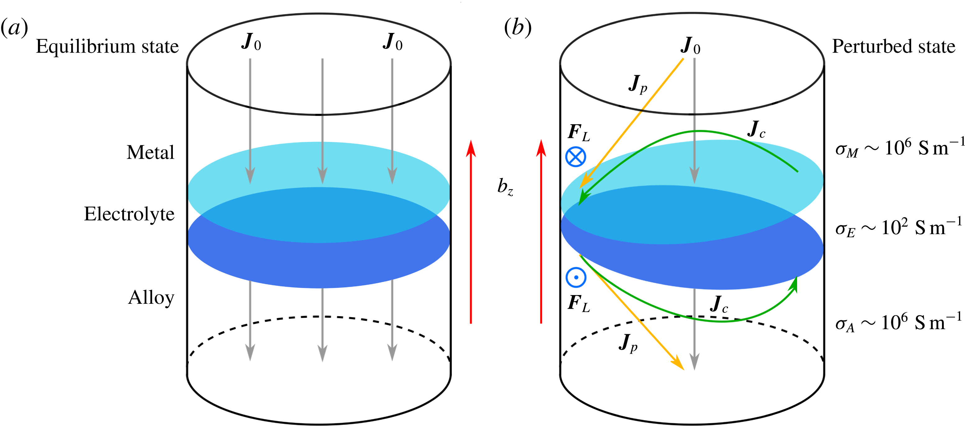
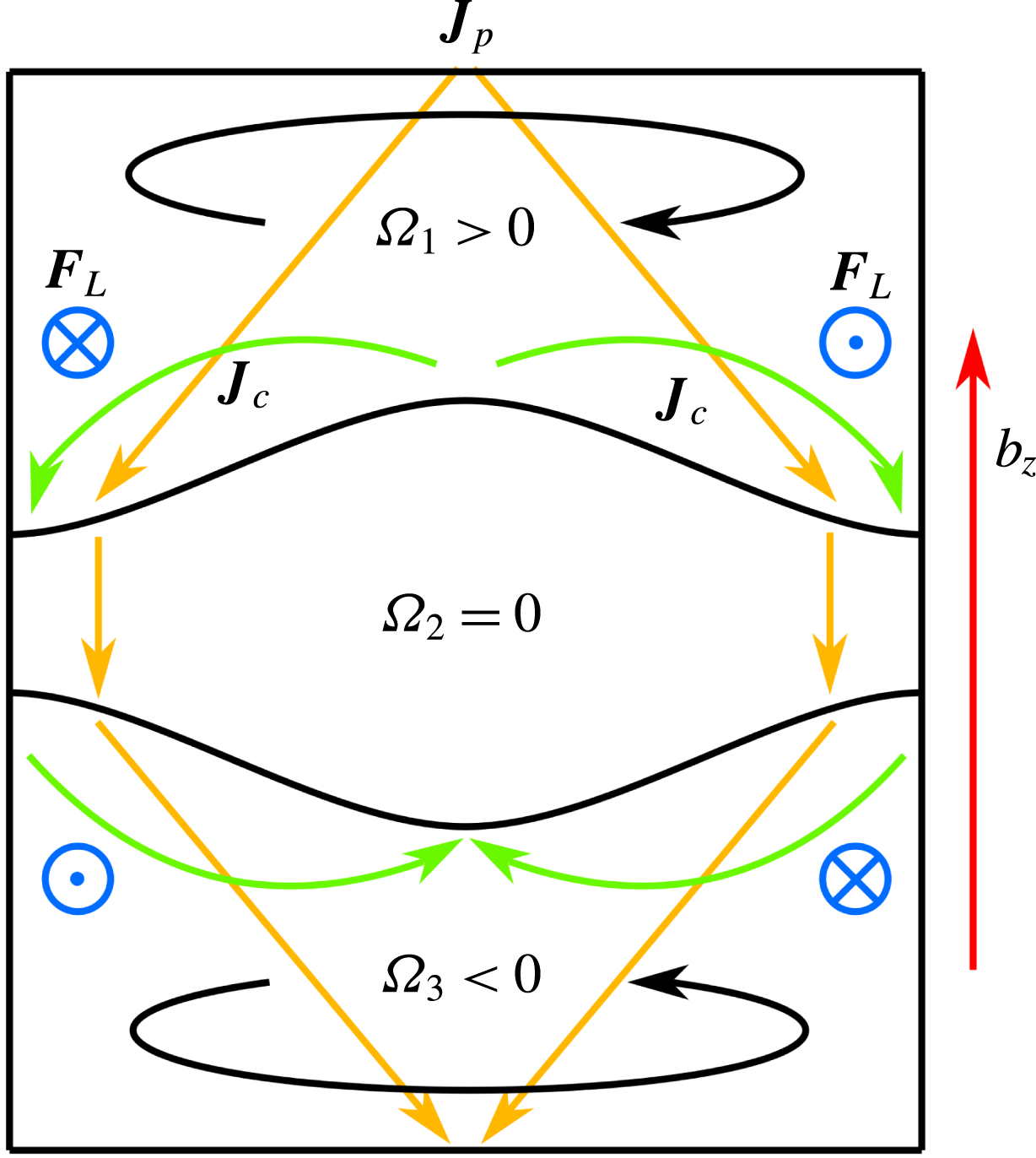
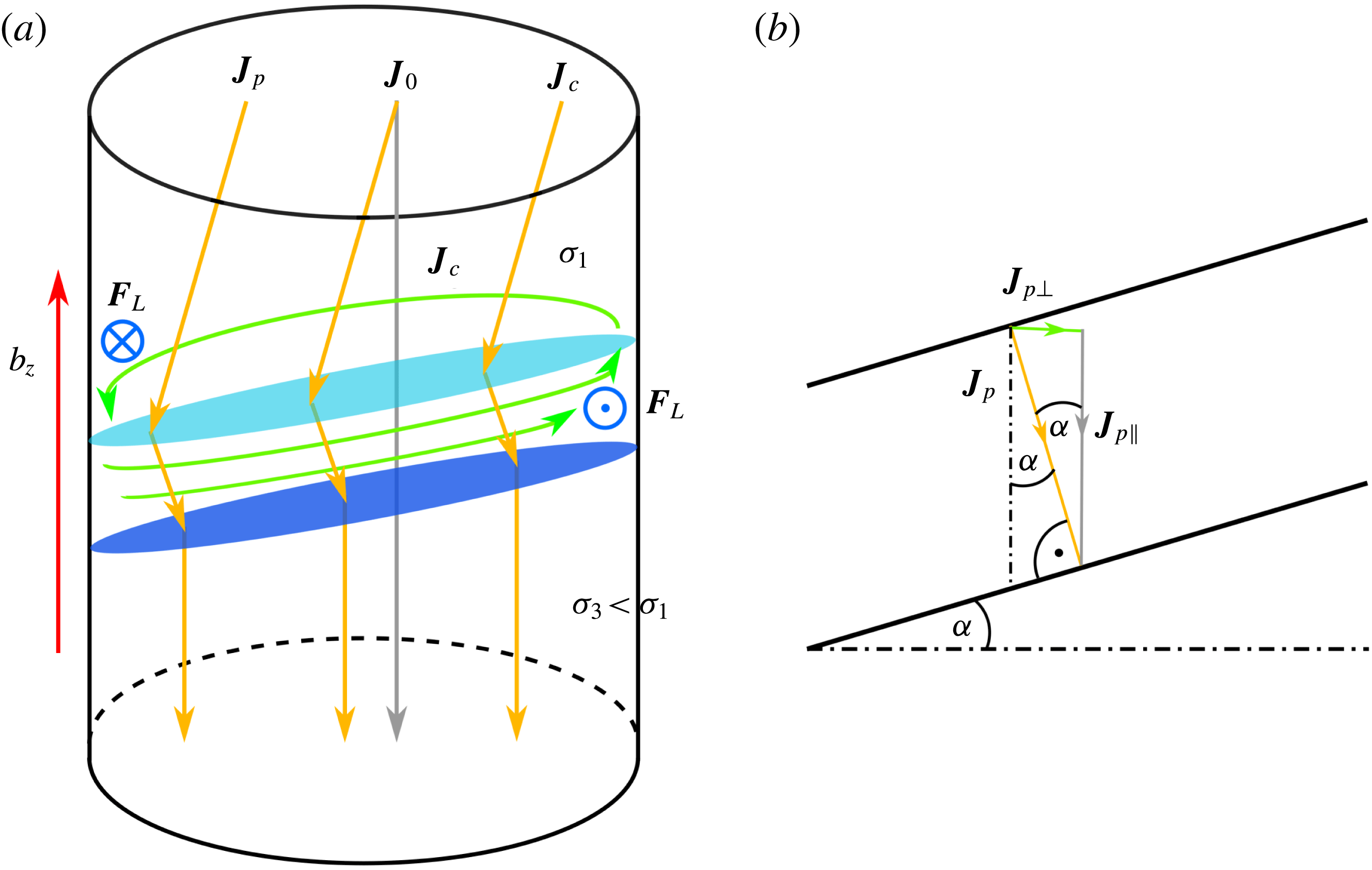
In the paper at hand, we aim to give a deeper understanding how the MPRI is manifested in LMBs incorporating hydrodynamically coupled interfaces. Originally, the MPRI was discovered in Hall–Héroult aluminium reduction cells (ARCs) that are related to LMBs. ARCs consist of two liquid layers, molten aluminium at the bottom and a cryolite bath with dissolved alumina floating on the top. The alumina is electrochemically reduced by applying strong cell currents. Sele (Reference Sele1977) was the first to give a qualitative explanation of the MPRI for two-layer reduction cells. Figure 1 illustrates his fundamental ideas expanded to three-layer LMBs: the key mechanism driving the metal pad is traced back to the interaction of horizontal currents with the vertical component of an external magnetic field
 $\boldsymbol{B}$
that can be induced, e.g. by supply lines. For simplicity, let us assume that the cell current density
 $\boldsymbol{J}_{0}$
is purely vertical during the charging or discharging and the magnetic field also purely vertical and homogeneous
 $\boldsymbol{B}=b_{z}\boldsymbol{e}_{z}$
. For fluid layers at rest,
 $\boldsymbol{J}_{0}$
and
 $b_{z}$
are parallel such that no motion is expected to arise in this idealized configuration (left cell). However, once one or both interfaces are slightly tilted (right cell), the current will be deflected. That is due to the orders of magnitude lower electrical conductivity of the electrolyte
 $\unicode[STIX]{x1D70E}_{E}$
in comparison to that of the electrode metals. The current must always take the path of least resistance i.e. where the electrolyte layer is thin. As a result, a redistributed non-vertical perturbation current
 $\boldsymbol{J}_{p}$
arises.
 $\boldsymbol{J}_{p}$
can be decomposed into the unperturbed vertical current
 $\boldsymbol{J}_{0}$
and a horizontal component that is denoted as the compensation current
 $\boldsymbol{J}_{c}$
. Together with
 $b_{z}$
the latter horizontal currents lead to horizontal Lorentz forces
 $\boldsymbol{F}_{L}$
here pointing inwards at the upper light metal and outwards at the heavy one. Finally, these Lorentz forces, which are perpendicular to the interfacial slope, drive the metals leading to rotational interfacial wave motion that is called the metal pad roll. Though, in contrast to the ARCs, from this picture it is not clear in which direction both interfaces will rotate since the induced Lorentz forces are oppositely directed. We will examine this topic in § 3.2.1. While the scenario sketched above provides a first intuitive feeling about the origin of the MPRI, the physical nature is actually far more complex. Stability analysis were performed in the last decades by Bojarevics & Romerio (Reference Bojarevics and Romerio1994), Sneyd & Wang (Reference Sneyd and Wang1994) and Davidson & Lindsay (Reference Davidson and Lindsay1998) showing that the Lorentz force can couple standing gravity waves leading to a rotation and exponential growth in the unstable limit. The instability mechanism can be described just as well by wave reflection at the tank walls (Lukyanov, El & Molokov Reference Lukyanov, El and Molokov2001).
Schematic explanation of the MPRI in LMBs. If both interfaces are at rest (left cell), the cell current density
 $\boldsymbol{J}_{0}$
is purely vertical for idealized boundary conditions and does not interact with likewise vertical external magnetic fields
 $b_{z}$
. Once one or both interfaces are somehow displaced, non-vertical perturbation currents
 $\boldsymbol{J}_{p}$
arise that are deflected to the wall where the low conducting electrolyte layer is thin.
 $\boldsymbol{J}_{p}$
comprises a horizontal component, the compensation current
 $\boldsymbol{J}_{c}$
, that induces horizontal Lorentz forces
 $\boldsymbol{F}_{L}$
in interaction with
 $b_{z}$
, finally driving a rotational wave motion.

Nevertheless, far less is known about the MPRI in LMBs yet. Zikanov (Reference Zikanov2015) first investigated long-wave coupling and stability using a simplified mechanical analogy inspired by Davidson (Reference Davidson2001). Very recently, the MPRI was numerically found in LMB models and identified as potentially dangerous using two-dimensional (2-D) shallow water (Bojarevics & Tucs Reference Bojarevics, Tucs and Ratvik2017; Zikanov Reference Zikanov2017) and 3-D direct numerical simulations (Weber et al.
Reference Weber, Beckstein, Herreman, Horstmann, Nore, Stefani and Weier2017b
). Bojarevics & Tucs (Reference Bojarevics, Tucs and Ratvik2017) and Weber et al. (Reference Weber, Beckstein, Herreman, Horstmann, Nore, Stefani and Weier2017b
) examined magnesium-antimony (
 $\text{Mg}\Vert \text{Sb}$
) batteries, where essentially only the upper interface was found to be excited. For this particular case LMBs act very similarly to ARCs. Weber et al. (Reference Weber, Beckstein, Herreman, Horstmann, Nore, Stefani and Weier2017b
) found that the stability can be roughly predicted by one dimensionless parameter
 $\unicode[STIX]{x1D6FD}$
, originally proposed by Sele (Reference Sele1977) for ARCs, reading
 $$\begin{eqnarray}\unicode[STIX]{x1D6FD}={\displaystyle \frac{I_{0}b_{z}}{h_{E}h_{M}(\unicode[STIX]{x1D70C}_{E}-\unicode[STIX]{x1D70C}_{M})g}},\end{eqnarray}$$
with
 $I_{0}$
denoting the total cell current,
 $h_{E}$
and
 $h_{M}$
the initial heights of the electrolyte and light metal layers,
 $\unicode[STIX]{x1D70C}_{E}$
and
 $\unicode[STIX]{x1D70C}_{M}$
the densities of the electrolyte and the light metal and
 $g$
the standard acceleration due to gravity.
 $\unicode[STIX]{x1D6FD}$
can be considered as the ratio of the magnetic force arising due to some interface displacement to the gravity force exerted on the interface for the same displacement. The metal pad roll is predicted to arise if
 $\unicode[STIX]{x1D6FD}$
exceeds some critical value
 $\unicode[STIX]{x1D6FD}_{c}$
that generally depends on the viscosity, interfacial tension and the cell geometry. Equation (1.1) implies that for a constant current density
 $J_{0}$
cells with a larger cross-sectional area
 $A$
are more likely to become unstable (
 $I_{0}=J_{0}A$
).
However, this criterion is not necessarily sufficient for LMBs. From (1.1) it is clear, that small density differences
 $\unicode[STIX]{x1D70C}_{E}-\unicode[STIX]{x1D70C}_{M}$
are destabilizing. In the investigated
 $\text{Mg}\Vert \text{Sb}$
cells, the density difference at the upper interface is much lower than the density difference at the lower one (
 $\unicode[STIX]{x1D70C}_{E}-\unicode[STIX]{x1D70C}_{M}\ll \unicode[STIX]{x1D70C}_{A}-\unicode[STIX]{x1D70C}_{E}$
) clarifying why only the upper interface is excited. Actually, this is not the case for most possible electrode metal combinations as we will show in § 2.4. In general, the two interfaces in LMBs can be closely coupled. That was very recently confirmed numerically by Zikanov (Reference Zikanov2017), who found strong interactions between the interfaces, when the electrolyte–metal density differences are comparable. However, the coupling mechanisms and dynamics are not yet understood, especially from the analytical point of view. Due to these facts, this paper investigates how the MPRI is manifested in universal LMBs with a variety of material combinations where both interfaces may be coupled and then be excited simultaneously.
In the first part, we present a theoretical potential flow analysis describing the hydrodynamical coupling of gravity–capillary waves bounded in cylindrical cells. Two independent dimensionless parameters are derived which completely determine the wave coupling. We demonstrate further that the interfaces can be coupled by two different coupling modes. In the second part, the theory is compared with direct numerical simulations (DNS). A parameter study is performed to investigate the impact of coupled interfaces on the stability. Three different coupling regimes are identified involving different characteristic coupling states and different stability properties. For strongly coupled LMBs we find novel types of instabilities that cannot be described by the classical MPRI mechanism alone.
2 Theoretical approach
For a better understanding of the wave dynamics in LMBs, it is at first of importance to study the coupling behaviour of the two electrolyte–metal interfaces. The essential difference to aluminium reduction cells is manifested in the presence of the second interface that may influence both the overall liquid motion as well as the stability of the LMB. Once one of the interfaces is somehow excited e.g. by the induced Lorentz forces, the second interface can be also affected since the interfaces can be both electromagnetically and hydrodynamically coupled. On the one hand, the current distribution can be changed by interfacial displacements that may lead to destabilizing horizontal currents also near the second interface. On the other hand, both interfaces can mutually exert pressure forces. So far, very little about this coupling dynamics is known in the literature. It has been investigated partially only by Zikanov (Reference Zikanov2015) using a simplified mechanical analogy and very recently by Zikanov (Reference Zikanov2017) using the St. Venant shallow water model. Hence, a more detailed analysis of three-layer systems is needed to get deeper insights into the sloshing dynamics of LMBs.
In the following analysis we only focus on the first point, the pressure coupling, and completely neglect all electromagnetic effects as a first approach since a full magnetohydrodynamical description is very costly. However, this approach does not restrict the applicability too much. It is well known from the literature that the shapes and frequencies of the electromagnetically excited interfacial waves can be well approximated by irrotational standing gravity waves in ARCs (Bojarevics & Romerio Reference Bojarevics and Romerio1994; Gerbeau, Le Bris & Lelièvre Reference Gerbeau, Le Bris and Lelièvre2006; Molokov, El & Lukyanov Reference Molokov, El and Lukyanov2011). Recently, this was found to hold true as well in a three-layer LMB model (Weber et al. Reference Weber, Beckstein, Herreman, Horstmann, Nore, Stefani and Weier2017b ).
Based on these findings, we applied the irrotational potential flow theory to describe coupled interfacial gravity–capillary waves in bounded three-layer systems without using the commonly applied shallow water approximation. We are quite aware that capillary effects may be of little importance in future large-size LMBs. However, on the laboratory scale both our numerical and planned experimental LMB models have small diameters of the order of
 $D\sim 10^{-1}~\text{m}$
, where interfacial tension can indeed influence the wave frequencies. In order to improve comparability with our experiments, we have decided to take into account interfacial tensions.
Although potential flow theory has been available for already more than 200 years, theoretical descriptions of coupled interfacial waves in multilayer systems are very rare in the literature. There are only a few recent publications in the context of oceanography (Mohapatra, Karmakar & Sahoo Reference Mohapatra, Karmakar and Sahoo2011; Woolfenden & Parau Reference Woolfenden and Parau2011; Issenmann, Laroche & Falcon Reference Issenmann, Laroche and Falcon2016) describing the coupling of an internal wave with a free surface in a two-dimensional two-layer system in an unbounded region. However, these approaches are still insufficient to describe interfacial wave motion in LMBs. The latter demand a three-dimensional analysis of a bounded three-layer system considering both gravity and capillary forces at both interfaces. By incorporating these extensions the coupling dynamics becomes far more complex in comparison to the oceanographic systems, and new physical effects appear as we will demonstrate in the following sections.
2.1 Mathematical setting
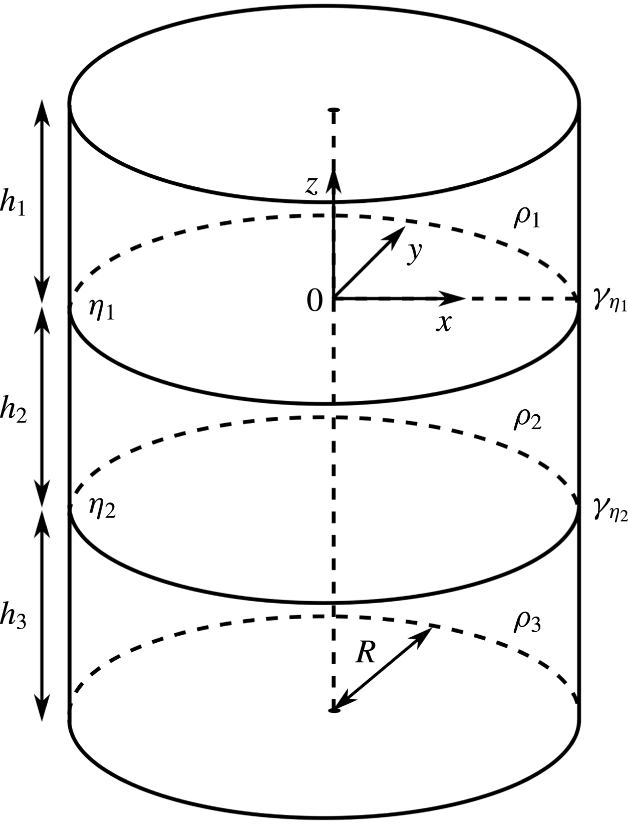
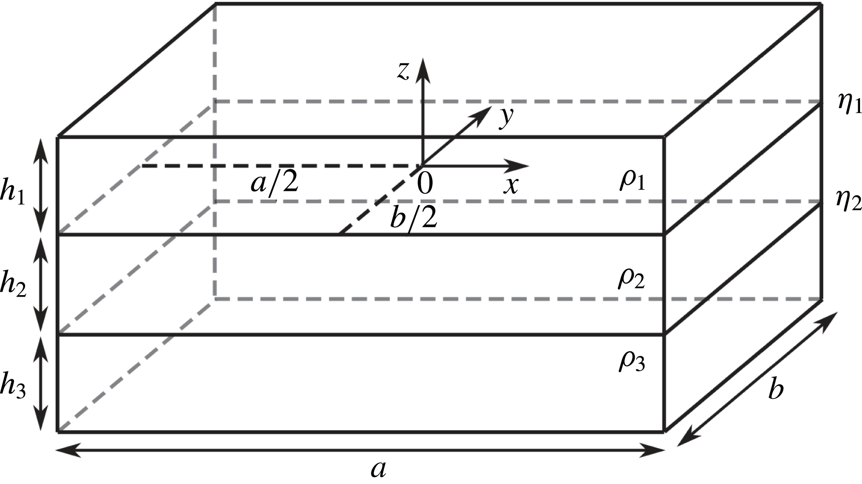
We apply the potential flow analysis to an ideal cylinder, as depicted in figure 2. The cylindrical geometry was chosen because it is a generic case. A cylindrical cell is always unstable (
 $\unicode[STIX]{x1D6FD}_{c}=0$
) in the inviscid limit (Lukyanov et al.
Reference Lukyanov, El and Molokov2001). Furthermore, there is no need to consider the influence of a horizontal aspect ratio on stability. Anyway, the theory described below is not restricted to cylinders but can be easily transferred to arbitrarily shaped vertical side walls. We show this on the example of a rectangular box in appendix A.
The cylindrical tank with the radius
 $R$
was defined to contain three immiscible phases
 $i=1,2,3$
of densities
 $\unicode[STIX]{x1D70C}_{i}$
and heights
 $h_{i}$
, where
 $\unicode[STIX]{x1D70C}_{1}<\unicode[STIX]{x1D70C}_{2}<\unicode[STIX]{x1D70C}_{3}$
has to be fulfilled to realize a stratified system. Two interfaces with interfacial tensions
 $\unicode[STIX]{x1D6FE}_{\unicode[STIX]{x1D702}_{1}}$
and
 $\unicode[STIX]{x1D6FE}_{\unicode[STIX]{x1D702}_{2}}$
are located at
 $z=\unicode[STIX]{x1D702}_{1}(x,y,t)$
and
 $z=\unicode[STIX]{x1D702}_{2}(x,y,t)$
. At this point we neglect interfacial tension effects at the side walls restricting the analysis to contact angles of
 $90^{\circ }$
and free-slip contact lines. The coordinate origin of the system is placed in the centre of the upper unperturbed interface
 $\unicode[STIX]{x1D702}_{1}$
.
Sketch of the idealized cylindrical three-layer system determined by the radius
 $R$
, three phases
 $i=1,2,3$
of densities
 $\unicode[STIX]{x1D70C}_{i}$
and heights
 $h_{i}$
as well as two interfaces
 $\unicode[STIX]{x1D702}_{1}$
and
 $\unicode[STIX]{x1D702}_{2}$
with corresponding interfacial tensions
 $\unicode[STIX]{x1D6FE}_{\unicode[STIX]{x1D702}_{1}}$
and
 $\unicode[STIX]{x1D6FE}_{\unicode[STIX]{x1D702}_{2}}$
.

To facilitate potential flow theory, a few simplifications have to be made. First, an inviscid flow has to be assumed, by which damping effects at the tank walls and on the interfaces are neglected. Actually, viscosity affects the natural frequencies of sloshing interfaces only very slightly (Ibrahim Reference Ibrahim2005) and can be neglected without problems in comparison to the pressure exchange forces basically determining the coupling dynamics. Secondly, the flow is supposed to be irrotational. That seems to be an counterintuitive assumption at first glance since the MPRI is driven by rotational Lorentz forces. By using this approximation, we completely neglect the rotational part of the flow that causes and drives the instability. Nevertheless, as mentioned before, the induced wave dynamics in the unstable regime can be well approximated by the irrotational part of the flow only. In § 3.2.1 it is shown that rotational Lorentz forces primarily influence the shape of the waves, but not their frequencies and amplitude ratios. Finally, the wave amplitudes are restricted to be sufficiently small to facilitate linear wave theory and all three fluids are treated as incompressible.
2.2 Potential flow analysis
Under the above simplifications the velocity fields
 $\boldsymbol{u}_{i}$
of all three phases
 $i=1,2,3$
can be expressed unambiguously by the gradient of scalar potentials
 $\unicode[STIX]{x1D719}_{i}$
as
 $$\begin{eqnarray}\boldsymbol{u}_{i}=\unicode[STIX]{x1D735}\unicode[STIX]{x1D719}_{i}.\end{eqnarray}$$
For fulfilling momentum and mass conservation, Bernoulli’s and Laplace’s equation have to be solved in all phases
 $$\begin{eqnarray}\displaystyle & \displaystyle {\displaystyle \frac{\unicode[STIX]{x2202}\unicode[STIX]{x1D719}_{i}}{\unicode[STIX]{x2202}t}}+{\displaystyle \frac{P_{i}}{\unicode[STIX]{x1D70C}_{i}}}+gz=c_{i}(t), & \displaystyle\end{eqnarray}$$
 $$\begin{eqnarray}\displaystyle & \displaystyle \unicode[STIX]{x0394}\unicode[STIX]{x1D719}_{i}=0, & \displaystyle\end{eqnarray}$$
where
 $P_{i}$
denotes the pressure,
 $g$
the standard acceleration due to gravity and
 $c_{i}(t)$
are arbitrary time-dependent integration constants. In addition, using cylindrical coordinates (
 $r,\unicode[STIX]{x1D711},z$
), the following sets of dynamic boundary conditions must be satisfied:
 $$\begin{eqnarray}\displaystyle & \displaystyle \text{top wall:}\quad {\displaystyle \frac{\unicode[STIX]{x2202}\unicode[STIX]{x1D719}_{1}}{\unicode[STIX]{x2202}z}}=0|_{z=h_{1}}, & \displaystyle\end{eqnarray}$$
 $$\begin{eqnarray}\displaystyle & \displaystyle \text{bottom wall:}\quad {\displaystyle \frac{\unicode[STIX]{x2202}\unicode[STIX]{x1D719}_{3}}{\unicode[STIX]{x2202}z}}=0|_{z=-(h_{2}+h_{3})}, & \displaystyle\end{eqnarray}$$
 $$\begin{eqnarray}\displaystyle & \displaystyle \text{side wall:}\quad {\displaystyle \frac{\unicode[STIX]{x2202}\unicode[STIX]{x1D719}_{1}}{\unicode[STIX]{x2202}r}}={\displaystyle \frac{\unicode[STIX]{x2202}\unicode[STIX]{x1D719}_{2}}{\unicode[STIX]{x2202}r}}={\displaystyle \frac{\unicode[STIX]{x2202}\unicode[STIX]{x1D719}_{3}}{\unicode[STIX]{x2202}r}}=0|_{r=R}, & \displaystyle\end{eqnarray}$$
 $$\begin{eqnarray}\displaystyle & \displaystyle \text{upper interface:}\quad {\displaystyle \frac{\unicode[STIX]{x2202}\unicode[STIX]{x1D719}_{1}}{\unicode[STIX]{x2202}z}}={\displaystyle \frac{\unicode[STIX]{x2202}\unicode[STIX]{x1D719}_{2}}{\unicode[STIX]{x2202}z}}\bigg|_{z=\unicode[STIX]{x1D702}_{1}}, & \displaystyle\end{eqnarray}$$
 $$\begin{eqnarray}\displaystyle & \displaystyle \text{lower interface:}\quad {\displaystyle \frac{\unicode[STIX]{x2202}\unicode[STIX]{x1D719}_{2}}{\unicode[STIX]{x2202}z}}={\displaystyle \frac{\unicode[STIX]{x2202}\unicode[STIX]{x1D719}_{3}}{\unicode[STIX]{x2202}z}}\bigg|_{z=\unicode[STIX]{x1D702}_{2}}. & \displaystyle\end{eqnarray}$$
No-outflow boundary conditions were formulated at the side wall
 $r=R$
(2.6), at the top
 $z=h_{1}$
(2.4) and the bottom wall
 $z=-(h_{2}+h_{3})$
(2.5), while conditions (2.7) and (2.8) ensure interface preservation. By assuming a harmonic time dependency
 $\unicode[STIX]{x1D719}_{i}\sim \cos (\unicode[STIX]{x1D714}t)$
, where
 $\unicode[STIX]{x1D714}$
marks the angular frequency, potential solutions for the Laplace equations (2.3) in cylindrical coordinates fulfilling all above conditions can be found as superpositions of infinite wave modes
 $m\in \mathbb{N}_{0}$
and
 $n\in \mathbb{N}_{1}$
:
 $$\begin{eqnarray}\displaystyle \unicode[STIX]{x1D719}_{1}(r,\unicode[STIX]{x1D711},z,t) & = & \displaystyle -\mathop{\sum }_{m=0}^{\infty }\mathop{\sum }_{n=1}^{\infty }\tilde{\unicode[STIX]{x1D702}}_{1}^{mn}{\displaystyle \frac{\cosh \left({\displaystyle \frac{\unicode[STIX]{x1D716}_{mn}}{R}}(z-h_{1})\right)}{\sinh \left({\displaystyle \frac{\unicode[STIX]{x1D716}_{mn}}{R}}(h_{1})\right)}}\text{J}_{m}\left(\unicode[STIX]{x1D716}_{mn}{\displaystyle \frac{r}{R}}\right)\cos (m\unicode[STIX]{x1D711}-\unicode[STIX]{x1D714}t),\end{eqnarray}$$
 $$\begin{eqnarray}\displaystyle \unicode[STIX]{x1D719}_{2}(r,\unicode[STIX]{x1D711},z,t) & = & \displaystyle \mathop{\sum }_{m=0}^{\infty }\mathop{\sum }_{n=1}^{\infty }\left[\tilde{\unicode[STIX]{x1D702}}_{1}^{mn}\left(\text{e}^{{\displaystyle \frac{\unicode[STIX]{x1D716}_{mn}}{R}}h_{2}}\cosh \left({\displaystyle \frac{\unicode[STIX]{x1D716}_{mn}}{R}}z\right)-\text{e}^{-{\displaystyle \frac{\unicode[STIX]{x1D716}_{mn}}{R}}z}\sinh \left({\displaystyle \frac{\unicode[STIX]{x1D716}_{mn}}{R}}h_{2}\right)\right)\right.\nonumber\\ \displaystyle & & \displaystyle \left.-\,\tilde{\unicode[STIX]{x1D702}}_{2}^{mn}\cosh \vphantom{\frac{\mathop{\sum }_{\int }}{\mathop{\sum }_{\int }}}\left({\displaystyle \frac{\unicode[STIX]{x1D716}_{mn}}{R}}z\right)\right]\cdot {\displaystyle \frac{1}{\sinh \left({\displaystyle \frac{\unicode[STIX]{x1D716}_{mn}}{R}}h_{2}\right)}}\text{J}_{m}\left(\unicode[STIX]{x1D716}_{mn}{\displaystyle \frac{r}{R}}\right)\cos (m\unicode[STIX]{x1D711}-\unicode[STIX]{x1D714}t),\qquad\end{eqnarray}$$
 $$\begin{eqnarray}\displaystyle \unicode[STIX]{x1D719}_{3}(r,\unicode[STIX]{x1D711},z,t) & = & \displaystyle \mathop{\sum }_{m=0}^{\infty }\mathop{\sum }_{n=1}^{\infty }\tilde{\unicode[STIX]{x1D702}}_{2}^{mn}{\displaystyle \frac{\cosh \left({\displaystyle \frac{\unicode[STIX]{x1D716}_{mn}}{R}}(z+h_{2}+h_{3})\right)}{\sinh \left({\displaystyle \frac{\unicode[STIX]{x1D716}_{mn}}{R}}(h_{3})\right)}}\text{J}_{m}\left(\unicode[STIX]{x1D716}_{mn}{\displaystyle \frac{r}{R}}\right)\cos (m\unicode[STIX]{x1D711}-\unicode[STIX]{x1D714}t).\qquad\end{eqnarray}$$
 $\text{J}_{m}$
denotes the
 $m$
th-order Bessel function of the first kind and
 $\tilde{\unicode[STIX]{x1D702}}_{1}^{mn}$
as well as
 $\tilde{\unicode[STIX]{x1D702}}_{2}^{mn}$
the mode-dependent amplitudes of the upper and lower interface.
 $m$
is often called the azimuthal wavenumber because it only appears in the cosine terms and for
 $m=0$
all solutions are radial symmetric.
 $\unicode[STIX]{x1D716}_{mn}$
mark the radial wavenumbers, which are restricted to the
 $n$
roots of the first derivative of the
 $m$
th-order Bessel function
 $$\begin{eqnarray}\text{J}_{m}^{\prime }(\unicode[STIX]{x1D716}_{mn})=0,\end{eqnarray}$$
to fulfil the radial no-outflow boundary condition. The roots can be easily determined numerically or found in, e.g. Abramowitz & Stegun (Reference Abramowitz and Stegun1972). Exploiting the fact that the vertical velocity on the interfaces is identical to its linearized time variation
 $$\begin{eqnarray}\left.{\displaystyle \frac{\unicode[STIX]{x2202}\unicode[STIX]{x1D702}_{1}}{\unicode[STIX]{x2202}t}}={\displaystyle \frac{\unicode[STIX]{x2202}\unicode[STIX]{x1D719}_{1}}{\unicode[STIX]{x2202}z}}={\displaystyle \frac{\unicode[STIX]{x2202}\unicode[STIX]{x1D719}_{2}}{\unicode[STIX]{x2202}z}}\right|_{z=0}\quad \text{and}\quad \left.{\displaystyle \frac{\unicode[STIX]{x2202}\unicode[STIX]{x1D702}_{2}}{\unicode[STIX]{x2202}t}}={\displaystyle \frac{\unicode[STIX]{x2202}\unicode[STIX]{x1D719}_{2}}{\unicode[STIX]{x2202}z}}={\displaystyle \frac{\unicode[STIX]{x2202}\unicode[STIX]{x1D719}_{3}}{\unicode[STIX]{x2202}z}}\right|_{z=-h_{2}},\end{eqnarray}$$
the interfacial shapes can be easily derived from the scalar flow potentials as:
 $$\begin{eqnarray}\displaystyle \unicode[STIX]{x1D702}_{1}(r,\unicode[STIX]{x1D711},t) & = & \displaystyle \mathop{\sum }_{m=0}^{\infty }\mathop{\sum }_{n=1}^{\infty }\tilde{\unicode[STIX]{x1D702}}_{1}^{mn}{\displaystyle \frac{\unicode[STIX]{x1D716}_{mn}}{R\unicode[STIX]{x1D714}}}\text{J}_{m}\left(\unicode[STIX]{x1D716}_{mn}{\displaystyle \frac{r}{R}}\right)\cos (m\unicode[STIX]{x1D711}-\unicode[STIX]{x1D714}t),\end{eqnarray}$$
 $$\begin{eqnarray}\displaystyle \unicode[STIX]{x1D702}_{2}(r,\unicode[STIX]{x1D711},t) & = & \displaystyle \mathop{\sum }_{m=0}^{\infty }\mathop{\sum }_{n=1}^{\infty }\tilde{\unicode[STIX]{x1D702}}_{2}^{mn}{\displaystyle \frac{\unicode[STIX]{x1D716}_{mn}}{R\unicode[STIX]{x1D714}}}\text{J}_{m}\left(\unicode[STIX]{x1D716}_{mn}{\displaystyle \frac{r}{R}}\right)\cos (m\unicode[STIX]{x1D711}-\unicode[STIX]{x1D714}t).\end{eqnarray}$$
 $\text{Mg}\Vert \text{Sb}$
LMB (Weber et al.
Reference Weber, Beckstein, Herreman, Horstmann, Nore, Stefani and Weier2017b
) that in many cases the
 $m=n=1$
mode giving
 $\unicode[STIX]{x1D716}_{11}\approx 1.841$
becomes most unstable by the MPRI. This mode corresponds to the rolling tilted interface sketched in figure 1. Now, the wave frequencies can be determined by regarding the dynamic boundary condition, which claims that the pressure drop
 $\unicode[STIX]{x0394}P$
at the interfaces has to be balanced by the surface tensions
 $\unicode[STIX]{x1D6FE}_{\unicode[STIX]{x1D702}_{1}}$
and
 $\unicode[STIX]{x1D6FE}_{\unicode[STIX]{x1D702}_{2}}$
. The pressure of each phase is determined by the Bernoulli equation (2.2), whereby the pressure drops can be expressed with
 $$\begin{eqnarray}\displaystyle \unicode[STIX]{x0394}P|_{\unicode[STIX]{x1D702}_{1}} & = & \displaystyle P_{2}|_{\unicode[STIX]{x1D702}_{1}}-P_{1}|_{\unicode[STIX]{x1D702}_{1}}=-\unicode[STIX]{x1D70C}_{2}{\displaystyle \frac{\unicode[STIX]{x2202}\unicode[STIX]{x1D719}_{2}}{\unicode[STIX]{x2202}t}}\bigg|_{\unicode[STIX]{x1D702}_{1}}-\unicode[STIX]{x1D70C}_{2}g\unicode[STIX]{x1D702}_{1}+\unicode[STIX]{x1D70C}_{1}{\displaystyle \frac{\unicode[STIX]{x2202}\unicode[STIX]{x1D719}_{1}}{\unicode[STIX]{x2202}t}}\bigg|_{\unicode[STIX]{x1D702}_{1}}+\unicode[STIX]{x1D70C}_{1}g\unicode[STIX]{x1D702}_{1},\end{eqnarray}$$
 $$\begin{eqnarray}\displaystyle \unicode[STIX]{x0394}P|_{\unicode[STIX]{x1D702}_{2}} & = & \displaystyle P_{3}|_{\unicode[STIX]{x1D702}_{2}}-P_{2}|_{\unicode[STIX]{x1D702}_{2}}=-\unicode[STIX]{x1D70C}_{3}{\displaystyle \frac{\unicode[STIX]{x2202}\unicode[STIX]{x1D719}_{3}}{\unicode[STIX]{x2202}t}}\bigg|_{\unicode[STIX]{x1D702}_{2}}-\unicode[STIX]{x1D70C}_{3}g\unicode[STIX]{x1D702}_{2}+\unicode[STIX]{x1D70C}_{2}{\displaystyle \frac{\unicode[STIX]{x2202}\unicode[STIX]{x1D719}_{2}}{\unicode[STIX]{x2202}t}}\bigg|_{\unicode[STIX]{x1D702}_{2}}+\unicode[STIX]{x1D70C}_{2}g\unicode[STIX]{x1D702}_{2}.\end{eqnarray}$$
 $c_{i}(t)$
were incorporated into the flow potentials
 $\unicode[STIX]{x1D719}_{i}$
. The pressure drops due to surface tension are described in dependence on the principle radii of curvature
 $R_{1}$
and
 $R_{2}$
by the Young–Laplace equation
 $$\begin{eqnarray}\displaystyle \unicode[STIX]{x0394}P|_{\unicode[STIX]{x1D702}_{1}} & = & \displaystyle \unicode[STIX]{x1D6FE}_{\unicode[STIX]{x1D702}_{1}}\left({\displaystyle \frac{1}{R_{1}}}+{\displaystyle \frac{1}{R_{2}}}\right)\bigg|_{\unicode[STIX]{x1D702}_{1}},\end{eqnarray}$$
 $$\begin{eqnarray}\displaystyle \unicode[STIX]{x0394}P|_{\unicode[STIX]{x1D702}_{2}} & = & \displaystyle \unicode[STIX]{x1D6FE}_{\unicode[STIX]{x1D702}_{2}}\left({\displaystyle \frac{1}{R_{1}}}+{\displaystyle \frac{1}{R_{2}}}\right)\bigg|_{\unicode[STIX]{x1D702}_{2}}.\end{eqnarray}$$
 $$\begin{eqnarray}{\displaystyle \frac{1}{R_{1}}}\bigg|_{\unicode[STIX]{x1D702}_{j}}\approx {\displaystyle \frac{\unicode[STIX]{x2202}^{2}\unicode[STIX]{x1D702}_{j}}{\unicode[STIX]{x2202}x^{2}}},\quad {\displaystyle \frac{1}{R_{2}}}\bigg|_{\unicode[STIX]{x1D702}_{j}}\approx {\displaystyle \frac{\unicode[STIX]{x2202}^{2}\unicode[STIX]{x1D702}_{j}}{\unicode[STIX]{x2202}y^{2}}}\quad \text{with }j=1,2.\end{eqnarray}$$
By now, the dynamic boundary condition can be expressed in dependence on the flow potentials
 $\unicode[STIX]{x1D719}_{i}$
by calculating the first time derivatives of (2.13a
), exploiting the preservation conditions (2.11) and eliminating the pressure drops. One gets
 $$\begin{eqnarray}\displaystyle & & \displaystyle \left.\unicode[STIX]{x1D70C}_{1}{\displaystyle \frac{\unicode[STIX]{x2202}^{2}\unicode[STIX]{x1D719}_{1}}{\unicode[STIX]{x2202}t^{2}}}+\unicode[STIX]{x1D70C}_{1}g{\displaystyle \frac{\unicode[STIX]{x2202}\unicode[STIX]{x1D719}_{1}}{\unicode[STIX]{x2202}z}}=\unicode[STIX]{x1D70C}_{2}{\displaystyle \frac{\unicode[STIX]{x2202}^{2}\unicode[STIX]{x1D719}_{2}}{\unicode[STIX]{x2202}t^{2}}}+\unicode[STIX]{x1D70C}_{2}g{\displaystyle \frac{\unicode[STIX]{x2202}\unicode[STIX]{x1D719}_{2}}{\unicode[STIX]{x2202}z}}-\unicode[STIX]{x1D6FE}_{\unicode[STIX]{x1D702}_{1}}\left({\displaystyle \frac{\unicode[STIX]{x2202}^{2}}{\unicode[STIX]{x2202}x^{2}}}+{\displaystyle \frac{\unicode[STIX]{x2202}^{2}}{\unicode[STIX]{x2202}y^{2}}}\right){\displaystyle \frac{\unicode[STIX]{x2202}\unicode[STIX]{x1D719}_{2}}{\unicode[STIX]{x2202}z}}\right|_{z=\unicode[STIX]{x1D702}_{1}},\quad\end{eqnarray}$$
 $$\begin{eqnarray}\displaystyle & & \displaystyle \left.\unicode[STIX]{x1D70C}_{2}{\displaystyle \frac{\unicode[STIX]{x2202}^{2}\unicode[STIX]{x1D719}_{2}}{\unicode[STIX]{x2202}t^{2}}}+\unicode[STIX]{x1D70C}_{2}g{\displaystyle \frac{\unicode[STIX]{x2202}\unicode[STIX]{x1D719}_{2}}{\unicode[STIX]{x2202}z}}=\unicode[STIX]{x1D70C}_{3}{\displaystyle \frac{\unicode[STIX]{x2202}^{2}\unicode[STIX]{x1D719}_{3}}{\unicode[STIX]{x2202}t^{2}}}+\unicode[STIX]{x1D70C}_{3}g{\displaystyle \frac{\unicode[STIX]{x2202}\unicode[STIX]{x1D719}_{3}}{\unicode[STIX]{x2202}z}}-\unicode[STIX]{x1D6FE}_{\unicode[STIX]{x1D702}_{2}}\left({\displaystyle \frac{\unicode[STIX]{x2202}^{2}}{\unicode[STIX]{x2202}x^{2}}}+{\displaystyle \frac{\unicode[STIX]{x2202}^{2}}{\unicode[STIX]{x2202}y^{2}}}\right){\displaystyle \frac{\unicode[STIX]{x2202}\unicode[STIX]{x1D719}_{3}}{\unicode[STIX]{x2202}z}}\right|_{z=\unicode[STIX]{x1D702}_{2}}.\end{eqnarray}$$
 $$\begin{eqnarray}{\displaystyle \frac{\unicode[STIX]{x2202}^{2}\unicode[STIX]{x1D719}_{i}}{\unicode[STIX]{x2202}z^{2}}}=-\left({\displaystyle \frac{\unicode[STIX]{x2202}^{2}\unicode[STIX]{x1D719}_{i}}{\unicode[STIX]{x2202}x^{2}}}+{\displaystyle \frac{\unicode[STIX]{x2202}^{2}\unicode[STIX]{x1D719}_{i}}{\unicode[STIX]{x2202}y^{2}}}\right)\end{eqnarray}$$
so that the kinematic boundary conditions finally read
 $$\begin{eqnarray}\displaystyle & & \displaystyle \left.\unicode[STIX]{x1D70C}_{1}{\displaystyle \frac{\unicode[STIX]{x2202}^{2}\unicode[STIX]{x1D719}_{1}}{\unicode[STIX]{x2202}t^{2}}}+\unicode[STIX]{x1D70C}_{1}g{\displaystyle \frac{\unicode[STIX]{x2202}\unicode[STIX]{x1D719}_{1}}{\unicode[STIX]{x2202}z}}=\unicode[STIX]{x1D70C}_{2}{\displaystyle \frac{\unicode[STIX]{x2202}^{2}\unicode[STIX]{x1D719}_{2}}{\unicode[STIX]{x2202}t^{2}}}+\unicode[STIX]{x1D70C}_{2}g{\displaystyle \frac{\unicode[STIX]{x2202}\unicode[STIX]{x1D719}_{2}}{\unicode[STIX]{x2202}z}}+\unicode[STIX]{x1D6FE}_{\unicode[STIX]{x1D702}_{1}}{\displaystyle \frac{\unicode[STIX]{x2202}^{3}\unicode[STIX]{x1D719}_{2}}{\unicode[STIX]{x2202}z^{3}}}\right|_{z=\unicode[STIX]{x1D702}_{1}},\end{eqnarray}$$
 $$\begin{eqnarray}\displaystyle & & \displaystyle \left.\unicode[STIX]{x1D70C}_{2}{\displaystyle \frac{\unicode[STIX]{x2202}^{2}\unicode[STIX]{x1D719}_{2}}{\unicode[STIX]{x2202}t^{2}}}+\unicode[STIX]{x1D70C}_{2}g{\displaystyle \frac{\unicode[STIX]{x2202}\unicode[STIX]{x1D719}_{2}}{\unicode[STIX]{x2202}z}}=\unicode[STIX]{x1D70C}_{3}{\displaystyle \frac{\unicode[STIX]{x2202}^{2}\unicode[STIX]{x1D719}_{3}}{\unicode[STIX]{x2202}t^{2}}}+\unicode[STIX]{x1D70C}_{3}g{\displaystyle \frac{\unicode[STIX]{x2202}\unicode[STIX]{x1D719}_{3}}{\unicode[STIX]{x2202}z}}+\unicode[STIX]{x1D6FE}_{\unicode[STIX]{x1D702}_{2}}{\displaystyle \frac{\unicode[STIX]{x2202}^{3}\unicode[STIX]{x1D719}_{3}}{\unicode[STIX]{x2202}z^{3}}}\right|_{z=\unicode[STIX]{x1D702}_{2}}.\end{eqnarray}$$
 $x$
- and
 $y$
-coordinate dependency has been eliminated. Finally, two dispersion relations
 $\unicode[STIX]{x1D714}(\unicode[STIX]{x1D716}_{mn})$
connected to both interfaces are derived by inserting the potential solutions (2.9) into (2.18):
 $$\begin{eqnarray}\displaystyle \unicode[STIX]{x1D714}_{1|2mn}^{2} & = & \displaystyle {\displaystyle \frac{(\unicode[STIX]{x1D70C}_{2}-\unicode[STIX]{x1D70C}_{1})g{\displaystyle \frac{\unicode[STIX]{x1D716}_{mn}}{R}}+\unicode[STIX]{x1D6FE}_{\unicode[STIX]{x1D702}_{1}}\left({\displaystyle \frac{\unicode[STIX]{x1D716}_{mn}}{R}}\right)^{3}}{\unicode[STIX]{x1D70C}_{1}\coth \left({\displaystyle \frac{\unicode[STIX]{x1D716}_{mn}}{R}}h_{1}\right)+\unicode[STIX]{x1D70C}_{2}\left(\coth \left({\displaystyle \frac{\unicode[STIX]{x1D716}_{mn}}{R}}h_{2}\right)-{\displaystyle \frac{\tilde{\unicode[STIX]{x1D702}}_{2}^{mn}}{\tilde{\unicode[STIX]{x1D702}}_{1}^{mn}}}{\displaystyle \frac{1}{\sinh \left({\displaystyle \frac{\unicode[STIX]{x1D716}_{mn}}{R}}h_{2}\right)}}\right)}},\end{eqnarray}$$
 $$\begin{eqnarray}\displaystyle \unicode[STIX]{x1D714}_{2|3mn}^{2} & = & \displaystyle {\displaystyle \frac{(\unicode[STIX]{x1D70C}_{3}-\unicode[STIX]{x1D70C}_{2})g{\displaystyle \frac{\unicode[STIX]{x1D716}_{mn}}{R}}+\unicode[STIX]{x1D6FE}_{\unicode[STIX]{x1D702}_{2}}\left({\displaystyle \frac{\unicode[STIX]{x1D716}_{mn}}{R}}\right)^{3}}{\unicode[STIX]{x1D70C}_{3}\coth \left({\displaystyle \frac{\unicode[STIX]{x1D716}_{mn}}{R}}h_{3}\right)+\unicode[STIX]{x1D70C}_{2}\left(\coth \left({\displaystyle \frac{\unicode[STIX]{x1D716}_{mn}}{R}}h_{2}\right)-{\displaystyle \frac{\tilde{\unicode[STIX]{x1D702}}_{1}^{mn}}{\tilde{\unicode[STIX]{x1D702}}_{2}^{mn}}}{\displaystyle \frac{1}{\sinh \left({\displaystyle \frac{\unicode[STIX]{x1D716}_{mn}}{R}}h_{2}\right)}}\right)}}.\end{eqnarray}$$
 $\tilde{\unicode[STIX]{x1D702}}_{1}^{mn}/\tilde{\unicode[STIX]{x1D702}}_{2}^{mn}$
and
 $\tilde{\unicode[STIX]{x1D702}}_{2}^{mn}/\tilde{\unicode[STIX]{x1D702}}_{1}^{mn}$
. Eliminating them leads to a fourth-order dispersion relation
 $$\begin{eqnarray}\displaystyle \left.\begin{array}{@{}l@{}}a\unicode[STIX]{x1D714}^{4}+b\unicode[STIX]{x1D714}^{2}+c=0,\quad \text{with}\\ a=\left(\unicode[STIX]{x1D70C}_{2}\coth \left({\displaystyle \frac{\unicode[STIX]{x1D716}_{mn}}{R}}h_{2}\right)+\unicode[STIX]{x1D70C}_{3}\coth \left({\displaystyle \frac{\unicode[STIX]{x1D716}_{mn}}{R}}h_{3}\right)\right)\left(\unicode[STIX]{x1D70C}_{2}\coth \left({\displaystyle \frac{\unicode[STIX]{x1D716}_{mn}}{R}}h_{2}\right)+\unicode[STIX]{x1D70C}_{1}\coth \left({\displaystyle \frac{\unicode[STIX]{x1D716}_{mn}}{R}}h_{1}\right)\right)\\ \quad \quad -{\displaystyle \frac{\unicode[STIX]{x1D70C}_{2}^{2}}{\sinh \left({\displaystyle \frac{\unicode[STIX]{x1D716}_{mn}}{R}}h_{2}\right)^{2}}},\\ b=-\left((\unicode[STIX]{x1D70C}_{2}-\unicode[STIX]{x1D70C}_{1})g{\displaystyle \frac{\unicode[STIX]{x1D716}_{mn}}{R}}+\unicode[STIX]{x1D6FE}_{\unicode[STIX]{x1D702}_{1}}\left({\displaystyle \frac{\unicode[STIX]{x1D716}_{mn}}{R}}\right)^{3}\right)\left(\unicode[STIX]{x1D70C}_{2}\coth \left({\displaystyle \frac{\unicode[STIX]{x1D716}_{mn}}{R}}h_{2}\right)+\unicode[STIX]{x1D70C}_{3}\coth \left({\displaystyle \frac{\unicode[STIX]{x1D716}_{mn}}{R}}h_{3}\right)\right)\\ \quad \quad -\left((\unicode[STIX]{x1D70C}_{3}-\unicode[STIX]{x1D70C}_{2})g{\displaystyle \frac{\unicode[STIX]{x1D716}_{mn}}{R}}+\unicode[STIX]{x1D6FE}_{\unicode[STIX]{x1D702}_{2}}\left({\displaystyle \frac{\unicode[STIX]{x1D716}_{mn}}{R}}\right)^{3}\right)\left(\unicode[STIX]{x1D70C}_{2}\coth \left({\displaystyle \frac{\unicode[STIX]{x1D716}_{mn}}{R}}h_{2}\right)+\unicode[STIX]{x1D70C}_{1}\coth \left({\displaystyle \frac{\unicode[STIX]{x1D716}_{mn}}{R}}h_{1}\right)\right),\\ c=\left((\unicode[STIX]{x1D70C}_{2}-\unicode[STIX]{x1D70C}_{1})g{\displaystyle \frac{\unicode[STIX]{x1D716}_{mn}}{R}}+\unicode[STIX]{x1D6FE}_{\unicode[STIX]{x1D702}_{1}}\left({\displaystyle \frac{\unicode[STIX]{x1D716}_{mn}}{R}}\right)^{3}\right)\left((\unicode[STIX]{x1D70C}_{3}-\unicode[STIX]{x1D70C}_{2})g{\displaystyle \frac{\unicode[STIX]{x1D716}_{mn}}{R}}+\unicode[STIX]{x1D6FE}_{\unicode[STIX]{x1D702}_{2}}\left({\displaystyle \frac{\unicode[STIX]{x1D716}_{mn}}{R}}\right)^{3}\right),\end{array}\right\} & & \displaystyle \nonumber\\ \displaystyle & & \displaystyle\end{eqnarray}$$
which provides two independent analytical solutions
 $$\begin{eqnarray}\unicode[STIX]{x1D714}_{\pm }^{2}={\displaystyle \frac{-b\pm \sqrt{b^{2}-4ac}}{2a}}.\end{eqnarray}$$
Consequently, in contrast to two-layer ARCs, LMBs involve always two eigenfrequencies
 $\unicode[STIX]{x1D714}_{+}$
and
 $\unicode[STIX]{x1D714}_{-}$
. It can be seen readily from (2.21) that
 $\unicode[STIX]{x1D714}_{+}$
is always larger than
 $\unicode[STIX]{x1D714}_{-}$
. Hence, in analogy to the coupled harmonic oscillator,
 $\unicode[STIX]{x1D714}_{+}$
is called the fast mode and
 $\unicode[STIX]{x1D714}_{-}$
the slow mode, respectively. Note that Weber et al. (Reference Weber, Beckstein, Herreman, Horstmann, Nore, Stefani and Weier2017b
) gave the dispersion relation (2.21) for the specific case of
 $\text{Mg}\Vert \text{Sb}$
cells.
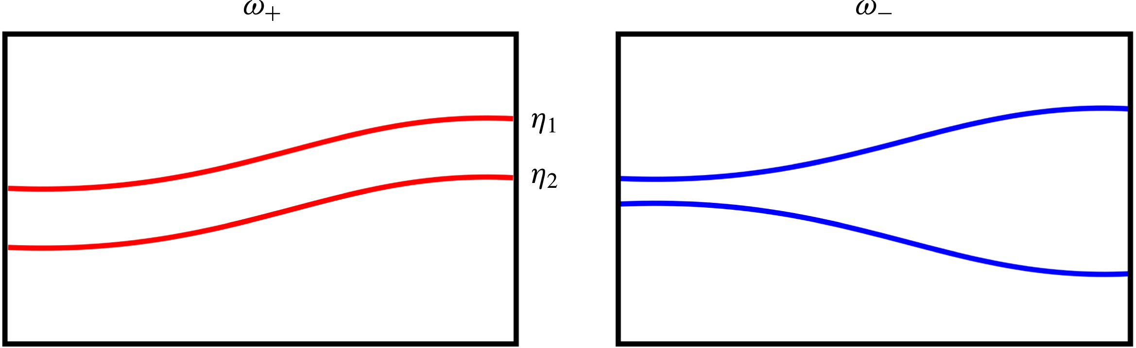
Schematic of the symmetric fast mode
 $\unicode[STIX]{x1D714}_{+}$
(red) and the antisymmetric slow mode
 $\unicode[STIX]{x1D714}_{-}$
(blue) of the wavenumber
 $\unicode[STIX]{x1D716}_{11}$
in cross-section.

Moreover, by knowing the frequency solutions from (2.21), the amplitude ratios can be analytically determined by transposing (2.19a ) or (2.19b ) giving
 $$\begin{eqnarray}\displaystyle {\displaystyle \frac{\tilde{\unicode[STIX]{x1D702}}_{1}^{mn}}{\tilde{\unicode[STIX]{x1D702}}_{2}^{mn}}}_{\pm } & = & \displaystyle {\displaystyle \frac{\sinh \left({\displaystyle \frac{\unicode[STIX]{x1D716}_{mn}}{R}}h_{2}\right)}{\unicode[STIX]{x1D70C}_{2}}}\left[\vphantom{\frac{\mathop{\sum }_{\int }}{\mathop{\sum }_{\int }^{2}}}\unicode[STIX]{x1D70C}_{2}\coth \left({\displaystyle \frac{\unicode[STIX]{x1D716}_{mn}}{R}}h_{2}\right)+\unicode[STIX]{x1D70C}_{3}\coth \left({\displaystyle \frac{\unicode[STIX]{x1D716}_{mn}}{R}}h_{3}\right)\right.\nonumber\\ \displaystyle & & \displaystyle -\,\left.{\displaystyle \frac{(\unicode[STIX]{x1D70C}_{3}-\unicode[STIX]{x1D70C}_{2})g{\displaystyle \frac{\unicode[STIX]{x1D716}_{mn}}{R}}+\unicode[STIX]{x1D6FE}_{\unicode[STIX]{x1D702}_{2}}\left({\displaystyle \frac{\unicode[STIX]{x1D716}_{mn}}{R}}\right)^{3}}{\unicode[STIX]{x1D714}_{\pm }^{2}}}\right].\end{eqnarray}$$
Corresponding to the two frequency solutions, we also find two different amplitude ratios, whereby it can readily be shown from (2.22) that for the plus mode the amplitude ratio is always positive and for the minus mode always negative
 $$\begin{eqnarray}{\displaystyle \frac{\tilde{\unicode[STIX]{x1D702}}_{1}^{mn}}{\tilde{\unicode[STIX]{x1D702}}_{2}^{mn}}}_{+}>0,\quad {\displaystyle \frac{\tilde{\unicode[STIX]{x1D702}}_{1}^{mn}}{\tilde{\unicode[STIX]{x1D702}}_{2}^{mn}}}_{-}<0.\end{eqnarray}$$
From that directly follows that in the plus mode the interfaces propagate symmetrically (in phase) and in the minus mode antisymmetrically (with a
 $180^{\circ }$
phase shift). Exemplarily, both coupling states are schematically sketched in figure 3.
To conclude, we have to distinguish between two essential coupling modes, the one fast and symmetric and the other slow and antisymmetric. Both modes may occur in LMBs having different consequences for the operation stability. This result is well known from the coupled harmonic oscillator and was to be reproduced since we employed linear wave theory. However, the formulas (2.21) and (2.22) now allow us to study the natural frequencies and the coupling dynamics in dependence on nine geometrical cell parameters and material properties
 $\unicode[STIX]{x1D70C}_{1},\unicode[STIX]{x1D70C}_{2},\unicode[STIX]{x1D70C}_{3},\unicode[STIX]{x1D6FE}_{\unicode[STIX]{x1D702}_{1}},\unicode[STIX]{x1D6FE}_{\unicode[STIX]{x1D702}_{2}},h_{1},h_{2},h_{3},R$
as presented in the next section.
2.3 Analysis of the coupling dynamics
In the following we analyse the strength of the interfacial wave coupling to predict in which parameter regimes the battery can be considered as decoupled and two-layer analysis to be sufficient to understand the MPRI, and in which regimes the wave coupling has a large share in the instability mechanism.
At fist we compare the expressions (2.19a
) and (2.19b
) of the three-layer dispersion relation with the corresponding two-layer dispersion relations
 $\unicode[STIX]{x1D714}_{\unicode[STIX]{x1D702}_{1}}$
and
 $\unicode[STIX]{x1D714}_{\unicode[STIX]{x1D702}_{2}}$
of both interfaces
 $\unicode[STIX]{x1D702}_{1}$
and
 $\unicode[STIX]{x1D702}_{2}$
that can be analogously derived and are given by
 $$\begin{eqnarray}\displaystyle & & \displaystyle \unicode[STIX]{x1D714}_{\unicode[STIX]{x1D702}_{1}}^{2}={\displaystyle \frac{(\unicode[STIX]{x1D70C}_{2}-\unicode[STIX]{x1D70C}_{1})g{\displaystyle \frac{\unicode[STIX]{x1D716}_{mn}}{R}}+\unicode[STIX]{x1D6FE}_{\unicode[STIX]{x1D702}_{1}}\left({\displaystyle \frac{\unicode[STIX]{x1D716}_{mn}}{R}}\right)^{3}}{\unicode[STIX]{x1D70C}_{1}\coth \left({\displaystyle \frac{\unicode[STIX]{x1D716}_{mn}}{R}}h_{1}\right)+\unicode[STIX]{x1D70C}_{2}\coth \left({\displaystyle \frac{\unicode[STIX]{x1D716}_{mn}}{R}}h_{2}\right)}},\end{eqnarray}$$
 $$\begin{eqnarray}\displaystyle & & \displaystyle \unicode[STIX]{x1D714}_{\unicode[STIX]{x1D702}_{2}}^{2}={\displaystyle \frac{(\unicode[STIX]{x1D70C}_{3}-\unicode[STIX]{x1D70C}_{2})g{\displaystyle \frac{\unicode[STIX]{x1D716}_{mn}}{R}}+\unicode[STIX]{x1D6FE}_{\unicode[STIX]{x1D702}_{2}}\left({\displaystyle \frac{\unicode[STIX]{x1D716}_{mn}}{R}}\right)^{3}}{\unicode[STIX]{x1D70C}_{2}\coth \left({\displaystyle \frac{\unicode[STIX]{x1D716}_{mn}}{R}}h_{2}\right)+\unicode[STIX]{x1D70C}_{3}\coth \left({\displaystyle \frac{\unicode[STIX]{x1D716}_{mn}}{R}}h_{3}\right)}}.\end{eqnarray}$$
 $$\begin{eqnarray}{\displaystyle \frac{\tilde{\unicode[STIX]{x1D702}}_{2}^{mn}}{\tilde{\unicode[STIX]{x1D702}}_{1}^{mn}}}{\displaystyle \frac{1}{\sinh \left({\displaystyle \frac{\unicode[STIX]{x1D716}_{mn}}{R}}h_{2}\right)}}\quad \text{or}\quad {\displaystyle \frac{\tilde{\unicode[STIX]{x1D702}}_{1}^{mn}}{\tilde{\unicode[STIX]{x1D702}}_{2}^{mn}}}{\displaystyle \frac{1}{\sinh \left({\displaystyle \frac{\unicode[STIX]{x1D716}_{mn}}{R}}h_{2}\right)}},\end{eqnarray}$$
respectively. These terms can be exploited to make first estimations in which cases the battery can be considered as decoupled. The terms are vanishing for two different limits: on the one hand if the salt layer height
 $h_{2}$
is becoming large in comparison to the radius
 $R$
. In that limit both interfaces are placed too far apart from each other to interact and are both propagating in their own two-layer eigenfrequency
 $\unicode[STIX]{x1D714}_{\unicode[STIX]{x1D702}_{1}}$
and
 $\unicode[STIX]{x1D714}_{\unicode[STIX]{x1D702}_{2}}$
. Effectively, this limit is not practically relevant for LMBs since the salt layer should always be as thin as possible to realize maximum efficiency. More important is the second limit, where the amplitude ratio is becoming sufficiently small or large
 $$\begin{eqnarray}{\displaystyle \frac{\tilde{\unicode[STIX]{x1D702}}_{1}^{mn}}{\tilde{\unicode[STIX]{x1D702}}_{2}^{mn}}}\gg 1\quad \text{or}\quad {\displaystyle \frac{\tilde{\unicode[STIX]{x1D702}}_{1}^{mn}}{\tilde{\unicode[STIX]{x1D702}}_{2}^{mn}}}\ll 1.\end{eqnarray}$$
In these limits one of the frequencies decreases asymptotically to zero and the other one reaches the two-layer limit. For which parameters this will be the case is principally determined by (2.22). However, in order to understand the key mechanisms of the interfacial coupling some deeper analyses are required.
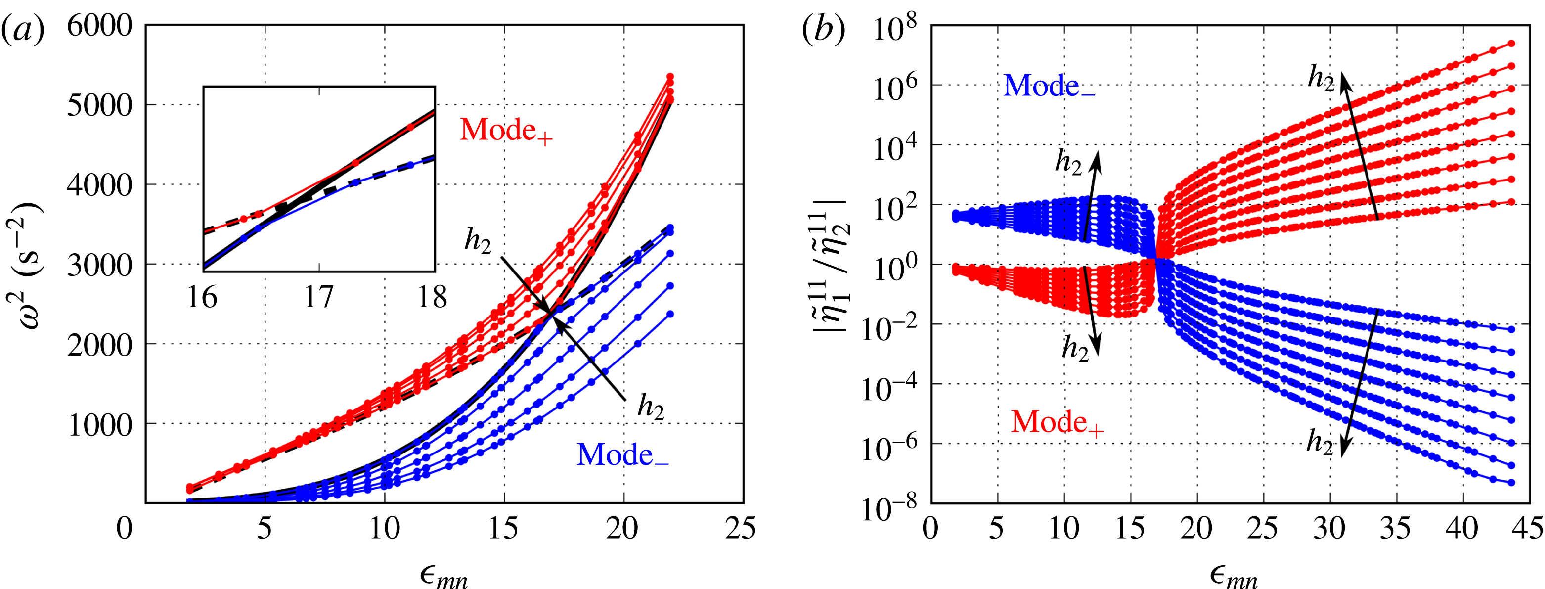
(a) Three-layer dispersion relations due to (2.21) and two-layer dispersion relations due to (2.24a
) and (2.24b
) of the
 $\text{Mg}\Vert \text{Sb}$
cell (table 1) for different salt-layer heights
 $h_{2}=0.15,0.2,0.3,0.5$
and
 $5\,\text{ cm}$
. The plus mode
 $\unicode[STIX]{x1D714}_{+}$
is red and the minus mode
 $\unicode[STIX]{x1D714}_{-}$
blue coloured. The solid black line shows the two-layer frequency of the upper interface
 $\unicode[STIX]{x1D702}_{1}$
and the dashed black line the two-layer frequency of the lower interface
 $\unicode[STIX]{x1D702}_{2}$
both for
 $h_{2}=5\,\text{ cm}$
. (b) Absolute value of the amplitude ratios due to (2.22) in dependence on
 $\unicode[STIX]{x1D716}_{mn}$
for
 $h_{2}=0.1,1.1,2.2,3.1,4.1,5.1,6.1$
and
 $7.1\,\text{ cm}$
.

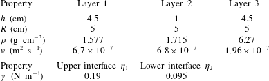
Cell parameters of the
 $\text{Mg}\Vert \text{Sb}$
cell from Weber et al. (Reference Weber, Beckstein, Herreman, Horstmann, Nore, Stefani and Weier2017b
) used to calculate the wave frequencies and amplitude ratios of figure 4.

In the first instance, to give the reader a better understanding, figure 4 shows exemplarily the frequencies (a) due to (2.21) as well as the amplitude ratios (b) due to (2.22). Both are given for varying electrolyte-layer heights in dependency of the wavenumber
 $\unicode[STIX]{x1D716}_{mn}$
for the same
 $\text{Mg}\Vert \text{Sb}$
cell numerically investigated by Weber et al. (Reference Weber, Beckstein, Herreman, Horstmann, Nore, Stefani and Weier2017b
). The cell parameters and material properties used are shown in table 1. Figure 4(a) clarifies that both frequency modes are progressively approaching the two-layer limits for increasing salt-layer heights. Another remarkable feature is the frequency transition appearing at
 $\unicode[STIX]{x1D716}_{mn}\approx 17$
, where the two-layer frequencies are crossing each other. The transition is emphasized in the zoomed window of figure 4(a) showing the two-layer frequencies
 $\unicode[STIX]{x1D714}_{\unicode[STIX]{x1D702}_{1}}$
and
 $\unicode[STIX]{x1D714}_{\unicode[STIX]{x1D702}_{2}}$
as well as the decoupled three-layer frequencies
 $\unicode[STIX]{x1D714}_{+}$
and
 $\unicode[STIX]{x1D714}_{-}$
for large salt layers. It can be seen that for small wavenumbers the fast mode
 $\unicode[STIX]{x1D714}_{+}$
is following the two-layer eigenfrequency
 $\unicode[STIX]{x1D714}_{\unicode[STIX]{x1D702}_{2}}$
of the lower interface while the slow mode
 $\unicode[STIX]{x1D714}_{-}$
oscillates with the two-layer frequency
 $\unicode[STIX]{x1D714}_{\unicode[STIX]{x1D702}_{1}}$
of the upper interface. From
 $\unicode[STIX]{x1D716}_{mn}\approx 17$
onwards both modes behave in precisely the opposite manner. Hence, both modes cannot be uniquely assigned to the natural frequencies of uncoupled interfaces. Such a behaviour has not been observed yet in coupled internal and surface waves (Issenmann et al.
Reference Issenmann, Laroche and Falcon2016) and leads to some new physical properties. Figure 4(b) shows the absolute values of the amplitude ratio clarifying the strength of coupling in dependence on
 $\unicode[STIX]{x1D716}_{mn}$
and
 $h_{2}$
. If we for instance focus on the smallest wavenumber
 $\unicode[STIX]{x1D716}_{11}$
representing the metal pad roll, one can see that for the
 $\text{Mg}\Vert \text{Sb}$
cell the amplitude ratios of both modes are not symmetric around
 $|\tilde{\unicode[STIX]{x1D702}}_{1}^{11}/\tilde{\unicode[STIX]{x1D702}}_{2}^{11}|=1$
. In this case, oscillations of the upper interface will influence the lower one only very slightly. The slow mode
 $\unicode[STIX]{x1D714}_{-}$
will be excited at the upper interface since it is close to its eigenfrequency. Further, the amplitude ratio is very large with
 $|\tilde{\unicode[STIX]{x1D702}}_{1}^{11}/\tilde{\unicode[STIX]{x1D702}}_{2}^{11}|_{-}\approx 38$
such that
 $\tilde{\unicode[STIX]{x1D702}}_{2}^{11}$
becomes negligibly small for reasonable values of
 $\tilde{\unicode[STIX]{x1D702}}_{1}^{11}$
. In contrast, perturbations of the lower interface with an eigenfrequency close to
 $\unicode[STIX]{x1D714}_{+}$
will substantially affect the upper one because there the amplitudes are strongly coupled
 $|\tilde{\unicode[STIX]{x1D702}}_{1}^{11}/\tilde{\unicode[STIX]{x1D702}}_{2}^{11}|_{+}\approx 0.7$
. The above mentioned transition can be seen as well in the amplitude ratio curves at
 $\unicode[STIX]{x1D716}_{mn}\approx 17$
. There, all curves intersect with
 $|\tilde{\unicode[STIX]{x1D702}}_{1}^{mn}/\tilde{\unicode[STIX]{x1D702}}_{2}^{mn}|_{\pm }\approx 1$
and both waves are perfectly coupled by both modes. That clarifies that there is not only an exchange of the frequencies, but also of the modes within the interfaces.
Equations (2.21) together with (2.22) are principally sufficient to completely describe the gravitational–capillary coupling dynamics. However, it is worthwhile also to analytically predict the intersection point and to understand the physical nature of this transition. While the presented transition as a function of the wavenumber is not of practical importance for LMBs, we have observed this transition also in dependence on many further cell parameters significantly changing for the various possible liquid metal and electrolyte combinations. We discovered that the influence of all cell parameters can be unified by only two dimensionless parameters. We can prove that by eliminating the frequencies in (2.19a ) and (2.19b ). This leads to a quadratic equation for the amplitude ratio:
 $$\begin{eqnarray}\displaystyle \left.\begin{array}{@{}l@{}}a\left({\displaystyle \frac{\tilde{\unicode[STIX]{x1D702}}_{1}^{mn}}{\tilde{\unicode[STIX]{x1D702}}_{2}^{mn}}}\right)^{2}+b{\displaystyle \frac{\tilde{\unicode[STIX]{x1D702}}_{1}^{mn}}{\tilde{\unicode[STIX]{x1D702}}_{2}^{mn}}}-c=0,\quad \text{with}\\ a={\displaystyle \frac{\unicode[STIX]{x1D70C}_{2}}{\sinh \left({\displaystyle \frac{\unicode[STIX]{x1D716}_{mn}}{R}}h_{2}\right)\left(\unicode[STIX]{x1D70C}_{1}\coth \left({\displaystyle \frac{\unicode[STIX]{x1D716}_{mn}}{R}}h_{1}\right)+\unicode[STIX]{x1D70C}_{2}\coth \left({\displaystyle \frac{\unicode[STIX]{x1D716}_{mn}}{R}}h_{2}\right)\right)}},\\ b=\left({\displaystyle \frac{(\unicode[STIX]{x1D70C}_{3}-\unicode[STIX]{x1D70C}_{2})g{\displaystyle \frac{\unicode[STIX]{x1D716}_{mn}}{R}}+\unicode[STIX]{x1D6FE}_{\unicode[STIX]{x1D702}_{2}}\left({\displaystyle \frac{\unicode[STIX]{x1D716}_{mn}}{R}}\right)^{3}}{(\unicode[STIX]{x1D70C}_{2}-\unicode[STIX]{x1D70C}_{1})g{\displaystyle \frac{\unicode[STIX]{x1D716}_{mn}}{R}}+\unicode[STIX]{x1D6FE}_{\unicode[STIX]{x1D702}_{1}}\left({\displaystyle \frac{\unicode[STIX]{x1D716}_{mn}}{R}}\right)^{3}}}-{\displaystyle \frac{\unicode[STIX]{x1D70C}_{2}\coth \left({\displaystyle \frac{\unicode[STIX]{x1D716}_{mn}}{R}}h_{2}\right)+\unicode[STIX]{x1D70C}_{3}\coth \left({\displaystyle \frac{\unicode[STIX]{x1D716}_{mn}}{R}}h_{3}\right)}{\unicode[STIX]{x1D70C}_{1}\coth \left({\displaystyle \frac{\unicode[STIX]{x1D716}_{mn}}{R}}h_{1}\right)+\unicode[STIX]{x1D70C}_{2}\coth \left({\displaystyle \frac{\unicode[STIX]{x1D716}_{mn}}{R}}h_{2}\right)}}\right),\\ c={\displaystyle \frac{\unicode[STIX]{x1D70C}_{2}}{\sinh \left({\displaystyle \frac{\unicode[STIX]{x1D716}_{mn}}{R}}h_{2}\right)\left(\unicode[STIX]{x1D70C}_{1}\coth \left({\displaystyle \frac{\unicode[STIX]{x1D716}_{mn}}{R}}h_{1}\right)+\unicode[STIX]{x1D70C}_{2}\coth \left({\displaystyle \frac{\unicode[STIX]{x1D716}_{mn}}{R}}h_{2}\right)\right)}}\\ \qquad \times {\displaystyle \frac{(\unicode[STIX]{x1D70C}_{3}-\unicode[STIX]{x1D70C}_{2})g{\displaystyle \frac{\unicode[STIX]{x1D716}_{mn}}{R}}+\unicode[STIX]{x1D6FE}_{\unicode[STIX]{x1D702}_{2}}\left({\displaystyle \frac{\unicode[STIX]{x1D716}_{mn}}{R}}\right)^{3}}{(\unicode[STIX]{x1D70C}_{2}-\unicode[STIX]{x1D70C}_{1})g{\displaystyle \frac{\unicode[STIX]{x1D716}_{mn}}{R}}+\unicode[STIX]{x1D6FE}_{\unicode[STIX]{x1D702}_{1}}\left({\displaystyle \frac{\unicode[STIX]{x1D716}_{mn}}{R}}\right)^{3}}}.\end{array}\right\}\qquad & & \displaystyle\end{eqnarray}$$
As clarified in figure 4(b), the transition always appears at the intersection point of the modes, where the absolute values of the amplitude ratios have to equalize
 $$\begin{eqnarray}\left|{\displaystyle \frac{\tilde{\unicode[STIX]{x1D702}}_{1}^{mn}}{\tilde{\unicode[STIX]{x1D702}}_{2}^{mn}}}\right|_{+}\stackrel{!}{=}\left|{\displaystyle \frac{\tilde{\unicode[STIX]{x1D702}}_{1}^{mn}}{\tilde{\unicode[STIX]{x1D702}}_{2}^{mn}}}\right|_{-}.\end{eqnarray}$$
That is automatically fulfilled if (2.27) has only one solution, which in turn is guaranteed only if
 $b$
vanishes. This is again fulfilled only for
 $$\begin{eqnarray}{\mathcal{A}}\stackrel{!}{=}{\mathcal{B}},\end{eqnarray}$$
where the two dimensionless numbers
 ${\mathcal{A}}$
and
 ${\mathcal{B}}$
are defined with
 $$\begin{eqnarray}\displaystyle & \displaystyle {\mathcal{A}}:={\displaystyle \frac{(\unicode[STIX]{x1D70C}_{3}-\unicode[STIX]{x1D70C}_{2})gR^{2}+\unicode[STIX]{x1D6FE}_{\unicode[STIX]{x1D702}_{2}}\unicode[STIX]{x1D716}_{mn}^{2}}{(\unicode[STIX]{x1D70C}_{2}-\unicode[STIX]{x1D70C}_{1})gR^{2}+\unicode[STIX]{x1D6FE}_{\unicode[STIX]{x1D702}_{1}}\unicode[STIX]{x1D716}_{mn}^{2}}}, & \displaystyle\end{eqnarray}$$
 $$\begin{eqnarray}\displaystyle & \displaystyle {\mathcal{B}}:={\displaystyle \frac{\unicode[STIX]{x1D70C}_{2}\coth \left({\displaystyle \frac{\unicode[STIX]{x1D716}_{mn}}{R}}h_{2}\right)+\unicode[STIX]{x1D70C}_{3}\coth \left({\displaystyle \frac{\unicode[STIX]{x1D716}_{mn}}{R}}h_{3}\right)}{\unicode[STIX]{x1D70C}_{1}\coth \left({\displaystyle \frac{\unicode[STIX]{x1D716}_{mn}}{R}}h_{1}\right)+\unicode[STIX]{x1D70C}_{2}\coth \left({\displaystyle \frac{\unicode[STIX]{x1D716}_{mn}}{R}}h_{2}\right)}}. & \displaystyle\end{eqnarray}$$
Hence, the parameters
 ${\mathcal{A}}$
and
 ${\mathcal{B}}$
completely determine the transition.
 ${\mathcal{A}}$
may be interpreted as the ratio of the restoring gravity and capillary forces acting on both waves, whereas
 ${\mathcal{B}}$
describes the inertia distribution in the battery system. However, it can be shown that in practical cases the transition process is mainly captured by
 ${\mathcal{A}}$
alone. For the desired thin electrolyte-layer limit
 $h_{2}\rightarrow 0$
,
 ${\mathcal{B}}$
converges asymptotically to 1 and (2.27) simplifies to
 $$\begin{eqnarray}\left({\displaystyle \frac{\tilde{\unicode[STIX]{x1D702}}_{1}^{mn}}{\tilde{\unicode[STIX]{x1D702}}_{2}^{mn}}}\right)^{2}+({\mathcal{A}}-1){\displaystyle \frac{\tilde{\unicode[STIX]{x1D702}}_{1}^{mn}}{\tilde{\unicode[STIX]{x1D702}}_{2}^{mn}}}-{\mathcal{A}}=0.\end{eqnarray}$$
In this limit the amplitude ratio has become independent of
 ${\mathcal{B}}$
and offers two analytical solutions
 $$\begin{eqnarray}{\displaystyle \frac{\tilde{\unicode[STIX]{x1D702}}_{1}^{mn}}{\tilde{\unicode[STIX]{x1D702}}_{2}^{mn}}}_{+}=1\quad \text{and}\quad {\displaystyle \frac{\tilde{\unicode[STIX]{x1D702}}_{1}^{mn}}{\tilde{\unicode[STIX]{x1D702}}_{2}^{mn}}}_{-}=-{\mathcal{A}}.\end{eqnarray}$$
From this we note that for thin salt layers the interfaces are perfectly coupled for all parameters when they are excited by the fast mode
 $\unicode[STIX]{x1D714}_{+}$
. In contrast, the amplitude ratio of the slow mode
 $\unicode[STIX]{x1D714}_{-}$
is directly determined by
 ${\mathcal{A}}$
.
Finally,
 ${\mathcal{A}}$
and
 ${\mathcal{B}}$
can be further exploited to physically understand the mode transition. At first we consider the limits of pure gravity and pure capillary waves. In these limits,
 ${\mathcal{A}}$
simplifies to
 $$\begin{eqnarray}{\mathcal{A}}_{gravity}={\displaystyle \frac{\unicode[STIX]{x1D70C}_{3}-\unicode[STIX]{x1D70C}_{2}}{\unicode[STIX]{x1D70C}_{2}-\unicode[STIX]{x1D70C}_{1}}}\quad \text{or}\quad {\mathcal{A}}_{capillary}={\displaystyle \frac{\unicode[STIX]{x1D6FE}_{\unicode[STIX]{x1D702}_{2}}}{\unicode[STIX]{x1D6FE}_{\unicode[STIX]{x1D702}_{1}}}},\end{eqnarray}$$
respectively. Hence, in large-scale LMBs the wave coupling is determined only by the ratio of the density differences.
 ${\mathcal{A}}_{gravity}$
is the most important control parameter that should always be considered for predicting resonance. Further, the wavenumber-dependent mode transition, as shown in figure 4, can be explained considering both limits: for the
 $\text{Mg}\Vert \text{Sb}$
cell we find
 ${\mathcal{A}}_{gravity}>1$
but
 ${\mathcal{A}}_{capillary}<1$
. Consequently, this mode transition arose due to the change from gravity to capillary waves turning the sign of
 ${\mathcal{A}}$
.
The coupling mechanism can be further understood by noting that
 ${\mathcal{A}}/{\mathcal{B}}$
can be expressed by the ratio of the two-layer frequencies
 $$\begin{eqnarray}{\displaystyle \frac{{\mathcal{A}}}{{\mathcal{B}}}}={\displaystyle \frac{\unicode[STIX]{x1D714}_{\unicode[STIX]{x1D702}_{2}}^{2}}{\unicode[STIX]{x1D714}_{\unicode[STIX]{x1D702}_{1}}^{2}}}.\end{eqnarray}$$
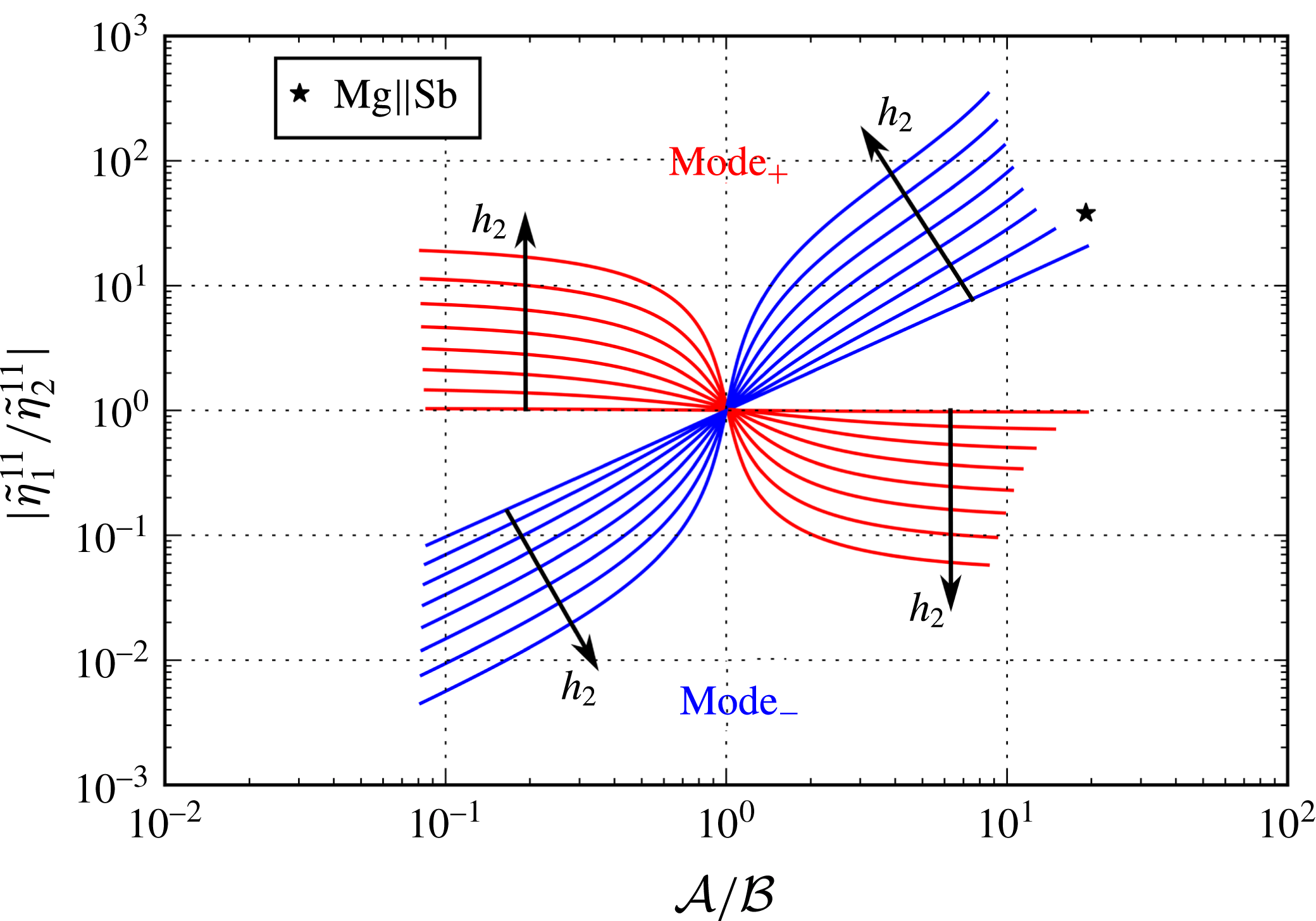
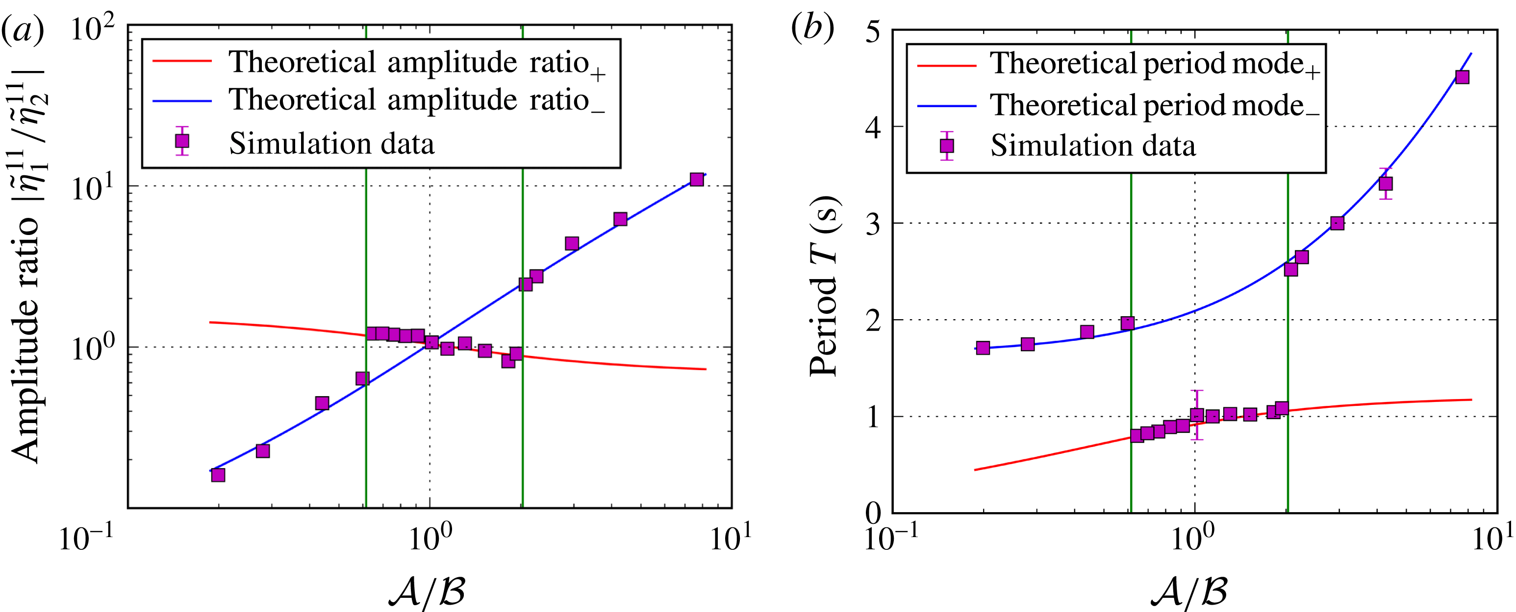
Absolute values of the amplitude ratios due to (2.22) for the metal pad roll mode
 $\unicode[STIX]{x1D716}_{11}$
in dependence on
 ${\mathcal{A}}/{\mathcal{B}}$
with varying salt-layer thicknesses
 $h_{2}=0.1,1,2,3,4,5,6$
and
 $7~\text{cm}$
exemplarily plotted using the generic
 $\text{Mg}\Vert \text{Sb}$
cell parameters from Weber et al. (Reference Weber, Beckstein, Herreman, Horstmann, Nore, Stefani and Weier2017b
) (table 1). To diversify
 ${\mathcal{A}}$
and
 ${\mathcal{B}}$
,
 $\unicode[STIX]{x1D70C}_{3}$
was changed from
 $1716$
up to
 $5000~\text{kg}~\text{m}^{-3}$
.

Thus, as one would intuitively expect, the highest coupling indeed arises where the two-layer eigenfrequencies coincide and the interfaces step into resonance. The ratio
 ${\mathcal{A}}/{\mathcal{B}}$
quantifies the difference of the natural frequencies of both interfaces and therefore determines the strength of the coupling. For the important thin salt-layer limit
 $h_{2}\rightarrow 0$
, we further obtain
 $$\begin{eqnarray}\left|{\displaystyle \frac{\tilde{\unicode[STIX]{x1D702}}_{1}^{mn}}{\tilde{\unicode[STIX]{x1D702}}_{2}^{mn}}}\right|_{-}={\mathcal{A}}={\displaystyle \frac{\unicode[STIX]{x1D714}_{\unicode[STIX]{x1D702}_{2}}^{2}}{\unicode[STIX]{x1D714}_{\unicode[STIX]{x1D702}_{1}}^{2}}},\end{eqnarray}$$
showing that the amplitude ratio corresponding to the slow mode
 $\unicode[STIX]{x1D714}_{-}$
is directly determined by the ratio of the two-layer frequencies.
All these results are exemplified in figure 5 showing the absolute values of the amplitude ratios in dependence on
 ${\mathcal{A}}/{\mathcal{B}}$
for different salt-layer thicknesses of the
 $\text{Mg}\Vert \text{Sb}$
cell. All curves are indeed crossing at
 ${\mathcal{A}}={\mathcal{B}}$
. The two inner lines for the smallest chosen
 $h_{2}$
correspond to the solutions (2.33) bounding the maximum coupling state. For large
 ${\mathcal{A}}/{\mathcal{B}}\gg 1$
the antisymmetric mode
 $\unicode[STIX]{x1D714}_{-}$
dominates in the upper interface
 $\unicode[STIX]{x1D702}_{1}$
, while for low values
 ${\mathcal{A}}/{\mathcal{B}}\ll 1$
this mode is more prominent in the lower one
 $\unicode[STIX]{x1D702}_{2}$
. The coupling state of the symmetric mode
 $\unicode[STIX]{x1D714}_{+}$
in contrast is not limited by
 ${\mathcal{A}}/{\mathcal{B}}$
since for sufficiently small
 $h_{2}$
the interfaces are always perfectly coupled by that mode.
2.4 Coupling criterion for LMBs
These findings now can be exploited to determine for which parameter regimes coupled dynamics must be considered and in which cases two-layer stability analysis, as practiced e.g. in the context of ARCs, is sufficient to understand interfacial instabilities in LMBs. At first it is desirable to predict which coupling mode will be excited by the arising Lorentz forces. As presented in the introduction, in two-layer systems the MPRI can be appropriately described by the Sele criterion. Since interfacial tension was respected for the coupling theory, it also has to be included into the Sele criterion. Following Gerbeau et al. (Reference Gerbeau, Le Bris and Lelièvre2006),
 $\unicode[STIX]{x1D6FD}$
can be regarded as the ratio of the electromagnetic force due to interface displacements to the gravity force exerted on the interface due to the same displacements. By considering the sum of gravity and capillarity as the acting restoring force, we get modified Sele criteria for both interfaces
 $$\begin{eqnarray}\displaystyle & \displaystyle \unicode[STIX]{x1D6FD}_{\unicode[STIX]{x1D702}_{1}}={\displaystyle \frac{I_{0}b_{z}}{\left[(\unicode[STIX]{x1D70C}_{2}-\unicode[STIX]{x1D70C}_{1})g+\unicode[STIX]{x1D6FE}_{\unicode[STIX]{x1D702}_{1}}\left({\displaystyle \frac{\unicode[STIX]{x1D716}_{11}}{R}}\right)^{2}\right]h_{1}h_{2}}}>\unicode[STIX]{x1D6FD}_{crit}, & \displaystyle\end{eqnarray}$$
 $$\begin{eqnarray}\displaystyle & \displaystyle \unicode[STIX]{x1D6FD}_{\unicode[STIX]{x1D702}_{2}}={\displaystyle \frac{I_{0}b_{z}}{\left[(\unicode[STIX]{x1D70C}_{3}-\unicode[STIX]{x1D70C}_{2})g+\unicode[STIX]{x1D6FE}_{\unicode[STIX]{x1D702}_{2}}\left({\displaystyle \frac{\unicode[STIX]{x1D716}_{11}}{R}}\right)^{2}\right]h_{2}h_{3}}}>\unicode[STIX]{x1D6FD}_{crit}. & \displaystyle\end{eqnarray}$$
From these criteria we can easily identify which interface is becoming unstable first. For example, for large-size LMBs it is always the interface with the lower density difference. The ratio
 $\unicode[STIX]{x1D6FD}_{\unicode[STIX]{x1D702}_{2}}/\unicode[STIX]{x1D6FD}_{\unicode[STIX]{x1D702}_{1}}$
can be directly expressed in dependence of
 ${\mathcal{A}}$
 $$\begin{eqnarray}{\displaystyle \frac{\unicode[STIX]{x1D6FD}_{\unicode[STIX]{x1D702}_{2}}}{\unicode[STIX]{x1D6FD}_{\unicode[STIX]{x1D702}_{1}}}}={\displaystyle \frac{((\unicode[STIX]{x1D70C}_{2}-\unicode[STIX]{x1D70C}_{1})gR^{2}+\unicode[STIX]{x1D6FE}_{\unicode[STIX]{x1D702}_{1}}\unicode[STIX]{x1D716}_{11}^{2})h_{1}}{((\unicode[STIX]{x1D70C}_{3}-\unicode[STIX]{x1D70C}_{2})gR^{2}+\unicode[STIX]{x1D6FE}_{\unicode[STIX]{x1D702}_{2}}\unicode[STIX]{x1D716}_{11}^{2})h_{3}}}={\displaystyle \frac{1}{{\mathcal{A}}}}{\displaystyle \frac{h_{1}}{h_{3}}}\end{eqnarray}$$
showing that for large
 ${\mathcal{A}}$
the upper interface will be more unstable while for small
 ${\mathcal{A}}$
the lower interface becomes more susceptible to electromagnetic excitation. By considering that at the first moment the natural two-layer frequencies will be excited until the third layer is interacting after some response time, it can be clarified that only the slow mode
 $\unicode[STIX]{x1D714}_{-}$
will be excited in LMBs for small and large values of
 ${\mathcal{A}}$
because for large
 ${\mathcal{A}}$
the natural two-layer frequency of the first excited upper interface is slower and close to
 $\unicode[STIX]{x1D714}_{-}$
(see (2.19) or figure 4
a) while for small
 ${\mathcal{A}}$
the lower interface becomes slower and even close to
 $\unicode[STIX]{x1D714}_{-}$
. In both cases only the antisymmetric mode
 $\unicode[STIX]{x1D714}_{-}$
develops such that LMBs can principally decouple. On that basis a coupling criterion can be deduced. Note, that for the limit
 $h_{2}\rightarrow 0$
the coupling is always on its highest level. When neglecting
 $\unicode[STIX]{x1D714}_{+}$
, we find from (2.33) that
 $$\begin{eqnarray}\left|{\displaystyle \frac{\tilde{\unicode[STIX]{x1D702}}_{1}^{mn}}{\tilde{\unicode[STIX]{x1D702}}_{2}^{mn}}}\right|\geqslant {\mathcal{A}}\quad \text{for }{\mathcal{A}}\gg 1\quad \text{and}\quad \left|{\displaystyle \frac{\tilde{\unicode[STIX]{x1D702}}_{1}^{mn}}{\tilde{\unicode[STIX]{x1D702}}_{2}^{mn}}}\right|\leqslant {\mathcal{A}}\quad \text{for }{\mathcal{A}}\ll 1.\end{eqnarray}$$
By defining a decoupling threshold such that the interfaces are assumed to be decoupled for
 $|\tilde{\unicode[STIX]{x1D702}}_{1}^{mn}/\tilde{\unicode[STIX]{x1D702}}_{2}^{mn}|>\unicode[STIX]{x1D712}$
or
 $|\tilde{\unicode[STIX]{x1D702}}_{1}^{mn}/\tilde{\unicode[STIX]{x1D702}}_{2}^{mn}|<1/\unicode[STIX]{x1D712}$
, we suggest the following criterion to evaluate the importance of wave coupling in LMBs:
 $$\begin{eqnarray}\displaystyle & & \displaystyle \unicode[STIX]{x1D702}_{2}\approx 0\quad \text{ if}\left\{\begin{array}{@{}ll@{}}{\mathcal{A}}>\unicode[STIX]{x1D712}{\displaystyle \frac{h_{3}}{h_{1}}} & \text{for }h_{3}\geqslant h_{1}\\ {\mathcal{A}}>\unicode[STIX]{x1D712} & \text{for }h_{3}<h_{1},\end{array}\right.\end{eqnarray}$$
 $$\begin{eqnarray}\displaystyle & & \displaystyle \unicode[STIX]{x1D702}_{1}\approx 0\text{ if}\left\{\begin{array}{@{}ll@{}}{\mathcal{A}}<{\displaystyle \frac{1}{\unicode[STIX]{x1D712}}}{\displaystyle \frac{h_{3}}{h_{1}}} & \text{for }h_{3}\leqslant h_{1}\\ {\mathcal{A}}<{\displaystyle \frac{1}{\unicode[STIX]{x1D712}}} & \text{for }h_{3}>h_{1}.\end{array}\right.\end{eqnarray}$$
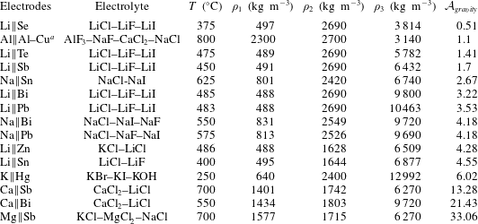
Coupling parameter
 ${\mathcal{A}}_{gravity}$
calculated for different possible working material combinations. The densities are reported at working temperature
 $T$
, see Lyon (Reference Lyon1954), Agruss, Karas & Decker (Reference Agruss, Karas and Decker1962), Weaver, Smith & Willmann (Reference Weaver, Smith and Willmann1962), Karas & Mangus (Reference Karas and Mangus1963), Cairns et al. (Reference Cairns, Crouthamel, Fischer, Foster, Hesson, Johnson, Shimotake and Tevebaugh1967), Herédy et al. (Reference Herédy, Iverson, Ulrich and Recht1967), Cairns & Shimotake (Reference Cairns and Shimotake1969a
,Reference Cairns and Shimotake
b
), Shimotake, Rogers & Cairns (Reference Shimotake, Rogers and Cairns1969), Swinkels (Reference Swinkels, Braunstein, Mamantov and Smith1971), Janz et al. (Reference Janz, Tomkins, Allen, Downey, Gardner, Krebs and Singer1975, Reference Janz, Allen, Bansal, Murphy and Tomkins1979), Chum & Osteryoung (Reference Chum and Osteryoung1980, Reference Chum and Osteryoung1981), Zinkle (Reference Zinkle1998), Smithells, Gale & Totemeier (Reference Smithells, Gale and Totemeier2004), Sobolev (Reference Sobolev2007), International Atomic Energy Agency (2008), Sobolev (Reference Sobolev2010), Aqra & Ayyad (Reference Aqra and Ayyad2011), Bradwell (Reference Bradwell2011), Bradwell et al. (Reference Bradwell, Kim, Sirk and Sadoway2012), Spatocco, Burke & Sadoway (Reference Spatocco, Burke and Sadoway2014), Wang et al. (Reference Wang, Jiang, Chung, Ouchi, Burke, Boysen, Bradwell, Kim, Muecke and Sadoway2014).
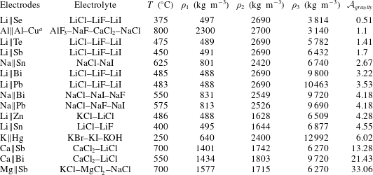
a Aluminium-refining cell (Pearson & Phillips Reference Pearson and Phillips1957)
These conditions guarantee both that only one interface is excited due to (2.39) and the amplitude ratio is becoming large or small enough due to (2.40).
 $\unicode[STIX]{x1D712}$
has to be chosen arbitrarily depending on the expediency. In the context of the metal pad roll dynamics we numerically found that
 $\unicode[STIX]{x1D712}=10$
is suitable as it will be discussed in the second part. In the case of the
 $\text{Mg}\Vert \text{Sb}$
battery numerically investigated with and without interfacial tension by Bojarevics & Tucs (Reference Bojarevics, Tucs and Ratvik2017) and Weber et al. (Reference Weber, Beckstein, Herreman, Horstmann, Nore, Stefani and Weier2017b
) we find high coupling parameters
 ${\mathcal{A}}\approx 28$
and
 ${\mathcal{A}}_{gravity}\approx 33$
both clearly exceeding the coupling threshold. Indeed, both studies obtained wave motion essentially in the upper interface propagating with the frequency of the slow mode
 $\unicode[STIX]{x1D714}_{-}$
. To determine the practical importance of wave coupling in large-size LMBs,
 ${\mathcal{A}}_{\text{gravity}}$
was calculated for further metals. Table 2 shows the densities at operation temperature and the corresponding coupling parameter
 ${\mathcal{A}}_{gravity}$
for most common metal and electrolyte combinations concerned as possible working materials for LMBs in the literature. It can be seen that the so far studied
 $\text{Mg}\Vert \text{Sb}$
cells coincidentally typifies the extreme case of lowest wave coupling. Most batteries reveal values of
 ${\mathcal{A}}_{gravity}$
between 3 and 6 where motion is present in both interfaces. Hence, coupling dynamics is indeed of high importance for most LMBs and may not be generally neglected as has previously been assumed on the basis of the obtained dynamics in
 $\text{Mg}\Vert \text{Sb}$
cells.
Interestingly, the density ratios in three-layer aluminium-refining cells are such that the interfaces in those cells are strongly coupled as well (see table 2). The following discussion applies therefore equally to aluminium-refining cells. However, the refining process – not limited by the open-circuit voltage – allows for much thicker electrolyte layers, typically between 8 and 25 cm (Beljajew, Rapoport & Firsanowa Reference Beljajew, Rapoport and Firsanowa1957; Pearson & Phillips Reference Pearson and Phillips1957).
3 Numerical study of coupled interfacial waves
All the above presented theoretical results and conclusions were derived only for inviscid gravity–capillary waves. All electromagnetic effects and the rotational part of the flow were neglected. Consequently, it is necessary to verify the applicability of the potential flow theory for more realistic electromagnetically driven battery systems involving also the rotational part of the flow. Further, from theory it is not evident which modes will evolve for strongly coupled interfaces at
 $A\approx 1$
where both eigenfrequencies can be excited simultaneously. For this purpose, we conducted multiphase DNS in the predicted coupled wave regime
 $0.1<{\mathcal{A}}<10$
taking into account the entire magnetohydrodynamics. We found three different coupling regimes with different stability properties. Besides the theoretically predicted antisymmetric motion for relatively small and large
 ${\mathcal{A}}$
, novel propagation dynamics was discovered for strongly coupled interfaces
 $0.7\lesssim {\mathcal{A}}\lesssim 2.1$
which will be presented in the following sections.
3.1 Numerical set-up and procedure
For the numerical study we used the three-dimensional multiphase DNS solver developed by Weber et al. (Reference Weber, Beckstein, Herreman, Horstmann, Nore, Stefani and Weier2017b ) particularly to investigate MHD instabilities in multilayer systems. The solver is implemented in the open source computational fluid dynamics (CFD) library OpenFOAM. The physical model is sketched in appendix B, further detailed information can be found in Weber et al. (Reference Weber, Beckstein, Galindo, Herreman, Nore, Stefani and Weier2017a ,Reference Weber, Beckstein, Herreman, Horstmann, Nore, Stefani and Weier b ).
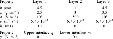
Used generic simulation parameters of the standard case yielding
 ${\mathcal{A}}=1$
.

On the basis of the theoretical results a parameter study around
 ${\mathcal{A}}=1$
was performed to investigate strongly coupled wave dynamics. To reach
 ${\mathcal{A}}=1$
, a generic standard case of equal metal-layer heights
 $h_{i}$
, conductivities
 $\unicode[STIX]{x1D70E}_{i}$
, density differences
 $\unicode[STIX]{x0394}\unicode[STIX]{x1D70C}$
, interfacial tensions
 $\unicode[STIX]{x1D6FE}_{\unicode[STIX]{x1D702}_{1}}$
and
 $\unicode[STIX]{x1D6FE}_{\unicode[STIX]{x1D702}_{2}}$
as well as viscosities
 $\unicode[STIX]{x1D708}_{i}$
was defined. The parameters used are shown in table 3. Because of the small height chosen for the electrolyte, the influence of
 ${\mathcal{B}}$
is very weak such that it is sufficient to describe the coupling only by
 ${\mathcal{A}}$
. In order to capture also non-shallow water dynamics, all simulations were conducted in a aspect-ratio-one cylindrical tank of equal diameter
 $D$
and height
 $H$
of
 $10~\text{cm}$
. The grid was constructed of purely orthogonal hexaedra with a lateral resolution of 50 cells and an axial resolution of 60 cells. This resolution was found to be sufficient to capture long-wave instabilities by employing a grid refinement study. The results did not significantly change when using finer grids.
Various simulation series were conducted for different values of
 ${\mathcal{A}}$
.
 ${\mathcal{A}}$
was modified stepwise by adapting only the density of the upper layer
 $\unicode[STIX]{x1D70C}_{1}$
. As predicted by the theory, we achieved the same results by modifying other
 ${\mathcal{A}}$
-dependent parameters. Simulations with different cell currents
 $I_{0}$
were performed to find the stability onsets by successively increasing
 $I_{0}$
. Once the current becomes large enough (
 $I_{0}>I_{c}$
) to destabilize the system, small numerical errors will grow and form the metal pad roll after a while. After first noticeable interfacial displacements were identified for
 $I_{0}>I_{c}$
, we ensured to leave the system sufficient time to reach a steady wave propagation state or to develop a short-circuit. Sufficient means here that we only accepted wave propagation as converged if both, the interface amplitudes and the mean velocity in the cell, were found to be constant for at least 30 periods. By that procedure the propagation regime between the rest state and the short-circuit was identified for all investigated
 ${\mathcal{A}}$
in dependence on the cell current. Finally, exemplary simulations in the propagation regime were chosen to evaluate the wave frequencies and amplitude ratios. It was ensured that the amplitudes were sufficiently small to allow comparison with linear wave theory.
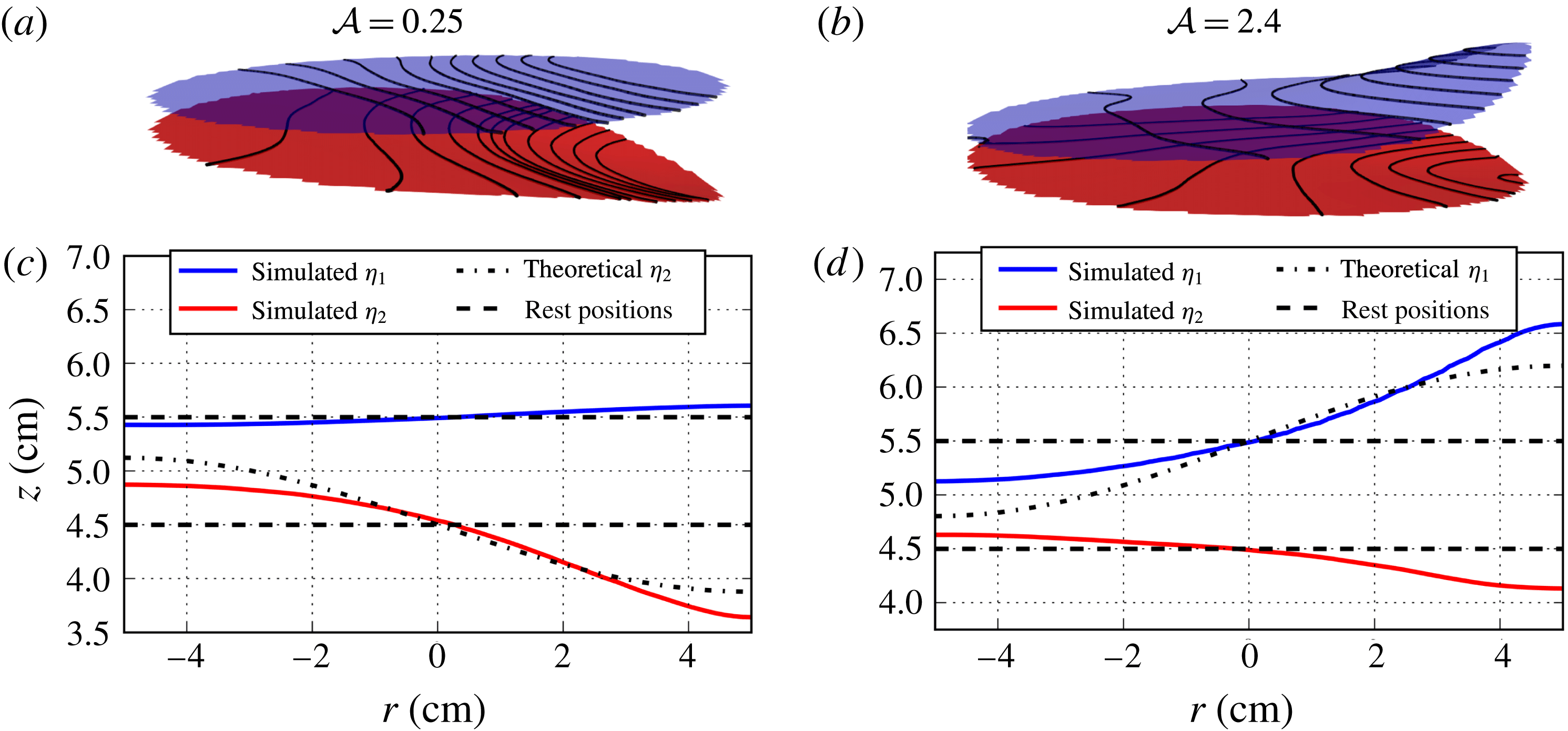
Exemplary contour plots of the excited interfaces for coupling parameters
 ${\mathcal{A}}=0.25$
(a) and
 ${\mathcal{A}}=2.4$
(b). (c,d
) Cross-sections of the corresponding interface contours
 $\unicode[STIX]{x1D702}_{1}$
(blue) and
 $\unicode[STIX]{x1D702}_{2}$
(red) in the
 $r$
–
 $z$
planes orientated along the highest amplitude shaping. In addition, the dashed lines mark the rest position of the interfaces and the dotted lines show the radial component of the theoretical gravity–capillary modes due to (2.12a
) and (2.12b
).

3.2 Numerical results
For all investigated coupling parameters interfacial motion could be confirmed in accordance with the theoretical predictions. In general, we found two distinguishable coupling regimes in dependence on
 ${\mathcal{A}}$
comprising fundamentally different coupling dynamics. The first regime was found for
 $0.7\lesssim {\mathcal{A}}\lesssim 2$
, where the amplitudes of both interfaces are similarly strong. This regime involves complex dynamics and various possible wave modes that can evolve. We call it from now on the ‘strongly coupled regime’. Respectively, for
 ${\mathcal{A}}\lesssim 0.7$
and
 ${\mathcal{A}}\gtrsim 2$
a second regime, later on referred to as the ‘weakly coupled regime’, was found, where always one interface was dominant. In these simulations we indeed obtained only the antisymmetric coupling
 $\unicode[STIX]{x1D714}_{-}$
as predicted by the theory. At first, characteristic modes observed for both regimes are introduced qualitatively in the following section. For reasons of clarity, the weakly coupled regime is presented first.
3.2.1 Weakly coupled regime
First of all the obtained interfacial shapes and directions of rotation are qualitatively analysed. Figures 6(a) and 6(b) show the contours of both interfaces for the exemplarily chosen values
 ${\mathcal{A}}=0.25$
and
 ${\mathcal{A}}=2.4$
, respectively. It can be seen that in both cases the interfaces are antisymmetrically displaced. For
 ${\mathcal{A}}=0.25$
the lower interface is more strongly deformed, where for
 ${\mathcal{A}}=2.4$
the upper interface deflects more. The resulting amplitude ratios can be identified more clearly in figure 6(c,d), showing cross-sections of the interface contours in the
 $r$
–
 $z$
planes orientated along the highest amplitude shaping. It becomes apparent that the amplitude of the subordinate upper interface for
 ${\mathcal{A}}=0.25$
is significantly smaller than the amplitude of the subordinate lower interface for
 ${\mathcal{A}}=2.4$
. That is in qualitative agreement with the theoretical slow mode amplitude ratios yielding disparate values of
 $|\tilde{\unicode[STIX]{x1D702}}_{1}^{mn}/\tilde{\unicode[STIX]{x1D702}}_{2}^{mn}|_{-}=0.18$
and
 $|\tilde{\unicode[STIX]{x1D702}}_{1}^{mn}/\tilde{\unicode[STIX]{x1D702}}_{2}^{mn}|_{-}=2.8$
. In addition, figure 6(c,d) further shows the theoretical radial shape due to (2.12a
) and (2.12b
) of the superordinate interfaces. Clear deviations between the numerical and analytical gravitational solutions can be recognized. In comparison to the gravitational modes, the magnetically driven interfacial waves are not symmetrically displaced around the rest positions. Rather, the interfaces tip away from each other such that the emergence of a short-circuit is counteracted. Hence, the theory tends here to overestimate the threat of short-circuits.
Further, for both exemplary cases different directions of rotations of the interfaces were observed. For
 ${\mathcal{A}}=0.25$
both interfaces rotate synchronously clockwise and for
 ${\mathcal{A}}=2.4$
counterclockwise. The same behaviour holds true for all investigated
 ${\mathcal{A}}\lesssim 0.7$
(clockwise) and
 ${\mathcal{A}}\gtrsim 2$
(counterclockwise). Hence, the direction of rotation in the weakly coupled regime is uniquely determined by
 ${\mathcal{A}}$
(and also
 ${\mathcal{B}}$
for unpractical high electrolyte layers) and the initial question from the introduction concerning the unknown rotation direction is clarified. This behaviour can be explained by the fact that the larger displaced interface, that is determined by
 ${\mathcal{A}}$
, causes higher horizontal compensation currents and thus a larger resulting Lorentz force than the smaller one. Since we know from the coupling analysis that both interfaces can only rotate synchronously in the same direction, the overall coupled rotation is determined by the Lorentz force associated with the larger displaced interface that overcompensates the oppositely directed Lorentz force caused by the small interface.
3.2.2 Strongly coupled regime
Exemplary contour plots of the excited interfaces for the coupling parameter
 ${\mathcal{A}}=0.9$
with the applied cell currents of
 $I=400~\text{A}$
(a) and
 $I=500~\text{A}$
(b). These currents lead to antisymmetric and symmetric wave coupling, respectively. (c,d
) Cross-sections of the corresponding interface contours
 $\unicode[STIX]{x1D702}_{1}$
(blue) and
 $\unicode[STIX]{x1D702}_{2}$
(red) in the
 $r$
–
 $z$
planes orientated along the highest amplitude shaping. (c) Shows in addition the fitted curves due to (4.3a
) and (4.3b
). (e,f
) Depict further the compensation current vectors in the same cross-section. A superimposed colour map highlights the radial (horizontal) component of the compensation currents.

For coupling parameters closer to one (
 $0.7\lesssim {\mathcal{A}}\lesssim 2$
) far more complex dynamics was observed. Note first that these regime thresholds are purely empirical at this stage. They may change in dependence on
 $h_{2}$
(affecting
 ${\mathcal{B}}$
) and possibly on further parameters not occurring in
 ${\mathcal{A}}$
and
 ${\mathcal{B}}$
like the viscosities and electrical conductivities. In this regime, we found different coupling modes and excited wavenumbers as well as a non-oscillatory instability in dependence on the cell current. Further, time-dependent mode transitions were found such that one mode can merge into another one spontaneously making analysis more complicated. However, two characteristic flow states were found that are mainly present in this regime exemplarily shown in figure 7. For relatively low applied cell currents slightly above the observed stability thresholds, we always found oppositely directed radial-symmetric rotating interfaces, as exemplarily shown in figure 7(a) and figure 7(c). This state largely differs from the MPRI in the physical sense since we observed that these vortex shapes can persist for minutes or even for the complete simulation depending on the cell currents. Hence, it can be considered as a quasi-steady non-oscillatory instability that cannot be described by the wall reflection of oscillating interfacial waves, compare to § 1. Figure 7(e) shows in addition the induced radial compensation currents in cross-section. In contrast to the metal pad roll mode, two closed current loops can be identified leading to pure azimuthal Lorentz forces inducing oppositely directed circular motions in the liquid electrodes. In § 4.1 we give a detailed explanation how centripetal pressure differences can cause this instability.
For higher applied cell currents, a second characteristic state was found to develop: symmetrically coupled in-phase rotating waves with the expected wavenumber
 $\unicode[STIX]{x1D716}_{11}$
associated with the metal pad roll, as depicted in figure 7(b,d). Also for high cell currents close to the short-circuit onset, the radial instability (figure 7
a) arose first. But for sufficiently high cell currents this coupling state always spontaneously turned into the symmetric mode (figure 7
b) after some time, then remained preserved, or – in only very few cases – once again turned into the previously presented antisymmetric mode of the weakly coupled regime (§ 3.2.1). This instability even strongly differs from the common MPRI mechanism. It seems to be counterintuitive at first glance since the metal pad is always explained by a redistribution of the cell currents due to changes of the electrical resistivity caused by electrolyte-layer deformations. But for parallel interfaces there is no preferred direction for the currents to choose because the salt-layer height remains constant everywhere. Thus, horizontal compensation currents are not expected to arise. However, it can be seen from figure 7(f) that here horizontal currents indeed appear in the electrolyte. This is in contrast to the common assumption stating that the current remains almost vertical in the low conductivity electrolyte. A detailed explanation unravelling that issue is given in § 4.2.
For the sake of completeness, it should be noted that besides the modes presented here we sometimes observed also higher modes or mode superpositions in particular for high cell currents near the short-circuit onset. However, these waves were only temporarily stable and seemed to appear randomly. All in all, the two modes presented here were highly dominant and can be considered as the characteristic modes of the strongly coupled regime. However, the mode dynamics was found to be far more complex and cannot be precisely predicted at this stage.
Interestingly, the observed transition from antisymmetrically coupled waves to symmetrically coupled waves was also numerically found recently by Zikanov (Reference Zikanov2017) in rectangular cells. He also adjusted the density differences (corresponding to the derived parameter
 ${\mathcal{A}}_{gravity}$
) and found the symmetric mode only for strongly coupled interfaces as well, where
 ${\mathcal{A}}_{gravity}$
is close to one. This agreement is remarkable since the used numerical approaches and cell geometries are quite different in both studies. Hence, we expect that the mode transition is indeed likely to occur in future large LMBs and may be of high practical importance.
3.3 Comparison with the potential flow theory
Both the amplitude ratios and the wave frequencies are quantitatively analysed and compared with the formulas (2.21) and (2.22). To calculate the numerical amplitude ratios, we tracked the minimum and maximum displacement of both interfaces at every time step. Since the interfaces are not necessarily evenly displaced around the initial positions, as shown in figure 6(c,d), the amplitude ratios are calculated by the differences of the maximum and minimum displacements
 $$\begin{eqnarray}{\displaystyle \frac{\tilde{\unicode[STIX]{x1D702}}_{1}}{\tilde{\unicode[STIX]{x1D702}}_{2}}}={\displaystyle \frac{\max (\unicode[STIX]{x1D702}_{1})-\min (\unicode[STIX]{x1D702}_{1})}{\max (\unicode[STIX]{x1D702}_{2})-\min (\unicode[STIX]{x1D702}_{2})}}.\end{eqnarray}$$
In order to reduce uncertainties,
 $\tilde{\unicode[STIX]{x1D702}}_{1}/\tilde{\unicode[STIX]{x1D702}}_{2}$
was evaluated for a wide range of time steps comprising at least 50 periods and averaged. The wave periods were calculated by tracking the angle of highest position of the interfaces over time and fitting the angular velocity. Figure 8(a,b) shows the amplitude ratios determined in such a way and wave periods for all evaluated
 ${\mathcal{A}}/{\mathcal{B}}$
in comparison with the potential curves. For clarity, we only show the dominant symmetric mode
 $\unicode[STIX]{x1D714}_{+}$
in the strongly coupled regime marked by two vertical lines. Both the numerical amplitude ratios as well as the wave periods are in agreement with the theory for both modes. Consequently, though the interfacial shapes are considerably deviating from the potential solutions, it is confirmed that – at least to very good approximation – eigenmodes of pure gravity–capillary waves are excited by the induced Lorentz forces. Further it can be concluded that the wave coupling indeed is mainly determined by pressure exchanges. Contributions of induced current redistributions to the coupling as well as viscous effects seem to be of little relevance. Hence, the highly simplified (and often underestimated) irrotational potential flow theory is sufficient to approximate the coupling dynamics in three-layer LMBs driven by rotational Lorentz forces.
4 Analysis and interpretation of the coupled instabilities
Numerical and analytical amplitude ratios (a) and wave periods (b) in dependence on the coupling parameter
 ${\mathcal{A}}/{\mathcal{B}}$
. The strongly coupled regime is bounded by two vertical lines. For clarity, only the most present symmetric mode
 $\unicode[STIX]{x1D714}_{+}$
is shown in the strongly coupled regime.

In this section we aim to give the first possible explanations for the two instabilities in the strongly coupled regime and analyse how they affect the battery. From now on, we denote the instability causing the radial-symmetric state from figure 7(a) as the bulge instability (BI) due to its memorable shape. The symmetric rolling motion presented in figure 7(b) we call in the following the synchronous tilting instability (STI) in accordance to the characteristic synchronous motion.
4.1 Bulge instability
The BI, that was found only in the strongly coupled regime, can be regarded as a special instability case since it appeared as a quasi-steady state that may persist over minutes. Hence, it can not be described by time-dependent gravity–capillary waves. Rather, it should be considered as a further fixed point existing in the system. In fact, stationary interface perturbations also have been observed before in physically similar ARCs by Bojarevics & Pericleous (Reference Bojarevics and Pericleous2006) and were later quantitatively described by Munger & Vincent (Reference Munger and Vincent2008) for cylindrical geometries. They identified differences between the centripetal pressure of both phases that have to be balanced by interface deformations, as the key mechanism. This phenomenon is widely present in everyday life and can be seen, e.g. when stirring a cup of tea. Figure 9 illustrates the driving mechanism due to Munger & Vincent (Reference Munger and Vincent2008) transferred to three-layer LMBs. At first, the explanation is the same as for the MPRI. Radial-symmetrically displaced interfaces will lead to also radial-symmetric compensation currents
 $\boldsymbol{J}_{c}$
since the perturbed current
 $\boldsymbol{J}_{p}$
chooses the path near the circular tank walls where the electrolyte is thin. In interaction with
 $b_{z}$
, these currents lead to pure azimuthal Lorentz forces
 $\boldsymbol{F}_{L}$
driving two large-scale vortices spinning clockwise in the anode layer and counterclockwise in the cathode layer. The vortices can be described by a priori unknown average radial angular velocities profiles
 $\unicode[STIX]{x1D6FA}_{1}(r)$
and
 $\unicode[STIX]{x1D6FA}_{3}(r)$
. No average rotation is expected to arise in the electrolyte layer
 $\unicode[STIX]{x1D6FA}_{2}\approx 0$
. Thereby, centripetal pressure jumps arise at the interfaces reading
 $$\begin{eqnarray}\displaystyle & & \displaystyle \unicode[STIX]{x0394}P|_{\unicode[STIX]{x1D702}_{1}}={\textstyle \frac{1}{2}}\unicode[STIX]{x1D70C}_{1}\unicode[STIX]{x1D6FA}_{1}^{2}r^{2}>0,\end{eqnarray}$$
 $$\begin{eqnarray}\displaystyle & & \displaystyle \unicode[STIX]{x0394}P|_{\unicode[STIX]{x1D702}_{2}}=-{\textstyle \frac{1}{2}}\unicode[STIX]{x1D70C}_{3}\unicode[STIX]{x1D6FA}_{3}^{2}r^{2}<0.\end{eqnarray}$$
Schematic vertical cut of the BI. The current
 $\boldsymbol{J}_{p}$
is redirected to the tank wall giving rise to horizontal compensation currents
 $\boldsymbol{J}_{c}$
which, in interaction with an external vertical magnetic field
 $b_{z}$
, in turn lead to azimuthal Lorentz forces
 $\boldsymbol{F}_{L}$
inducing counter-rotating vortices with angular velocities
 $\unicode[STIX]{x1D6FA}_{1}$
and
 $\unicode[STIX]{x1D6FA}_{3}$
. The concave and convex interface shapes then arise to equilibrate centripetal pressure differences.

These pressure drops can be equilibrated only by a concave deformation of
 $\unicode[STIX]{x1D702}_{1}$
locally decreasing the hydrostatic pressure
 $P_{g}$
and a convex deformation of
 $\unicode[STIX]{x1D702}_{2}$
increasing
 $P_{g}$
, respectively. To provide a more quantitative comprehension that the BI is caused by centripetal pressure drops, we further studied the interfacial shapes. Since it is very complicated to calculate Lorentz force-induced angular velocities profiles, we assumed that the Lorentz force is acting like a mechanical stirrer. For unbaffled stirred tanks, the angular velocity can be described by (Platzer & Noll Reference Platzer and Noll1983)
 $$\begin{eqnarray}\unicode[STIX]{x1D6FA}(r)=\unicode[STIX]{x1D6FA}_{0}\left[{\displaystyle \frac{1}{2}}+{\displaystyle \frac{1}{2}}\left({\displaystyle \frac{r}{r_{0}}}\right)^{4}\right]^{-1/2},\end{eqnarray}$$
where
 $\unicode[STIX]{x1D6FA}_{0}$
and
 $r_{0}$
denote the rotation frequency and characteristic length of the impeller. Applied to the metal layers, this profile leads to the theoretical vortex shapes
 $$\begin{eqnarray}\displaystyle & & \displaystyle \unicode[STIX]{x1D702}_{1}(r)=h_{1}-\tilde{\unicode[STIX]{x1D702}}_{1}-{\displaystyle \frac{(\unicode[STIX]{x1D6FA}_{0,1}r_{0,1})^{2}}{g}}\arctan \left({\displaystyle \frac{r}{r_{0,1}}}\right)^{2},\end{eqnarray}$$
 $$\begin{eqnarray}\displaystyle & & \displaystyle \unicode[STIX]{x1D702}_{2}(r)=h_{3}-\tilde{\unicode[STIX]{x1D702}}_{2}+{\displaystyle \frac{(\unicode[STIX]{x1D6FA}_{0,2}r_{0,2})^{2}}{g}}\arctan \left({\displaystyle \frac{r}{r_{0,2}}}\right)^{2}.\end{eqnarray}$$
 $\unicode[STIX]{x1D6FA}_{0,1}$
,
 $\unicode[STIX]{x1D6FA}_{0,2}$
,
 $r_{0,1}$
and
 $r_{0,2}$
corresponding to the Lorentz forces are not known. Therefore, the curves (4.3a
) and (4.3b
) were fitted to the simulated interfaces exemplarily shown in figure 7(c). The fits are in perfect agreement with the interfaces, also in the other simulations, which implies that the centripetal pressure approach is in principle suitable to describe the BI. However, further modelling is mandatory and planned for future studies to describe the magnetically induced angular velocity profiles and amplitudes in dependence on the cell current. The analogy to mechanical stirring presented here should be considered just as a first approach to identify the key mechanism that very likely causes these shapes.
Schematic explanation of the STI. (a) Profile of an LMB showing schematically the paths of the unperturbed cell current
 $\boldsymbol{J}_{0}$
, the perturbation current
 $\boldsymbol{J}_{p}$
caused by the symmetrically tilted interfaces and the resulting horizontal compensation current
 $\boldsymbol{J}_{c}$
.
 $\boldsymbol{J}_{c}$
closes here in the upper layer of higher electrical conductivity
 $\unicode[STIX]{x1D70E}_{1}>\unicode[STIX]{x1D70E}_{3}$
. The interaction of
 $\boldsymbol{J}_{c}$
with an external vertical magnetic field
 $b_{z}$
leads to azimuthal Lorentz forces mainly in the electrolyte driving the rotating waves. (b) Electrolyte-layer section. The perturbation current
 $\boldsymbol{J}_{p}$
in the electrolyte can be decomposed into a component
 $\boldsymbol{J}_{p\Vert }$
parallel to
 $b_{z}$
and a component
 $\boldsymbol{J}_{p\bot }$
vertical to
 $b_{z}$
. The ratio of both components is connected by a pitch angle
 $\unicode[STIX]{x1D6FC}$
to the slope of the interfaces.

For ARCs Munger & Vincent (Reference Munger and Vincent2008) found that non-oscillatory instabilities evolve half as fast as the MPRI, which is why they were rarely found in the simulations. However, in three-layer LMBs strongly coupled interfaces favour this instability, because the oppositely rotating liquid metals produce stronger shearing forces in the electrolyte. That causes higher pressure drops at the interfaces in comparison to ARCs, where the aluminium and the cryolite rotate in the same direction with different angular velocities. Hence, the centripetal pressure differences are even stronger such that the growth rate of the BI can apparently exceed the growth of the MPRI, when both interfaces are simultaneously excited. Either way, since the chosen cylindrical geometry naturally favours the forming of radial-symmetric vortex shapes, we do not expect the BI being that significant in rectangular containers.
4.2 Synchronous tilting instability
As already mentioned in § 3.2.2, the discovered STI can not be explained by the Sele mechanism alone, neither (see § 1). This follows from the fact that the electrolyte-layer height remains (almost) preserved such that no preferred direction for the current is expected to develop. We observed that the STI is considerably ‘stabilizing’ in the manner that higher cell currents are necessary to provoke short-circuits in comparison to the MPRI of the weakly coupled regime. Hence, it is highly desirable to understand the physical mechanism behind the STI that can deliver practical benefits for LMB operation. Figure 10(a) clarifies schematically the driving mechanism we assume behind the STI. The key assumption is, again, that the current always takes the shortest path through the electrolyte due to its orders higher electrical resistivity. When the interfaces are displaced in parallel, the perturbed current
 $\boldsymbol{J}_{p}$
must pass perpendicularly through the electrolyte, as sketched in figure 10(a). This current has, in dependence on the electrolyte layer’s inclination, a horizontal component leading to Lorentz forces acting within the electrolyte and driving the rotation of both interfaces simultaneously. Further, the horizontal component can be regarded as acting like the compensation current
 $\boldsymbol{J}_{c}$
of the classical mechanism described in figure 1. Similarly, it has to close either in the anode or cathode layer (as long the electrical conductivities of the liquid metals are larger than those of the current collectors (Munger & Vincent Reference Munger and Vincent2006)). It will close in the better conducting metal as shown in figure 10(a) for the case
 $\unicode[STIX]{x1D70E}_{1}>\unicode[STIX]{x1D70E}_{3}$
. Here, the current in the anode layer is deflected to the left in order to minimize the current path through the more resistive cathode layer. Additional simulations with varying electrical conductivities, not shown here, confirmed this explanation. For equal electrode-layer conductivities, as used in the coupling study, the stronger displaced interface and thus
 ${\mathcal{A}}$
determined the closing layer.
Compared to the MPRI, the STI allows much higher currents without leading to a short-circuit. We will give here a possible explanation by comparing the horizontal perturbation currents of both instabilities. The horizontal currents arising in the STI can be quantitatively estimated by decomposing the perpendicular perturbation current
 $\boldsymbol{J}_{p}$
into a component
 $\boldsymbol{J}_{p\Vert }$
parallel to the magnetic field
 $b_{z}$
, which does not contribute to the Lorentz force, and a component
 $\boldsymbol{J}_{p\bot }$
vertical to
 $b_{z}$
.
 $\boldsymbol{J}_{p\bot }$
is acting like the horizontal compensation current of the Sele mechanism
 $\boldsymbol{J}_{p\bot }\hat{=}\boldsymbol{J}_{c}$
and drives the instability. Figure 10(b) shows these decompositions applied to a small electrolyte-layer section appearing approximately linear. By assuming that
 $\boldsymbol{J}_{p}$
is equally distributed in the electrolyte layer, we identify
 $|\boldsymbol{J}_{p}|\approx |\boldsymbol{J}_{0}|$
within that layer since the three layers can be considered as a serial connection. From figure 10(b) we find the relation
 $$\begin{eqnarray}\sin (\unicode[STIX]{x1D6FC})={\displaystyle \frac{J_{p\bot }}{J_{0}}}\end{eqnarray}$$
that can be further equalized with the interfacial slope. For the purpose of a conservative estimate the interfaces are approximated only by the radial component
 $\unicode[STIX]{x1D702}_{r}$
in direction of the strongest interfacial displacement. From (2.14a
) the radial slope of both interfaces is given by
 $$\begin{eqnarray}{\displaystyle \frac{\unicode[STIX]{x2202}\unicode[STIX]{x1D702}_{r}(r)}{\unicode[STIX]{x2202}r}}=\tilde{\unicode[STIX]{x1D702}}{\displaystyle \frac{\unicode[STIX]{x1D716}_{11}}{R}}{\displaystyle \frac{1}{2}}\left(J_{0}\left(\unicode[STIX]{x1D716}_{11}{\displaystyle \frac{r}{R}}\right)-J_{2}\left(\unicode[STIX]{x1D716}_{11}{\displaystyle \frac{r}{R}}\right)\right)\end{eqnarray}$$
leading to the
 $r$
-dependent horizontal perturbation current
 $$\begin{eqnarray}|\boldsymbol{J}_{p\bot }|=|\boldsymbol{J}_{0}|\tilde{\unicode[STIX]{x1D702}}{\displaystyle \frac{\unicode[STIX]{x1D716}_{11}}{R}}{\displaystyle \frac{1}{2}}\left(J_{0}\left(\unicode[STIX]{x1D716}_{11}{\displaystyle \frac{r}{R}}\right)-J_{2}\left(\unicode[STIX]{x1D716}_{11}{\displaystyle \frac{r}{R}}\right)\right).\end{eqnarray}$$
In order to estimate the global impact to the interfaces, both the maximum horizontal current
 $\max |\boldsymbol{J}_{p\bot }|$
at
 $r=0$
as well as the mean current
 $\langle |\boldsymbol{J}_{p\bot }|\rangle _{r}$
are evaluated
 $$\begin{eqnarray}\displaystyle & & \displaystyle \max |\boldsymbol{J}_{p\bot }|=|\boldsymbol{J}_{0}|{\displaystyle \frac{\unicode[STIX]{x1D716}_{11}}{2}}{\displaystyle \frac{\tilde{\unicode[STIX]{x1D702}}}{R}},\end{eqnarray}$$
 $$\begin{eqnarray}\displaystyle & & \displaystyle \langle |\boldsymbol{J}_{p\bot }|\rangle _{r}=|\boldsymbol{J}_{0}|J_{1}(\unicode[STIX]{x1D716}_{11}){\displaystyle \frac{\tilde{\unicode[STIX]{x1D702}}}{R}}.\end{eqnarray}$$
The maximum current
 $\max |\boldsymbol{J}_{p\bot }|$
can be easily exploited for comparisons with the maximum compensation currents obtained in the simulation. For the case shown in figure 7(f) we find for example an average amplitude of
 $\tilde{\unicode[STIX]{x1D702}}\approx 0.85~\text{cm}$
with the applied current density of
 $|\boldsymbol{J}_{0}|=6.37~\text{A}~\text{cm}^{-2}$
and
 $R=5~\text{cm}$
. These values lead to maximum horizontal currents of
 $\max |\boldsymbol{J}_{p\bot }|\approx 1~\text{A}~\text{cm}^{-2}$
matching well with the highest compensation currents occurring in figure 7(f). Good agreement was found as well for the other simulations within the strongly coupled regime, giving a promising indication that indeed simple vector decomposition is sufficient to approximate horizontal compensation currents caused by the symmetric wave mode.
Finally, we analyse the potential of the STI to delay the short-circuit in comparison to the MPRI present in the weakly coupled or decoupled regimes. Since it is unclear how the wave coupling of the antisymmetric mode in the weakly coupled regime exactly effects the stability, the classical Sele mechanism describing the MPRI in ARCs is used for comparisons. As known from the literature (Gerbeau et al.
Reference Gerbeau, Le Bris and Lelièvre2006), in these systems the induced horizontal compensation currents
 $|\boldsymbol{J}_{c}|_{ARC}$
in the aluminium layer are of the order
 $$\begin{eqnarray}|\boldsymbol{J}_{c}|_{ARC}\sim {\displaystyle \frac{|\boldsymbol{J}_{0}|\tilde{\unicode[STIX]{x1D702}}_{1}2R}{h_{1}h_{2}}}.\end{eqnarray}$$
Transferred to the LMBs, this expression is a valid estimation for
 ${\mathcal{A}}/{\mathcal{B}}\gg 1$
(the estimation can be done just as well for
 ${\mathcal{A}}/{\mathcal{B}}\ll 1$
), where only the upper interface is excited by the slow mode
 $|\boldsymbol{J}_{c}|_{ARC}\,\hat{=}\,|\boldsymbol{J}_{c}|_{LMB,\unicode[STIX]{x1D714}_{-}}$
. The ratio of
 $|\boldsymbol{J}_{c}|_{LMB,\unicode[STIX]{x1D714}_{-}}$
to the mean horizontal current produced by the STI (4.8) that is induced by the same interface displacements, scales with
 $$\begin{eqnarray}{\displaystyle \frac{|\boldsymbol{J}_{c}|_{LMB,\unicode[STIX]{x1D714}_{-}}}{|\boldsymbol{J}_{c}|_{LMB,\unicode[STIX]{x1D714}_{+}}}}\sim {\displaystyle \frac{R^{2}}{h_{1}h_{2}}}.\end{eqnarray}$$
Since the horizontal currents drive both instabilities, we can conclude that the MPRI will lead faster to short-circuits than the STI because we find
 $h_{1},h_{2}<R$
in practice. This effect will be even more prominent in shallow batteries, as they are desired for practical operation in order to minimize ohmic losses. Hence, this stabilizing mechanism can be exploited to potentially improve the operation safety of LMBs e.g. by modifying the density of the electrolytes to approach the strongly coupled regime. However, we provide only a first understanding of this novel instability mechanism. Quantitative three-layer stability analysis and further numerical studies, which are necessary to gain a deeper understanding, are left for future work.
5 Concluding remarks
In this paper we investigated how coupled interfaces in liquid metal batteries affect the interfacial wave dynamics arising due to the metal pad roll instability. Potential flow analysis was performed to investigate the pressure coupling dynamics of interfacial gravity–capillary waves in a battery model of cylindrical shape. An analytical dispersion relation (2.21) as well as equations for the amplitude ratio (2.22) and (2.27) were derived. These equations lead to two different coupling modes. Both interfaces can propagate either symmetrically (in phase) or antisymmetrically (phase shifted by
 $180^{\circ }$
). Further, we extracted two independent dimensionless parameters
 ${\mathcal{A}}$
(2.30) and
 ${\mathcal{B}}$
(2.31). They completely determine the overall coupling dynamics, where the coupling in realistic cell geometries of future large LMBs is mainly described only by the density jumps at the interfaces. Using these results, we developed a decoupling criterion (2.41b
) that was applied to a variety of material combinations. It was shown that the interfacial wave coupling will be indeed present in most future LMBs (table 2) and may not be generally neglected, except for some particular systems such as the previously examined
 $\text{Mg}\Vert \text{Sb}$
cell.
Accompanying multiphase direct numerical simulations were conducted to verify the applicability of the simplified irrotational potential flow theory to the rotational flow occurring in LMBs. The used DNS model incorporates quasi-static magnetohydrodynamical field equations describing the Lorentz force interactions. Various simulations were performed to analyse the impact of the coupling strength in dependence on
 ${\mathcal{A}}$
to the system dynamics and stability. The numerical wave frequencies and amplitude ratios are in very good agreement to the theory (figure 8
a,b), confirming that the interfacial coupling strength in liquid metal batteries can be well approximated by the potential flow theory. Merely the interfacial shapes deviate visibly from the pure gravity–capillary modes.
Beside that, three different coupling regimes involving different characteristic coupling modes were numerically identified in dependence on
 ${\mathcal{A}}$
. Firstly, the decoupled regime, where only one interface is excited and the overall instability mechanism is very close to the Sele mechanism known from two-layer aluminium reduction cells. Secondly, we defined a weakly coupled regime, where both interfaces are excited and always antisymmetrically coupled (figure 6). And finally, we observed more complicated dynamics for strongly coupled interfaces. Here, essentially two different and novel coupling states can be found (figure 7). A radial-symmetric rotational instability (called bulge instability, BI, by us) for lower cell currents and symmetrically coupled metal pads (denoted as the synchronous tilting instability, STI) for higher cell currents. Both states cannot be described by the classical Sele mechanism alone. We identified differences of the centripetal pressure for the BI (figure 9) as the essential driving mechanism. In contrast, the STI is driven by horizontal currents occurring in the electrolyte (figure 10). We provided first quantitative justifications for both instabilities. The STI was further found to have less potential for short-circuiting the cell compared to the metal pad roll instability. Thus, future LMBs may potentially benefit from hydrodynamically coupled interfaces. The investigation of instabilities associated with the strongly coupled regime appears worthwhile and promising for further research.
Acknowledgements
This work was supported by Helmholtz-Gemeinschaft Deutscher Forschungszentren (HGF) in frame of the Helmholtz Alliance Liquid metal technologies (LIMTECH). Fruitful discussions with F. Stefani, O. Zikanov, C. Nore and W. Herreman on several aspects of metal pad roll instability and liquid metal batteries are gratefully acknowledged.
Appendix A. Coupled wave dynamics in rectangular boxes
As mentioned in § 2.1, the potential flow approach can easily be adapted to rectangular geometries more relevant for industrial application. For the idealized system, shown in figure 11, the following flow potentials can be derived by solving the Cartesian Laplace equation using the same no-outflow boundary conditions as for the cylinder:
 $$\begin{eqnarray}\displaystyle \unicode[STIX]{x1D719}_{1}(x,y,z,t) & = & \displaystyle -\mathop{\sum }_{m,n}\tilde{\unicode[STIX]{x1D702}}_{1}^{mn}{\displaystyle \frac{\cosh (k_{mn}(z-h_{1}))}{\sinh (k_{mn}h_{1})}}\cos \bigg[{\displaystyle \frac{m\unicode[STIX]{x03C0}}{a}}\bigg(x+{\displaystyle \frac{a}{2}}\bigg)\bigg]\nonumber\\ \displaystyle & & \displaystyle \times \,\cos \left[{\displaystyle \frac{m\unicode[STIX]{x03C0}}{b}}\left(x+{\displaystyle \frac{b}{2}}\right)\right]\text{e}^{\text{i}\unicode[STIX]{x1D714}t},\end{eqnarray}$$
 $$\begin{eqnarray}\displaystyle \unicode[STIX]{x1D719}_{2}(x,y,z,t) & = & \displaystyle \mathop{\sum }_{m,n}\Big[\tilde{\unicode[STIX]{x1D702}}_{1}^{mn}\left(\text{e}^{k_{mn}h_{2}}\cosh (k_{mn}z)-\text{e}^{-k_{mn}z}\sinh (k_{mn}h_{2})\right)\nonumber\\ \displaystyle & & \displaystyle -\tilde{\unicode[STIX]{x1D702}}_{2}^{mn}\cosh (k_{mn}z)\Big]{\displaystyle \frac{1}{\sinh (k_{mn}h_{2})}}\nonumber\\ \displaystyle & & \displaystyle \times \,\cos \bigg[{\displaystyle \frac{m\unicode[STIX]{x03C0}}{a}}\bigg(x+{\displaystyle \frac{a}{2}}\bigg)\bigg]\cos \left[{\displaystyle \frac{m\unicode[STIX]{x03C0}}{b}}\left(y+{\displaystyle \frac{b}{2}}\right)\right]\text{e}^{\text{i}\unicode[STIX]{x1D714}t},\end{eqnarray}$$
 $$\begin{eqnarray}\displaystyle \unicode[STIX]{x1D719}_{3}(x,y,z,t) & = & \displaystyle \mathop{\sum }_{m,n}\tilde{\unicode[STIX]{x1D702}}_{2}^{mn}{\displaystyle \frac{\cosh (k_{mn}(z+h_{2}+h_{3}))}{\sinh (k_{mn}h_{3})}}\nonumber\\ \displaystyle & & \displaystyle \times \,\cos \bigg[{\displaystyle \frac{m\unicode[STIX]{x03C0}}{a}}\bigg(x+{\displaystyle \frac{a}{2}}\bigg)\bigg]\cos \left[{\displaystyle \frac{m\unicode[STIX]{x03C0}}{b}}\left(y+{\displaystyle \frac{b}{2}}\right)\right]\text{e}^{\text{i}\unicode[STIX]{x1D714}t}.\end{eqnarray}$$
Idealized rectangular three-layer system determined by the lateral dimensions
 $a$
and
 $b$
, three phases
 $i=1,2,3$
of densities
 $\unicode[STIX]{x1D70C}_{i}$
and heights
 $h_{i}$
as well as two interfaces
 $\unicode[STIX]{x1D702}_{1}$
and
 $\unicode[STIX]{x1D702}_{2}$
with corresponding interfacial tensions
 $\unicode[STIX]{x1D6FE}_{\unicode[STIX]{x1D702}_{1}}$
and
 $\unicode[STIX]{x1D6FE}_{\unicode[STIX]{x1D702}_{2}}$
.

 $m,n$
are integers ranging from 0 to
 $\infty$
, while the condition
 $m+n\geqslant 1$
has to be fulfilled. The wavenumbers
 $k_{mn}$
are given by
 $$\begin{eqnarray}k_{mn}=\unicode[STIX]{x03C0}\sqrt{{\displaystyle \frac{m^{2}}{a^{2}}}+{\displaystyle \frac{n^{2}}{b^{2}}}}.\end{eqnarray}$$
These potentials lead to the following interfacial shapes:
 $$\begin{eqnarray}\displaystyle \unicode[STIX]{x1D702}_{1}(x,y,t) & = & \displaystyle \mathop{\sum }_{m,n}\tilde{\unicode[STIX]{x1D702}}_{1}^{mn}{\displaystyle \frac{k_{mn}}{i\unicode[STIX]{x1D714}}}\cos \bigg[{\displaystyle \frac{m\unicode[STIX]{x03C0}}{a}}\bigg(x+{\displaystyle \frac{a}{2}}\bigg)\bigg]\cos \left[{\displaystyle \frac{m\unicode[STIX]{x03C0}}{b}}\left(y+{\displaystyle \frac{b}{2}}\right)\right]\text{e}^{\text{i}\unicode[STIX]{x1D714}t},\end{eqnarray}$$
 $$\begin{eqnarray}\displaystyle \unicode[STIX]{x1D702}_{2}(x,y,t) & = & \displaystyle \mathop{\sum }_{m,n}\tilde{\unicode[STIX]{x1D702}}_{2}^{mn}{\displaystyle \frac{k_{mn}}{i\unicode[STIX]{x1D714}}}\cos \bigg[{\displaystyle \frac{m\unicode[STIX]{x03C0}}{a}}\bigg(x+{\displaystyle \frac{a}{2}}\bigg)\bigg]\cos \left[{\displaystyle \frac{m\unicode[STIX]{x03C0}}{b}}\left(y+{\displaystyle \frac{b}{2}}\right)\right]\text{e}^{\text{i}\unicode[STIX]{x1D714}t}.\end{eqnarray}$$
 $z$
-dependent part of the potentials (A 1a
)–(A 1c
) is equal to the
 $z$
-dependent part of the cylindrical potentials (2.9a
)–(2.9c
). When further recognized that the kinematic boundary conditions (2.18a
) and (2.18b
) depend only on the
 $z$
-coordinate (and
 $t$
), it becomes clear that the only difference is manifested in different wavenumbers. Due to this argument, our theory can be further applied to vertical containers with arbitrary horizontal geometries, as long as the top and bottom plates remain horizontal, because it is always possible to separate the
 $z$
-solution of the Laplace equation by applying separation of variables. Then, the
 $z$
-dependent solution remains always the same and is given by (2.9a
)–(2.9c
), with the sole difference that the wavenumber has to be modified to the corresponding geometry. In the case of the rectangular container the cylindrical wavenumbers
 $\unicode[STIX]{x1D716}_{mn}/R$
are replaced by the Cartesian wavenumbers
 $k_{mn}$
. Then one gets the following equivalent formulas for the two-layer and three-layer dispersion relations, amplitude ratio and coupling parameters:
 $$\begin{eqnarray}\displaystyle & & \displaystyle \unicode[STIX]{x1D714}_{\unicode[STIX]{x1D702}_{1}}^{2}={\displaystyle \frac{(\unicode[STIX]{x1D70C}_{2}-\unicode[STIX]{x1D70C}_{1})gk_{mn}+\unicode[STIX]{x1D6FE}_{\unicode[STIX]{x1D702}_{1}}\left(k_{mn}\right)^{3}}{\unicode[STIX]{x1D70C}_{1}\coth (k_{mn}h_{1})+\unicode[STIX]{x1D70C}_{2}\coth (k_{mn}h_{2})}}\end{eqnarray}$$
 $$\begin{eqnarray}\displaystyle & & \displaystyle \unicode[STIX]{x1D714}_{\unicode[STIX]{x1D702}_{2}}^{2}={\displaystyle \frac{(\unicode[STIX]{x1D70C}_{3}-\unicode[STIX]{x1D70C}_{2})gk_{mn}+\unicode[STIX]{x1D6FE}_{\unicode[STIX]{x1D702}_{2}}\left(k_{mn}\right)^{3}}{\unicode[STIX]{x1D70C}_{2}\coth (k_{mn}h_{2})+\unicode[STIX]{x1D70C}_{3}\coth (k_{mn}h_{3})}}.\end{eqnarray}$$
 $$\begin{eqnarray}\displaystyle \left.\begin{array}{@{}l@{}}a\unicode[STIX]{x1D714}^{4}+b\unicode[STIX]{x1D714}^{2}+c=0,\quad \text{ with}\\ a=\Big(\unicode[STIX]{x1D70C}_{2}\coth (k_{mn}h_{2})+\unicode[STIX]{x1D70C}_{3}\coth (k_{mn}h_{3})\Big)\Big(\unicode[STIX]{x1D70C}_{2}\coth (k_{mn}h_{2})+\unicode[STIX]{x1D70C}_{1}\coth (k_{mn}h_{1})\Big)\\ \quad -\,{\displaystyle \frac{\unicode[STIX]{x1D70C}_{2}^{2}}{\sinh (k_{mn}h_{2})^{2}}},\\ b=\,-\left((\unicode[STIX]{x1D70C}_{2}-\unicode[STIX]{x1D70C}_{1})gk_{mn}+\unicode[STIX]{x1D6FE}_{\unicode[STIX]{x1D702}_{1}}\left(k_{mn}\right)^{3}\right)\Big(\unicode[STIX]{x1D70C}_{2}\coth (k_{mn}h_{2})+\unicode[STIX]{x1D70C}_{3}\coth (k_{mn}h_{3})\Big)\\ \quad -\,\left((\unicode[STIX]{x1D70C}_{3}-\unicode[STIX]{x1D70C}_{2})gk_{mn}+\unicode[STIX]{x1D6FE}_{\unicode[STIX]{x1D702}_{2}}\left(k_{mn}\right)^{3}\right)\Big(\unicode[STIX]{x1D70C}_{2}\coth (k_{mn}h_{2})+\unicode[STIX]{x1D70C}_{1}\coth (k_{mn}h_{1})\Big),\\ c=\left((\unicode[STIX]{x1D70C}_{2}-\unicode[STIX]{x1D70C}_{1})gk_{mn}+\unicode[STIX]{x1D6FE}_{\unicode[STIX]{x1D702}_{1}}\left(k_{mn}\right)^{3}\right)\left((\unicode[STIX]{x1D70C}_{3}-\unicode[STIX]{x1D70C}_{2})gk_{mn}+\unicode[STIX]{x1D6FE}_{\unicode[STIX]{x1D702}_{2}}\left(k_{mn}\right)^{3}\right)\end{array}\right\} & & \displaystyle\end{eqnarray}$$
 $$\begin{eqnarray}\displaystyle & \displaystyle \unicode[STIX]{x1D714}_{\pm }^{2}={\displaystyle \frac{-b\pm \sqrt{b^{2}-4ac}}{2a}}, & \displaystyle\end{eqnarray}$$
 $$\begin{eqnarray}\displaystyle & \displaystyle {\displaystyle \frac{\tilde{\unicode[STIX]{x1D702}}_{1}^{mn}}{\tilde{\unicode[STIX]{x1D702}}_{2}^{mn}}}_{\pm }={\displaystyle \frac{\sinh (k_{mn}h_{2})}{\unicode[STIX]{x1D70C}_{2}}}\Bigg[\unicode[STIX]{x1D70C}_{2}\coth (k_{mn}h_{2})+\unicode[STIX]{x1D70C}_{3}\coth (k_{mn}h_{3})-{\displaystyle \frac{(\unicode[STIX]{x1D70C}_{3}-\unicode[STIX]{x1D70C}_{2})gk_{mn}+\unicode[STIX]{x1D6FE}_{\unicode[STIX]{x1D702}_{2}}\left(k_{mn}\right)^{3}}{\unicode[STIX]{x1D714}_{\pm }^{2}}}\Bigg], & \displaystyle \nonumber\\ \displaystyle & & \displaystyle\end{eqnarray}$$
 $$\begin{eqnarray}\displaystyle & \displaystyle {\mathcal{A}}:={\displaystyle \frac{(\unicode[STIX]{x1D70C}_{3}-\unicode[STIX]{x1D70C}_{2})g+\unicode[STIX]{x1D6FE}_{\unicode[STIX]{x1D702}_{2}}k_{mn}^{2}}{(\unicode[STIX]{x1D70C}_{2}-\unicode[STIX]{x1D70C}_{1})g+\unicode[STIX]{x1D6FE}_{\unicode[STIX]{x1D702}_{1}}k_{mn}^{2}}}, & \displaystyle\end{eqnarray}$$
 $$\begin{eqnarray}\displaystyle & \displaystyle {\mathcal{B}}:={\displaystyle \frac{\unicode[STIX]{x1D70C}_{2}\coth (k_{mn}h_{2})+\unicode[STIX]{x1D70C}_{3}\coth (k_{mn}h_{3})}{\unicode[STIX]{x1D70C}_{1}\coth (k_{mn}h_{1})+\unicode[STIX]{x1D70C}_{2}\coth (k_{mn}h_{2})}}. & \displaystyle\end{eqnarray}$$
Appendix B. Numerical model
The numerical model is implemented in the open source CFD library OpenFOAM developed by Weller et al. (Reference Weller, Tabor, Jasak and Fureby1998); it is explained in detail in Weber et al. (Reference Weber, Beckstein, Galindo, Herreman, Nore, Stefani and Weier2017a ,Reference Weber, Beckstein, Herreman, Horstmann, Nore, Stefani and Weier b ). The following set of equations is solved:
 $$\begin{eqnarray}\displaystyle & \displaystyle {\displaystyle \frac{\unicode[STIX]{x2202}(\unicode[STIX]{x1D70C}\boldsymbol{u})}{\unicode[STIX]{x2202}t}}+\unicode[STIX]{x1D735}\boldsymbol{\cdot }(\unicode[STIX]{x1D70C}\boldsymbol{u}\boldsymbol{u})=-\unicode[STIX]{x1D735}p_{d}+gz\unicode[STIX]{x1D735}\unicode[STIX]{x1D70C}+\unicode[STIX]{x1D735}\boldsymbol{\cdot }(\unicode[STIX]{x1D70C}\unicode[STIX]{x1D708}(\unicode[STIX]{x1D735}\boldsymbol{u}+(\unicode[STIX]{x1D735}\boldsymbol{u})^{\intercal })) & \displaystyle\end{eqnarray}$$
 $$\begin{eqnarray}\displaystyle & \displaystyle +\,\boldsymbol{J}\times \boldsymbol{B}+\boldsymbol{f}_{\mathit{st}}, & \displaystyle\end{eqnarray}$$
 $$\begin{eqnarray}\displaystyle & \displaystyle \unicode[STIX]{x1D735}\boldsymbol{\cdot }(\unicode[STIX]{x1D70E}\unicode[STIX]{x1D735}\unicode[STIX]{x1D719})=\unicode[STIX]{x1D735}\boldsymbol{\cdot }(\unicode[STIX]{x1D70E}(\boldsymbol{u}\times \boldsymbol{B})), & \displaystyle\end{eqnarray}$$
 $$\begin{eqnarray}\displaystyle & \displaystyle \boldsymbol{J}=-\unicode[STIX]{x1D70E}\unicode[STIX]{x1D735}\unicode[STIX]{x1D719}+\unicode[STIX]{x1D70E}(\boldsymbol{u}\times \boldsymbol{B}), & \displaystyle\end{eqnarray}$$
 $$\begin{eqnarray}\displaystyle & \displaystyle 0={\displaystyle \frac{1}{\unicode[STIX]{x1D707}_{0}}}\unicode[STIX]{x0394}\boldsymbol{a}+\boldsymbol{J}-\boldsymbol{J}_{0}, & \displaystyle\end{eqnarray}$$
 $$\begin{eqnarray}\displaystyle & \displaystyle {\displaystyle \frac{\unicode[STIX]{x2202}\unicode[STIX]{x1D6FC}_{i}}{\unicode[STIX]{x2202}t}}+\unicode[STIX]{x1D735}\boldsymbol{\cdot }(\boldsymbol{u}\unicode[STIX]{x1D6FC}_{i})=0, & \displaystyle\end{eqnarray}$$
with
 $\unicode[STIX]{x1D70C}$
denoting the density,
 $t$
the time,
 $\boldsymbol{u}$
the velocity,
 $p_{d}$
the (modified) pressure,
 $g$
the gravitational acceleration,
 $z$
the vertical coordinate,
 $\unicode[STIX]{x1D708}$
the kinematic viscosity,
 $\boldsymbol{J}$
the total current density,
 $\boldsymbol{B}$
the magnetic field,
 $\boldsymbol{f}_{\mathit{st}}$
the interface tension force,
 $\unicode[STIX]{x1D70E}$
the electric conductivity,
 $\unicode[STIX]{x1D719}$
the electric potential,
 $\unicode[STIX]{x1D707}_{0}$
the vacuum permeability,
 $\boldsymbol{a}$
the vector potential of the perturbed current,
 $\boldsymbol{J}_{0}$
the applied current density and
 $\unicode[STIX]{x1D6FC}_{i}$
the phase fraction of each liquid phase. The magnetic field is calculated as the sum of the magnetic field of an infinitely long cylinder, an external field and the perturbed field as
 $$\begin{eqnarray}\boldsymbol{B}={\displaystyle \frac{\unicode[STIX]{x1D707}_{0}I}{2\unicode[STIX]{x03C0}r}}\boldsymbol{e}_{\unicode[STIX]{x1D711}}+\boldsymbol{B}_{0,z}+\unicode[STIX]{x1D735}\times \boldsymbol{a},\end{eqnarray}$$
with
 $I$
and
 $r$
denoting cell current and radius. The fluid properties are determined from their phase fractions as
 $$\begin{eqnarray}\unicode[STIX]{x1D70C}=\mathop{\sum }_{i}\unicode[STIX]{x1D6FC}_{i}\unicode[STIX]{x1D70C}_{i},\quad \unicode[STIX]{x1D70C}\unicode[STIX]{x1D708}=\mathop{\sum }_{i}\unicode[STIX]{x1D6FC}_{i}\unicode[STIX]{x1D70C}_{i}\unicode[STIX]{x1D708}_{i}\quad \text{and}\quad \unicode[STIX]{x1D70E}=\mathop{\sum }_{i}\unicode[STIX]{x1D6FC}_{i}\unicode[STIX]{x1D70E}_{i}.\end{eqnarray}$$
In volume-of-fluid (VOF) simulation, surface tension is typically modelled using the continuum surface force (CSF) model developed by Brackbill, Kothe & Zemach (Reference Brackbill, Kothe and Zemach1992) (see also Ubbink (Reference Ubbink1997), Rusche (Reference Rusche2002)). As suggested by Brackbill, we implement surface tension as a volume force
 $\boldsymbol{f}_{\mathit{st}}=\sum _{i}\sum _{j\neq i}\unicode[STIX]{x1D6FE}_{ij}\unicode[STIX]{x1D705}_{ij}\unicode[STIX]{x1D6FF}_{ij}$
near the interface. The contact angle at the wall (
 $90^{\circ }$
) as well as the interface tension
 $\unicode[STIX]{x1D6FE}_{ij}$
between phases
 $i$
and
 $j$
are assumed to be constant. The curvature between two phases is given as
 $$\begin{eqnarray}\unicode[STIX]{x1D705}_{ij}=-\unicode[STIX]{x1D735}\boldsymbol{\cdot }{\displaystyle \frac{\unicode[STIX]{x1D6FC}_{j}\unicode[STIX]{x1D735}\unicode[STIX]{x1D6FC}_{i}-\unicode[STIX]{x1D6FC}_{i}\unicode[STIX]{x1D735}\unicode[STIX]{x1D6FC}_{j}}{|\unicode[STIX]{x1D6FC}_{j}\unicode[STIX]{x1D735}\unicode[STIX]{x1D6FC}_{i}-\unicode[STIX]{x1D6FC}_{i}\unicode[STIX]{x1D735}\unicode[STIX]{x1D6FC}_{j}|}},\end{eqnarray}$$
and a numerical representation of the Dirac delta function as
 $\unicode[STIX]{x1D6FF}_{ij}=\unicode[STIX]{x1D6FC}_{j}\unicode[STIX]{x1D735}\unicode[STIX]{x1D6FC}_{i}-\unicode[STIX]{x1D6FC}_{i}\unicode[STIX]{x1D735}\unicode[STIX]{x1D6FC}_{j}$
. The latter ensures that the force is applied only at the interface. Finally, we find the interface tension as
 $$\begin{eqnarray}\boldsymbol{f}_{\mathit{st}}\approx -\mathop{\sum }_{i}\mathop{\sum }_{j\neq i}\unicode[STIX]{x1D6FE}_{ij}\unicode[STIX]{x1D735}\boldsymbol{\cdot }\left({\displaystyle \frac{\unicode[STIX]{x1D6FC}_{j}\unicode[STIX]{x1D735}\unicode[STIX]{x1D6FC}_{i}-\unicode[STIX]{x1D6FC}_{i}\unicode[STIX]{x1D735}\unicode[STIX]{x1D6FC}_{j}}{|\unicode[STIX]{x1D6FC}_{j}\unicode[STIX]{x1D735}\unicode[STIX]{x1D6FC}_{i}-\unicode[STIX]{x1D6FC}_{i}\unicode[STIX]{x1D735}\unicode[STIX]{x1D6FC}_{j}|}}\right)(\unicode[STIX]{x1D6FC}_{j}\unicode[STIX]{x1D735}\unicode[STIX]{x1D6FC}_{i}-\unicode[STIX]{x1D6FC}_{i}\unicode[STIX]{x1D735}\unicode[STIX]{x1D6FC}_{j}).\end{eqnarray}$$
No-slip boundary conditions are used for the velocity. Appropriate Neumann boundary conditions for the electric potential ensure that the perturbed currents close in the liquid metals. The boundary conditions for the vector potential are obtained by Green’s identity (see Santalo (Reference Santalo1993), Weber et al. (Reference Weber, Beckstein, Galindo, Starace and Weier2018)) as
 $$\begin{eqnarray}\boldsymbol{a}(\boldsymbol{r})={\displaystyle \frac{\unicode[STIX]{x1D707}_{0}}{4\unicode[STIX]{x03C0}}}\int \text{d}V^{\prime }{\displaystyle \frac{\boldsymbol{J}(\boldsymbol{r}^{\prime })-\boldsymbol{J}_{0}(\boldsymbol{r}^{\prime })}{|\boldsymbol{r}-\boldsymbol{r}^{\prime }|}}.\end{eqnarray}$$
The set of equations is solved using the pressure-implicit with splitting of operators (PISO) algorithm on a collocated grid with Rhie–Chow interpolation (see Ferziger & Perić (Reference Ferziger and Perić1996), Zhang & Zhao (Reference Zhang and Zhao2004)) using at least 50 cells on the diameter.
Appendix C. Additional validation
The following two examples demonstrate the reliability of our numerical model. First, we consider the pure hydrodynamical part of the numerical code only. The Mg–Sb battery case (see table 1) is chosen to compare pure gravity–capillary waves with the theory. To accomplish this, all electrodynamical properties in the code are disabled and the upper and the lower interfaces are initially elongated using the mode
 $\unicode[STIX]{x1D716}_{11}$
according to (2.12a
). Since the Lorentz forces are disabled, the resulting interface motion decays exponentially. Figure 12 shows the Lomb–Scargle periodograms of the interface heights at a fixed location vs. time. Figure 12(a) treats the case where initially only the upper interface is displaced. Exactly as predicted by the theory, only the upper interface
 $\unicode[STIX]{x1D702}_{1}$
is oscillating with the frequency of the slow mode
 $f_{-}^{11}$
since that mode involves a very large amplitude ratio of
 $|\tilde{\unicode[STIX]{x1D702}}_{1}^{11}/\tilde{\unicode[STIX]{x1D702}}_{2}^{11}|_{-}\approx 38$
. On the contrary, figure 12(b) shows the case where only the lower interface
 $\unicode[STIX]{x1D702}_{2}$
is initially excited. Interestingly, in that case both interfaces are oscillating here with the frequency of the fast mode
 $f_{+}^{11}$
. This behaviour was also predicted by the theory because the fast mode is restricted to a moderate amplitude ratio of
 $|\tilde{\unicode[STIX]{x1D702}}_{1}^{11}/\tilde{\unicode[STIX]{x1D702}}_{2}^{11}|_{+}\approx 0.7$
showing that both interfaces are closely coupled by that mode, see § 2.3. Hence, both the wave frequencies as well as the resulting coupling dynamics is in good agreement with the theory.
(a) Lomb–Scargle periodogram for the Mg–Sb case (table 1) of the upper interface
 $\unicode[STIX]{x1D702}_{1}$
coloured in blue and the lower interface
 $\unicode[STIX]{x1D702}_{2}$
depicted in red when initially only the upper interface is excited. The dashed lines show the theoretical frequencies of the slow
 $f_{-}^{11}$
and fast
 $f_{+}^{11}$
mode due to equation (2.21). (b) Same Lomb–Scargle periodogram when initially only the lower interface is excited.

Comparison between the growth rates calculated by the MHD spectral code SFEMaNS and the present OpenFOAM-based model for the aluminium reduction cell case of Cappanera et al. (Reference Cappanera, Guermond, Herreman and Nore2017).

As a second test case, we compare the computed growth rate of the metal pad roll instability with the spectral MHD code SFEMaNS (Guermond et al.
Reference Guermond, Laguerre, Léorat and Nore2009) to verify the full MHD model. We use a cylindrical aluminium reduction cell model that was studied by Steiner (Reference Steiner2009); for the exact dimensions and material properties, see Cappanera et al. (Reference Cappanera, Guermond, Herreman and Nore2017). A constant current density of
 $J=2\times 10^{4}~\text{A}~\text{m}^{-2}$
is used while the vertical magnetic background field is varied between 4 and 16 mT. We compare the growth rate of the amplitude with values obtained by SFEMaNS (Guermond et al.
Reference Guermond, Laguerre, Léorat and Nore2009), see figure 11(b) in Cappanera et al. (Reference Cappanera, Guermond, Herreman and Nore2017). Figure 13 shows the growth rate of the velocity. While the slopes of both curves coincide well, the small shift between them is likely caused by differences in the numerical discretization schemes.