1 Introduction
The stratified Taylor–Couette flow, i.e. the flow between two concentric cylinders rotating independently with a stable density stratification in the axial direction, has been the subject of a strong interest since 2001. Yavneh, McWilliams & Molemaker (Reference Yavneh, McWilliams and Molemaker2001) and Molemaker, McWilliams & Yavneh (Reference Molemaker, McWilliams and Yavneh2001) have revealed that the flow remains unstable even if the inviscid Rayleigh criterion for the centrifugal instability is not satisfied, i.e.
 $\unicode[STIX]{x1D707}>\unicode[STIX]{x1D702}^{2}$
, where
 $\unicode[STIX]{x1D707}=\unicode[STIX]{x1D6FA}_{o}/\unicode[STIX]{x1D6FA}_{i}$
is the angular velocity ratio and
 $\unicode[STIX]{x1D702}=r_{i}/r_{o}$
the radius ratio. The instability, which is now called the strato-rotational instability (Dubrulle et al.
Reference Dubrulle, Dauchot, Daviaud, Longaretti, Richard and Zahn2005a
,Reference Dubrulle, Marié, Normand, Richard, Hersant and Zahn
b
), is different from the centrifugal instability which typically produces the well-known axisymmetric Taylor vortices (Taylor Reference Taylor1923; Andereck, Liu & Swinney Reference Andereck, Liu and Swinney1986). The strato-rotational instability occurs through a resonant interaction between non-axisymmetric inertia–gravity waves trapped near each cylinder (Molemaker et al.
Reference Molemaker, McWilliams and Yavneh2001; Yavneh et al.
Reference Yavneh, McWilliams and Molemaker2001; Shalybkov & Rüdiger Reference Shalybkov and Rüdiger2005). Such waves can exist only in the presence of a stable density stratification, explaining why the strato-rotational instability does not exist in a homogeneous fluid and why the stratification may have a destabilizing effect via wave resonances. Molemaker et al. (Reference Molemaker, McWilliams and Yavneh2001) and Yavneh et al. (Reference Yavneh, McWilliams and Molemaker2001) have demonstrated that an instability condition in the inviscid limit is
 $\unicode[STIX]{x1D707}<1$
. However, Park & Billant (Reference Park and Billant2013) have shown recently that the strato-rotational instability operates also in the super-rotation regime
 $\unicode[STIX]{x1D707}>1$
, i.e. when the outer cylinder rotates in the same direction faster than the inner cylinder. Altogether, these instability conditions mean that the stratified Taylor–Couette flow is inviscidly stable only in the limit of solid-body rotation
 $\unicode[STIX]{x1D707}=1$
.
The strato-rotational instability was first evidenced experimentally in the centrifugally stable regime
 $\unicode[STIX]{x1D707}>\unicode[STIX]{x1D702}^{2}$
by Le Bars & Le Gal (Reference Le Bars and Le Gal2007) although Withjack & Chen (Reference Withjack and Chen1974) had previously reported an instability there. Le Bars & Le Gal (Reference Le Bars and Le Gal2007) have shown that the strato-rotational instability exists when
 $\unicode[STIX]{x1D707}\lesssim \unicode[STIX]{x1D702}$
in agreement with the viscous instability condition
 $\unicode[STIX]{x1D707}<\unicode[STIX]{x1D702}$
proposed by Shalybkov & Rüdiger (Reference Shalybkov and Rüdiger2005) on the basis of a linear stability analysis. However, the recent experiments by Ibanez, Swinney & Rodenborn (Reference Ibanez, Swinney and Rodenborn2016) for stronger stratifications have shown that the strato-rotational instability exists beyond the critical ratio
 $\unicode[STIX]{x1D707}=\unicode[STIX]{x1D702}$
.
Recently, Leclercq, Nguyen & Kerswell (Reference Leclercq, Nguyen and Kerswell2016a
) (see also Leclercq et al.
Reference Leclercq, Partridge, Augier, Caulfield, Dalziel and Linden2016b
) and Park, Billant & Baik (Reference Park, Billant and Baik2017) have investigated the centrifugally unstable regime
 $\unicode[STIX]{x1D707}<\unicode[STIX]{x1D702}^{2}$
by means of linear stability analyses. They both have shown that the strato-rotational instability continues to exist in this regime and is therefore in competition with the centrifugal instability. More precisely, Park et al. (Reference Park, Billant and Baik2017) have considered two angular velocity ratios
 $\unicode[STIX]{x1D707}=-1$
and
 $\unicode[STIX]{x1D707}=0.5$
for
 $\unicode[STIX]{x1D702}=0.9$
over wide ranges of Froude and Reynolds numbers. At both ratios, they report a transition from the centrifugal instability to the strato-rotational instability at instability onset when the stratification becomes sufficiently strong. On the other hand, Leclercq et al. (Reference Leclercq, Nguyen and Kerswell2016a
) have studied wide ranges of angular velocity ratio
 $\unicode[STIX]{x1D707}$
and Reynolds number for two gap ratios
 $\unicode[STIX]{x1D702}=0.417$
and
 $\unicode[STIX]{x1D702}=0.9$
and for three constant Froude numbers. In contrast to Park et al. (Reference Park, Billant and Baik2017), they argue that the two instabilities should be indistinguishable at onset because there is no discontinuity of the dominant axial wavenumber near the marginal stability curve. The corresponding dominant azimuthal wavenumber is also always low for the gap ratio
 $\unicode[STIX]{x1D702}=0.417$
. However, it varies widely for
 $\unicode[STIX]{x1D702}=0.9$
and this could actually indicate the presence of two different instabilities but this possibility has not been investigated by Leclercq et al. (Reference Leclercq, Nguyen and Kerswell2016a
).
In order to shed further light on this issue, this paper investigates experimentally the stratified Taylor–Couette flow for
 $\unicode[STIX]{x1D702}=0.9$
over a wide range of angular velocity ratio
 $-1.5<\unicode[STIX]{x1D707}<0.8$
, i.e. not only in the co-rotating regime
 $\unicode[STIX]{x1D707}>0$
but also in the counter-rotating regime
 $\unicode[STIX]{x1D707}<0$
. The inner Reynolds number will be varied in the range:
 $0<Re_{i}<3000$
while the inner and outer Froude numbers will be kept small:
 $|F_{i}|<0.262$
,
 $|F_{o}|<0.157$
. In comparison, Le Bars & Le Gal (Reference Le Bars and Le Gal2007) have investigated the ranges:
 $100<Re_{i}<1210$
,
 $0<\unicode[STIX]{x1D707}<1$
for
 $F_{i}=0.5$
,
 $\unicode[STIX]{x1D702}=0.8$
while Ibanez et al. (Reference Ibanez, Swinney and Rodenborn2016) have explored the ranges:
 $100<Re_{i}<\text{14 000}$
,
 $0<\unicode[STIX]{x1D707}<1$
, and
 $0.4<F_{i}<4$
for
 $\unicode[STIX]{x1D702}=0.877$
. We will show that, depending on the flow parameters, two distinctly different modes arise at instability onset, a weakly non-axisymmetric mode and a highly non-axisymmetric mode. By means of a linear stability analysis, we will demonstrate that these two different modes correspond to the centrifugal instability and strato-rotational instability, respectively.
The paper is organized as follows. In § 2, we present the experimental Taylor–Couette set-up and the numerical methods used for the linear stability analysis. The different flow regimes observed in the experiments are described in § 3. We focus not only on the primary instability modes but also on the first secondary instabilities and the transition to turbulence. The domains of each regime are delineated in the parameter space. The experimental and numerical neutral stability curves are also compared. In § 4, the characteristics of the observed primary modes are compared with the predictions of the linear stability analysis. Section 5 summarizes the results and discusses them in relation to the study of Leclercq et al. (Reference Leclercq, Nguyen and Kerswell2016a ).
2 Methods
2.1 Experimental set-up and methods
The experimental set-up consists of two coaxial cylinders with height
 $H=30~\text{cm}$
. The outer radius of the inner cylinder is
 $r_{i}=18~\text{cm}$
while the inner radius of the outer cylinder is
 $r_{o}=20~\text{cm}$
, giving a gap ratio
 $\unicode[STIX]{x1D702}=r_{i}/r_{o}=0.9$
and a gap width
 $d=r_{o}-r_{i}=2~\text{cm}$
. The inner cylinder is made of polished black stainless steel to avoid light reflection while the outer cylinder is made of transparent acrylic. The two cylinders can be rotated independently thanks to two DC servo-controlled motors. Their rotation speeds are measured by optic encoders.
A stable linear density stratification
 $\bar{\unicode[STIX]{x1D70C}}(z)$
is established along the axial direction by using salt with the classical double-bucket filling method (Oster Reference Oster1965). In order to set a very strong stratification, the set-up has been filled only to a depth of approximately
 $19~\text{cm}$
implying that there is a free surface at the top. With fresh water at the top and saturated salt water at the bottom, the Brunt–Väisälä frequency is
 $N=\sqrt{-(g/\unicode[STIX]{x1D70C}_{0})\unicode[STIX]{x2202}\bar{\unicode[STIX]{x1D70C}}/\unicode[STIX]{x2202}z}=3.18~\text{rad}~\text{s}^{-1}$
, where
 $g$
is gravity and
 $\unicode[STIX]{x1D70C}_{0}$
is the reference density taken as the density of pure water at
 $20\,^{\circ }\text{C}$
. In practice, the actual Brunt–Väisälä frequency, measured by a density meter, has been found to lie in the range
 $N=3.1{-}3.2~\text{rad}~\text{s}^{-1}$
for all the experiments. The flow is visualized by white mica powder with a grain size
 $1{-}10~\unicode[STIX]{x03BC}\text{m}$
on average. Although the height-to-gap ratio
 $H/d=9.5$
is not as large as in previous Taylor–Couette set-ups, confinement effects are expected to be weak because the typical wavelength of instabilities in the strongly stratified regime is small
 $\unicode[STIX]{x1D706}\lesssim 0.6d$
(see figure 14
a, below).
The angular velocity of the inner and outer cylinders have been varied in the ranges:
 $0<\unicode[STIX]{x1D6FA}_{i}<8.0~\text{r.p.m.}$
and
 $-4.8<\unicode[STIX]{x1D6FA}_{o}<4.8~\text{r.p.m.}$
, respectively. The corresponding inner and outer Froude numbers,
 $F_{i}=\unicode[STIX]{x1D6FA}_{i}/N$
and
 $F_{o}=\unicode[STIX]{x1D6FA}_{o}/N$
, are always much smaller than unity:
 $|F_{i}|<0.262$
and
 $|F_{o}|<0.157$
ensuring that the flow is always strongly stratified. The Reynolds numbers are defined as
 $Re_{i}=\unicode[STIX]{x1D6FA}_{i}r_{i}d/\unicode[STIX]{x1D708}_{0}$
and
 $Re_{o}=\unicode[STIX]{x1D6FA}_{o}r_{o}d/\unicode[STIX]{x1D708}_{0}$
, where
 $\unicode[STIX]{x1D708}_{0}=10^{-6}~\text{m}^{2}~\text{s}^{-1}$
is the viscosity of pure water at
 $20\,^{\circ }\text{C}$
. These Reynolds numbers should be considered as ‘reference Reynolds numbers’ since the actual Reynolds numbers vary along the vertical owing to the viscosity increase with salt concentration. Since the Brunt–Väisälä frequency is fixed to
 $N=3.18~\text{rad}~\text{s}^{-1}$
, the reference Reynolds numbers are proportional to the Froude numbers according to
 $Re_{i}=(Nr_{i}d/\unicode[STIX]{x1D708}_{0})F_{i}=11\,448F_{i}$
and
 $Re_{o}=(Nr_{o}d/\unicode[STIX]{x1D708}_{0})F_{o}=12\,720F_{o}$
. We emphasize that their ranges of variation are quite wide:
 $0<Re_{i}<3000$
and
 $-2000<Re_{o}<2000$
, even if the Froude numbers are small because the radius of the set-up is larger than that in previous experimental studies on the stratified Taylor–Couette flow (Withjack & Chen Reference Withjack and Chen1974; Boubnov, Gledzer & Hopfinger Reference Boubnov, Gledzer and Hopfinger1995; Le Bars & Le Gal Reference Le Bars and Le Gal2007; Ibanez et al.
Reference Ibanez, Swinney and Rodenborn2016). Ibanez et al. (Reference Ibanez, Swinney and Rodenborn2016) have investigated larger Reynolds numbers up to
 $Re_{i}=14\,000$
with a strong stratification
 $N=4.74~\text{rad}~\text{s}^{-1}$
but the corresponding Froude number
 $F_{i}=Re_{i}/1186$
can be actually much larger than unity because their set-up is smaller (
 $r_{i}=4.218~\text{cm}$
,
 $d=0.593~\text{cm}$
).
Among the five non-dimensional parameters
 $(\unicode[STIX]{x1D707},Re_{i},Re_{o},F_{o},F_{i})$
, only three are independent. For this reason, we have chosen to give
 $(Re_{i},Re_{o},F_{o})$
in the following while the inner Froude number and the angular velocity ratio can be deduced from the relations
 $F_{i}=F_{o}Re_{i}/(\unicode[STIX]{x1D702}Re_{o})$
and
 $\unicode[STIX]{x1D707}=\unicode[STIX]{x1D702}Re_{o}/Re_{i}$
.
Each experiment has been performed as follows. For a fixed angular velocity of the outer cylinder
 $\unicode[STIX]{x1D6FA}_{o}$
, the angular velocity of the inner cylinder
 $\unicode[STIX]{x1D6FA}_{i}$
has been slowly increased from zero by small steps
 $\unicode[STIX]{x0394}\unicode[STIX]{x1D6FA}_{i}$
of typically
 $0.1{-}0.2~\text{r.p.m.}$
(i.e.
 $\unicode[STIX]{x0394}Re_{i}=38{-}75$
). In the unstable regime and its vicinity, at least 2 min (i.e. more than 6 revolutions of the inner cylinder) are waited between each step. Onset of instability or any modification of the flow patterns are checked by eye or recorded by means of a digital camera with resolution
 $1280\times 720$
, which is fixed in the laboratory frame, before increasing further the angular velocity
 $\unicode[STIX]{x1D6FA}_{i}$
. This protocol has allowed us to measure precisely the critical Reynolds number
 $Re_{c}$
of the primary instability, of the onset of secondary instabilities and of the transition to chaotic behaviour or turbulence. These critical Reynolds numbers correspond to the minimum Reynolds number for which each new pattern is observed. It should be stressed also that the turbulent character of the flow has been only judged by eye and not from quantitative measurements.
Density measurements performed at the end of some experiments show that the density profile is no longer linear but exhibits a series of mixed layers with typical size
 $2{-}3~\text{cm}$
separated by regions of rapid variation. Hence, the stratification has been renewed before studying the flow transition for another value of
 $\unicode[STIX]{x1D6FA}_{o}$
.
2.2 Numerical methods
The experimental observations will be compared to the results of a linear stability analysis. To this end, we consider the Navier–Stokes equations under the Boussinesq approximation in cylindrical coordinates
 $(r,\unicode[STIX]{x1D703},z)$
. The steady and axisymmetric base flow with angular velocity
 $\unicode[STIX]{x1D6FA}(r)$
:
 $$\begin{eqnarray}\unicode[STIX]{x1D6FA}(r)=A+\frac{B}{r^{2}},\quad A=\frac{\unicode[STIX]{x1D6FA}_{o}-\unicode[STIX]{x1D702}^{2}\unicode[STIX]{x1D6FA}_{i}}{1-\unicode[STIX]{x1D702}^{2}},\quad B=\frac{r_{i}^{2}(\unicode[STIX]{x1D6FA}_{i}-\unicode[STIX]{x1D6FA}_{o})}{1-\unicode[STIX]{x1D702}^{2}},\end{eqnarray}$$
is subjected to infinitesimal perturbations of velocity
 $(u_{r}^{\prime },u_{\unicode[STIX]{x1D703}}^{\prime },u_{z}^{\prime })$
, pressure
 $p^{\prime }$
and density
 $\unicode[STIX]{x1D70C}^{\prime }$
written in the normal-mode form
 $$\begin{eqnarray}\left(u_{r}^{\prime },u_{\unicode[STIX]{x1D703}}^{\prime },u_{z}^{\prime },p^{\prime },\unicode[STIX]{x1D70C}^{\prime }\right)=\left(u_{r}(r),u_{\unicode[STIX]{x1D703}}(r),u_{z}(r),p(r),\unicode[STIX]{x1D70C}(r)\right)\text{e}^{\text{i}\left(m\unicode[STIX]{x1D703}+kz-\unicode[STIX]{x1D714}t\right)}+\text{c.c.},\end{eqnarray}$$
where
 $\text{c.c.}$
denotes the complex conjugate,
 $m$
is the azimuthal wavenumber,
 $k$
is the axial wavenumber and
 $\unicode[STIX]{x1D714}$
is the complex eigenfrequency
 $\unicode[STIX]{x1D714}=\unicode[STIX]{x1D714}_{r}+\text{i}\unicode[STIX]{x1D714}_{i}$
where
 $\unicode[STIX]{x1D714}_{r}$
is the frequency and
 $\unicode[STIX]{x1D714}_{i}$
is the growth rate. The linearized equations of continuity, momentum and density governing the infinitesimal perturbations are
 $$\begin{eqnarray}\displaystyle & \displaystyle \frac{1}{r}\frac{\text{d}(ru_{r})}{\text{d}r}+\frac{\text{i}mu_{\unicode[STIX]{x1D703}}}{r}+\text{i}ku_{z}=0, & \displaystyle\end{eqnarray}$$
 $$\begin{eqnarray}\displaystyle & \displaystyle \text{i}\!\left(-\unicode[STIX]{x1D714}+m\unicode[STIX]{x1D6FA}\right)u_{r}-2\unicode[STIX]{x1D6FA}u_{\unicode[STIX]{x1D703}}=-\frac{1}{\unicode[STIX]{x1D70C}_{0}}\frac{\text{d}p}{\text{d}r}+\unicode[STIX]{x1D708}\left(\unicode[STIX]{x1D6FB}^{2}u_{r}-\frac{u_{r}}{r^{2}}-\frac{2\text{i}m}{r^{2}}u_{\unicode[STIX]{x1D703}}\right), & \displaystyle\end{eqnarray}$$
 $$\begin{eqnarray}\displaystyle & \displaystyle \text{i}\!\left(-\unicode[STIX]{x1D714}+m\unicode[STIX]{x1D6FA}\right)u_{\unicode[STIX]{x1D703}}+\frac{1}{r}\frac{\text{d}(r^{2}\unicode[STIX]{x1D6FA})}{\text{d}r}u_{r}=-\frac{\text{i}mp}{\unicode[STIX]{x1D70C}_{0}r}+\unicode[STIX]{x1D708}\left(\unicode[STIX]{x1D6FB}^{2}u_{\unicode[STIX]{x1D703}}-\frac{u_{\unicode[STIX]{x1D703}}}{r^{2}}+\frac{2\text{i}m}{r^{2}}u_{r}\right), & \displaystyle\end{eqnarray}$$
 $$\begin{eqnarray}\displaystyle & \displaystyle \text{i}\!\left(-\unicode[STIX]{x1D714}+m\unicode[STIX]{x1D6FA}\right)u_{z}=-\frac{\text{i}kp}{\unicode[STIX]{x1D70C}_{0}}-\frac{g}{\unicode[STIX]{x1D70C}_{0}}\unicode[STIX]{x1D70C}+\unicode[STIX]{x1D708}\unicode[STIX]{x1D6FB}^{2}u_{z}, & \displaystyle\end{eqnarray}$$
 $$\begin{eqnarray}\displaystyle & \displaystyle \text{i}\!\left(-\unicode[STIX]{x1D714}+m\unicode[STIX]{x1D6FA}\right)\unicode[STIX]{x1D70C}-\frac{N^{2}\unicode[STIX]{x1D70C}_{0}}{g}u_{z}=\unicode[STIX]{x1D705}\unicode[STIX]{x1D6FB}^{2}\unicode[STIX]{x1D70C}, & \displaystyle\end{eqnarray}$$
where
 $\unicode[STIX]{x1D6FB}^{2}=\text{d}^{2}/\text{d}r^{2}+(1/r)(\text{d}/\text{d}r)-m^{2}/r^{2}-k^{2}$
is the Laplacian operator,
 $\unicode[STIX]{x1D708}$
the viscosity and
 $\unicode[STIX]{x1D705}$
the diffusivity. In order to solve (2.3)–(2.7), they are first written into the reduced form
 $$\begin{eqnarray}-\text{i}\unicode[STIX]{x1D714}\unicode[STIX]{x1D63D}\boldsymbol{v}=\unicode[STIX]{x1D63C}\boldsymbol{v},\end{eqnarray}$$
where
 $\boldsymbol{v}=(u_{r},u_{\unicode[STIX]{x1D703}},\unicode[STIX]{x1D70C})^{\text{T}}$
, and
 $\unicode[STIX]{x1D63C}$
and
 $\unicode[STIX]{x1D63D}$
are
 $3\times 3$
differential operator matrices (Park Reference Park2012; Park & Billant Reference Park and Billant2013). The eigenvalue problem (2.8) is then solved numerically by the Chebyshev collocation spectral method (Antkowiak Reference Antkowiak2005) with a number of collocation points in the radial direction between 80 and 120. Without loss of generality, we can consider only non-negative
 $k$
and
 $m$
because of the symmetry
 $\unicode[STIX]{x1D714}(k,m)=\unicode[STIX]{x1D714}(-k,m)=-\unicode[STIX]{x1D714}^{\ast }(-k,-m)$
, where
 $\ast$
denotes the complex conjugate.
The numerical analysis will focus on the neutral stability curve and the characteristics
 $(k,m,\unicode[STIX]{x1D714}_{r})$
of the dominant mode as a function of the non-dimensional parameters for the gap ratio
 $\unicode[STIX]{x1D702}=0.9$
of the experimental apparatus. The Schmidt number
 $Sc=\unicode[STIX]{x1D708}/\unicode[STIX]{x1D705}$
will be set to the value
 $Sc=700$
characteristic of salt-stratified water. The comparison between experiments and numerics will be made on the basis of the Froude numbers, i.e. a given experiment will be compared to a linear stability analysis for the same values of the Froude numbers
 $F_{i}$
and
 $F_{o}$
. For most analyses, the corresponding Reynolds numbers will be taken equal to the reference Reynolds numbers, i.e.
 $Re_{i}=(Nr_{i}d/\unicode[STIX]{x1D708})F_{i}$
and
 $Re_{o}=(Nr_{o}d/\unicode[STIX]{x1D708})F_{o}$
with
 $N=3.18~\text{rad}~\text{s}^{-1}$
and
 $\unicode[STIX]{x1D708}=\unicode[STIX]{x1D708}_{0}$
. These reference Reynolds numbers correspond to the local Reynolds numbers at the top of the fluid. In order to investigate the effect of the viscosity increase due to the salinity gradient, the viscosity will be also taken as
 $\unicode[STIX]{x1D708}=1.2\unicode[STIX]{x1D708}_{0}$
in some stability analyses. This is the viscosity of saline water with a concentration equal to half the saturation level. Hence, the corresponding Reynolds numbers can be regarded as the local Reynolds numbers at mid-depth. The viscosity varies nonlinearly with salt concentration and increases up to
 $\unicode[STIX]{x1D708}=2\unicode[STIX]{x1D708}_{0}$
at the bottom where the water is saturated.
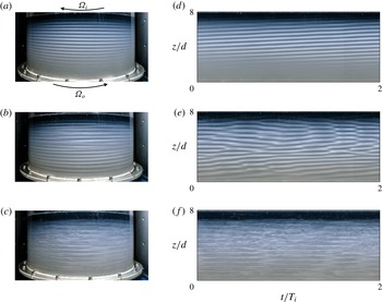
(a–c) Flow visualizations and (d–f) spatio-temporal diagrams for fixed outer Reynolds and Froude numbers
 $Re_{o}=-415$
,
 $F_{o}=-0.033$
and for (a,d)
 $Re_{i}=1056$
, (b,e)
 $Re_{i}=1219$
and (c,f)
 $Re_{i}=2203$
. The arrows in (a) indicate the direction of rotation of the outer and inner cylinders.

3 Experimental observations
We first describe the different flow regimes observed for counter-rotating cylinders. Figure 1(a–c) shows examples of flow visualizations for the outer Reynolds number
 $Re_{o}=-415$
(corresponding to
 $F_{o}=-0.033$
) and for three different inner Reynolds numbers
 $Re_{i}=1056$
, 1219 and 2203. As mentioned previously, the associated inner Froude number can be computed from the relation
 $F_{i}=F_{o}Re_{i}/(\unicode[STIX]{x1D702}Re_{o})$
. Corresponding
 $z$
–
 $t$
spatio-temporal diagrams are also displayed in figure 1(d–f) over two periods of rotation of the inner cylinder
 $2T_{i}$
, where
 $T_{i}=2\unicode[STIX]{x03C0}/\unicode[STIX]{x1D6FA}_{i}$
. They have been extracted from a vertical line in the middle of the flow visualizations. In all the flow visualizations displayed in the following, the outer cylinder rotates from left to right in the anti-clockwise direction as indicated by the arrow in figure 1(a). For
 $Re_{i}=1056$
(figure 1
a), we can see regular bands as observed for the Taylor vortices of the centrifugal instability (Taylor Reference Taylor1923; Boubnov et al.
Reference Boubnov, Gledzer and Hopfinger1995). Although the bands seem horizontal, they are slightly inclined downward from left to right, meaning that the pattern is actually a left-handed helical mode but with a low azimuthal wavenumber. A slight upward inclination of the bands can be seen also in the spatio-temporal diagram (figure 1
 $d$
). Such instability occurs when
 $Re_{i}>Re_{c}=915$
for
 $Re_{o}=-415$
. At the critical inner Reynolds number, the pattern appears first in the top part as also observed by Withjack & Chen (Reference Withjack and Chen1974). This is because the viscosity increases as the salt concentration increases implying that the local Reynolds numbers are slightly higher in the upper part of the flow than in the lower part. The pattern then invades the whole fluid as the inner Reynolds number is further increased. For
 $Re_{i}=1219$
(figure 1
b), the bands are no longer regular but move up and down and sometimes merge as clearly seen in the space–time diagram (figure 1
e). When
 $Re_{i}>1508$
, the flow becomes chaotic and small-scale turbulent structures are superimposed on the bands, first in the upper part of the flow as shown in figure 1(c,f). These small-scale turbulent structures spread over the entire domain as
 $Re_{i}$
is increased further.
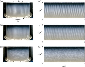
(a–c) Flow visualizations and (d–f) spatio-temporal diagrams for fixed outer Reynolds and Froude numbers
 $Re_{o}=1885$
,
 $F_{o}=0.148$
and for (a,d)
 $Re_{i}=2308$
, (b,e)
 $Re_{i}=2595$
and (c,f)
 $Re_{i}=2924$
. The arrows in (a) indicate the direction of rotation of the outer and inner cylinders.

A second series of flow visualizations and spatio-temporal diagrams are displayed in figure 2 for the regime of co-rotation for the outer Reynolds number
 $Re_{o}=1885$
(corresponding to
 $F_{o}=0.148$
) and for three different inner Reynolds numbers
 $Re_{i}=2308$
, 2595 and 2924. As seen in figure 2
 $(a)$
, the primary instability is now highly non-axisymmetric. Such a mode is similar to the one observed by Le Bars & Le Gal (Reference Le Bars and Le Gal2007) for the strato-rotational instability except that the azimuthal wavenumber in their experiments was lower
 $m=1{-}4$
. However, the gap ratio of their set-up is smaller
 $\unicode[STIX]{x1D702}=0.8$
and the Froude number is also higher
 $F_{i}=0.5$
than in the present experiment where
 $F_{i}=0.2$
. Interestingly, Leclercq et al. (Reference Leclercq, Nguyen and Kerswell2016a
) also report a high dominant azimuthal wavenumber
 $m=11$
at instability onset when
 $\unicode[STIX]{x1D707}\gtrsim 0.5$
for
 $\unicode[STIX]{x1D702}=0.9$
and
 $F_{i}=0.2$
.
When the inner Reynolds number is increased further above
 $Re_{i}=2420$
, the mode shape is still regular in space and time but becomes slightly more complex (figure 2
b,e). In particular, the spatio-temporal diagram exhibits coil-like structures as observed by Ibanez et al. (Reference Ibanez, Swinney and Rodenborn2016) for a fixed outer cylinder, i.e.
 $Re_{o}=0$
. The flow becomes disordered when the inner Reynolds number is increased further above
 $Re_{i}=2755$
. As shown in figure 2(c,f) for
 $Re_{i}=2924$
, small-scale turbulent structures are superimposed on the instability pattern.
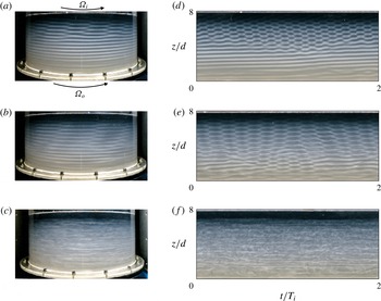
(a–c) Flow visualizations and (d–f) spatio-temporal diagrams for fixed outer Reynolds and Froude numbers
 $Re_{o}=209$
,
 $F_{o}=0.016$
and for (a,d)
 $Re_{i}=1175$
, (b,e)
 $Re_{i}=1466$
and (c,f)
 $Re_{i}=2719$
. The arrows in
 $(a)$
indicate the direction of rotation of the outer and inner cylinders.

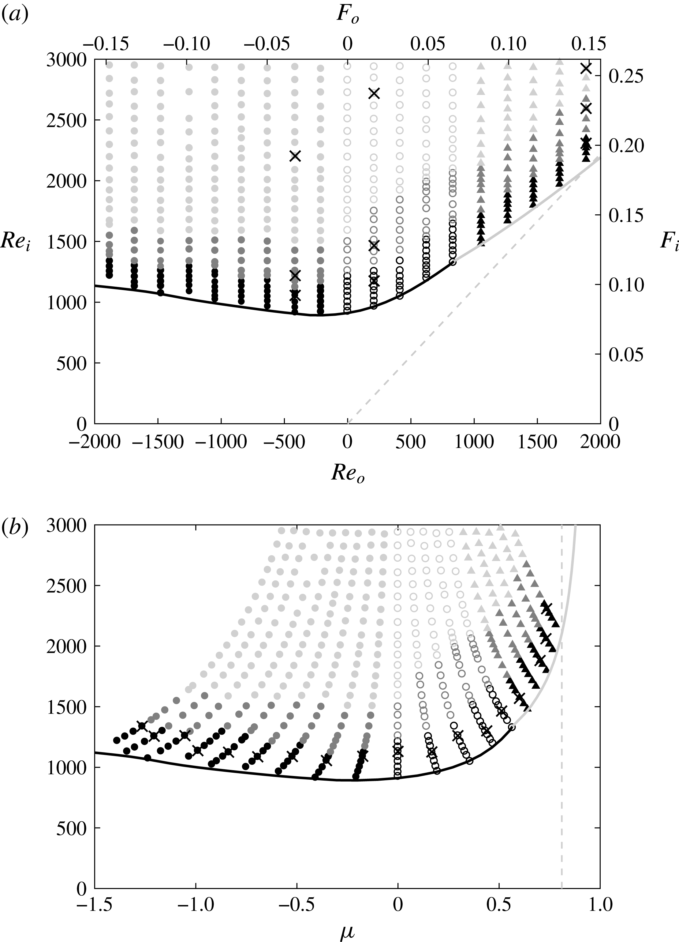
Map of the flow regimes in the parameter spaces (a)
 $(Re_{o},Re_{i})$
and (b)
 $(\unicode[STIX]{x1D707},Re_{i})$
. The labels on the upper and right axes in (a) indicate the corresponding Froude numbers
 $F_{o}$
and
 $F_{i}$
. The different grey scales indicate the flow regimes observed in the experiments: primary instability (black), secondary modes (dark grey) and turbulence (grey), whereas the different symbols indicate the nature of the primary mode: weakly non-axisymmetric mode (filled circles), highly non-axisymmetric mode (triangles) and mixed modes (empty circles). The grey dashed lines represent the Rayleigh line
 $\unicode[STIX]{x1D707}=\unicode[STIX]{x1D702}^{2}$
. The thick solid line represents the neutral stability curve determined numerically over all axial and azimuthal wavenumbers for
 $N=3.18~\text{rad}~\text{s}^{-1}$
. The line is black when the primary instability occurs at low azimuthal wavenumbers (
 $m\leqslant 4$
) and grey otherwise (
 $m>4$
). The black crosses in (a) indicate the parameters of the flow visualizations displayed in figures 1, 2 and 3, while the crosses in (b) indicate the values of
 $Re_{i}$
for which we have performed the comparison between experimental and numerical results displayed in figures 14 and 15(b).

We now turn our attention to the flows observed for an intermediate value of the outer Reynolds number
 $Re_{o}=209$
(
 $F_{o}=0.016$
). As seen in figure 3(a,d), a highly non-axisymmetric mode and a weakly non-axisymmetric mode similar to those in figures 2(a) and 1(a) are observed simultaneously in the upper and lower parts of the flow, respectively. However, the weakly non-axisymmetric mode is now a right-handed helix instead of a left-handed helix as in figure 1(a). In addition, we observe in the spatio-temporal diagram (figure 3
d) that the vertical extent of the region where the highly non-axisymmetric mode is present, widens near
 $t=T_{i}$
and then shrinks at
 $t=2T_{i}$
. This oscillation has been observed to occur regularly (not shown) over a long time with an approximate time period of
 $2T_{i}$
. Such a mixed mode appears in two steps. When
 $Re_{i}$
is just above the critical inner Reynolds number, the weakly non-axisymmetric mode first develops at the top. When
 $Re_{i}$
is further increased, it progressively invades the flow downwards while, concomitantly, the highly non-axisymmetric mode appears at the top as observed in figure 3(a,d). For
 $Re_{i}=1466$
(figure 3
b,e), the region of the highly non-axisymmetric mode widens in the axial direction but weakly non-axisymmetric bands are still observed near the bottom. An oscillation with a period around
 $2T_{i}$
of the vertical extent of each region continues to be observed as in figure 3(d). When the inner Reynolds number is increased further as
 $Re_{i}>1843$
, transition to small-scale turbulence occurs and two different modes are no longer distinguishable (figure 3
c,f).
Figure 4(a) summarizes all the experimental observations (symbols) in the parameter space
 $(Re_{o},Re_{i})$
and shows the neutral stability curve computed numerically for
 $N=3.18~\text{rad}~\text{s}^{-1}$
and
 $\unicode[STIX]{x1D708}=\unicode[STIX]{x1D708}_{0}$
(thick line). The corresponding Froude numbers
 $(F_{o},F_{i})$
are indicated on the top and right axes. This instability map is also represented as a function of
 $(\unicode[STIX]{x1D707},Re_{i})$
in figure 4(b) to ease the comparison with previous studies where such representation is used (Shalybkov & Rüdiger Reference Shalybkov and Rüdiger2005; Le Bars & Le Gal Reference Le Bars and Le Gal2007; Ibanez et al.
Reference Ibanez, Swinney and Rodenborn2016; Leclercq et al.
Reference Leclercq, Nguyen and Kerswell2016a
). The weakly non-axisymmetric mode (filled circles) has been observed in all the counter-rotating cases
 $Re_{o}<0$
(equivalently
 $\unicode[STIX]{x1D707}<0$
) whereas the highly non-axisymmetric mode (triangles) has been observed for co-rotation for sufficiently large outer Reynolds number
 $Re_{o}>840$
(
 $\unicode[STIX]{x1D707}>0.57$
). In between:
 $0\leqslant Re_{0}\leqslant 840$
(
 $0\leqslant \unicode[STIX]{x1D707}\leqslant 0.57$
), the two modes are simultaneously observed (empty circles). No symbol has been plotted when the flow is stable so that the lowest dots delineate the experimental neutral stability curve above which an instability first appears in the top part of the flow. These points are close to the overall neutral stability curve determined numerically over all axial and azimuthal wavenumbers (thick line). This neutral curve is black when the dominant mode at onset has a low azimuthal wavenumber (
 $m\leqslant 4$
) and grey otherwise (
 $m>4$
). The grey portion of the neutral curve agrees well with the regime where the highly non-axisymmetric mode is observed in the experiments. For negative
 $Re_{o}$
, the black colour of the curve is also consistent with the experimental observations of weakly non-axisymmetric modes. In contrast, in the intermediate range
 $0\leqslant Re_{o}\leqslant 840$
, the curve is black while both highly non-axisymmetric modes and weakly non-axisymmetric modes have been observed simultaneously in the experiments. In the next section, we will see that this apparent discrepancy comes from the fact that the dominant mode is weakly non-axisymmetric on the marginal stability curve whereas, just above it, a second mode, which is highly non-axisymmetric, becomes also unstable. We can further remark that the critical inner Reynolds number is at least
 $Re_{i}\gtrsim 900$
and thus significantly larger than in previous experimental studies. For example, Shalybkov & Rüdiger (Reference Shalybkov and Rüdiger2005) and Le Bars & Le Gal (Reference Le Bars and Le Gal2007) report
 $Re_{i}\gtrsim 200$
for
 $\unicode[STIX]{x1D702}\sim 0.8$
and
 $F_{i}=0.5$
while Leclercq et al. (Reference Leclercq, Nguyen and Kerswell2016a
) found
 $Re_{i}\gtrsim 300$
for
 $\unicode[STIX]{x1D702}=0.9$
and
 $F_{i}=0.2$
. However, the stratification is stronger in the present experiments since the inner Froude number is below
 $F_{i}=0.1$
for
 $Re_{i}=900$
.
Away from the marginal stability curve (figure 4), the dark grey and grey symbols indicate the parameters for which secondary modes and turbulence have been observed. While there is a large variety of distinct flow states when the fluid is not stratified (Andereck et al.
Reference Andereck, Liu and Swinney1986), only the main flow regimes illustrated in figures 1–3 have been distinguished here for a strong stratification. Some series of experiments have been repeated several times and the observations have been found to be reproducible from one experiment to the other. However, experiments performed with a different protocol, such as for decreasing
 $\unicode[STIX]{x1D6FA}_{i}$
, could lead to different observations because of subcritical transitions and hysteresis. Although further studies of the nonlinear dynamics of the primary and secondary modes and the transition to turbulence would be of interest, this is left for future work and we shall concentrate in the next section on a quantitative comparison between the characteristics (temporal frequency, axial and azimuthal wavenumbers) of the primary modes observed experimentally and predicted by the linear stability analysis. This will allow us to prove that the weakly and highly non-axisymmetric modes originate from the centrifugal and strato-rotational instabilities, respectively.
4 Comparison between linear stability results and experimental observations of the primary instability
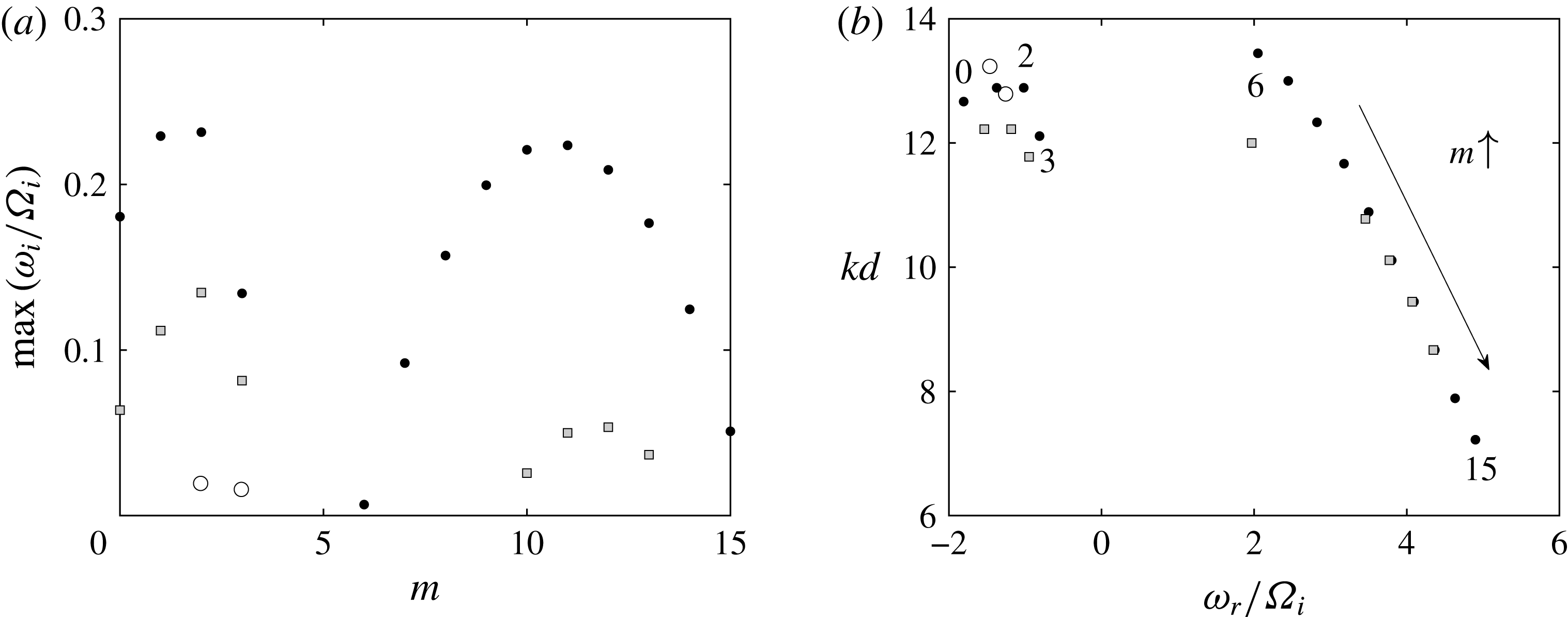
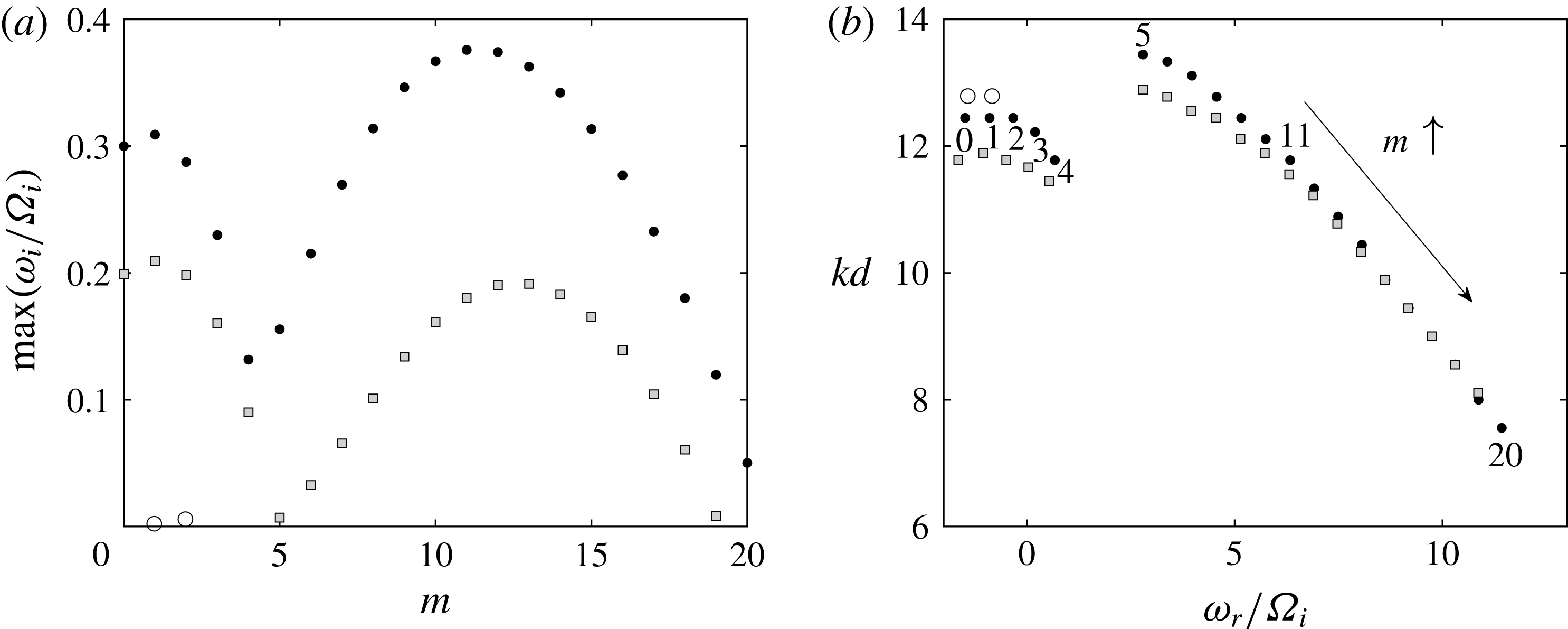
Figure 5(a) shows the maximum growth rate as a function of the azimuthal wavenumber determined numerically over all axial wavenumbers
 $k$
for the fixed outer Froude number
 $F_{o}=-0.033$
pertaining to figure 1 and for three sets of Reynolds numbers
 $(Re_{o},Re_{i})$
. The values (
 $Re_{o}=-415$
,
 $Re_{i}=915$
) (empty circles) correspond to the critical parameters found in the experiments for
 $F_{o}=-0.033$
while the values (
 $Re_{o}=-415$
,
 $Re_{i}=1056$
) (black dots) correspond to the reference Reynolds numbers of the primary instability shown in figure 1(a). In addition, we display the growth rate for the same Froude number but for the lower Reynolds numbers (
 $Re_{o}=-346$
,
 $Re_{i}=880$
) (grey squares) computed with the viscosity
 $\unicode[STIX]{x1D708}=1.2\unicode[STIX]{x1D708}_{0}$
. These values are the local Reynolds numbers at mid-depth in the experiment of figure 1(a) while the reference Reynolds numbers (
 $Re_{o}=-415$
,
 $Re_{i}=1056$
) correspond to the local Reynolds numbers at the top since they are based on the viscosity of pure water.
(a) Maximum growth rate as a function of the azimuthal wavenumber and (b) corresponding axial wavenumber as a function of the frequency for a fixed outer Froude number
 $F_{o}=-0.033$
and for
 $(Re_{o},Re_{i})=(-415,915)$
(empty circles), (
 $-$
415, 1056) (black dots) and (
 $-$
346, 880) (grey squares). The numbers near the dots in (b) indicate the corresponding azimuthal wavenumber for
 $(Re_{o},Re_{i})=(-415,1056)$
.

The maximum growth rate is only slightly positive for
 $m=2$
and
 $m=3$
for (
 $Re_{o}=-415$
,
 $Re_{i}=915$
) confirming that we are very close to the neutral stability curve. When
 $Re_{i}$
is increased to
 $1056$
for
 $Re_{o}=-415$
, the growth rate becomes much larger and a second growth rate peak arises at large azimuthal wavenumber
 $m=11$
. However, the overall maximum growth rate is still reached by the first peak at
 $m=2$
. For (
 $Re_{o}=-346$
,
 $Re_{i}=880$
), the growth rate curve is lower but similar. The corresponding frequency and axial wavenumber of the unstable modes for these three sets of Reynolds numbers are displayed in figure 5(b) for each azimuthal wavenumber. Two distinct branches can be seen: one for
 $m\leqslant 3$
with negative frequency and the other for
 $m\geqslant 6$
with positive frequency
 $\unicode[STIX]{x1D714}_{r}/\unicode[STIX]{x1D6FA}_{i}>2$
.
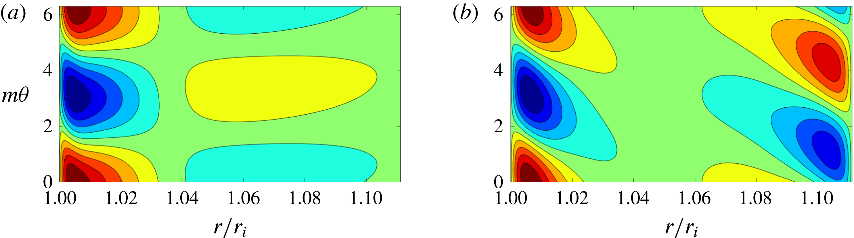
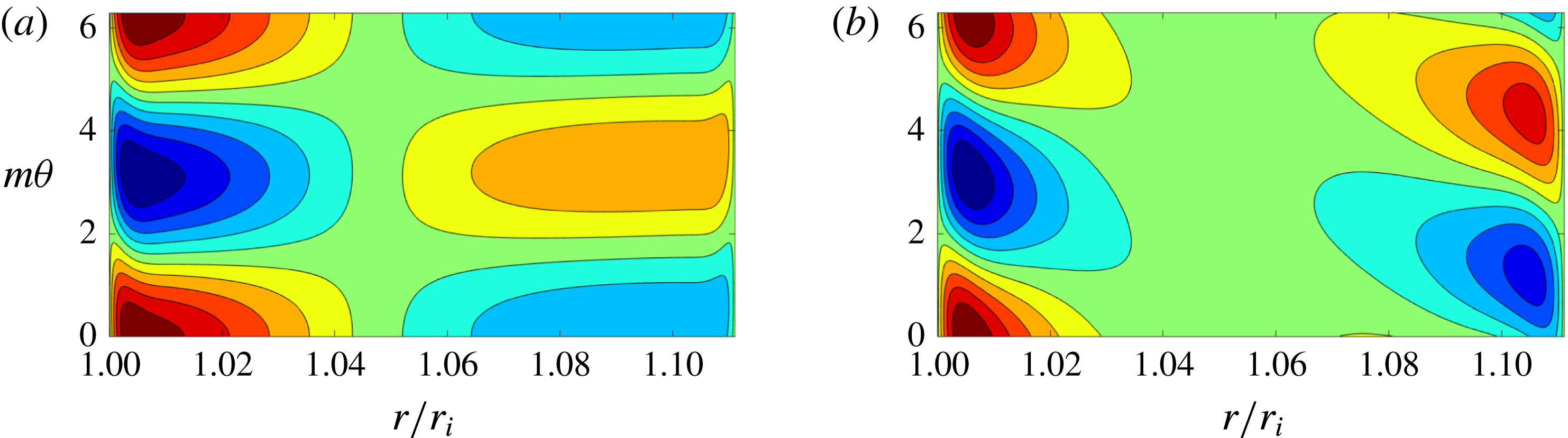
Contours of the vertical velocity
 $\text{Re}[u_{z}(r)\exp (\text{i}m\unicode[STIX]{x1D703})]$
of the dominant eigenmode for
 $Re_{o}=-415$
,
 $Re_{i}=1056$
,
 $F_{o}=-0.033$
and for (a)
 $m=2$
and
 $(b)$
 $m=11$
. Only one wavelength is represented along the azimuthal direction. The contours are normalized by the maximum value of
 $u_{z}$
and the contour interval is 0.2.

The dominant eigenmodes for
 $m=2$
and
 $m=11$
are also different as illustrated by their axial velocity perturbation
 $u_{z}$
in figure 6. For
 $m=2$
, there are weak sheared waves localized near the inner cylinder while, for
 $m=11$
, two out-of-phase waves are trapped near each cylinder. These shapes are very similar to those found by Park et al. (Reference Park, Billant and Baik2017) for the centrifugal and strato-rotational instabilities, respectively, demonstrating the different origin of the two growth rate peaks. These results contradict Leclercq et al. (Reference Leclercq, Nguyen and Kerswell2016a
) who argued that the centrifugal and strato-rotational instabilities are indistinguishable at onset. This point will be discussed in § 5.
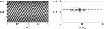
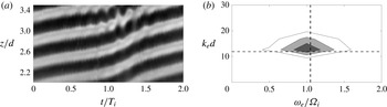
In order to compare these results to the characteristics of the experimentally observed mode in figure 1(a,d), a two-dimensional Fourier transform has been applied to the grey-scale spatio-temporal diagram
 $g(t,z)$
(Le Bars & Le Gal Reference Le Bars and Le Gal2007)
 $$\begin{eqnarray}g(t,z)=\mathop{\sum }_{k_{e}}\mathop{\sum }_{\unicode[STIX]{x1D714}_{e}}{\hat{g}}(\unicode[STIX]{x1D714}_{e},k_{e})\exp \left[\text{i}(k_{e}z-\unicode[STIX]{x1D714}_{e}t)\right],\end{eqnarray}$$
where
 ${\hat{g}}$
is the Fourier coefficient,
 $k_{e}$
the axial wavenumber and
 $\unicode[STIX]{x1D714}_{e}$
the temporal frequency. The spatio-temporal diagram
 $g(t,z)$
(figure 1
d) has been first cropped to keep only the portion where the pattern is the clearest as illustrated in 7(a). Linear trends of the grey-scale level, that are mostly due to non-uniform concentration of mica powder and lighting, have been also removed.
(a) Grey-scale spatio-temporal diagram
 $g(t,z)$
extracted from figure 1
 $(d)$
(
 $Re_{o}=-415$
,
 $Re_{i}=1056$
,
 $F_{o}=-0.033$
). (b) Contours of the corresponding Fourier coefficient
 $|{\hat{g}}(\unicode[STIX]{x1D714}_{e},k_{e})|$
. The horizontal and vertical dashed lines represent the axial wavenumber
 $kd$
and the frequency
 $|\unicode[STIX]{x1D714}_{r}/\unicode[STIX]{x1D6FA}_{i}|$
of the most unstable mode
 $m=2$
obtained from the linear stability analysis for
 $Re_{o}=-415$
,
 $Re_{i}=1056$
,
 $F_{o}=-0.033$
(figure 5).

The resulting Fourier coefficient
 $|{\hat{g}}|$
is plotted as a function of
 $(\unicode[STIX]{x1D714}_{e}/\unicode[STIX]{x1D6FA}_{i},k_{e}d)$
in figure 7(b). The maximum of
 $|{\hat{g}}|$
is reached at
 $(\unicode[STIX]{x1D714}_{e}/\unicode[STIX]{x1D6FA}_{i},k_{e}d)=(1.0,14.6)$
which is close to the axial wavenumber and frequency
 $(|\unicode[STIX]{x1D714}_{r}/\unicode[STIX]{x1D6FA}_{i}|,kd)=(1.02,13.22)$
(dashed lines) of the most amplified azimuthal wavenumber
 $m=2$
found in the linear stability analysis for
 $Re_{o}=-415$
,
 $Re_{i}=1056$
,
 $F_{o}=-0.033$
. This proves that the weakly non-axisymmetric mode observed in figure 1(a) is due to the centrifugal instability. Alternatively, we have also directly measured the axial wavelength and the period of the mode by simply measuring the length in axial direction
 $z$
and in time
 $t$
of a given number of repeated patterns in figure 7. This method yields
 $(\unicode[STIX]{x1D714}_{e}/\unicode[STIX]{x1D6FA}_{i},k_{e}d)=(0.89,14.4)$
which are close to the values obtained from the Fourier transform. In appendix A, we show that there is always a good agreement between such direct measurements and the results of the Fourier transform. Hence, only the results of the Fourier transform will be presented in the following.
We can further remark that the linear stability analysis predicts that, if a perturbation with positive wavenumbers
 $(m,k)$
is unstable, then the perturbations with wavenumbers
 $(m,-k)$
,
 $(-m,k)$
and
 $(-m,-k)$
are also unstable with the same growth rate due to the symmetry of the linear equations. This indicates that there should be two types of unstable modes: right-handed and left-handed helical modes corresponding to
 $mk<0$
and
 $mk>0$
, respectively. However, figure 1(a) shows that only a left-handed helical mode is observed since the lines of constant phase
 $\unicode[STIX]{x1D719}=m\unicode[STIX]{x1D703}+kz-\unicode[STIX]{x1D714}_{r}t$
are inclined downward in the positive
 $\unicode[STIX]{x1D703}$
direction. This selection is most probably due to nonlinear effects as observed in homogeneous fluids (Tagg et al.
Reference Tagg, Edwards, Swinney and Marcus1989). It can be also checked that the sign of the rescaled frequency
 $\unicode[STIX]{x1D714}_{r}/\unicode[STIX]{x1D6FA}_{i}$
is negative in the experiments in agreement with the results of the stability analysis for the centrifugal modes (figure 5
b). Indeed, the upward inclination of the lines of constant phase
 $\unicode[STIX]{x1D719}$
in the
 $(t,z)$
spatio-temporal diagram (figure 1
d) implies that
 $\unicode[STIX]{x1D714}_{r}$
is positive. The rescaled frequency
 $\unicode[STIX]{x1D714}_{r}/\unicode[STIX]{x1D6FA}_{i}$
is therefore negative since
 $\unicode[STIX]{x1D6FA}_{i}$
is directed in the negative direction in figure 1(a).
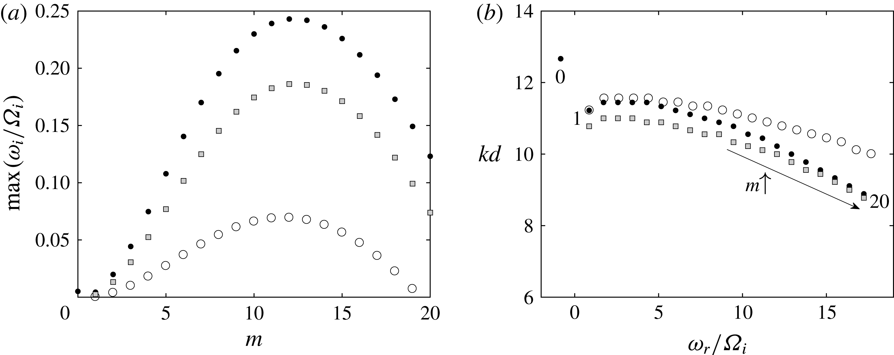
Same as figure 5 except for the fixed outer Froude number
 $F_{o}=0.148$
and for
 $(Re_{o},Re_{i})=(1885,1958)$
(empty circles), (1885, 2308) (black dots) and (1571, 1923) (grey squares). The numbers near the dots in (b) indicate the corresponding azimuthal wavenumber for
 $(Re_{o},Re_{i})=(1885,2308)$
.

Similarly, figure 8(a) shows the maximum growth rate as a function of the azimuthal wavenumber computed for the outer Froude number
 $F_{o}=0.148$
corresponding to figure 2. The inner Reynolds numbers
 $Re_{i}=1958$
(empty circles) is the experimental critical Reynolds number for
 $Re_{o}=1885$
while (
 $Re_{o}=1885,Re_{i}=2308$
) (black dots) are the reference Reynolds numbers of the highly non-axisymmetric mode displayed in figure 2(a). As before, we also show the growth rate for (
 $Re_{o}=1571,Re_{i}=1923$
) (grey squares) which pertain to the flow at mid-depth in figure 2(a). For the three sets of Reynolds numbers, there is now a single growth rate peak at
 $m=12$
. The dominant eigenmode for
 $m=12$
(not shown) is similar to the one displayed in figure 6(b) meaning that the instability is strato-rotational. The corresponding axial wavenumber and frequency of the dominant mode for each azimuthal wavenumber are shown in figure 8(b). There is a single branch except for (
 $Re_{o}=1885,Re_{i}=2308$
) where the axisymmetric mode
 $m=0$
is also slightly unstable. This is the only azimuthal wavenumber for which the centrifugal instability is dominant because the angular velocity ratio
 $\unicode[STIX]{x1D707}=0.735$
is just below the Rayleigh line
 $\unicode[STIX]{x1D707}=\unicode[STIX]{x1D702}^{2}$
as seen in figure 4(a).
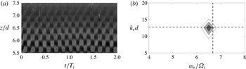
Figure 9(a) shows a grey-scale spatio-temporal diagram extracted from figure 2(d). The resulting Fourier transform (figure 9
 $b$
) exhibits a peak at
 $(\unicode[STIX]{x1D714}_{e}/\unicode[STIX]{x1D6FA}_{i},k_{e}d)=(9.5,12.6)$
. The peak is less compact and more distorted than in figure 7(b), probably because of the defects seen around
 $t/T_{i}=0.6$
and
 $t/T_{i}=1.8$
in figure 9(a). Nevertheless, this peak is close to the frequency and wavenumber
 $(\unicode[STIX]{x1D714}_{r}/\unicode[STIX]{x1D6FA}_{i},kd)=(10.33,10.56)$
(dashed lines) of the azimuthal wavenumber
 $m=12$
predicted numerically for
 $Re_{o}=1885$
,
 $Re_{i}=2308$
,
 $F_{o}=0.148$
.
(a) Grey-scale spatio-temporal diagram
 $g(t,z)$
extracted from figure 2(d) (
 $Re_{o}=1885$
,
 $Re_{i}=2308$
,
 $F_{o}=0.148$
). (b) Contours of the corresponding Fourier coefficient
 $|{\hat{g}}(\unicode[STIX]{x1D714}_{e},k_{e})|$
. The horizontal and vertical dashed lines represent the axial wavenumber
 $kd$
and the frequency
 $\unicode[STIX]{x1D714}_{r}/\unicode[STIX]{x1D6FA}_{i}$
of the most unstable mode
 $m=12$
obtained from the linear stability analysis for
 $Re_{o}=1885$
,
 $Re_{i}=2308$
,
 $F_{o}=0.148$
(figure 8).

Same as figure 5 except for the fixed outer Froude number
 $F_{o}=0.016$
and for (
 $Re_{o}=209$
,
 $Re_{i}=968$
) (empty circles), (
 $Re_{o}=209$
,
 $Re_{i}=1175$
) (black dots) and (
 $Re_{o}=174$
,
 $Re_{i}=979$
) (grey squares). The numbers near the dots in (b) indicate the corresponding azimuthal wavenumber for
 $(Re_{o},Re_{i})=(209,1175)$
.

Finally, figure 10(a) shows the maximum growth rate as a function of the azimuthal wavenumber for the intermediate outer Froude number
 $F_{o}=0.016$
corresponding to figure 3. At the critical inner Reynolds number
 $Re_{i}=968$
found experimentally for
 $Re_{o}=209$
, the maximum growth rate (empty circles) is reached at
 $m=2$
but is very low. For the Reynolds numbers (
 $Re_{o}=209$
,
 $Re_{i}=1175$
) (black dots) and (
 $Re_{o}=174$
,
 $Re_{i}=979$
) (grey squares) characterizing the flow of figure 3(a) at the top and at mid-depth, respectively, the growth rate becomes large and exhibits two comparable maxima as in figure 5(a). Interestingly, the peak at
 $m=11$
is slightly higher than the one at
 $m=1$
for (
 $Re_{o}=209$
,
 $Re_{i}=1175$
) while it is the opposite for (
 $Re_{o}=174$
,
 $Re_{i}=979$
). Two separate frequency branches can be also seen in figure 10(b): one with frequency
 $\unicode[STIX]{x1D714}_{r}/\unicode[STIX]{x1D6FA}_{i}<0.7$
for
 $m\leqslant 4$
and the other with frequency
 $\unicode[STIX]{x1D714}_{r}/\unicode[STIX]{x1D6FA}_{i}>2.7$
for
 $m\geqslant 5$
.
Contours of the vertical velocity
 $Re[u_{z}(r)\exp (\text{i}m\unicode[STIX]{x1D703})]$
of the dominant eigenmode for
 $Re_{o}=209$
,
 $Re_{i}=1175$
,
 $F_{o}=0.016$
and for (a)
 $m=1$
and (b)
 $m=11$
. Only one wavelength is represented along the azimuthal direction. The contours are normalized by the maximum value of
 $u_{z}$
and the contour interval is 0.2.

The most unstable eigenmodes (figure 11) corresponding to each of these two branches are similar to those displayed in figure 6. This demonstrates that the low
 $m$
branch corresponds to the centrifugal instability while the high
 $m$
branch is due to the strato-rotational instability as in figure 5.
(a) Grey-scale spatio-temporal diagram
 $g(t,z)$
extracted from the upper part of figure 3(d). (b) Contours of the corresponding Fourier coefficient
 $|{\hat{g}}(\unicode[STIX]{x1D714}_{e},k_{e})|$
. The horizontal and vertical dashed lines represent the axial wavenumber
 $kd$
and the frequency
 $\unicode[STIX]{x1D714}_{r}/\unicode[STIX]{x1D6FA}_{i}$
of the most unstable mode
 $m=11$
obtained from the linear stability analysis for
 $Re_{o}=209$
,
 $Re_{i}=1175$
,
 $F_{o}=0.016$
(figure 10).

(a) Grey-scale spatio-temporal diagram
 $g(t,z)$
extracted from the lower part of figure 3(d). (b) Contours of the corresponding Fourier coefficient
 $|{\hat{g}}(\unicode[STIX]{x1D714}_{e},k_{e})|$
. The horizontal and vertical dashed lines represent the axial wavenumber
 $kd$
and the frequency
 $|\unicode[STIX]{x1D714}_{r}/\unicode[STIX]{x1D6FA}_{i}|$
of the mode
 $m=1$
obtained from the linear stability analysis for
 $Re_{o}=174$
,
 $Re_{i}=979$
,
 $F_{o}=0.016$
(figure 10).

To obtain the characteristics of the two different modes observed in the experiments, the Fourier transform has been applied separately to the upper and lower parts of the spatio-temporal diagram in figure 3(d). The dominant frequency and axial wavenumber of the upper part (figure 12) and lower part (figure 13) are
 $(\unicode[STIX]{x1D714}_{e}/\unicode[STIX]{x1D6FA}_{i},k_{e}d)=(6.5,12.5)$
and
 $(\unicode[STIX]{x1D714}_{e}/\unicode[STIX]{x1D6FA}_{i},k_{e}d)=(1.0,12.7)$
, respectively. We can see that they are very close to the computed frequency and axial wavenumber
 $(|\unicode[STIX]{x1D714}_{r}/\unicode[STIX]{x1D6FA}_{i}|,kd)=(6.3,11.8)$
(dashed lines) of the
 $m=11$
mode for
 $Re_{o}=209$
,
 $Re_{i}=1175$
,
 $F_{o}=0.016$
(figure 12
b) and
 $(|\unicode[STIX]{x1D714}_{r}/\unicode[STIX]{x1D6FA}_{i}|,kd)=(1.1,11.9)$
(dashed lines) of the
 $m=1$
mode for
 $Re_{o}=174$
,
 $Re_{i}=979$
,
 $F_{o}=0.016$
(figure 13
b). This confirms that the weakly and highly non-axisymmetric modes come from the centrifugal and strato-rotational instabilities, respectively. The selection of these two different instabilities in the lower and upper parts of the fluid can be understood by considering the effect of the Reynolds numbers. Indeed, figure 10 shows that the strato-rotational instability is slightly more unstable than the centrifugal instability for the Reynolds numbers (
 $Re_{o}=209$
,
 $Re_{i}=1175$
) characterizing the top flow while the centrifugal instability is slightly more dominant for the local Reynolds numbers at mid-depth (
 $Re_{o}=174$
,
 $Re_{i}=979$
). This exchange is due to the fact that the growth rate of the strato-rotational instability decreases faster than the one of the centrifugal instability when the Reynolds number decreases. The higher dominant azimuthal wavenumber of the strato-rotational instability is probably responsible for this stronger viscous damping. Hence, because the local Reynolds number decreases downward due to the salinity gradient, there is a vertical level where a switchover between the two instabilities occurs. When these two instabilities are simultaneously observed in experiments, strictly speaking, the strato-rotational instability develops over the centrifugal instability as pointed out by one referee. Therefore, the strato-rotational instability should be considered as a secondary instability in this case.
In contrast, only the centrifugal instability is observed in figure 1(a,d) although the strato-rotational instability has a comparable maximum growth rate (figure 5). The difference from the previous case is that the centrifugal instability is already slightly more unstable than the strato-rotational instability for the reference Reynolds numbers (
 $Re_{o}=-415$
,
 $Re_{i}=1056$
) which pertain to the top fluid. Thus, the centrifugal instability remains dominant further downward as the local Reynolds number decreases.
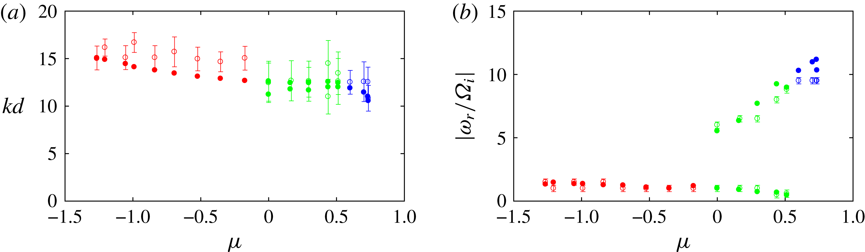
Comparison between the linear stability results (dots) and the experimental observations (empty circles with error bars) for (a) the axial wavenumber
 $kd$
and (b) the frequency
 $|\unicode[STIX]{x1D714}_{r}/\unicode[STIX]{x1D6FA}_{i}|$
. The symbols are coloured in red, green and blue when the dominant instability is centrifugal, mixed and strato-rotational, respectively. The error bars correspond to
 $\unicode[STIX]{x0394}(k_{e}d)$
in (a) and
 $\unicode[STIX]{x0394}(\unicode[STIX]{x1D714}_{e}/\unicode[STIX]{x1D6FA}_{i})$
in (b), where
 $\unicode[STIX]{x0394}k_{e}$
and
 $\unicode[STIX]{x0394}\unicode[STIX]{x1D714}_{e}$
are the wavenumber and frequency resolutions of the Fourier transform (4.1).

The comparison between the axial wavenumber and frequency of the computed and observed modes has been performed for the values of the outer Reynolds number
 $Re_{o}$
investigated in the experiments. For each case, the inner Reynolds number
 $Re_{i}$
of the analysed mode has been chosen to lie around the middle of the primary instability region (indicated by black
 $+$
symbols in figure 4
b) so that the pattern is clearly defined. The results are summarized in figures 14(a) and 14(b) as a function of the angular velocity ratio
 $\unicode[STIX]{x1D707}$
. We can see that there is always a good agreement between the experimental (empty circles) and numerical (dots) results. The symbols are coloured in red, green and blue when the dominant instability is centrifugal, mixed and strato-rotational, respectively. The axial wavenumber (figure 14
a) varies smoothly and only weakly between these three regimes whereas there is a large frequency jump (figure 14
b) between the centrifugal and strato-rotational instability modes.
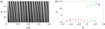
(a) Spatio-temporal diagram in the directions
 $\unicode[STIX]{x1D703}$
–
 $t$
extracted from a horizontal line at
 $z/d=6$
in figure 2(a) over the angle
 $\unicode[STIX]{x0394}\unicode[STIX]{x1D703}=\unicode[STIX]{x03C0}/16$
. (b) Comparison between the linear stability results (dots) and the experimental observations (empty circles with error bars) for the azimuthal wavenumber
 $m$
. The error bars correspond to
 $\unicode[STIX]{x0394}(\unicode[STIX]{x1D714}_{e}\unicode[STIX]{x0394}t/\unicode[STIX]{x0394}\unicode[STIX]{x1D703})$
where
 $\unicode[STIX]{x0394}\unicode[STIX]{x1D714}_{e}$
is the frequency resolution of the Fourier transform (4.1).

In order to make a more comprehensive comparison, the azimuthal wavenumber of the observed modes has been further estimated from spatio-temporal diagrams in the
 $\unicode[STIX]{x1D703}$
and
 $t$
directions (see the example in figure 15
 $a$
). The diagrams have been taken over the angle
 $\unicode[STIX]{x0394}\unicode[STIX]{x1D703}=\unicode[STIX]{x03C0}/16$
, i.e. the angle between two bolts seen in the flow visualizations (figures 1–3
a–c). A small angle has been chosen in order to minimize curvature effects but this precludes the use of a Fourier transform as before since the azimuthal variations over
 $\unicode[STIX]{x0394}\unicode[STIX]{x1D703}$
are weak. Instead, the azimuthal wavenumber has been retrieved from the slope of the pattern
 $\unicode[STIX]{x0394}t/\unicode[STIX]{x0394}\unicode[STIX]{x1D703}$
by using the formula
 $m=\unicode[STIX]{x1D714}_{e}\unicode[STIX]{x0394}t/\unicode[STIX]{x0394}\unicode[STIX]{x1D703}$
, where
 $\unicode[STIX]{x1D714}_{e}$
is the frequency measured previously (figure 14
b). As shown in figure 15(b), these measurements are in good agreement with the dominant azimuthal wavenumbers predicted by the linear stability analysis. The dominant azimuthal wavenumbers are always around
 $m=1{-}2$
for the centrifugal instability and around
 $m=11{-}14$
for the strato-rotational instability. The azimuthal wavenumber together with the frequency are therefore the main distinguishing attributes of the centrifugal and strato-rotational instabilities.
5 Conclusions and discussions
In this paper, we have investigated experimentally and numerically the stability of the stably stratified Taylor–Couette flow for the Brunt–Väisälä frequency
 $N\approx 3.2~\text{rad}~\text{s}^{-1}$
and the gap ratio
 $\unicode[STIX]{x1D702}=0.9$
. The Reynolds numbers have been varied over large ranges:
 $0<Re_{i}<3000$
,
 $-2000<Re_{o}<2000$
, corresponding to angular velocity ratios in the range:
 $-1.5<\unicode[STIX]{x1D707}<0.8$
. The associated Froude numbers are small:
 $|F_{i}|<0.262$
and
 $|F_{o}|<0.157$
, meaning that the flow is always strongly stratified.
For each series of experiments, the inner angular velocity
 $\unicode[STIX]{x1D6FA}_{i}$
has been increased from zero by small steps while keeping the outer angular velocity
 $\unicode[STIX]{x1D6FA}_{o}$
constant. Above instability onset, three types of flow patterns have been observed: a weakly non-axisymmetric mode in the counter-rotating regime
 $Re_{o}<0$
(i.e.
 $\unicode[STIX]{x1D707}<0$
), a highly non-axisymmetric mode in the co-rotating regime for
 $Re_{o}>840$
(equivalent to
 $\unicode[STIX]{x1D707}>0.57$
) and both modes simultaneously in different regions of the flow in the intermediate regime
 $0\leqslant Re_{o}\leqslant 840$
(
 $0\leqslant \unicode[STIX]{x1D707}\leqslant 0.57$
). We have also described the destabilization of these patterns by the first secondary instability and the transition to small-scale turbulence as the inner Reynolds number is further increased.
These experimental observations have been compared to the results of a linear stability analysis. The experimental and numerical neutral stability curves are in good agreement. The frequency, axial wavenumber and azimuthal wavenumber of the primary modes observed slightly above the instability threshold have been also retrieved from
 $z$
–
 $t$
and
 $\unicode[STIX]{x1D703}$
–
 $t$
spatio-temporal diagrams. These measurements show that the weakly and highly non-axisymmetric modes have similar axial wavenumber but their azimuthal wavenumber and frequency are clearly different: (
 $m\sim 1{-}2$
,
 $\unicode[STIX]{x1D714}_{e}/\unicode[STIX]{x1D6FA}_{i}\sim 1{-}2$
) and (
 $m\sim 11{-}14$
,
 $\unicode[STIX]{x1D714}_{e}/\unicode[STIX]{x1D6FA}_{i}\sim 5{-}10$
), respectively. These characteristics are in good quantitative agreement with those of the dominant modes computed numerically. In addition, the linear stability analysis clearly shows that these two types of mode belong to two distinct branches with different eigenfunctions and instability mechanisms: the weakly non-axisymmetric modes correspond to the centrifugal instability while the highly non-axisymmetric modes are due to the strato-rotational instability. These two instabilities exist with a comparable growth rate over a large range of
 $Re_{o}$
and are thereby competing. The co-existence of the two instabilities in different regions of the flow for
 $0\leqslant Re_{o}\leqslant 840$
comes from the vertical variations of the local Reynolds numbers due to the salinity gradient. Indeed, the downward increase of the viscosity influences differently the growth rate of the two instabilities: the strato-rotational instability which has a higher azimuthal wavenumber is more damped than the centrifugal instability when the Reynolds numbers decrease. Thus, the strato-rotational instability, although dominant in the upper flow, is overcome by the centrifugal instability below a vertical level. For similar reasons, the centrifugal and strato-rotational instabilities are observed to first occur at instability onset in the upper region of the flow since the Reynolds number is highest there (Withjack & Chen Reference Withjack and Chen1974)
Our results contradict the conclusion of Leclercq et al. (Reference Leclercq, Nguyen and Kerswell2016a
) that the centrifugal and strato-rotational instabilities are indistinguishable at onset. However, we note that their conclusion is mostly based on the absence of discontinuity of the axial wavenumber of the dominant mode determined from a linear stability analysis for a large gap
 $\unicode[STIX]{x1D702}=0.417$
. First, it might be not sufficient to look only at discontinuities of the axial wavenumber to detect competing instabilities since they can have similar dominant axial wavenumber as found herein. Second, their results show that the dominant azimuthal wavenumber near the marginal curve is always low
 $m\sim 0{-}2$
, even above the Rayleigh line
 $\unicode[STIX]{x1D707}>\unicode[STIX]{x1D702}^{2}$
. This indicates that the centrifugal and strato-rotational instabilities are operating on similar azimuthal wavenumbers for the gap ratio
 $\unicode[STIX]{x1D702}=0.417$
. In contrast, the instability map of Leclercq et al. (Reference Leclercq, Nguyen and Kerswell2016a
) for the small gap
 $\unicode[STIX]{x1D702}=0.9$
and Froude number
 $F_{i}=0.2$
is actually consistent with our results and shows a wide variation of the dominant azimuthal wavenumber at onset depending on
 $\unicode[STIX]{x1D707}$
: it goes from
 $m=0{-}1$
for
 $\unicode[STIX]{x1D707}\lesssim 0.5$
to
 $m=11{-}12$
in the vicinity of the Rayleigh line
 $\unicode[STIX]{x1D707}=\unicode[STIX]{x1D702}^{2}$
with an abrupt change in between. They seem to have not investigated in more details this small gap case but the present results clearly show that these different azimuthal wavenumbers originate from distinct instabilities. Based on these results, it is likely that the dominant azimuthal wavenumber of the centrifugal instability is only weakly sensitive to the gap ratio while the dominant azimuthal wavenumber of the strato-rotational instability increases with
 $\unicode[STIX]{x1D702}$
. This interpretation is consistent with the observation by Le Bars & Le Gal (Reference Le Bars and Le Gal2007) of a lower azimuthal wavenumber
 $m=1{-}4$
for the strato-rotational instability for the smaller gap ratio
 $\unicode[STIX]{x1D702}=0.8$
. An increase of the dominant azimuthal wavenumber of the strato-rotational instability with
 $\unicode[STIX]{x1D702}$
has been also reported by Park & Billant (Reference Park and Billant2013) when
 $\unicode[STIX]{x1D707}=\infty$
. Altogether, this suggests that the small gap
 $\unicode[STIX]{x1D702}=0.9$
investigated here is a more favourable configuration to easily distinguish between the centrifugal and strato-rotational instabilities than the large gap
 $\unicode[STIX]{x1D702}=0.417$
mostly studied by Leclercq et al. (Reference Leclercq, Nguyen and Kerswell2016a
). For a given gap ratio, a stronger stratification might also favour higher azimuthal wavenumbers for the strato-rotational instability (Park et al.
Reference Park, Billant and Baik2017) and therefore eases the distinction with the centrifugal instability.
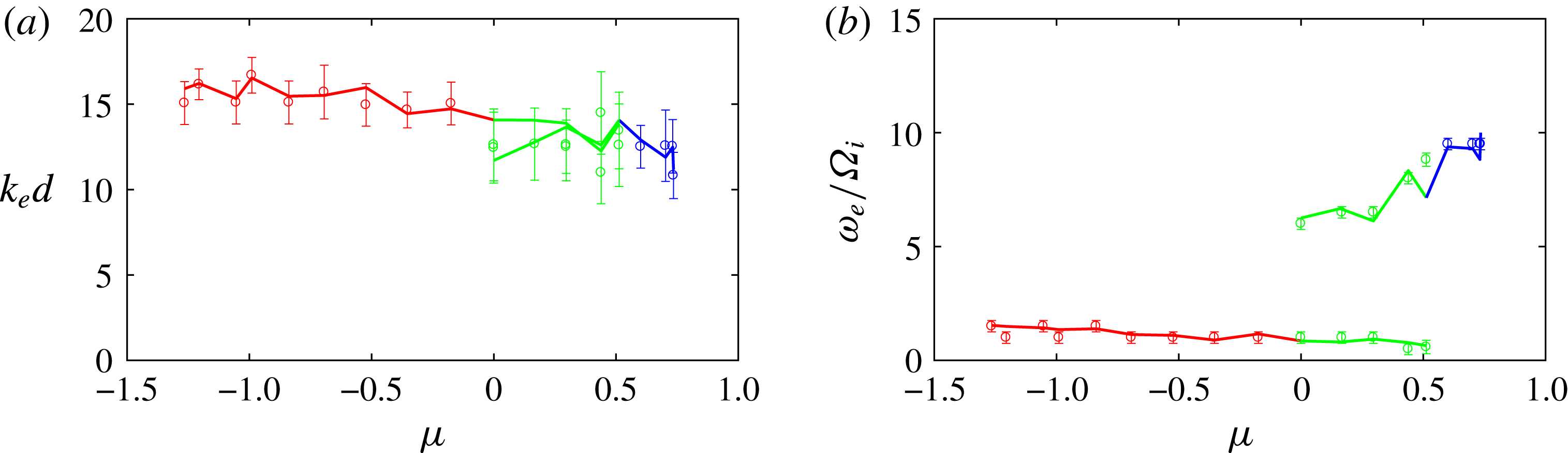
Comparison between the (a) axial wavenumber and (b) frequency obtained from the Fourier transform (empty circles with error bars) and obtained from direct measurements (lines) of the wavelength and period of some patterns in the spatio-temporal diagrams. The error bars are the same as in figure 14.

In the future, it would be interesting to study the effects of the gap ratio
 $\unicode[STIX]{x1D702}$
and the stratification
 $N$
to check these hypotheses. Besides, it would be of primary interest to further investigate the nonlinear dynamics of the primary and secondary instabilities and the subsequent transition to turbulence.
Acknowledgements
The first, third and fourth authors were supported by the Korea Meteorological Administration Research and Development Program under grant KMIPA 2015-5100 and KMIPA 2015-5190. The authors are grateful to three anonymous referees for providing valuable comments on this work. We also thank F. Gallaire and P. Monkewitz for giving us their set-up in order to perform preliminary experiments, and C. Frot and A. Garcia for their help.
Appendix. Measurements of axial wavenumber and frequency
Two methods have been used to retrieve the axial wavenumber and frequency of the primary modes from
 $z$
–
 $t$
spatio-temporal diagrams: a Fourier transform as explained in § 4 but also direct measurements of the mean wavelength and period of some patterns in the spatio-temporal diagrams. Figure 16 shows that the two methods give very similar results.