
1. Introduction
Trailing-edge noise is one of the dominant noise sources of aircraft, wind turbines and marine propellers (Lee et al. Reference Lee, Ayton, Bertagnolio, Moreau, Chong and Joseph2021; Moreau & Roger Reference Moreau and Roger2024). It is caused by the interaction between the turbulent boundary layer and the sharp trailing edge, having a broadband feature (Brooks, Pope & Marcolini Reference Brooks, Pope and Marcolini1989). The physical processes and theoretical models of trailing-edge noise have been described previously by Amiet (Reference Amiet1976) and Howe (Reference Howe1978) in their review papers. They found that the level of far-field noise is proportional to the wall-pressure fluctuation spectrum and the spanwise coherence length close to the trailing edge. Therefore, reducing the former properties by modifying the turbulent structures within the boundary layer could effectively attenuate the noise level. Bioinspired passive control techniques, such as trailing-edge separations (Chong & Joseph Reference Chong and Joseph2013; Avallone, Pröbsting & Ragni Reference Avallone, Pröbsting and Ragni2016; Liu, Zang & Azarpeyvand Reference Liu, Zang and Azarpeyvand2022) and porous materials (Geyer, Sarradj & Fritzsche Reference Geyer, Sarradj and Fritzsche2010; Ali, Azarpeyvand & Da Silva Reference Ali, Azarpeyvand and Da Silva2018; Feng & Ye Reference Feng and Ye2023), have been shown to be promising in noise mitigation. By influencing the noise source intensity and noise scattering process, a maximum noise reduction of around 10 dB has been achieved.
Inspired by the fine downy filaments over the owls’ wings, Clark et al. (Reference Clark, Baker, Alexander, Devenport, Glegg, Jaworski and Peake2016, Reference Clark, Alexander, Devenport, Glegg, Jaworski, Daly and Peake2017) proposed a novel biomimetic approach. They installed a spanwise array of thin and elongated finlets close to the trailing edge, oriented in the streamwise direction. Using the finlet treatment around the trailing edge of a DU96-W180 airfoil at a chord-based Reynolds number ( ${\textit {Re}}_c = U_\infty c/\nu$, where
 $U_\infty$ is the free-stream velocity,
 $c$ is the chord length of the airfoil and
 $\nu$ is the kinematic viscosity) of
 $3 \times 10^5$, Clark et al. (Reference Clark, Alexander, Devenport, Glegg, Jaworski, Daly and Peake2017) successfully achieved up to 10 dB of broadband noise attenuation in a wide range of angle of attack (
 $0^\circ$–
 $9^\circ$). The wall-pressure fluctuations were reduced in mid- and high-frequency ranges and increased in the low-frequency range. They conjectured that the mechanisms of noise reduction are not through affecting the noise scattering efficiency, but by modifying the boundary layer properties and flow structures. In addition, the influence on the aerodynamic performance is relatively small, with a similar lift and a slight increase in drag due to the larger area of the wetted surface in comparison with the untreated airfoil. A similar noise reduction effect was also obtained in other research (Millican et al. Reference Millican, Clark, Devenport and Alexander2017; Gstrein et al. Reference Gstrein, Zang, Mayer and Azarpeyvand2021b, Reference Gstrein, Zang, Mayer and Azarpeyvand2022; Fiscaletti et al. Reference Fiscaletti, Luesutthiviboon, Avallone and Casalino2022; Palani et al. Reference Palani, Paruchuri, Joseph, Karabasov, Utyuzhnikov, Devenport and Glegg2022).
Although revealing noise reduction potential, the mechanisms related to the modification of the turbulent boundary layer need to be further investigated. Afshari et al. (Reference Afshari, Azarpeyvand, Dehghan, Szőke and Maryami2019) studied the flow field downstream of the finlets over a flat plate experimentally using hotwire anemometry and surface pressure transducers. They found that the spanwise spacing between the finlets strongly influenced the mean flow topology and wall-pressure fluctuations. A decrease in the wall-pressure fluctuation spectrum in mid- and high-frequency ranges was observed. They proposed that the reduction is related to the increase of energy dissipation through surface friction of the finlet walls (referred to as the ‘channelling effect’). However, a separated shear layer was found to develop downstream of the finlets, possibly leading to the enhancement of wall-pressure fluctuations in the low-frequency band. Bodling & Sharma (Reference Bodling and Sharma2019) performed wall-resolved large eddy simulations with finlets being applied directly at the trailing edge of a NACA0012 airfoil at  ${\textit {Re}}_c = 5\times 10^5$. Similar wall-pressure fluctuation spectra were obtained. The finlets cause a redistribution of the turbulent kinetic energy in the boundary layer, resulting in an increase in the energy level directly above the finlets. On the other hand, the near-wall energy level between the finlets decreases. They referred to the scenario as the ‘lifting effect’, since the velocity fluctuation maxima are located away from the wall compared with the untreated case. They proposed that the increase in the spatial distance between the coherent structures and trailing edge leads to the attenuation of the noise scattering efficiency.
However, the contribution of channelling and lifting effects to noise reduction remains controversial. Palani et al. (Reference Palani, Paruchuri, Joseph, Karabasov, Utyuzhnikov, Devenport and Glegg2022) analysed the flow field around the finlet treatments at the trailing edge of a NACA0012 airfoil using hotwire anemometry. Different from Bodling & Sharma (Reference Bodling and Sharma2019), they observed that the local separation generated atop the finlets is responsible for the increase of turbulent fluctuations, rather than the lifting of the turbulent structures. Gstrein, Zang & Azarpeyvand (Reference Gstrein, Zang and Azarpeyvand2023) extended the experimental research of Afshari et al. (Reference Afshari, Azarpeyvand, Dehghan, Szőke and Maryami2019), analysing the pressure–velocity correlation within and close to the finlets using similar measurement techniques. The boundary layer profiles indicate the possible generation of turbulent structures on top of the finlets, which will convect downstream and remain separated from the airfoil surface. They explained that the mixing and merging between the turbulent structures shed above the finlets with the turbulent-channelled flow through the finlets could significantly attenuate the near-wall turbulent intensity and pressure fluctuations due to increased viscous friction. On the other hand, the lifting effect was considered to be less significant.
Most previous research has been focused on the statistical analyses of pressure fluctuation spectra and pressure–velocity correlations with the application of Taylor's hypothesis. Detailed analysis of the instantaneous flow organisation and their relation with pressure and noise is necessary to consolidate the understanding of finlet-induced noise reduction. Shi & Kollmann (Reference Shi and Kollmann2021) used wall-modelled large-eddy simulations with finlet treatments installed on a NACA0012 airfoil. They reported that the finlets increase the bluntness of the trailing edge, resulting in the formation of large-scale vortices shed from the blunt trailing edge. Similarly, by using overset large-eddy simulation, Ananthan & Akkermans (Reference Ananthan and Akkermans2023) observed the formation of a stream of hairpin-like vortices from the finlets, which convect downstream following a lifting-up process. No mixing or interaction with the channelled flow was detected, which is considered the key reason for the noise reduction in the mid and high frequencies. To the best of the authors’ knowledge, experimental research on the turbulent coherent structures induced by the finlets has not yet been reported.
The relationship between turbulent coherent structures of different scales with surface pressure fluctuations has been studied extensively for the zero-pressure gradient turbulent boundary layer over a flat plate. It has been recognised that the pattern of wall-pressure fluctuations is correlated with the turbulent events above it. By using direct numerical simulation, Kim (Reference Kim1983) applied the variable interval time-averaging (VITA) technique and found that the high-amplitude wall-pressure fluctuations are related to the streamwise inclined sweep events and turbulent bursting phenomenon. Thomas & Bull (Reference Thomas and Bull1983) further linked the bursting events to the shear layer that forms on the upstream side of large-scale hairpin-shaped vortices using the conditional averaging method and pointwise measurement. Ghaemi & Scarano (Reference Ghaemi and Scarano2013) focused on the high-amplitude pressure peaks (HAPPs) at the wall and the related turbulent structures. Using tomographic particle image velocimetry (PIV), they revealed that the positive HAPPs are related to the stagnation point of shear layer structures resulting from an upstream sweep event, followed by a downstream ejection event caused by hairpin vortices. The negative HAPPs are attributed to the spanwise and quasi-streamwise vortices. These results suggest that the hairpins are the major contributor to the wall-pressure fluctuations.
Moreover, the increase of adverse pressure gradient close to the trailing edge of the airfoil energies the large-scale structures in the outer region of the turbulent boundary layer, which is similar to the increase of Reynolds number (Harun et al. Reference Harun, Monty, Mathis and Marusic2013; Tanarro, Vinuesa & Schlatter Reference Tanarro, Vinuesa and Schlatter2020). For the high-Reynolds-number condition, Naka et al. (Reference Naka, Stanislas, Foucaut, Coudert, Laval and Obi2015) used the pressure–velocity correlation technique and found that the positive and negative pressure fluctuations are related to the hairpin-shaped coherent structures, similar to those identified by Ghaemi & Scarano (Reference Ghaemi and Scarano2013). They also pointed out that the intense and fast variations of the wall-normal velocity are strongly correlated with the wall-pressure fluctuations. In addition, they noted a weak correlation region of elongated shape attached to the wall, indicating the link to the very-large-scale motions (VLSMs) (Hutchins & Marusic Reference Hutchins and Marusic2007; Lee et al. Reference Lee, Lee, Choi and Sung2014). Gibeau & Ghaemi (Reference Gibeau and Ghaemi2021) filtered the pressure signal into large-scale and very-large-scale components and analysed the related coherent structures by frequency-dependent pressure–velocity coherence method. They found that both VLSMs and hairpin vortices contribute to the production of wall-pressure fluctuations. The VLSMs produce positive and negative wall-pressure fluctuations by inducing splitting and lifting motions.
The effect of finlet treatments on the turbulent structures of different scales has not been addressed before, which is closely related to the wall-pressure pattern and the possible generation of far-field noise. The present investigation aims to understand the underlying mechanisms of pressure and noise reduction effect by the finlet treatments, specifically focusing on the modification of turbulent structures close to the trailing edge of a NACA0018 airfoil. The far-field noise and pressure fluctuation reduction capability of finlets with different spacing are analysed. The unsteady flow features are identified using time-resolved PIV. Two streamwise planes coinciding with the finlet and between the finlets are measured, elucidating both the finlet-induced structures and the modification of the channelled flow through the finlets. The relation between pressure fluctuations and turbulent structures of different scales is obtained by pressure–velocity coherence and correlation. The coherent structures responsible for the production of HAPPs are returned by conditional averaging, highlighting the importance of the generation and modification of turbulent structures by the finlet treatments.
2. Experimental set-up and flow conditions
2.1. Flow facility and finlet configurations
The experiments were performed in an open-jet low-speed anechoic wind tunnel at the Institute of Fluid Engineering, Zhejiang University. The test section of the wind tunnel is 500 mm in width and 400 mm in height. The maximum incoming velocity is  $60\,{\rm m}\,{\rm s}^{-1}$ with a well-controlled turbulent intensity of below
 $0.5\,\%$. The cut-off frequency of the wind tunnel is 170 Hz.
An aluminium NACA0018 airfoil was installed at the centre plane of the test section as shown in figure 1(a). The airfoil has a chord length of  $c = 200$ mm and a span of
 $l = 400$ mm. A zig-zag stripe (figure 1b) was installed at 8 mm downstream of the leading edge to achieve a fully developed turbulent condition before reaching the finlet treatment. The thickness and the width of the zig-zag stripe are 0.8 mm and 9 mm, respectively. A Cartesian coordinate system with the origin located at the spanwise centre of the trailing edge is introduced. The
 $y$- and
 $z$-axes represent the wall-normal and spanwise directions, respectively. The
 $x$-axis is normal to the former axes to form a right-handed reference system, being parallel to the airfoil surface.
Conceptual sketch of model installation and experimental set-up: (a) model installation; (b) NACA0018 airfoil with finlet treatment; (c) finlet design and geometric parameters.

The finlet treatments are placed 20 mm upstream of the trailing edge for both sides of the airfoil, extending over the entire span. The shape of the finlets is designed following Afshari et al. (Reference Afshari, Azarpeyvand, Dehghan, Szőke and Maryami2019) and Gstrein et al. (Reference Gstrein, Zang, Mayer and Azarpeyvand2022, Reference Gstrein, Zang and Azarpeyvand2023) as shown in figure 1(c). They consist of a series of vertical finlets oriented in the streamwise direction with a substrate layer. The thickness of the finlets and the substrate layer is 0.5 mm. A local Cartesian coordinate is introduced with the origin ( $o_F$) located at the rear of the finlets. The directions of
 $x_F$,
 $y_F$ and
 $z_F$ follow that of the airfoil coordinate system. The leading-edge profile of the finlets is shaped as
 \begin{equation} \eta(x_F) = 0.65\times (x_{F}+40)^{0.8}, \end{equation}
where  $\eta (x_{F})$ is the wall-normal distance from the airfoil surface. The streamwise length of the finlet (
 $L$) is 40 mm. The maximum height from the substrate is 6 mm, which is about 60 % of the boundary layer thickness
 $\delta _{99}$ (the wall-normal location at which the local time-averaged streamwise velocity
 $U = 0.99U_\infty$) at
 $x/c = 0.99$ for the untreated case, aligning with the optimised ratio for noise reduction as reported by Gstrein et al. (Reference Gstrein, Zang, Mayer and Azarpeyvand2022, Reference Gstrein, Zang and Azarpeyvand2023). The overall maximum height (
 $H$) is 6.5 mm. The backside of the finlets is rounded with a radius (
 $r$) of 6.5 mm. The shape is expected to reduce finlet self-noise (Gstrein et al. Reference Gstrein, Zang and Azarpeyvand2023). Three spanwise spacings (
 $S$) between neighbouring finlets are investigated, including
 $S = 12$ mm, 6 mm and 3 mm (referred to as S12, S6 and S3, respectively). The substrate layer of the finlets is well attached to the surface due to the small curvature of the airfoil close to the trailing edge.
The geometric angle of attack of the airfoil was kept constant at  $\alpha _{geo} = 0^\circ$. To obtain the effective angle of attack (
 $\alpha _{eff}$), the static pressure was measured over both sides of the airfoil by the pressure scanning valve (Hanghua PSU32) in the range of
 $x/c = [-0.72, -0.36]$. Over each side of the airfoil, ten pressure taps are aligned with an angle of
 $30^\circ$ with respect to the chord to avoid interference between neighbouring sensors. The measurements were performed with a sampling frequency of 500 Hz and a duration of 10 s. The pressure coefficient (
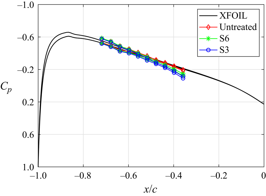
 $C_p$) distribution of the untreated, S6 and S3 cases are compared with the prediction obtained from XFOIL, as shown in figure 2. Good agreement is obtained with the predicted result of
 $0.2^\circ$, confirming the effective angle of attack (
 $\alpha _{eff}$) in the current experiment. Compared with the untreated case, the finlet treatments (S6 and S3) lead to an increase of
 $C_p$ in its close vicinity (
 $x/c = [-0.3, -0.1]$), which is due to the resistance to the flow by the finlet leading edges (Farabee & Casarella Reference Farabee and Casarella1984; Leclercq et al. Reference Leclercq, Jacob, Louisot and Talotte2001).
Pressure coefficient distribution ( $C_p$) of the untreated, S6 and S3 cases, compared with the predicted result from XFOIL at
 $\alpha _{eff} = 0.2^\circ$.

2.2. Experimental set-up
2.2.1. Far-field noise measurement
The far-field noise was recorded by a GRAS 40PH-10 CCP free-field microphone, which has a frequency response of  $\pm$2 dB. The microphone works in a frequency range from 10 Hz to 20 kHz with a maximum output of 135 dB ref.
 $20 \,\mathrm {\mu }\mathrm {Pa}$. The microphone was mounted at a distance of 1 m from the spanwise centre of the airfoil trailing edge, with an azimuthal angle of
 $90^\circ$. The data were sampled using a National Instruments PXIe-4499 with a frequency of 50 kHz for 30 s. The sound pressure level (SPL) is calculated as
 $\mathrm {SPL}=20\log _{10}{(p_{rms}^\prime /p_0)}$, where
 $p_{rms}^\prime$ designates the root mean square of the sound pressure fluctuations,
 $p_0$ is the reference pressure which equals
 $20\,\mathrm {\mu }\mathrm {Pa}$. The overall sound pressure level (OASPL) is obtained by integrating the energy spectrum with respect to frequency using
 $\mathrm {OASPL}=10\log _{10}[{\int \operatorname {S}(f) \,\mathrm {d} f}/{p_{0}^2}]$, where
 $S(f)$ is the power spectral density (PSD) based on the sound pressure fluctuations.
2.2.2. Unsteady wall-pressure fluctuation measurement
The unsteady wall-pressure fluctuations ( $p^\prime$) were measured using seven FG-23329-P07 pressure transducers, with a frequency response of
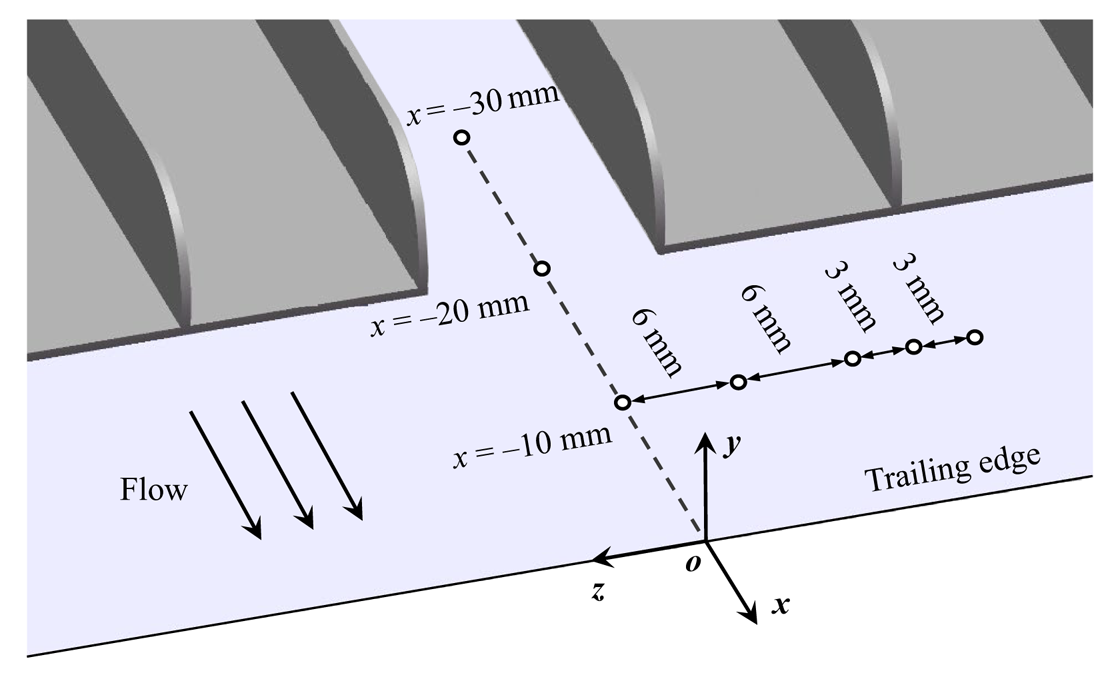
 $\pm$3 dB and a frequency range of 100 Hz to 10 kHz. The transducers were mounted beneath a pinhole of 0.4 mm diameter to avoid pressure attenuation at high frequencies (Garcia-Sagrado, Hynes & Hodson Reference Garcia-Sagrado, Hynes and Hodson2006; Showkat Ali et al. Reference Showkat Ali, Azarpeyvand, Szőke and Ilário da Silva2018), as shown in figure 3. Three pressure transducers were installed at the spanwise symmetry plane (
 $z = 0$ mm), with the corresponding streamwise locations of
 $x = -10$ mm,
 $-20$ mm and
 $-30$ mm, respectively. When measuring the wall-pressure fluctuations within the region of finlet treatments (
 $x = -30$ mm), part of the substrate layer was removed. The influence of this action on the flow field and wall pressure is negligible as the substrate layer is very thin. In addition, due to the importance of the spanwise coherence length to the trailing-edge noise (Amiet Reference Amiet1976), five transducers are placed along the span at
 $x = -10$ mm (95 % chord length). The spanwise spacings between neighbouring transducers are 6 mm, 6 mm, 3 mm and 3 mm, respectively. The pressure transducers were calibrated against a GRAS 40PH-10 CCP far-field microphone similar to the previous studies (Showkat Ali et al. Reference Showkat Ali, Azarpeyvand, Szőke and Ilário da Silva2018; Afshari et al. Reference Afshari, Azarpeyvand, Dehghan, Szőke and Maryami2019), resulting in the sensitivity varying approximately between 20 and
 $25\,{\rm mV}\,{\rm Pa}^{-1}$. The measurements were performed with a sampling frequency of 48 000 Hz and a duration of 10 s.
The distribution of the surface pressure transducers.

2.2.3. Time-resolved PIV
The time-resolved planar PIV measurements were performed to capture the instantaneous velocity field of the turbulent boundary layer with and without finlet treatments. A high-speed CMOS camera (Photron FASTCAM Mini AX100,  $1024 \times 1024$ pixels,
 $20\,\mathrm {\mu }\mathrm {m}\,{\rm pixel}^{-1}$) was applied to capture the particle images, which was equipped with an objective of 105 mm focal length. The aperture of this camera was set at
 $f_\# = 4$. The flow was seeded with water–oil droplets of approximately
 $1\,\mathrm {\mu }\mathrm {m}$ diameter. The tracer particles were illuminated by a laser sheet of about 1 mm thickness, being produced by the Nd:YLF high-speed laser (527 nm, Beamtech Vlite-Hi-527-50,
 $50\,{\rm mJ}\,{\rm pulse}^{-1}$ at 1 kHz). The field of view (FOV) is
 $53 \times 16\,{\rm mm}^{2}$ (
 $x \times y$), which covers the streamwise range of
 $x = [-40, 13]$ mm and extends from the finlets area to the wake of the airfoil. The digital image resolution is
 $19.3\,{\rm pixels}\,{\rm mm}^{-1}$. The pulse separation was set to
 $25\,\mathrm {\mu }\mathrm {s}$. The snapshots were acquired at 6000 Hz with an ensemble data size of 12 000. The raw images were pre-processed with background subtraction, intensity normalisation, and Gaussian smoothing in LaVision DaVis 10. The velocity field is evaluated by a multipass cross-correlation method with window deformation. The final interrogation window size is
 $16 \times 16\,{\rm pixel}^{2}$ with an overlap of 75 %, resulting in a vector pitch of 0.21 mm.
To obtain the correlation and coherence between the unsteady flow structures and the wall-pressure fluctuations, the PIV measurement plane coincides with the surface pressure transducers aligning in the streamwise direction. The spanwise variation of the flow field was captured by placing the finlets at two spanwise locations: one with the PIV measurement plane coinciding with the finlet (referred to as the ‘finlet plane’, as shown in figure 4b); for the other, the PIV measurement plane is located between two neighbouring finlets (referred to as the ‘mid plane’, as shown in figure 4c). Using the local Cartesian coordinate, the finlet plane and mid plane correspond to the spanwise location of  $z_{F}/S = 0$ and
 $z_{F}/S = 0.5$, respectively. Moreover, the velocity fields and surface pressure fluctuations were measured simultaneously, being synchronised by the National Instruments PXIe-4499 and an inhouse LabView control program.
Conceptual sketch of the planar PIV set-up: (a) perspective view; (b) finlet plane; (c) mid plane.

2.3. Turbulent boundary layer properties
The free-stream velocity was kept constant at  $U_\infty = 20\,{\rm m}\,{\rm s}^{-1}$ in the experiment campaigns. The resultant chord-based Reynolds number (
 ${\textit {Re}}_c$) is
 $2.7 \times 10^5$. Due to the rapid development of the boundary layer under adverse pressure gradient, the results of the properties vary significantly spatially (Garcia-Sagrado et al. Reference Garcia-Sagrado, Hynes and Hodson2006; Ghaemi & Scarano Reference Ghaemi and Scarano2011). Two streamwise positions at
 $x = -10$ mm and
 $-20$ mm are selected to estimate the boundary layer properties for the untreated case, corresponding to 95 % and 90 % of the chord length, respectively. The boundary layer thickness
 $\delta _{99}$, displacement thickness (
 $\delta ^\ast$), momentum thickness (
 $\theta$), friction velocity (
 $u_\tau$), shape factor (
 $H_{12}$), Reynolds number based on the momentum thickness (
 ${\textit {Re}}_\theta =U_\infty \theta /\nu$) and friction velocity (
 ${\textit {Re}}_\tau =u_\tau \delta _{99}/\nu$) are summarised in table 1. The friction velocity (
 $u_\tau =\sqrt {1/2 U_\infty ^2 c_f }$) is determined by the estimation of the friction coefficient (
 $c_f$) following the interpolation method proposed by Allen & Tudor (Reference Allen and Tudor1969). The pressure gradient at
 $x = -20$ mm is estimated by the calculation from XFOIL for the untreated case, resulting in the Clauser's equilibrium parameter
 $\beta _{c}$ of 3.2 (
 $\beta _{c}= (\theta /\tau _{w})/({\rm d}p/{{\rm d}\kern0.7pt x})$, where
 $\tau _{w}$ is the surface skin friction) (Clauser Reference Clauser1954). Due to the influence of the adverse pressure gradient close to the trailing edge, the shape factors (
 $H_{12}$) are much higher than that of the zero-pressure gradient condition, especially for the positions of
 $x = -10$ mm, which agrees with the experiment of Ghaemi & Scarano (Reference Ghaemi and Scarano2011).
Summary of the turbulent boundary layer properties.

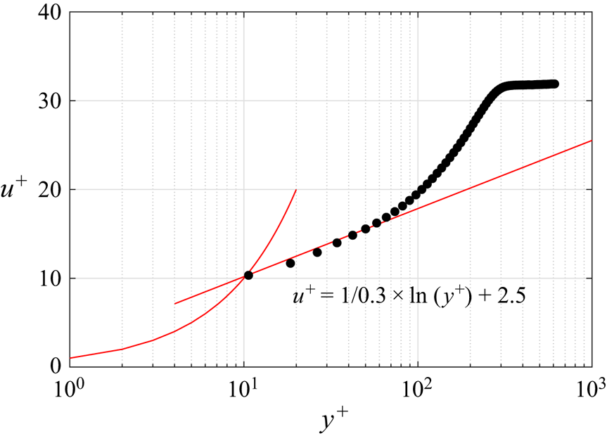
To validate the fully turbulent condition close to the trailing edge, the logarithmic boundary layer profile of the untreated airfoil at  $x = -20$ mm is shown in figure 5. It is worth noting that the non-equilibrium of the boundary layer near the trailing edge leads to a higher slope of the logarithmic layer compared with the zero-pressure gradient condition, as described by Garcia-Sagrado et al. (Reference Garcia-Sagrado, Hynes and Hodson2006). The mean velocity profile agrees well with the logarithmic law with
 $\kappa = 0.3$ and
 $B = 2.5$, as illustrated in figure 5.
Logarithmic profile of the time-averaged streamwise velocity for the untreated airfoil at  $x = -20$ mm. The red line represents the log-law fit. Here
 $u^+ = U/u_\tau$ and
 $y^+ = yu_\tau /\nu$.

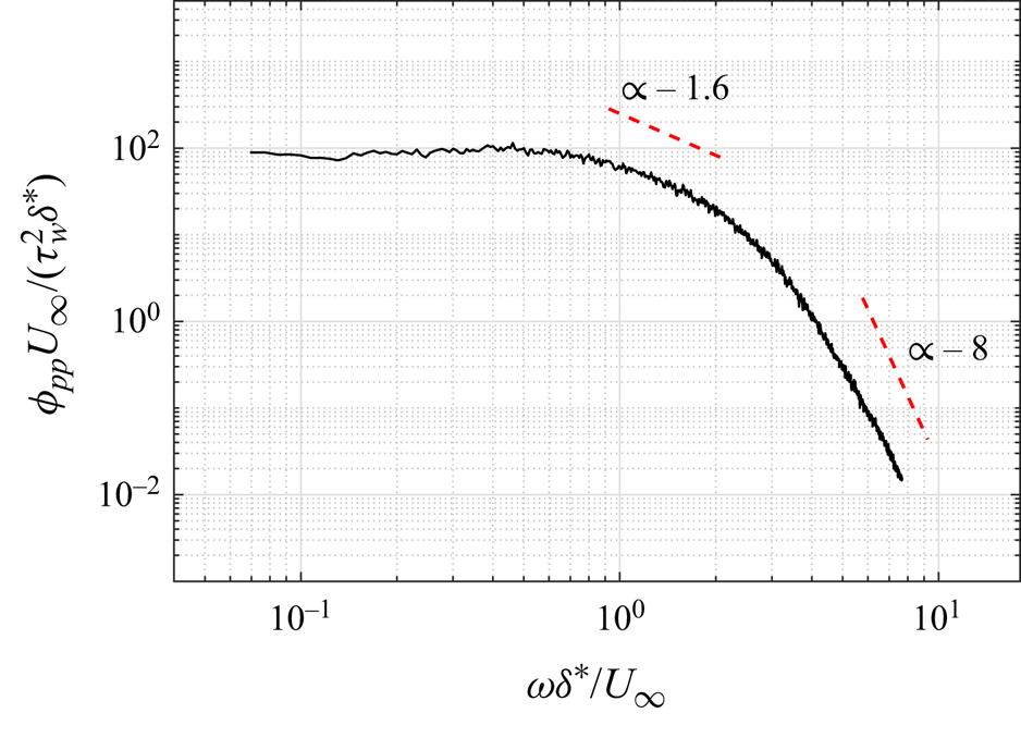
The PSD of the wall-pressure fluctuations ( $\phi _{pp}$) of the untreated case at
 $x = -20$ mm is displayed in figure 6, which is scaled as
 $\phi _{pp}U_{\infty }/(\tau ^{2}_{w}\delta ^{*})$ and plotted against
 $\omega \delta ^{*}/U_{\infty }$, where
 $\omega$ is the angular frequency (
 $\omega = 2{\rm \pi} f$). Different from the empirical wall-pressure spectral modelling for zero-pressure-gradient flows (Goody Reference Goody2004; Hwang, Bonness & Hambric Reference Hwang, Bonness and Hambric2009), the presence of an adverse pressure gradient leads to a faster decay of the wall-pressure spectrum, especially for the low-Reynolds-number flows (Rozenberg, Robert & Moreau Reference Rozenberg, Robert and Moreau2012). The decay rates of the spectrum are
 $\omega ^{-1.6}$ and
 $\omega ^{-8}$ in the range of
 $0.9<\omega \delta ^{*}/U_{\infty }<2$ and
 $\omega \delta ^{*}/U_{\infty }>4$, respectively, agreeing with the results of the empirical wall-pressure spectrum model developed by Lee (Reference Lee2018). This correspondence provides validation for the accuracy of the current wall-pressure fluctuation measurements.
The scaled PSD of the wall-pressure fluctuations at  $x = -20$ mm for the untreated airfoil.

3. Far-field noise
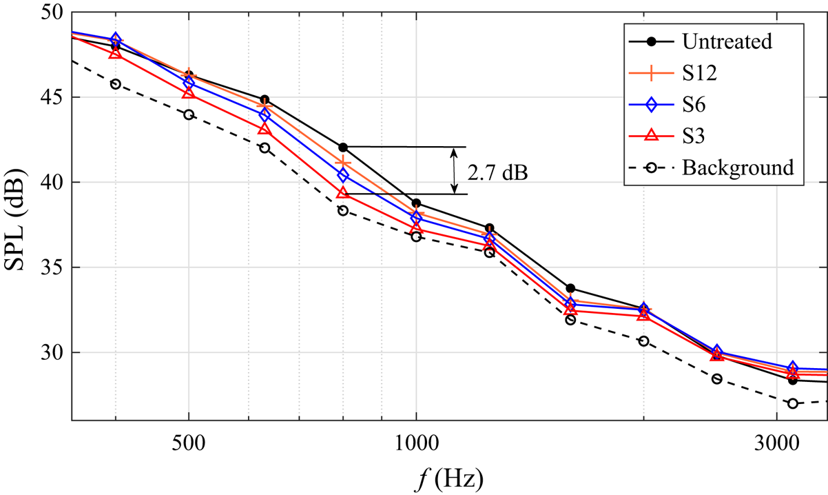
The effect of finlets of three spanwise spacings (S3, S6 and S12) on trailing-edge noise is investigated first. The far-field noise (SPL) is calculated with the 1/3-octave band, as presented in figure 7. The cases of the untreated airfoil and background noise of the wind tunnel are plotted for comparison. Noise reduction in the frequency range of 400–2000 Hz is obtained for all three finlet configurations. The smaller spanwise spacing finlets lead to a stronger noise reduction effect, with the S3 treatment leading to a maximum decrease of 2.7 dB at around 800 Hz. It should be noted that due to the maximum SPL difference is 3.7 dB between the untreated case and the background noise, the current results may underestimate the noise reduction capability of the finlet treatments. The difference in OASPL ( $\Delta$OASPL) between the finlet and the untreated cases is presented in table 2. The integration is performed in the range of noise reduction frequency band (400–2000 Hz), using the A-weighting function. Larger
 $\Delta \,{\rm OASPL}$ is achieved with smaller spacing finlets.
Far-field SPL in the 1/3-octave band for different finlet configurations, compared with the untreated airfoil and background noise of the wind tunnel.

OASPL difference ( $\Delta \,{\rm OASPL}$) between the finlet-treated cases and the untreated case, being assessed using A-weighting.

4. Unsteady wall-pressure fluctuations
According to the Amiet model (Amiet Reference Amiet1976), the far-field trailing-edge noise is proportional to the wall-pressure fluctuation spectrum and spanwise coherence length. The streamwise evolution of the wall-pressure fluctuation PSD with finlet treatments is presented in figure 8 for the S6 and S3 cases at the mid planes (S6-M and S3-M), as the two spacings finlets lead to a stronger noise reduction effect. The result of the untreated case is plotted for comparison. Both treated cases show a decrease in the mid- and high-frequency ranges compared with the untreated case for all the streamwise locations. The finlets with smaller spacing cause a more pronounced reduction, which is similar to the previous research (Afshari et al. Reference Afshari, Azarpeyvand, Dehghan, Szőke and Maryami2019; Gstrein et al. Reference Gstrein, Zang, Mayer and Azarpeyvand2022, Reference Gstrein, Zang and Azarpeyvand2023). The suppression intensifies significantly when moving downstream of the finlet treatment area (figure 8c), attributing to the upward movement and disruption of near-wall turbulent structures. At low frequencies, the magnitude of the PSD increases, which is associated with the generation of large-scale structures induced by the finlets. This scenario was also confirmed by Ananthan & Akkermans (Reference Ananthan and Akkermans2023), who found that the finlets produce a train of hairpin-like vortices originating from the front part of the finlets.
The PSD of wall-pressure fluctuations at three streamwise locations for the finlet and untreated configurations: (a)  $x/H = -4.62$; (b)
 $x/H = -3.08$; (c)
 $x/H = -1.54$.

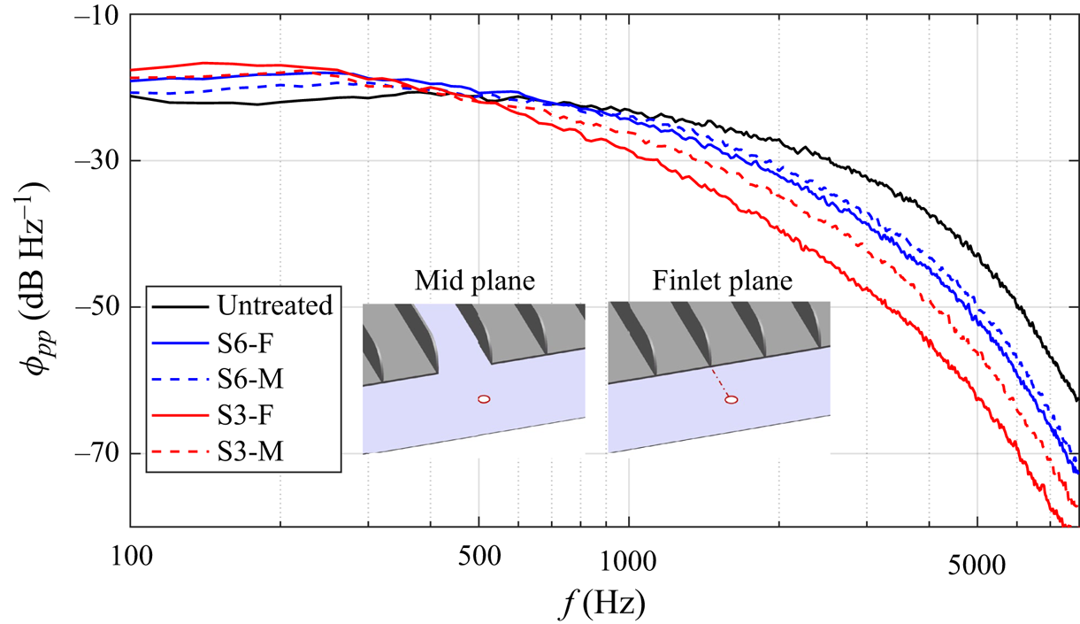
The variations of the wall-pressure fluctuations in the spanwise direction are analysed in the wake of the finlets ( $x/H = -1.54$), as shown in figure 9. The PSD yields a similar overall trend for both the finlet (S3-F and S6-F) and mid planes (S3-M and S6-M). A more pronounced reduction of PSD magnitude at high frequencies and an increase at low frequencies are produced at the finlet plane. The former effects intensify with the decrease of spanwise spacing. The frequency range of magnitude change agrees with that of the far-field noise. As a result, it is inferred that the suppression of wall-pressure fluctuations in the mid- and high-frequency ranges is the major contributor to the noise reduction effect induced by finlets. One can find that above 2000 Hz, the SPL (see figure 7) does not show magnitude reduction as obtained for the wall-pressure fluctuations, which is associated with the high-frequency finlet self-noise induced by the interaction between the finlets and the flow (Gstrein, Zang & Azarpeyvand Reference Gstrein, Zang and Azarpeyvand2021a).
Spanwise variation of wall-pressure fluctuation spectrum at  $x/H = -1.54$ for the finlet and untreated configurations.

The spanwise turbulent coherence length scale ( $\varLambda _z$) is calculated by the wall-pressure fluctuations, following the estimation approach proposed by Roger, Moreau & Guédel (Reference Roger, Moreau and Guédel2006) as
 \begin{equation} \gamma^{2}(\,f, \Delta z)=\frac{\left|\phi_{p p}(f, \Delta z)\right|^{2}}{\phi_{p p}^{2}(f)} \approx e^{-\Delta z^{2} / \varLambda_{z}^{2}}, \end{equation}
where  $\gamma$ is the spanwise coherence of wall-pressure fluctuations and
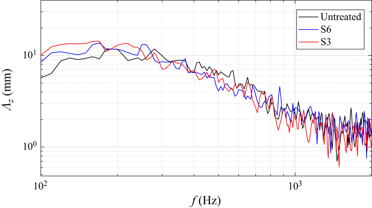
 $\Delta z$ is the spanwise step. Figure 10 illustrates the spanwise coherence length scale of the untreated, S6 and S3 cases. Both the S6 and S3 cases cause an increase of the length scale below 250 Hz compared with the untreated case. However, when the frequency exceeds 300 Hz, the coherence length tends to collapse for all the cases. As a result, the spanwise coherence length does not directly correlate with the noise reduction effect induced by the finlets in the current experiment.
Spanwise coherence length scale at  $x/H = -1.54$ for the finlet and untreated configurations.

5. Time-averaged flow field and turbulent statistics
To further understand the mechanisms related to the noise and pressure fluctuation suppression, the modification of the turbulent boundary layer by finlet treatments is firstly analysed by the normalised time-averaged streamwise velocity ( $U/U_\infty$) and Reynolds shear stress (
 $-\overline {u^{\prime } v^{\prime }} / U_{\infty }^2$,
 $u^{\prime }$ and
 $v^{\prime }$ are the streamwise and wall-normal velocity fluctuations, respectively). The
 $x\unicode{x2013}y$ cross-plane contour with different finlet treatments is shown in figures 11 and 12 for the finlet and mid planes, respectively. The streamlines are superimposed for clarity. The streamwise evolution of maximum shear stress is shown by the dashed lines.
Contours of time-averaged streamwise velocity ( $U/U_\infty$) and Reynolds shear stress (
 $-\overline {u^{\prime } v^{\prime }} / U_{\infty }^2$) for the untreated and treated cases at the finlet plane: (a,b) untreated case, (c,d) S6-F case and (e,f) S3-F case. The yellow and green dashed lines indicate the streamwise evolution of detached and near-wall shear layers. The red cross symbol represents the reattachment point.

Contours of time-averaged streamwise velocity ( $U/U_\infty$) and Reynolds shear stress (
 $-\overline {u^{\prime } v^{\prime }} / U_{\infty }^2$) for the treated cases at the mid plane: (a,b) S6-M case; (c,d) S3-M case.

For the streamwise velocity at the finlet planes (figure 11c,e), momentum transport and redistribution of the shear stress are induced along the wall-normal direction for both the S6 and S3 cases. As a result, a detached shear layer forms on top of the finlets (yellow dashed lines, figure 11d,f), originating from  $x/H = -5$,
 $y/H = 1$. The shear layer undergoes an upward movement due to the induced upwash motion (Hwang & Lee Reference Hwang and Lee2018; Medjnoun, Vanderwel & Ganapathisubramani Reference Medjnoun, Vanderwel and Ganapathisubramani2020). The former region is prone to the growth of shear layer instability, leading to the generation of hairpin vortices (Ye, Schrijer & Scarano Reference Ye, Schrijer and Scarano2016, Reference Ye, Schrijer and Scarano2018). The increase of Reynolds shear stress leads to the intensified momentum exchange, which further modifies the distribution of coherent structures in the boundary layer. Meanwhile, a narrow region of negative shear stress appears below the detached shear layer behind the finlets, which is similar to the secondary phenomena of the flow past a circular cylinder (Bouard & Coutanceau Reference Bouard and Coutanceau1980). Considering the effect of spanwise spacing, it is worth noting that the magnitude of Reynolds shear stress is relatively small for the S3 case, being attributed to the more intensive viscous diffusion and faster breakdown process of unsteady vortical structures (Ye et al. Reference Ye, Schrijer and Scarano2016, Reference Ye, Schrijer and Scarano2018).
Close to the wall, a low-momentum region forms directly downstream of the finlets, where flow separation occurs (figure 11c,e). A larger separation bubble is produced by the finlets for smaller spanwise spacing, leading to a higher decrease in the near-wall streamwise velocity. The reattachment points (cross mark) of the separation bubble are located at  $x/H = -2.45$ and
 $-1.85$ for the S6-F and S3-F cases, respectively. Near-wall high-shear layers are produced on top of the separation bubble, evolving downstream with an upward inclination of
 $7.5^\circ$ and
 $8.5^\circ$ with respect to the airfoil surface (
 $x/H \leq 0$) for the S6-F and S3-F cases, respectively (see the green dashed lines in figure 11d,f). The overall lift-up process is attributed to the mutual interaction between the detached and near-wall shear layers, leading to the reduction of near-wall shear stress until the airfoil trailing edge. The flow separation and induced near-wall shear layer are expected to contribute to the formation of the spanwise vortices (Burgmann & Schröder Reference Burgmann and Schröder2008).
On the other hand, for the mid planes, the results vary significantly with the change of spanwise spacings. For the case of larger spanwise spacing (S6-M), the flow field tends to return to the untreated turbulent boundary layer condition, indicating that the influenced area is confined close to the finlets. However, the velocity decreases close to the wall is still observed, as shown in figure 12(a,b). While for the S3-M case, the overall distribution of the flow topology and Reynolds shear stress resembles that at the finlet plane (S3-F). The detached and near-wall shear layer preserves with reduced intensity due to the smaller spacing between adjacent finlets. It is conjectured that the finlets with smaller spacing enable full coverage of momentum transport over the airfoil span, which leads to a more pronounced reduction in far-field noise and wall-pressure fluctuations (see figures 7 and 9).
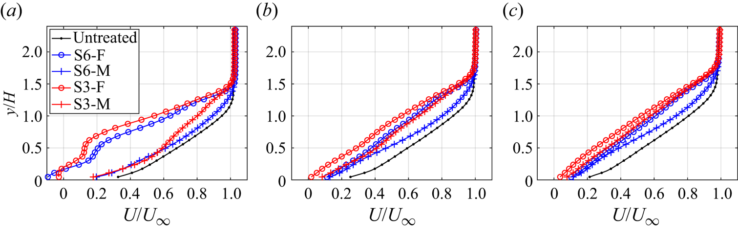
The momentum modification is quantitatively compared by extracting the boundary layer profiles of the streamwise velocity at  $x/H = -3.0$,
 $-1.5$ and
 $-0.5$, as shown in figure 13. Close to the rear of the finlets at
 $x/H = -3$ (figure 13a), a significant overall velocity decrease is observed at the finlet planes (S6-F and S3-F) with respect to the untreated case due to the induced upwash motion (
 $\kern 1.5pt y/H = [0.35, 1.0]$) and backward separation (
 $\kern 1.5pt y/H < 0.35$). The velocity deficit increases with the decrease of spanwise spacing of the finlets. The maximum velocity deficit of
 $0.55U_\infty$ and
 $0.60U_\infty$ is produced at
 $y/H = 0.6$ for S6-F and S3-F, respectively. The emergence of an inflectional point appears at around
 $y/H = 1$, leading to the onset of local shear layer instability. Meanwhile, at the mid planes (S6-M and S3-M), the velocity deficit decreases significantly over the entire boundary layer. When moving downstream (figure 13b,c), the low-momentum region at the finlet planes undergoes a fast recovery process due to viscous diffusion and turbulent mixing (Sun et al. Reference Sun, Schrijer, Scarano and van Oudheusden2014; Ye et al. Reference Ye, Schrijer and Scarano2016). In contrast, the velocity deficit at the mid planes exhibits an opposite trend of evolution. As a result, the velocity difference between the two types of planes decreases at the downstream stages. An overall momentum reduction sustains to the trailing edge of the airfoil compared with the untreated case. Since the SPL caused by the edge scattering is proportional to the fifth power of the velocity of the convecting eddies (Bull Reference Bull1967), the notable velocity decrease contributes to the noise reduction, with the S3 finlet treatment being more effective due to the lower near-wall velocity. Shi & Lee (Reference Shi and Lee2020) and Ananthan & Akkermans (Reference Ananthan and Akkermans2023) also pointed out the importance of velocity decrease for noise reduction with finlet treatment.
Profiles of the time-averaged streamwise velocity ( $U/U_\infty$) at different streamwise locations for the untreated and treated cases: (a)
 $x/H = -3$; (b)
 $x/H = -1.5$; (c)
 $x/H = -0.5$.

The development of the velocity difference induced by the finlets is associated with the streamwise velocity gradient ( $\mathrm {d}(U/U_\infty )/\mathrm {d}(x/H)$), as shown in figure 14. The distributions for both finlet planes (figure 14a,c) feature a deceleration region at the detached shear layer and an acceleration region behind the finlets. Conversely, at the mid planes (figure 14b,d), an overall deceleration process is observed due to interaction between the channelled flow through the finlets and the finlet-induced structures, together with the presence of adverse pressure gradient close to the trailing edge. Maximum negative velocity gradient appears directly downstream of the finlets, which corresponds to the upwash motion and flow separation. After the fast deceleration, the streamwise velocity near the wall remains low and relatively constant, contributing to the trailing edge noise reduction (Bull Reference Bull1967).
Contours of streamwise velocity gradient in the streamwise direction ( $\mathrm {d}(U/U_\infty )/\mathrm {d}(x/H)$) at
 $x\unicode{x2013}y$ cross-plane: (a) S6-F case; (b) S6-M case; (c) S3-F case; (d) S3-M case.

6. Modulation of turbulent structures
6.1. Instantaneous flow field
To further understand the characteristics of the coherent structures induced by the finlet treatments, the instantaneous flow fields are illustrated by the normalised streamwise velocity ( $u/U_\infty$) and streamwise velocity fluctuations (
 $u^\prime /U_\infty$), as shown in figure 15. Only the S3 case is presented and compared with the untreated case for conciseness. The streamlines are superimposed for
 $u/U_\infty$ in figure 15(a,c,e). To better visualise the vortical structures produced at the detached shear layer, the selected streamlines shown in figure 15(d,f) (
 $u^\prime /U_\infty$) for the finlet cases are subtracted by the convection velocity of
 $0.75U_\infty$ and
 $0.06U_\infty$ in the streamwise and surface-normal directions, respectively (Adrian, Meinhart & Tomkins Reference Adrian, Meinhart and Tomkins2000). For the untreated case in figure 15(a,b), large-scale alternative low- and high-speed streaks form close to the wall, which inclines towards the downstream direction with an angle of approximately
 $15^\circ$. The velocity streaks correspond to the wall-attached structures, which are the dominant coherent structures and contribute significantly to the shear stress in the turbulent boundary layer (Abe Reference Abe2017; Yoon et al. Reference Yoon, Hwang, Yang and Sung2020). The corresponding movies (1 and 2) are provided in the supplementary material available at https://doi.org/10.1017/jfm.2024.1192 for better visualisation.
Contours of normalised instantaneous streamwise velocity ( $u/U_\infty$) and streamwise velocity fluctuations (
 $u^\prime /U_\infty$) at
 $x\unicode{x2013}y$ cross-plane: (a,b) untreated case; (c,d) S3-F case; (e,f) S3-M case.

With the implementation of the finlets, the instantaneous flow features are modified significantly. For the streamwise velocity at the finlet plane (figure 15c), the detached shear layer over the finlets and the induced upwash motion lead to the generation of unstable wavy motions due to local inflectional instability at the turbulent non-turbulent interface, causing the increase of the boundary layer thickness (Afshari et al. Reference Afshari, Azarpeyvand, Dehghan, Szőke and Maryami2019; Ananthan & Akkermans Reference Ananthan and Akkermans2023). Close to the wall ( $\kern 1.5pt y/H < 0.5$), strong flow separation emerges (
 $x/H = [-3, 0]$), leading to the formation of the spanwise vortices and the near-wall shear layer. The former vortices appear intermittently due to their highly unstable nature, which leads to bubble flapping in the streamwise direction (Kiya & Sasaki Reference Kiya and Sasaki1983; Burgmann & Schröder Reference Burgmann and Schröder2008) (see movie 3 in the supplementary material).
Further inspection of the distribution of coherent structures by the normalised streamwise velocity fluctuations ( $u^\prime /U_\infty$, figure 15d) indicates that the large-scale wall-attached velocity streaks are replaced by the turbulent structures focusing on the detached and near-wall shear layers. At the detached shear layer, the alternative low- and high-speed patches with reduced height are shed from the top of the finlets, yielding a lower inclination angle of
 $10^\circ$. As shown by the streamlines, a stream of spanwise vortices originates from the finlet and convect downstream following an upward inclination pathway, corresponding to the head portion of the hairpin-like structures (Ananthan & Akkermans Reference Ananthan and Akkermans2023). Close to the wall, the spanwise vortices induced velocity fluctuation patches convect downstream following the uplifting path of the near-wall shear layer, with much lower convection velocity compared with the detached vortices. Close to the trailing edge of the airfoil, the near-wall structures connect with the detached vortices, generating velocity patches of larger scale. The mutual interaction between the two shear layers is the main reason for the lift-up effect of the turbulent structures globally (see movie 4 in the supplementary material). Different from the untreated turbulent boundary layer, the presence of the separated vortices leads to the roll-up of the small-scale structures and generation of larger coherent structures (Abe Reference Abe2017; Afshari et al. Reference Afshari, Azarpeyvand, Dehghan, Szőke and Maryami2019), contributing to the pressure fluctuation increase at low frequencies and decrease at mid- and high-frequencies (Na & Moin Reference Na and Moin1998). In addition, the detachment of unstable disturbances from the solid surface due to the lift-up effect further suppresses the pressure fluctuations in the mid- and high-frequency bands. A more specific analysis of the relationship between the wall-pressure fluctuations and the coherent structures will be elaborated in § 7.
At the mid plane (figure 15e,f), the channelled flow evolving downstream is influenced significantly by the finlet-induced structures at the detached and near-wall shear layers (Afshari et al. Reference Afshari, Azarpeyvand, Dehghan, Szőke and Maryami2019; Gstrein et al. Reference Gstrein, Zang and Azarpeyvand2023). The separation bubble remains active in the wake of the finlets. However, due to the interaction with the high-speed fluid flow originating from the channel between the finlets, remarkable streamwise and wall-normal oscillation of the bubble (figure 15e and movie 5 in the supplementary material) is produced, with the separation point being pushed downstream intermittently (Giepman, Schrijer & Van Oudheusden Reference Giepman, Schrijer and Van Oudheusden2014, Reference Giepman, Schrijer and Van Oudheusden2018). The intensity of the spanwise vortices reduces considerably compared with the results at the finlet plane, with a significant reduction in coherency as shown by the streamlines. The velocity patches related to the newly generated coherent structures appear at the detached and near-wall shear layers (figure 15f). The global lift-up effect sustains irrespective of the interaction between the channelled flow and separation bubble, preserving the possible suppression of pressure fluctuations along the entire span (see movie 6 in the supplementary material).
6.2. Proper orthogonal decomposition
The proper orthogonal decomposition (POD) is a useful data-reduction technique to extract coherent structures. The POD analysis is employed in this section to obtain the spatial modes representing the dominant unstable structures induced by the finlets, gaining further insight into the influence of the finlet treatment on the turbulent boundary layer. For the POD analysis, the velocity fluctuations are decomposed following Lumley (Reference Lumley1979):
 \begin{equation} u^{\prime}\left(x, y, t_i\right)=\sum_{n=1}^N \alpha_n\left(t_i\right) \varphi_n(x, y), \end{equation}
where  $\varphi _n(x, y)$ are the time-independent orthogonal modes with a limited number (
 $N$), and
 $\alpha _n(t_i)$ are the time-dependent orthonormal amplitude coefficients. The details of the POD analysis can be found in the previous paper of the authors (Ye et al. Reference Ye, Schrijer and Scarano2018; Feng & Ye Reference Feng and Ye2023). An ensemble size of 12 000 snapshots is applied to ensure statistical convergence.
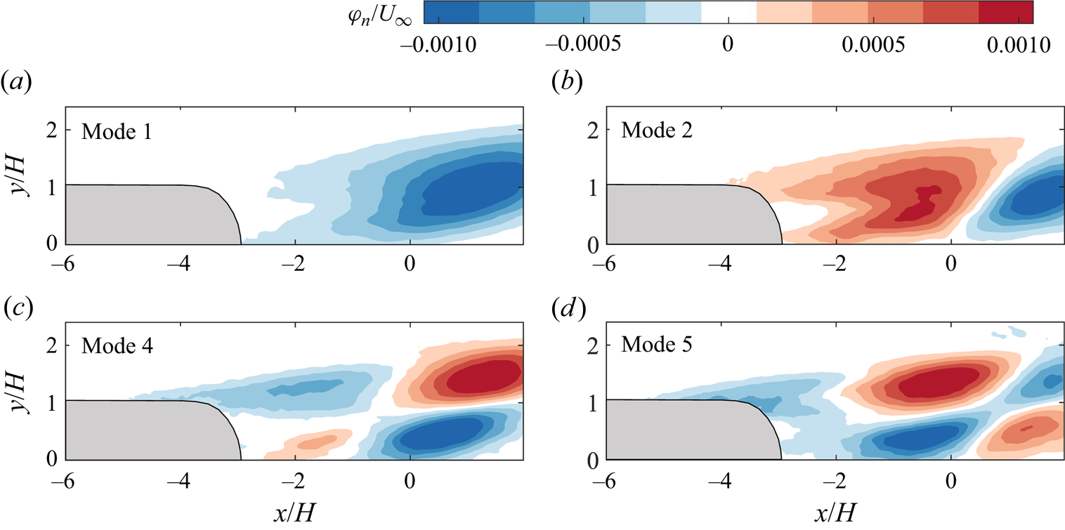
The modes 1, 2, 4 and 5 at the finlet plane of the S3 case are selected to represent the unsteady flow features, as shown by the streamwise velocity fluctuation component ( $\varphi _{n}/U_\infty$) in figure 16. The modes related to the wall-attached eddies in the untreated turbulent boundary layer are modified significantly by the finlets, exhibiting changes in pattern and shape (Feng & Ye Reference Feng and Ye2023). Mode 1 (figure 16a) is dominated by a large-scale low-speed fluctuation patch of more than
 $5H$ length, which is related to the large-scale velocity streaks. The inclination angle of the patch increases to
 $20^\circ$ compared with that of the untreated condition, featuring an arch shape with the apex pointing towards the downstream direction. The former patch detaches slightly from the wall due to the lift-up effect induced by the finlets, which is attributed to the induced upwash motion and the mutual interaction between the detached and near-wall shear layers. Mode 2 (figure 16b) features alternative high- and low-speed fluctuation patches with decreasing wavelength and similar patch shape, corresponding to the large-scale velocity streaks similar to mode 1.
Streamwise velocity fluctuation component ( $\varphi _{n}/U_\infty$) of POD modes at the finlet plane for the S3 case: (a) mode 1, (b) mode 2, (c) mode 4 and (d) mode 5.

For modes 4 and 5 (figure 16c,d), a different pattern emerges, being related to the flow features induced by the finlets. The streamwise velocity fluctuation patches of alternative signs appear at the detached and near-wall shear layers, corresponding to the generation of detached hairpin-like vortices and spanwise rollers, respectively. The length and height of each patch decrease remarkably. The velocity fluctuation patches hold opposite signs in the wall-normal direction, possibly inducing the wall-normal undulation of the structures (Humble Reference Humble2008) and intensifying the interaction between the two shear layers. The overall distribution indicates an upward movement, which is in agreement with the observation in the instantaneous flow field.
7. Relation between wall-pressure and velocity fluctuations
7.1. Frequency-dependent pressure–velocity coherence
Based on the Poisson equation, the turbulent structures and induced velocity gradient are responsible for the generation of wall-pressure fluctuations (Thomas & Bull Reference Thomas and Bull1983). The streamwise finlets lead to a redistribution of turbulent structures. In order to understand the effect of turbulent structures on the wall-pressure fluctuations, the frequency-dependent pressure–velocity coherence analysis is performed. The non-dimensionalised cross-spectrum between the velocity and the wall-pressure fluctuations is calculated at the streamwise location of the wall-pressure transducer ( $x/H = -1.54$), following Zang, Mayer & Azarpeyvand (Reference Zang, Mayer and Azarpeyvand2020) as
 \begin{equation} C_{p u_i}(f, y)=\frac{\left|\phi_{p u_i}(f, y)\right|^2}{\phi_{p p}(f) \phi_{u_i u_i}(f, y)}\left(\frac{u_{r m s}^{\prime}(y)}{U_{\infty}}\right)^2, \end{equation}
where  $\phi _{u_i u_i}$ is the PSD of the velocity fluctuation components (
 $u^\prime _i$),
 $\phi _{p u_i}$ represents the cross-spectral density between
 $p^\prime$ and
 $u^\prime _i$, and
 $u_{r m s}^{\prime }$ is the root-mean-square of the streamwise velocity fluctuations. The results are shown in figure 17 for the untreated and S3-F cases, considering both streamwise (
 $u^\prime$) and wall-normal (
 $v^\prime$) velocity fluctuations.
Pressure-velocity coherence ( $C_{p u_i}$) at
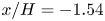 $x/H = -1.54$: (a,c) streamwise velocity fluctuations (
 $u'$); (b,d) wall-normal velocity fluctuations (
 $v'$); (a,b) untreated case; (c,d) S3-F case.

For the untreated case (figure 17a,b), the coherence extends from the wall to  $y/H < 1.1$ and
 $y/H < 1.3$ for
 $C_{pu}$ and
 $C_{pv}$, respectively. According to the coherence patterns of different scales, the spectra are divided into low-, mid- and high-frequency bands by inspecting the representing features, being segmented at
 $f = 320$ and 1560 Hz as shown by the white dashed lines. Following Gibeau & Ghaemi (Reference Gibeau and Ghaemi2021), it is assumed that the convection velocity (
 $U_c$) is the mean velocity at the half-height of the coherence region of
 $C_{pv}$ (
 $\kern 1.5pt y = 0.65H$), yielding
 $U_c \approx 0.7U_\infty$ at
 $x/H = -1.54$. Therefore, in the low-frequency band (
 $\,f < 320\,{\rm Hz}$), the corresponding length scale of the coherent structures (
 $\lambda$) falls above about
 $3\delta _{99}$ (
 $\delta _{99}$ is the boundary layer thickness at
 $x = -20$ mm, representing the average boundary layer thickness on the airfoil surface in the measurement region), indicating the dominance of large-scale velocity streaks. The coherence between
 $p$ and
 $u$ is more than an order magnitude higher than that between
 $p$ and
 $v$ close to the wall (
 $\kern 1.5pt y/H<0.2$), revealing the importance of the streamwise component of the turbulent structures on the pressure fluctuations in the low-frequency band (Naka et al. Reference Naka, Stanislas, Foucaut, Coudert, Laval and Obi2015; Gibeau & Ghaemi Reference Gibeau and Ghaemi2021). A higher level of coherence appears in the mid-frequency band (
 $\,f = [320, 1560]$ Hz,
 $\lambda /\delta _{99} = [0.6, 3]$). Different from the low-frequency band, the contribution of the wall-normal fluctuation component (
 $v^\prime$) surpasses that of the streamwise component (
 $u^\prime$), indicating the dominance of large-scale hairpin vortices in this range (Adrian Reference Adrian2007). The wall-normal location of high coherence decreases with increasing frequency. This phenomenon agrees with the attached-eddy hypothesis (Hutchins & Marusic Reference Hutchins and Marusic2007; Chandran, Monty & Marusic Reference Chandran, Monty and Marusic2020; de Silva et al. Reference de Silva, Chandran, Baidya, Hutchins and Marusic2020), as the smaller wall-attached eddies are located closer to the wall. In the high-frequency band (
 $\,f > 1560$ Hz,
 $\lambda /\delta _{99} < 0.6$), the overall coherence level decreases, with the peak location moving closer to the wall due to the dominant contribution from small-scale structures. These results are similar to the case of Gibeau & Ghaemi (Reference Gibeau and Ghaemi2021), who measured the pressure and velocity coherence of a turbulent boundary layer over a flat plate. One can see that the separator of the low- and mid-frequency bands is similar to that segregating the increase and decrease of the wall-pressure fluctuations (figure 9), which further implies the close relationship between the modification of turbulent structures of different scales and the suppression of wall-pressure fluctuations.
The distribution of pressure–velocity coherence changes remarkably with the presence of the finlets. At the finlet plane (figure 17c,d),  $C_{pv}$ intensifies significantly in the low-frequency band, becoming much higher than
 $C_{pu}$, which is due to the induced upwash and downwash motions by the finlet-induced structures. On the other hand, both
 $C_{pu}$ and
 $C_{pv}$ are weakened significantly in the mid-frequency band and become almost negligible in the high-frequency band, indicating the disruption of large-scale hairpin vortices and small-scale motions of the untreated case close to the wall (Ghaemi & Scarano Reference Ghaemi and Scarano2013; Gibeau & Ghaemi Reference Gibeau and Ghaemi2021). The result agrees with the reduction of pressure fluctuations in the former bands (figure 9). The coherence range of two velocity components extends up to
 $y/H = 1.5$ due to the finlet-induced structures and the lift-up process. For the
 $p$–
 $u$ coherence (figure 17c), the broadband spectra of high coherence are demarcated into two areas (yellow dashed line at
 $y/H = 0.75$) due to the presence of the detached and near-wall shear layers. The coherence related to the detached shear layer is weaker than that closer to the wall. However, for the
 $p$–
 $v$ coherence (figure 17d), the former spatial separation of high coherence only appears in the high-frequency and part of the mid-frequency bands. This is related to the mutual interaction of the two shear layers, which also leads to an overall uplift of the high coherence region of both
 $C_{pu}$ and
 $C_{pv}$ compared with the untreated case.
7.2. Bandpass filtered Reynolds shear stress
The coherence between the wall-pressure and velocity fluctuations indicates three distinct frequency bands, with specific association with the scales of turbulent structures. Hereby, the relationship between the coherent structures of different frequency bands with the Reynolds shear stress ( $-\overline {u^{\prime } v^{\prime }} / U_{\infty }^2$) is quantified by the bandpass filtered streamwise and wall-normal velocity fluctuations. The cross-plane contours of the Reynolds shear stress at different frequency bands for the untreated and S3-F cases are shown in figure 18. For the untreated case (figure 18a,c,e), the Reynolds shear stress indicates a broadband nature, with local maxima appearing in all three frequency bands. The maximum shear stress focuses on the mid-frequency band, with the peak centred at around
 $y/H = 0.3$. The former location corresponds to the logarithmic region of the turbulent boundary layer, within which large-scale vortices and hairpin packets are populated (Adrian Reference Adrian2007).
Contours of bandpass filtered Reynolds shear stress at  $x\unicode{x2013}y$ cross-plane: (a,c,e) untreated case; (b,d,f) S3-F case; (a,b), (c,d) and (e,f) represent low-, mid- and high-frequency bands, respectively. The yellow and green dashed lines indicate the detached and near-wall shear layers, respectively.

For the S3 case at the finlet plane (figure 18b,d,f), the distribution of shear stress is modified significantly in all three frequency bands. In the low-frequency band (figure 18b), the near-wall shear layer produces higher shear stress compared with the untreated case (green dashed line). While the detached shear layer is much weaker (yellow dashed line). In the mid-frequency band (figure 18d), the reminiscence of the near-wall shear layer with a similar magnitude can still be observed, exhibiting a larger inclination angle due to the stronger lift-up effect for higher frequencies. The detached shear layer atop the finlets starts to be strengthened, related to the generation of hairpin-like vortices. In addition, the high-shear layer in the logarithmic regime of the untreated turbulent boundary layer cannot be detected, in agreement with the distortion of the coherent structures in this regime (figure 17). In the high-frequency band (figure 18f), the detached shear layer undergoes decaying processes when evolving downstream. On the other hand, the near-wall shear layer disappears in this range. As described by Na & Moin (Reference Na and Moin1998) and Abe (Reference Abe2017), a strong relationship exists between the local Reynolds shear stress and the wall-pressure fluctuations. The reduction of near-wall shear stress in the mid- and high-frequency bands with the finlet treatment is in accordance with the suppression of wall-pressure fluctuations (Kim Reference Kim1983; Kobashi & Ichijo Reference Kobashi and Ichijo1986).
7.3. Patterns of pressure–velocity correlation
In order to directly identify the patterns of coherent structures correlated with the production of the wall-pressure fluctuations, the pressure–velocity correlation is investigated, being defined as
 \begin{equation} R_{p u_i}(x, y)=\frac{1}{\rho U_{\infty}^3}\left\langle p^{\prime}(t) u_i^{\prime}(x, y, t)\right\rangle, \end{equation}
where  $p^\prime$ is the wall-pressure fluctuations sampled at
 $x/H = -1.54$, and the use of
 $\langle \cdots \rangle$ denotes an ensemble average in time. Based on the spectra of pressure–velocity coherence, the wall-pressure fluctuation signal is bandpass filtered into low-, mid- and high-frequency bands (being referred to as
 $p_L^\prime$,
 $p_M^\prime$ and
 $p_H^\prime$, respectively). The corresponding turbulent motions contributing to the generation of wall-pressure fluctuations within each band are revealed by the spatial distribution of
 $R_{p u_i}$,
 $R_{p u_i}^L$,
 $R_{p u_i}^M$ and
 $R_{p u_i}^H$ in the
 $x\unicode{x2013}y$ plane, respectively, as shown in figure 19 for the untreated and S3-F cases.
Spatial distribution of the pressure-streamwise velocity ( $p$–
 $u$) correlation from different frequency bands: (a,b) full, (c,d) low frequency, (c,d) mid frequency and (c,d) high frequency; (a,c,e,g) untreated case; (b,d,f,h) S3-F case. The black dashed lines represent the location of the pressure transducer.

For the untreated case, the  $p$–
 $u$ correlation for the full-frequency band (
 $R_{p u}$, figure 19a) features a region of positive correlation directly above the pressure transducer and extending towards the upstream direction. The former region has a height of
 $1H$ and extends upstream to
 $x/H = -3$. A negative correlation region right downstream of the positive one with a height of
 $1.2H$ extends downstream to
 $x/H = 1$, being almost symmetric to each other with respect to the location of the pressure transducer. This is similar to the results over a flat plate by Naka et al. (Reference Naka, Stanislas, Foucaut, Coudert, Laval and Obi2015) and Gibeau & Ghaemi (Reference Gibeau and Ghaemi2021). However, a larger and stronger negative correlation region is observed here, which is possibly induced by the adverse pressure gradient over an airfoil. The pattern with alternative positive and negative correlation peaks is related to two motions: a strong sweep motion appears upstream of the transducer, followed by an ejection motion downstream (Thomas & Bull Reference Thomas and Bull1983) and the hairpin-induced upstream ejection and downstream sweep motions (Ghaemi & Scarano Reference Ghaemi and Scarano2013). When considering the pressure fluctuations of different scales after the bandpass filter (figure 19c,e,g), the overall distribution is similar to that of the full-frequency band. However, the scale and shape of the correlation pattern change significantly. In the low-frequency band (
 $R_{p u}^L$, figure 19c), the positive and negative correlation regions feature with a more elongated shape of approximately
 $3H$, being further inclined towards the wall. The former regions are related to the large-scale velocity streaks, as proposed in the attached eddy model (Gibeau & Ghaemi Reference Gibeau and Ghaemi2021). In the mid-frequency band (
 $R_{p u}^M$, figure 19e), the intensity of
 $p$–
 $u$ correlation increases significantly close to the wall, with an almost identical scale compared with that of the full-frequency band. Weaker correlation peaks appear at the upstream and downstream sides of those close to the pressure transducer. The former correlation peaks are associated with hairpin structures, which induce strong sweep and ejection events and have a significant impact on wall-pressure fluctuations (Thomas & Bull Reference Thomas and Bull1983; Kobashi & Ichijo Reference Kobashi and Ichijo1986; Gibeau & Ghaemi Reference Gibeau and Ghaemi2021). In the high-frequency band (
 $R_{p u}^H$, figure 19g), the correlation weakens. Only low-intensity correlation peaks of alternating signs are observed near the pressure transducer, confining in the region below
 $y/H = 0.4$. The characteristics indicate that the coherent structures and pressure fluctuations are mainly correlated in the low- and mid-frequency bands.
A remarkable modification of  $p$–
 $u$ correlation is produced by the finlet treatment, as shown in figure 19(b,d,f,h). Comparing different frequency bands, it is evident that the flow structures in the low-frequency band (
 $R_{p u}^L$, figure 19d) play a crucial role in wall-pressure fluctuations due to the similar correlation pattern with respect to the full-frequency band. The correlation pattern is recognised as two major areas. The dominant area is located close to the wall, which is associated with the near-wall shear layer. It is composed of a relatively small positive correlation region of
 $0.5H$ height upstream of and towards the pressure transducer, followed by a larger negative correlation region of
 $1H$ height downstream. Both regions have a higher correlation compared with the untreated case. The second strongly correlated region is located over the finlets away from the wall, which is related to the detached shear layer. The interconnection between the top and bottom correlation peaks is observed, indicating a coupling effect. In the mid-frequency band (
 $R_{p u}^M$, figure 19f), a significant overall attenuation of
 $p$–
 $u$ correlation is observed compared with the untreated case. The correlation peaks of alternating signs at the detached shear layer with a smaller magnitude and wavelength (about
 $1H$ length) become predominant. The influence of the flow separation in the near-wall area becomes trivial. In the high-frequency band (
 $R_{p u}^H$, figure 19h), the correlation region weakens significantly and becomes almost invisible. These results align with the observed increase at low frequencies and decrease at mid and high frequencies of the wall-pressure fluctuations PSD results in figure 9.
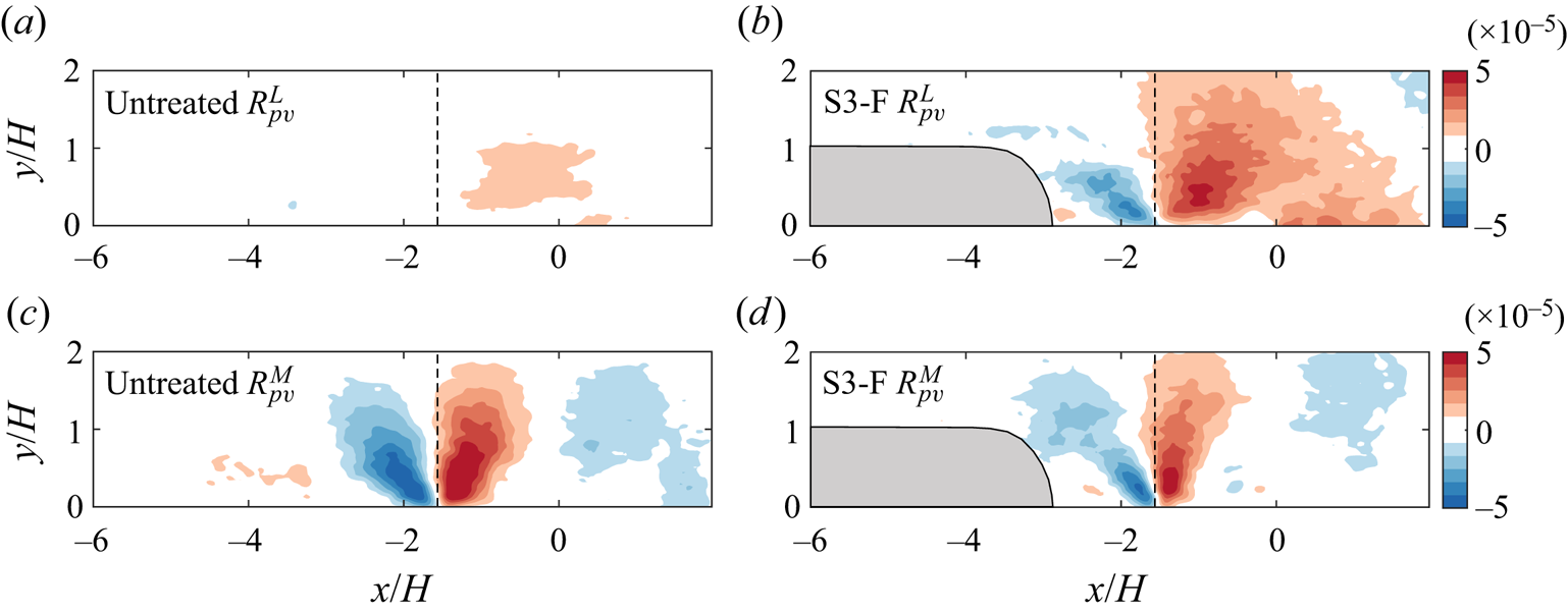
The correlation between the pressure fluctuations and wall-normal velocity fluctuations ( $p$–
 $v$ correlations) is performed in the low- and mid-frequency bands, as shown in figure 20. In the low-frequency band, for the untreated case (
 $R_{p v}^L$, figure 20a), the
 $p$–
 $v$ correlation is much lower than the
 $p$–
 $u$ correlation, which is similar to the results of Gibeau & Ghaemi (Reference Gibeau and Ghaemi2021). However, the finlet case (
 $R_{p v}^L$, figure 20b) exhibits much larger and stronger correlation regions, with the negative and positive correlation regions appearing upstream and downstream of the pressure transducer, respectively. The high-correlation peaks involve the region of the two shear layers, indicating the coupling effect. The mutual interaction of the two shear layers induces stronger downwash and upwash motions, contributing to the increase of pressure fluctuations at low frequencies. Then, in the mid-frequency band (
 $R_{p v}^M$, figure 20c,d), both the two cases are composed of elongated negative and positive correlation regions, being symmetric to the location of the pressure transducer. The coupling of the two shear layers is still observed. However, the magnitude and region of correlation for the finlet case indicate a notable reduction, which is in accordance with the pressure fluctuation PSD results in the mid-frequency band.
Spatial distribution of the pressure-wall-normal velocity ( $p$–
 $v$) correlation: (a,b) low-frequency band; (c,d) mid-frequency band; (a,c) untreated case; (b,d) S3-F case. The black dashed lines represent the location of the pressure transducer.

The scenario confirms that the presence of the finlets significantly disrupts and redistributes the coherent structures in the turbulent boundary layer. The newly generated structures produced at near-wall and detached shear layers dominate the pressure fluctuations in the low- and mid-frequency bands, respectively. The suppression of the large-scale hairpin vortices of the untreated case and the disappearance of the small-scale motions contribute to the noise reduction in the mid- and high-frequency bands.
7.4. Conditional averaging based on HAPPs
To directly characterise the dominant turbulent structures related to the wall-pressure fluctuations, the conditional averaging based on the occurrence of both positive and negative HAPPs is performed for the instantaneous velocity fields (Antonia Reference Antonia1981; Ghaemi & Scarano Reference Ghaemi and Scarano2013). The HAPPs are conformed when the positive and negative pressure fluctuation peaks exceed a certain threshold. The velocity fluctuation component  $u'_i$ in the measurement domain is sampled at every occurrence of HAPPs. The details of the conditional averaging are shown as
 \begin{equation} \left. \begin{gathered} u_{i, H A P P s^{+}}^{\prime}(x, y)=\frac{1}{N} \sum_{j=1}^N u_i^{\prime}(x, y, t) ,\quad \text{when}\ p_{peak }^{\prime}(t)>\alpha p_{r m s}^{\prime},\\ u_{i, H A P P s^{-}}^{\prime}(x, y)=\frac{1}{N} \sum_{j=1}^N u_i^{\prime}(x, y, t), \quad \text{when}\ p_{peak }^{\prime}(t)<{-}\alpha p_{r m s}^{\prime}, \end{gathered} \right\} \end{equation}
where  $u_{i, HAPPs^{+}}^{\prime }$ and
 $u_{i, HAPPs^{-}}^{\prime }$ denote the conditional-averaged velocity fluctuation component based on positive and negative HAPPs events, respectively. Here
 $p_{peak }^{\prime }$ and
 $p_{r m s}^{\prime }$ is the peak and root-mean-square of the pressure fluctuations, respectively, being sampled at
 $x/H = -1.54$. We use
 $\alpha$ to denote a threshold limit, which is chosen to be 2 in the present investigation (Ghaemi & Scarano Reference Ghaemi and Scarano2013), and
 $N$ is the total number of positive or negative HAPP events within 12 000 samples, which is shown in figure 21 for different configurations. Compared with the untreated case, the number of HAPPs with finlet treatment decreases significantly for both the finlet and mid planes, which is attributed to the modification of the finlet-induced structures and the near-wall velocity deficit. In addition, a larger number of positive HAPPs is obtained compared with the negative HAPPs for all the cases, indicating a greater contribution of the former events to the overall-pressure fluctuation energy.
Number of the positive and negative HAPPs of different configurations.

Regarding the conditional-averaged streamwise velocity field, for the untreated case in figure 22(a), a high-speed structure directly above the pressure transducer is observed when positive HAPPs occur, which extends upstream to  $x/H = -3$ with a height of
 $0.8H$. A rather weaker low-speed structure follows the high-speed one and locates downstream the pressure transducer, which extends to the airfoil trailing edge wake of
 $x/H = 0.5$ with a height of
 $0.45H$. The high-speed structure plays a dominant role in inducing strong sweep events upstream of the pressure transducer, followed by weak ejection events downstream. For the coherent structure related to negative HAPPs as shown in figure 22(b), only large-scale high-speed structure is observed, which moves downstream of the pressure transducer and produces a strong sweep event (Ghaemi & Scarano Reference Ghaemi and Scarano2013). The results reveal that the large-scale high-speed structures have a predominant influence on the generation of HAPPs, similar to the observation of Naka et al. (Reference Naka, Stanislas, Foucaut, Coudert, Laval and Obi2015).
Cross-plane contours of conditional averaged streamwise velocity fluctuations ( $u^\prime /U_\infty$) based on the occurrence of HAPPs, respectively, superimposed with vector field: (a,c) positive HAPPs; (b,d) negative HAPPs; (a,b) untreated case; (c,d) S3-F case. The purple dashed lines represent the location of the pressure transducer.

At the finlet plane (figure 22c,d), the turbulent coherent structures contributing to the generation of positive and negative HAPPs are associated with the hairpin-like structures and spanwise vortices located at the detached and near-wall shear layers. The coherence of turbulent structures reduces globally. An overall lift-up effect of the coherent structures is observed, reducing their contribution to the near-wall-pressure fluctuations. For the positive HAPPs (figure 22c), the high-speed streak directly above the pressure transducer remains to be predominant. The size of the former structure reduces to  $0.5H$ height and
 $1H$ length compared with the untreated case, being followed by a weaker low-speed streak of much larger size of
 $1H$ height and
 $2H$ length. Since the positive HAPPs are caused by the sweep events of the hairpin vortices in the log layer for the untreated case (Ghaemi & Scarano Reference Ghaemi and Scarano2013), the reduction in the structure size and intensity of the sweep motion confirms the disruption of the former vortices. Moreover, the velocity streaks related to the finlet-induced hairpin-like vortices emerge at the detached shear layer away from the wall, indicating a correlation with pressure fluctuation irrespective of the spatial separation. The connected vectors between the two shear layers indicate the coupling effect. Due to the mutual interaction of the two shear layers, sweep and ejection motions of reduced magnitude compared with the untreated case are induced on the upstream and downstream sides of the pressure transducer, respectively, as shown by the vector field. The coherent structures related to negative HAPPs (figure 22d) exhibit phase inversion spatially compared with the positive HAPPs, with the positive velocity streaks located downstream of the pressure transducer. The sweep motion extends to a larger area due to the interaction between the detached and near-wall structures, possibly contributing to the increase of low-frequency increase of pressure fluctuations.
8. Conclusions
In the present study, the finlet treatments of three spanwise spacings ( $S = 12$ mm, 6 mm and 3 mm) are applied close to the trailing edge of a NACA0018 airfoil to obtain wall-pressure fluctuation and far-field noise suppression. The main focus was to understand the effect of finlets on the evolution of unstable turbulent structures and their contribution to surface pressure fluctuations. The instantaneous velocity field and wall-pressure fluctuations have been measured simultaneously by time-resolved PIV and wall-pressure transducers to build a direct quantitative correlation. The inspection of the far-field noise indicates a noise reduction in the frequency range of 400–2000 Hz with the implementation of finlets. The maximum noise reduction of 2.7 dB has been obtained with the finlets with the smallest spanwise spacing (
 $S = 3$ mm). Similarly, the wall-pressure fluctuations at different locations have been suppressed in the former frequency range, indicating a close relation with the noise-reduction effect.
The time-averaged flow field indicates the formation of the detached and near-wall shear layers around and downstream of the finlets, due to the upwash motion and backward flow separation, respectively. The momentum redistribution induced by the finlets leads to a strong near-wall velocity deficit along the entire span of the airfoil. The lower velocity magnitude and reduced wall shear stress are in favour of the reduction of pressure fluctuations and noise scattering at the trailing edge.
In the instantaneous flow field, the turbulent coherent structures of the untreated condition are replaced by the hairpin-like vortices and spanwise rollers forming at the detached and near-wall shear layer, respectively. As indicated by the POD analysis, the disturbance energy related to the newly generated structures increases steeply. The mutual interaction between the turbulent structures at the two shear layers induces an overall lift-up process, which brings the most energetic turbulent structures away from the wall and leaves the eddies with lower energy in the near-wall region.
The relationship between wall-pressure and velocity fluctuations reveals that the disruption of hairpin-like and small-scale turbulent structures close to the airfoil surface and the lift-up process cause the reduction of  $p$–
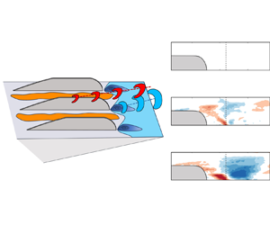
 $u$ coherence and correlation in the mid- and high-frequency bands. The former phenomenon contributes to the reduction of the near-wall shear stress and pressure fluctuations. Based on the conditional averaged velocity field, the large-scale structures of the untreated case leading to the occurrence of HAPPs are replaced by smaller-scale structures close to the wall with finlet treatment. As a result, the modification of turbulent structures and momentum redistribution is the major contributor to the mitigation of wall-pressure fluctuations and far-field noise. The conceptual sketch of the dominant flow features and the related wall-pressure signal are provided in figure 23.
Conceptual sketch of the finlet-induced structures and the variations of wall-pressure fluctuations.

One aspect to mention is the formation of flow separation and large-scale structures, which causes an unwanted increase in pressure fluctuations in the low-frequency band. In addition, finlet treatment will affect aerodynamic performance. Our current experiments have found that the S6 and S3 finlet treatments used in this application increase drag by approximately 21 % and 30 %, respectively. Further geometrical study of the finlets is necessary to provide an optimised design and to obtain broadband pressure and noise reduction with a small aerodynamic penalty.
Supplementary movies
Supplementary movies are available at https://doi.org/10.1017/jfm.2024.1192.
Funding
This work was supported by National Natural Science Foundation of China (grant number 12372280) and National Key R&D Program of China (grant number 2020YFA0405700).
Declaration of interests
The authors report no conflict of interest.