1. Introduction
The phenomenon in which a solid phase moves in a liquid phase while undergoing melting and solidification, which is observed in the transport of phase change materials such as ice slurry flows (Wang et al. Reference Wang, Battaglia, Wang, Zhang and Ma2019), is interesting in fluid mechanics and important in various engineering fields. The governing equations of this system are composed of the equation of motion of the solid phase, the equation of motion of the liquid phase, the advection–diffusion equation of temperature and the Stefan condition (Juric & Tryggvason Reference Juric and Tryggvason1996; Udaykumar, Mittal & Shyy Reference Udaykumar, Mittal and Shyy1999) representing the movement of the solid-phase surface due to melting and solidification. The liquid and solid phases exchange the mass, momentum and energy across their interface. Thus, this phenomenon is a complex system involving the motions of the liquid and solid phases, heat transfer in each phase and phase change.
When the solid phase is treated as a rigid body, its equations of motion should be expressed in a form that incorporates the effects of melting and solidification into the equations for rigid-body dynamics. In previous studies, regardless of whether a solid particle melts and solidifies uniformly while maintaining a spherical shape (Dierich, Nikrityuk & Ananiev Reference Dierich, Nikrityuk and Ananiev2011; Shabgard et al. Reference Shabgard, Hu, Boettcher, McCarthy and Sun2016) or non-uniformly (Gan, Feng & Hu Reference Gan, Feng and Hu2003; Sakane et al. Reference Sakane, Takaki, Ohno and Shibuta2019; Guo et al. Reference Guo, Zhang, Meng, Zhang and Poncet2020), the motion of the solid particle has been described simply by the following well-known Newton–Euler equations of motion for a rigid body:
 \begin{align}&M\frac {\mathrm{d} \boldsymbol{u}_{\textit{c}}}{\mathrm{d}t} = \boldsymbol{F},\end{align}
 \begin{align} &\mathcal{I}\frac {\mathrm{d}\boldsymbol{\omega }_{\textit{c}}}{\mathrm{d}t} + \boldsymbol{\omega }_{\textit{c}} \times (\mathcal{I}\boldsymbol{\omega }_{\textit{c}}) = \boldsymbol{T},\end{align}
where
 $M$
is the mass,
 $\boldsymbol{u}_{\textit{c}}$
is the velocity of the centre of mass (COM),
 $\boldsymbol{F}$
is the external force including the gravitational force and the fluid force exerted by the ambient liquid phase,
 $\mathcal{I}$
is the inertia tensor,
 $\boldsymbol{\omega }_{\textit{c}}$
is the angular velocity, and
 $\boldsymbol{T}$
is the external torque including the gravitational torque and the fluid torque. It is noted that
 $\mathcal{I}$
,
 $\boldsymbol{\omega }_{\textit{c}}$
and
 $\boldsymbol{T}$
are defined about the COM. Notably, the mass
 $M$
and inertia tensor
 $\mathcal{I}$
vary in time due to melting and solidification. At first glance, this may appear reasonable; however, considering that the mass
 $M$
changes, the following simple question arises.
-
Q1. Newton’s second law of motion says ‘The change of momentum of an object is proportional to the force impressed.’ Thus, should the left-hand side of (1.1) be
 $\mathrm{d}(M\boldsymbol{u}_{\textit{c}})/\mathrm{d}t?$

If the answer of this question is yes, the left-hand side of (1.1) should be corrected by adding a term
 $\dot {M}\boldsymbol{u}_{\textit{c}}$
(where the dot denotes the time derivative), making the motion of the solid particle different. Actually, the answer has been given as ‘no’ by Crowe et al. (Reference Crowe, Schwarzkopf, Sommerfeld and Tsuji2011). They derived the equations of motion for a single particle undergoing burning, evaporation or condensation by using the Reynolds transport theorem, and they showed that the term
 $\dot {M}\boldsymbol{u}_{\textit{c}}$
cancels out a part of the momentum flux through the particle surface. The same conclusion should be obtained in the case of melting and solidification, since these processes are included in the premises of their derivation. However, to the best of the authors’ knowledge, none of the studies that analyses melting and solidification has taken this fact into account.
In addition, when a particle melts and solidifies non-uniformly, its COM should shift due to deformation; however, (1.1) and (1.2) do not explicitly include the terms corresponding to this effect. Therefore, the following question also arises.
-
Q2. Should (1.1) and (1.2) include the terms representing the effect of the COM shift due to deformation?
This question has not been discussed in any previous studies, even by Crowe et al. (Reference Crowe, Schwarzkopf, Sommerfeld and Tsuji2011).
In the present study, to address questions Q1 and Q2, we derive the equations of motion for a solid phase undergoing melting and solidification, following the derivation of the governing equations of fluid mechanics. As a basic assumption, the surface of the solid-phase region deforms at a velocity determined by the Stefan condition (hereafter, we call it the Stefan velocity), due to melting and solidification. Thus, it can be interpreted that mass, momentum and angular momentum fluxes pass through the solid-phase surface at the Stefan velocity. In addition, the momentum fluxes by the jet due to density change should be considered as well. By equating the sum of these momentum fluxes and the external force to the time derivative of the linear momentum of the solid phase, we derive the translational equation of motion. Similarly, by considering the angular momentum balance, we derive the rotational equation of motion. We compare the derived equations with (1.1) and (1.2) and then discuss the effects raised in questions Q1 and Q2.
Before proceeding, we briefly explain why an analytical mechanics approach using a Lagrangian is not adopted in the present work. The present system consists of solid and liquid phases, and one phase changes into the other through melting and solidification. In principle, the Lagrangian of the system should therefore include contributions from both phases. However, the difficulty arises because the mass of each phase is not conserved separately: the solid phase continuously exchanges mass with the liquid phase due to phase change. As a result, the degrees of freedom associated with the solid and liquid phases are not fixed, but continuously exchanged, which makes it non-trivial to define a single Lagrangian for the combined system. If we define the Lagrangian only for the solid phase, we must incorporate the Lagrangian flux from and to the liquid phase in the action (the time integral of the Lagrangian). Such a flux can be interpreted as a non-holonomic constraint, and would appear as momentum and angular momentum fluxes in the Lagrange equations derived from the action principle. Although introducing such a Lagrangian flux is essentially equivalent to considering the momentum and angular momentum fluxes, the latter formulation seems physically clearer. Therefore, in the present work, we adopt the conservation laws of momentum and angular momentum rather than a Lagrangian formulation.
The remainder of this paper is structured as follows. Section 2 describes the kinematics of the solid phase moving in liquid phase while melting and solidification. Section 3 derives the equations of motion of the solid phase. Section 4 summarises the derived equations and discusses questions Q1 and Q2. Finally, § 5 concludes the study.
2. Kinematics of solid phase
We consider the system where a finite solid-phase region
 $\varOmega$
moves in an infinite liquid-phase region. The solid-phase region
 $\varOmega$
moves as a rigid body, and its surface
 $\partial \varOmega$
deforms due to melting and solidification.
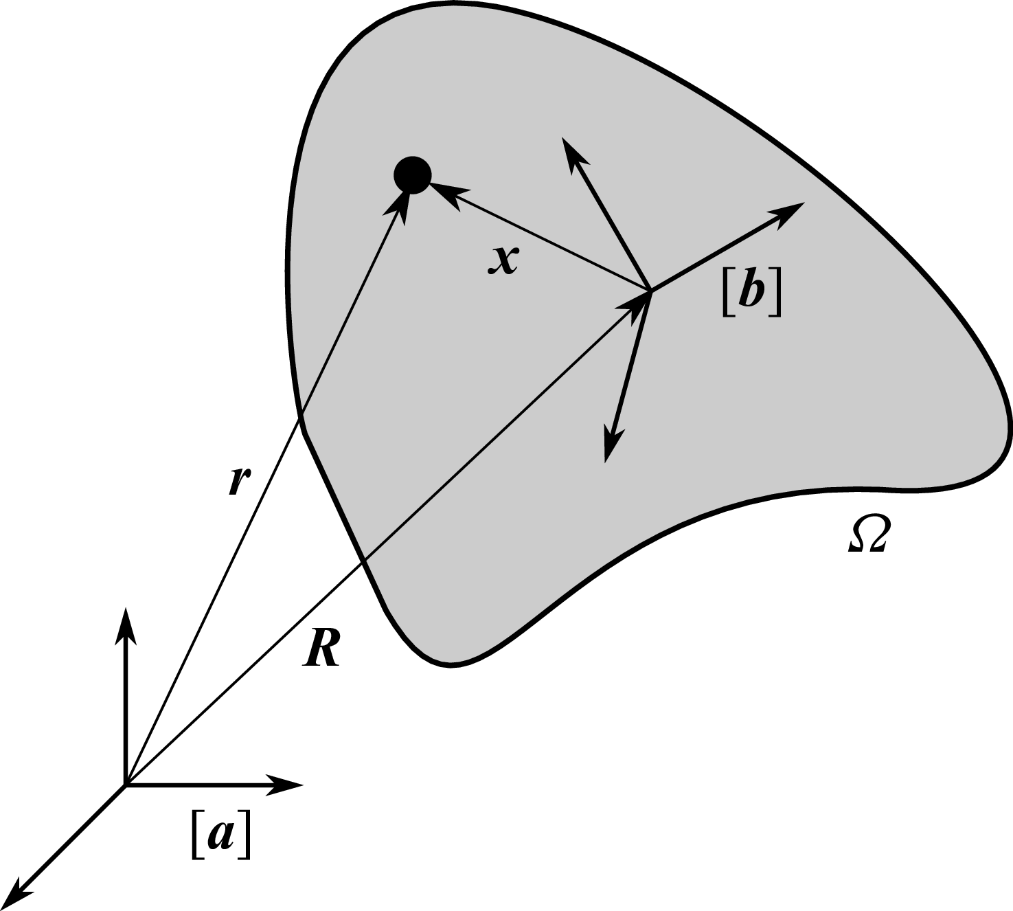
Coordinate system
 $[\boldsymbol{a}]$
fixed to the space and coordinate system
 $[\boldsymbol{b}]$
fixed to the solid-phase region
 $\varOmega$
. The position of the origin of
 $[\boldsymbol{b}]$
is denoted by the position vector
 $\boldsymbol{R}$
from the origin of
 $[\boldsymbol{a}]$
, and the position of an arbitrary point in
 $\varOmega$
is represented by the position vector
 $\boldsymbol{r}$
from the origin of
 $[\boldsymbol{a}]$
and by the relative position vector
 $\boldsymbol{x}$
from the origin of
 $[\boldsymbol{b}]$
.

2.1. Coordinate systems and velocity in the solid-phase region
At first, to describe the kinematics of the solid-phase region, we define the coordinate systems as shown in figure 1. We consider a right-handed orthonormal basis consisting of three basis vectors fixed to the space,
 $\boldsymbol{a}_1$
,
 $\boldsymbol{a}_2$
and
 $\boldsymbol{a}_3$
. By arranging these vectors as a row array, we define the basis-vector array as follows:
 \begin{align} [\boldsymbol{a}] = [\boldsymbol{a}_1,\boldsymbol{a}_2,\boldsymbol{a}_3], \end{align}
and refer to this as the space-fixed coordinate system (hereafter, the
 $[\boldsymbol{a}]$
-frame for simplicity).
Next, we introduce another right-handed orthonormal basis,
 $\boldsymbol{b}_1$
,
 $\boldsymbol{b}_2$
and
 $\boldsymbol{b}_3$
, whose origin is fixed at a point within the solid phase, and which translates and rotates together with the solid phase. In the same way as
 $[\boldsymbol{a}]$
, we define the basis-vector array as follows:
 \begin{align} [\boldsymbol{b}] = [\boldsymbol{b}_1,\boldsymbol{b}_2,\boldsymbol{b}_3], \end{align}
and refer to this as the body-fixed coordinate system (hereafter, the
 $[\boldsymbol{b}]$
-frame).
An arbitrary vector
 $\boldsymbol{V}$
is expressed by a linear combination of basis vectors as follows:
 \begin{align} \boldsymbol{V} &= [\boldsymbol{a}] \boldsymbol{V}^a = [\boldsymbol{a}_1, \boldsymbol{a}_2, \boldsymbol{a}_3] \left [\begin{array}{c} V^a_1 \\[4pt] V^a_2 \\[4pt] V^a_3 \end{array} \right ] = V^a_1 \boldsymbol{a}_1 + V^a_2 \boldsymbol{a}_2 + V^a_3 \boldsymbol{a}_3,\end{align}
 \begin{align}\boldsymbol{V} &= [\boldsymbol{b}] \boldsymbol{V}^b = [\boldsymbol{b}_1, \boldsymbol{b}_2, \boldsymbol{b}_3] \left [\begin{array}{c} V^b_1 \\[4pt] V^b_2 \\[4pt] V^b_3 \end{array} \right ] = V^b_1 \boldsymbol{b}_1 + V^b_2 \boldsymbol{b}_2 + V^b_3 \boldsymbol{b}_3,\end{align}
where
 $\boldsymbol{V}^a$
and
 $\boldsymbol{V}^b \in \mathbb{R}^3$
are the column vectors representing the components of
 $\boldsymbol{V}$
in the
 $[\boldsymbol{a}]$
- and
 $[\boldsymbol{b}]$
-frames, respectively. The superscripts
 $a$
and
 $b$
denote quantities expressed in the
 $[\boldsymbol{a}]$
- and
 $[\boldsymbol{b}]$
-frames, respectively. Throughout this paper, we use this notation to distinguish components expressed in the two coordinate systems.
The two coordinate systems are related through the rotation matrix
 $\mathcal{S}$
as follows:
 \begin{align} [\boldsymbol{b}] = [\boldsymbol{a}]\mathcal{S}, \end{align}
where
 $\mathcal{S}$
represents the orientation of the solid phase. From another viewpoint, the rotational matrix
 $\mathcal{S}$
is regarded as a function
 $\mathcal{S}: \mathbb{R}^3 \to \mathbb{R}^3$
, which maps components of a vector in the
 $[\boldsymbol{b}]$
-frame to components of a vector in the
 $[\boldsymbol{a}]$
-frame. Although
 $\mathcal{S}$
is commonly expressed in terms of Euler angles or quaternions, we do not specify a particular representation here, as the following discussion does not depend on it.
The position vector
 $\boldsymbol{r}$
of an arbitrary point within the solid-phase region
 $\varOmega$
can be expressed in terms of the position vector
 $\boldsymbol{R}$
of the origin of the
 $[\boldsymbol{b}]$
-frame and the relative position vector
 $\boldsymbol{x}$
measured from that origin as follows:
 \begin{align} \boldsymbol{r} &= \boldsymbol{R} + \boldsymbol{x}, \\[-12pt] \nonumber \end{align}
 \begin{align} &= [\boldsymbol{a}] \boldsymbol{R}^a + [\boldsymbol{b}] \boldsymbol{x}^b,\\[10pt] \nonumber \end{align}
where
 $\boldsymbol{R}^a \in \mathbb{R}^3$
is the column vector representing the coordinates of
 $\boldsymbol{R}$
in the
 $[\boldsymbol{a}]$
-frame and
 $\boldsymbol{x}^b \in \mathbb{R}^3$
represents the coordinates of
 $\boldsymbol{x}$
in the
 $[\boldsymbol{b}]$
-frame. Since the solid-phase region
 $\varOmega$
moves as a rigid body,
 $\boldsymbol{x}^b$
does not change with time.
The time derivative of the position vector
 $\boldsymbol{r}$
gives the velocity vector
 $\boldsymbol{u}_{\textit{b}}$
of an arbitrary point in
 $\varOmega$
. By using the dot notation (
 $\dot {\phantom {z}}$
) for the time derivative, we obtain
 \begin{align} \boldsymbol{u}_{\textit{b}} & = \dot {\boldsymbol{r}} = \dot {\boldsymbol{R}} + \dot {\boldsymbol{x}}, \\[-12pt] \nonumber \end{align}
 \begin{align} &= [\boldsymbol{a}] \dot {\boldsymbol{R}}^a + [\dot {\boldsymbol{b}}] \boldsymbol{x}^b, \\[-12pt] \nonumber \end{align}
 \begin{align} &= [\boldsymbol{a}] \big(\dot {\boldsymbol{R}}^a + \dot {\mathcal{S}} \boldsymbol{x}^b \big), \\[10pt] \nonumber \end{align}
where we have used the following three facts:
 $[\boldsymbol{a}]$
is fixed to the space and hence time-independent;
 $[\boldsymbol{b}]$
rotates with the solid phase and is related to
 $[\boldsymbol{a}]$
through (2.5);
 $\boldsymbol{x}^b$
is time-independent. The time derivative of the rotation matrix,
 $\dot {\mathcal{S}}$
, is related to the angular velocity vector
 $\boldsymbol{\omega }^b$
observed in the
 $[\boldsymbol{b}]$
-frame; see Appendix A for details of this relationship and its properties.
2.2. Deformation of the solid-phase surface due to melting and solidification
Let the density of the liquid phase be denoted by
 $\rho _{\textit{f}}$
and that of the solid phase by
 $\rho _{\textit{b}}$
. Throughout this paper, subscripts ‘f’ and ‘b’ are used to distinguish quantities associated with the liquid and solid phases, respectively. Let
 $L$
denote the latent heat of the solid phase per unit mass. The outward unit normal vector at an infinitesimal surface element
 $\mathrm{d}S$
on the solid-phase surface
 $\partial {\varOmega }$
is denoted by
 $\boldsymbol{n}$
. If the local deformation velocity on
 $\mathrm{d}S$
due to melting and solidification (hereafter referred to as the Stefan velocity) is denoted by
 $\boldsymbol{U}_{\textit{s}}$
, then the volumetric change of the solid phase per unit time is given by
 $\boldsymbol{U}_{\textit{s}} \boldsymbol{\cdot} \boldsymbol{n}\,\mathrm{d}S$
, and the corresponding mass change is
 $\rho _{\textit{b}} (\boldsymbol{U}_{\textit{s}}\boldsymbol{\cdot} \boldsymbol{n})\,\mathrm{d}S$
. Accordingly, the amount of heat released or absorbed per unit time due to melting and solidification is given by
 $\rho _{\textit{b}} L (\boldsymbol{U}_{\textit{s}}\boldsymbol{\cdot} \boldsymbol{n})\,\mathrm{d}S$
. From the energy conservation law, this quantity is equal to the difference between the heat fluxes from the liquid and solid phases on
 $\mathrm{d}S$
. Thus,
 \begin{align} \rho _{\textit{b}} L (\boldsymbol{U}_{\textit{s}}\boldsymbol{\cdot} \boldsymbol{n}) \,\mathrm{d}S = {(\boldsymbol{q}_{\textit{f}} - \boldsymbol{q}_{\textit{b}})}\boldsymbol{\cdot} \boldsymbol{n} \,\mathrm{d}S, \end{align}
where
 $\boldsymbol{q}_{\textit{b}}$
and
 $\boldsymbol{q}_{\textit{f}}$
are the heat flux vectors in the solid and liquid phases, respectively. Supposing that the Stefan velocity
 $\boldsymbol{U}_{\textit{s}}$
is parallel to the normal vector
 $\boldsymbol{n}$
, the Stefan condition (Juric & Tryggvason Reference Juric and Tryggvason1996; Udaykumar et al. Reference Udaykumar, Mittal and Shyy1999) is obtained as follows:
 \begin{align} \boldsymbol{U}_{\textit{s}} = \frac {1}{\rho _{\textit{b}} L}\left [ {(\boldsymbol{q}_{\textit{f}} - \boldsymbol{q}_{\textit{b}})}\boldsymbol{\cdot} \boldsymbol{n}\right ] \boldsymbol{n}. \end{align}
Since the heat flux vectors
 $\boldsymbol{q}_{\textit{b}}$
and
 $\boldsymbol{q}_{\textit{f}}$
are determined by the temperature gradients in each phase, the temperature fields of both phases must be known. In this study, however, we do not consider the temperature fields; instead, the Stefan velocity
 $\boldsymbol{U}_{\textit{s}}$
is treated as a given quantity.
2.3. Boundary condition of the liquid phase on the solid-phase surface
Related to the Stefan velocity given in the previous subsection, we discuss the boundary condition of the liquid phase on the surface of the solid-phase region.
From §§ 2.1 and 2.2, the solid-phase surface
 $\partial {\varOmega }$
moves not only with the rigid-body velocity given by (2.10), but also with the Stefan velocity due to melting and solidification, given by (2.12). Thus, the velocity of the solid-phase surface is expressed as
 $\boldsymbol{u}_{\textit{b}}+\boldsymbol{U}_{\textit{s}}$
. From the mass conservation law, the mass fluxes from the solid and liquid phases relative to the solid-phase surface must be identical. Therefore, the velocities of the solid phase
 $\boldsymbol{u}_{\textit{b}}$
and the liquid phase
 $\boldsymbol{u}_{\textit{f}}$
satisfy the following relation:
 \begin{align} \rho _{\textit{b}} \left [ \boldsymbol{u}_{\textit{b}} - (\boldsymbol{u}_{\textit{b}} + \boldsymbol{U}_{\textit{s}})\right ] \boldsymbol{\cdot} \boldsymbol{n} = \rho _{\textit{f}} \left [ \boldsymbol{u}_{\textit{f}} - (\boldsymbol{u}_{\textit{b}} + \boldsymbol{U}_{\textit{s}})\right ] \boldsymbol{\cdot} \boldsymbol{n}\quad (\text{on}\,\partial {\varOmega }). \end{align}
This relation corresponds to the interfacial velocity jump condition at the interface in evaporation and condensation processes, where large volumetric changes occur (Gibou et al. Reference Gibou, Chen, Nguyen and Banerjee2007). Furthermore, under the no-slip condition at the solid-phase surface, the velocity components normal to
 $\boldsymbol{n}$
for
 $\boldsymbol{u}_{\textit{b}}$
and
 $\boldsymbol{u}_{\textit{f}}$
should be identical on the solid-phase surface. Therefore, the velocity of the liquid phase
 $\boldsymbol{u}_{\textit{f}}$
should satisfy the following boundary condition on the solid-phase surface:
 \begin{align} \boldsymbol{u}_{\textit{f}} = \boldsymbol{u}_{\textit{b}} + \left ( 1-\frac {\rho _{\textit{b}}}{\rho _{\textit{f}}} \right )\boldsymbol{U}_{\textit{s}}\quad (\text{on}\,\partial {\varOmega }). \end{align}
The second term on the right-hand side of (2.14) can be interpreted as a jet induced in the liquid phase due to density change. Notably, this jet should be a part of momentum fluxes transferred from the solid phase to the liquid phase.
2.4. Time derivatives of the mass, mass-moment vector and inertia tensor
The solid phase undergoes time variations of the mass and inertia tensor due to melting and solidification. In addition, the COM should shift due to non-uniform deformation. The mass
 $M$
of the solid phase is given by
 \begin{align} M = \int _{\varOmega } \rho _{\textit{b}}\, \mathrm{d}\boldsymbol{x}^b, \end{align}
where
 $\int _{\varOmega } \mathrm{d}\boldsymbol{x}^b$
denotes the volume integral over the solid-phase region
 $\varOmega$
in the body-fixed coordinate system
 $[\boldsymbol{b}]$
. The mass-moment vector
 $\boldsymbol{Q}$
corresponding to the COM is given by
 \begin{align} &\boldsymbol{Q} = [\boldsymbol{b}] \boldsymbol{Q}^b,\end{align}
 \begin{align} &\boldsymbol{Q}^b = \int _{{\varOmega }}\rho _{\textit{b}} \boldsymbol{x}^{b} \,\mathrm{d}\boldsymbol{x}^{b}.\end{align}
Notably,
 $\boldsymbol{Q}/M$
is the relative position of the COM from the origin of the
 $[\boldsymbol{b}]$
-frame and the COM coincides with the origin of the
 $[\boldsymbol{b}]$
-frame when
 $\boldsymbol{Q}=\boldsymbol{0}$
. The inertia tensor
 $\mathcal{I}$
of the solid phase is given by
 \begin{align} &\mathcal{I} = [\boldsymbol{b}] \mathcal{I}^b [\boldsymbol{b}]^{\mathrm{T}},\end{align}
 \begin{align} &\mathcal{I}^b = \int _{\varOmega }\rho _{\textit{b}} R\big(\boldsymbol{x}^b \big)R(\boldsymbol{x}^{b})^{\mathrm{T}} \,\mathrm{d}\boldsymbol{x}^{b},\end{align}
where the superscript ‘T’ indicates matrix transposition and
 $R(\boldsymbol{x}^{b})$
denotes the skew-symmetric matrix corresponding to the vector
 $\boldsymbol{x}^b$
(see Appendix A). These three values
 $M$
,
 $\boldsymbol{Q}$
and
 $\mathcal{I}$
vary in time due to melting and solidification.
In § 2.2, it was shown that the mass change of the solid phase per unit time over an infinitesimal surface element
 $\mathrm{d}S$
is expressed as
 $\rho _{\textit{b}} (\boldsymbol{U}_{\textit{s}}\boldsymbol{\cdot} \boldsymbol{n})\,\mathrm{d}S$
. Integrating this quantity over the entire solid-phase surface
 $\partial {\varOmega }$
gives the net mass change of the solid phase per unit time. Accordingly, the time derivative of the solid mass
 $M$
satisfies the following relation:
 \begin{align} \dot {M} = \int _{\partial {\varOmega }}\rho _{\textit{b}} (\boldsymbol{U}_{\textit{s}} \boldsymbol{\cdot} \boldsymbol{n})\,\mathrm{d}S. \end{align}
This equation corresponds to the conservation law of mass for the solid phase. It is derived in an analogous manner to the continuity equation in fluid mechanics, which is based on the equality between the net mass flux across a control surface and the time derivative of fluid mass within the control volume.
Similarly, the following relations hold for the moment and the inertia tensor:
 \begin{align} \dot {\boldsymbol{Q}}^{b} &= \int _{\partial {\varOmega }} \rho _{\textit{b}} \boldsymbol{x}^b (\boldsymbol{U}_{\textit{s}} \boldsymbol{\cdot} \boldsymbol{n}) \,\mathrm{d}S,\end{align}
 \begin{align} \dot {\mathcal{I}}^{b} &= \int _{\partial {\varOmega }} \rho _{\textit{b}} R\big(\boldsymbol{x}^b \big)R\big(\boldsymbol{x}^b \big)^{\mathrm{T}} (\boldsymbol{U}_{\textit{s}} \boldsymbol{\cdot} \boldsymbol{n})\, \mathrm{d}S.\end{align}
These equations can be derived more formally from the Leibnitz integral rule and the proof is given in Appendix B.
3. Equations of motion of solid phase
In this study, the momentum flux through the solid-phase surface due to the Stefan velocity is interpreted as the inflow and outflow of momentum across the interface. In addition, the momentum flux by the jet due to density change should be considered as well. By equating the sum of these momentum fluxes and the external force to the time derivative of the linear momentum of the solid phase, we derive the translational equation of motion. Similarly, by considering the angular momentum balance, we derive the rotational equation of motion.
3.1. Equation of translational motion
In this subsection, we derive the equation of the translational motion of the solid phase, considering the momentum fluxes due to phase change.
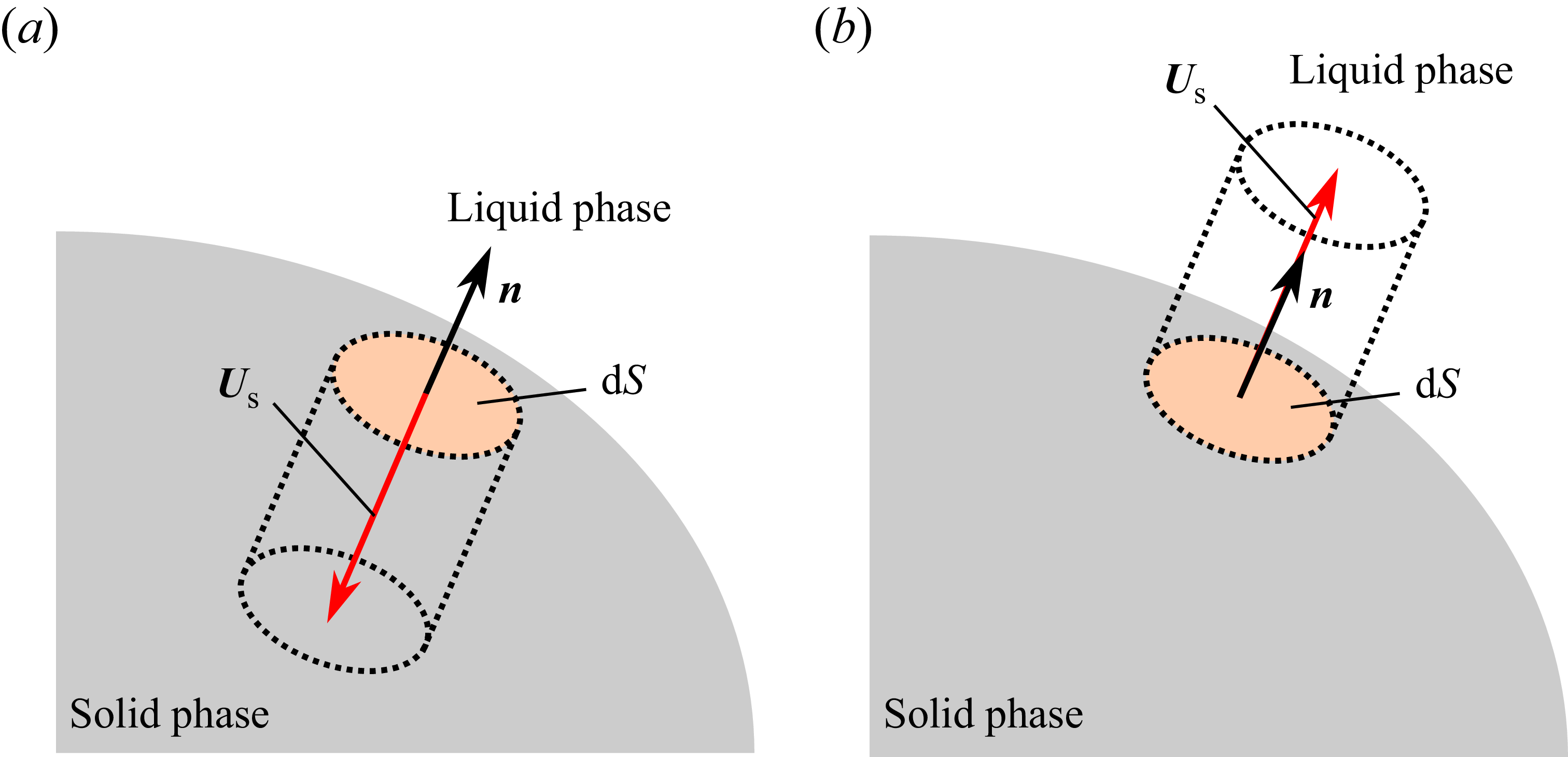
First, we consider the momentum fluxes for melting case. As illustrated in figure 2(a), on an infinitesimal surface element
 $\mathrm{d}S$
, the portion of the solid contained in a columnar region of volume
 $-(\boldsymbol{U}_{\textit{s}} \boldsymbol{\cdot} \boldsymbol{n})\, \mathrm{d}S$
changes per unit time into liquid. Consequently, the momentum contained in this solid-phase region is transferred to the liquid phase, which can be interpreted as the momentum flux due to the Stefan velocity. In addition, due to the volumetric change associated with melting, a jet is induced in the liquid phase as expressed by (2.14); that is, the solid gives a momentum to the liquid by this induced jet. To incorporate both kinds of momentum transfer together, we consider the momentum that the liquid phase obtains and then we consider the momentum that the solid phase obtains as a reaction. During melting, a solid volume of
 $-(\boldsymbol{U}_{\textit{s}} \boldsymbol{\cdot} \boldsymbol{n}) \,\mathrm{d}S$
is changed into a liquid volume of
 $-(\rho _{\textit{b}}/\rho _{\textit{f}}) (\boldsymbol{U}_{\textit{s}} \boldsymbol{\cdot} \boldsymbol{n})\, \mathrm{d}S$
. Since the momentum of the liquid phase per unit volume is
 $\rho _{\textit{f}} \boldsymbol{u}_{\textit{f}}$
, the local momentum that the liquid phase obtains on the surface element
 $\mathrm{d}S$
is expressed as
 \begin{align} \rho _{\textit{f}} \boldsymbol{u}_{\textit{f}} \left (- \frac {\rho _{\textit{b}}}{\rho _{\textit{f}}}\right ) (\boldsymbol{U}_{\textit{s}} \boldsymbol{\cdot} \boldsymbol{n})\,\mathrm{d}S =- \rho _{\textit{b}} \left [ \boldsymbol{u}_{\textit{b}} + \left ( 1-\frac {\rho _{\textit{b}}}{\rho _{\textit{f}}} \right )\boldsymbol{U}_{\textit{s}} \right ] (\boldsymbol{U}_{\textit{s}} \boldsymbol{\cdot} \boldsymbol{n}) \,\mathrm{d}S. \end{align}
Thus, the local momentum that the solid phase obtains, which is the reaction of the above-mentioned momentum transfer, is given by
 \begin{align} \rho _{\textit{b}} \left [ \boldsymbol{u}_{\textit{b}} + \left ( 1-\frac {\rho _{\textit{b}}}{\rho _{\textit{f}}} \right )\boldsymbol{U}_{\textit{s}} \right ] (\boldsymbol{U}_{\textit{s}} \boldsymbol{\cdot} \boldsymbol{n}) \,\mathrm{d}S. \end{align}
Similarly, we can consider the momentum fluxes due to solidification. During solidification, as shown in figure 2(b), a columnar region with a volume of
 $ + (\boldsymbol{U}_{\textit{s}} \boldsymbol{\cdot} \boldsymbol{n}) \,\mathrm{d}S$
changes per unit time into the solid phase on an infinitesimal surface area
 $\mathrm{d}S$
. Thus, due to solidification, a liquid volume of
 $+(\rho _{\textit{b}}/\rho _{\textit{f}}) (\boldsymbol{U}_{\textit{s}} \boldsymbol{\cdot} \boldsymbol{n})\, \mathrm{d}S$
changes into solid and the liquid phase loses momentum. Since the momentum of the liquid phase per unit volume is
 $\rho _{\textit{f}} \boldsymbol{u}_{\textit{f}}$
, the local momentum that the liquid phase loses on the surface element
 $\mathrm{d}S$
is given by
 \begin{align} \rho _{\textit{f}} \boldsymbol{u}_{\textit{f}} \left (+ \frac {\rho _{\textit{b}}}{\rho _{\textit{f}}}\right ) (\boldsymbol{U}_{\textit{s}} \boldsymbol{\cdot} \boldsymbol{n})\,\mathrm{d}S = \rho _{\textit{b}} \left [ \boldsymbol{u}_{\textit{b}} + \left ( 1-\frac {\rho _{\textit{b}}}{\rho _{\textit{f}}} \right )\boldsymbol{U}_{\textit{s}} \right ] (\boldsymbol{U}_{\textit{s}} \boldsymbol{\cdot} \boldsymbol{n})\, \mathrm{d}S. \end{align}
This is equal to the local momentum that the solid phases obtains. Consequently, it takes exactly the same form as the momentum flux that the solid phase obtains during melting given by (3.2).
Columnar region which melts or solidifies in a unit time on an infinitesimal surface area
 $\mathrm{d}S$
of the solid-phase surface
 $\partial {\varOmega }$
: (a) melting with the volume of the columnar region
 $-(\boldsymbol{U}_{\textit{s}} \boldsymbol{\cdot} \boldsymbol{n})\, \mathrm{d}S$
; (b) solidification with the volume of the columnar region
 $+(\boldsymbol{U}_{\textit{s}} \boldsymbol{\cdot} \boldsymbol{n}) \,\mathrm{d}S$
.

From the previous discussion, the net momentum that the solid phase obtains over the solid-phase surface
 $\partial \varOmega$
is given by
 \begin{align} \int _{\partial \varOmega } \rho _{\textit{b}} \left [ \boldsymbol{u}_{\textit{b}} + \left ( 1-\frac {\rho _{\textit{b}}}{\rho _{\textit{f}}} \right )\boldsymbol{U}_{\textit{s}} \right ] (\boldsymbol{U}_{\textit{s}} \boldsymbol{\cdot} \boldsymbol{n}) \,\mathrm{d}S. \end{align}
Therefore, from the conservation law of momentum, the following basic equation of translational motion of the solid phase holds:
 \begin{align} \frac {\mathrm{d}}{\mathrm{d}t}\int _{\varOmega } \rho _{\textit{b}} \boldsymbol{u}_{\textit{b}} \,{\rm d}\boldsymbol{x}^b = \boldsymbol{F} + \int _{\partial \varOmega } \rho _{\textit{b}} \left [ \boldsymbol{u}_{\textit{b}} + \left ( 1-\frac {\rho _{\textit{b}}}{\rho _{\textit{f}}} \right )\boldsymbol{U}_{\textit{s}} \right ] (\boldsymbol{U}_{\textit{s}} \boldsymbol{\cdot} \boldsymbol{n})\, \mathrm{d}S, \end{align}
where
 $\boldsymbol{F}$
is the external force including the fluid force exerted by the ambient liquid phase and the gravitational force, which is expressed in terms of the stress tensor
 $\boldsymbol{\sigma }$
and the gravitational acceleration vector
 $\boldsymbol{G}$
as
 \begin{align} \boldsymbol{F} = \int _{\partial \varOmega } \boldsymbol{\sigma \boldsymbol{\cdot }n}\, \mathrm{d}S + \int _{\varOmega } \rho _{\textit{b}} \boldsymbol{G}\, \mathrm{d}\boldsymbol{x}^b. \end{align}
Since the stress tensor
 $\boldsymbol{\sigma }$
is determined by the pressure and flow velocity in the liquid phase, the flow field of the liquid phase must be known. In this study, however, we do not consider the flow field; instead, the stress tensor
 $\boldsymbol{\sigma }$
is treated as a given quantity. The second term on the right-hand side of (3.5) can be interpreted as the net momentum flux exchanged across the solid surface due to melting and solidification.
By substituting (2.10) into the left-hand side of (3.5), we have
 \begin{align} \frac {\mathrm{d}}{\mathrm{d}t}\int _{\varOmega } \rho _{\textit{b}} \boldsymbol{u}_{\textit{b}}\, \mathrm{d}\boldsymbol{x}^b &= \frac {\mathrm{d}}{\mathrm{d}t}\int _{\varOmega } \rho _{\textit{b}} [\boldsymbol{a}] (\dot {\boldsymbol{R}}^a + \dot {\mathcal{S}}\boldsymbol{x}^b)\, \mathrm{d}\boldsymbol{x}^b \nonumber \\&=[\boldsymbol{a}] \frac {\mathrm{d}}{\mathrm{d}t}\bigg ( \underbrace {\int _{\varOmega } \rho _{\textit{b}}\, \mathrm{d}\boldsymbol{x}^b}_{M} \dot {\boldsymbol{R}}^a + \dot {\mathcal{S}} \underbrace {\int _{\varOmega } \rho _{\textit{b}} \boldsymbol{x}^b \,\mathrm{d}\boldsymbol{x}^b}_{\boldsymbol{Q}^b}\bigg ) \nonumber \\&=[\boldsymbol{a}] \left [ \frac {\mathrm{d}}{\mathrm{d}t}\big(M \dot {\boldsymbol{R}}^a \big) + \frac {\mathrm{d}}{\mathrm{d}t}\big(\dot {\mathcal{S}}\boldsymbol{Q}^b \big)\right ] \nonumber \\&=[\boldsymbol{a}] \big(M \ddot {\boldsymbol{R}}^a + \ddot {\mathcal{S}}\boldsymbol{Q}^b\big) + [\boldsymbol{a}] \big(\dot {M} \dot {\boldsymbol{R}}^a + \dot {\mathcal{S}}\dot {\boldsymbol{Q}}^b \big) \nonumber \\&=[\boldsymbol{a}]\big(M \ddot {\boldsymbol{R}}^a + \ddot {\mathcal{S}}\boldsymbol{Q}^b \big) + \int _{\partial {\varOmega }} \rho _{\textit{b}} \boldsymbol{u}_{\textit{b}} (\boldsymbol{U}_{\textit{s}} \boldsymbol{\cdot} \boldsymbol{n})\,\mathrm{d}S, \end{align}
where, in the final step of the above-mentioned transformation, (2.20) and (2.21) are used to rewrite
 $\dot {M}$
and
 $\dot {\boldsymbol{Q}}^b$
in terms of surface integrals, and (2.10) is then applied to put them together in the form of
 $\boldsymbol{u}_{\textit{b}}$
. The second term on the right-hand side of (3.7) is identical to a part of the second term on the right-hand side of (3.5), and thus they cancel each other out. Finally, by using (A16), the following translational equation of motion is obtained:
 \begin{align} [\boldsymbol{a}]\big \{ M\ddot {\boldsymbol{R}}^a + \mathcal{S} \big [ \boldsymbol{\omega }^b \times (\boldsymbol{\omega }^b \times \boldsymbol{Q}^b) + \dot {\boldsymbol{\omega }}^b \times \boldsymbol{Q}^b \big ]\big \} = \boldsymbol{F} + \int _{\partial \varOmega } \rho _{\textit{b}} \left ( 1-\frac {\rho _{\textit{b}}}{\rho _{\textit{f}}} \right ) \boldsymbol{U}_{\textit{s}} (\boldsymbol{U}_{\textit{s}} \boldsymbol{\cdot} \boldsymbol{n}) \,\mathrm{d}S, \end{align}
where the second term on the right-hand side can be interpreted as the momentum flux by the jet induced in the liquid phase due to density change, and we denote it as
 \begin{align} \boldsymbol{F}_{\textit{s}} = \int _{\partial \varOmega } \rho _{\textit{b}} \left ( 1-\frac {\rho _{\textit{b}}}{\rho _{\textit{f}}} \right ) \boldsymbol{U}_{\textit{s}} (\boldsymbol{U}_{\textit{s}} \boldsymbol{\cdot} \boldsymbol{n}) \,\mathrm{d}S. \end{align}
We can find a similarity between
 $\boldsymbol{F}_{\textit{s}}$
and the jet force in the well-known Tsiolkovsky rocket equation (see Appendix C). In the form independent of the basis vectors, the equation of translational motion is described by
 \begin{align} M\ddot {\boldsymbol{R}} + \boldsymbol{\omega } \times (\boldsymbol{\omega } \times \boldsymbol{Q}) + \dot {\boldsymbol{\omega }} \times \boldsymbol{Q} = \boldsymbol{F} + \boldsymbol{F}_{\textit{s}}, \end{align}
where
 $\boldsymbol{\omega }$
is the angular velocity vector in the form independent of the basis vectors defined by (A17) in Appendix A.4.
3.2. Equation of rotational motion
In this subsection, we derive the equation of the rotational motion of the solid phase, considering the angular momentum fluxes due to phase change.
In the same way as in the previous section, the net angular momentum that the solid phase obtains over the solid-phase surface
 $\partial \varOmega$
is given by
 \begin{align} &\int _{\partial \varOmega } \boldsymbol{r} \times (\rho _{\textit{f}} \boldsymbol{u}_{\textit{f}}) \left (\frac {\rho _{\textit{b}}}{\rho _{\textit{f}}}\right ) (\boldsymbol{U}_{\textit{s}} \boldsymbol{\cdot} \boldsymbol{n})\,\mathrm{d}S \nonumber \\ &=\int _{\partial \varOmega } \rho _{\textit{b}} \boldsymbol{r} \times \left [ \boldsymbol{u}_{\textit{b}} + \left ( 1-\frac {\rho _{\textit{b}}}{\rho _{\textit{f}}} \right )\boldsymbol{U}_{\textit{s}} \right ] (\boldsymbol{U}_{\textit{s}} \boldsymbol{\cdot} \boldsymbol{n})\,\mathrm{d}S \nonumber \\ &=\int _{\partial \varOmega } \rho _{\textit{b}} (\boldsymbol{r} \times \boldsymbol{u}_{\textit{b}}) (\boldsymbol{U}_{\textit{s}} \boldsymbol{\cdot} \boldsymbol{n})\,\mathrm{d}S + \int _{\partial \varOmega } \rho _{\textit{b}} \left ( 1-\frac {\rho _{\textit{b}}}{\rho _{\textit{f}}} \right ) (\boldsymbol{r} \times \boldsymbol{U}_{\textit{s}}) (\boldsymbol{U}_{\textit{s}} \boldsymbol{\cdot} \boldsymbol{n})\,\mathrm{d}S \nonumber \\ &= \int _{\partial \varOmega } \rho _{\textit{b}} (\boldsymbol{r} \times \boldsymbol{u}_{\textit{b}}) (\boldsymbol{U}_{\textit{s}} \boldsymbol{\cdot} \boldsymbol{n})\,\mathrm{d}S + \boldsymbol{R} \times \boldsymbol{F}_{\textit{s}} + \int _{\partial \varOmega } \rho _{\textit{b}} \left ( 1-\frac {\rho _{\textit{b}}}{\rho _{\textit{f}}} \right ) (\boldsymbol{x} \times \boldsymbol{U}_{\textit{s}}) (\boldsymbol{U}_{\textit{s}} \boldsymbol{\cdot} \boldsymbol{n})\,\mathrm{d}S, \end{align}
where, in the final step of the above-mentioned transformation, we have used (2.6) and (3.9). Therefore, from the conservation law of angular momentum about the origin of the
 $[\boldsymbol{a}]$
-frame, the following relation holds:
 \begin{align} &\frac {\mathrm{d}}{\mathrm{d}t}\int _{\varOmega } \boldsymbol{r} \times (\rho _{\textit{b}} \boldsymbol{u}_{\textit{b}})\, \mathrm{d}\boldsymbol{x}^b \nonumber \\ &= \boldsymbol{T}_0 + \boldsymbol{R} \times \boldsymbol{F}_{\textit{s}} + \int _{\partial \varOmega } \rho _{\textit{b}} (\boldsymbol{r} \times \boldsymbol{u}_{\textit{b}}) (\boldsymbol{U}_{\textit{s}} \boldsymbol{\cdot} \boldsymbol{n})\,\mathrm{d}S + \int _{\partial \varOmega } \rho _{\textit{b}} \left ( 1-\frac {\rho _{\textit{b}}}{\rho _{\textit{f}}} \right ) (\boldsymbol{x} \times \boldsymbol{U}_{\textit{s}}) (\boldsymbol{U}_{\textit{s}} \boldsymbol{\cdot} \boldsymbol{n})\,\mathrm{d}S, \end{align}
where
 $\boldsymbol{T}_0$
is the external torque (about the origin of the
 $[\boldsymbol{a}]$
-frame) including the fluid torque exerted by the ambient liquid phase and the gravitational torque, that is,
 \begin{align} \boldsymbol{T}_0 &= \int _{\partial \varOmega } \boldsymbol{r} \times (\boldsymbol{\sigma \boldsymbol{\cdot }n})\, \mathrm{d}S + \int _{\varOmega }\rho _{\textit{b}} \boldsymbol{r} \times \boldsymbol{G} \,\mathrm{d}\boldsymbol{x}^b \nonumber \\ &= \int _{\partial \varOmega } (\boldsymbol{R} + \boldsymbol{x}) \times (\boldsymbol{\sigma \boldsymbol{\cdot }n})\, \mathrm{d}S + \int _{\varOmega }\rho _{\textit{b}} (\boldsymbol{R} + \boldsymbol{x}) \times \boldsymbol{G} \,\mathrm{d}\boldsymbol{x}^b \nonumber \\ &= \boldsymbol{R} \times \underbrace {\left ( \int _{\partial \varOmega } \boldsymbol{\sigma \boldsymbol{\cdot }n} \,\mathrm{d}S + \int _{\varOmega }\rho _{\textit{b}} \boldsymbol{G} \,\mathrm{d}\boldsymbol{x}^b \right )}_{\boldsymbol{F}} + \underbrace {\int _{\partial \varOmega } \boldsymbol{x} \times (\boldsymbol{\sigma \boldsymbol{\cdot }n})\, \mathrm{d}S + \int _{\varOmega }\rho _{\textit{b}} \boldsymbol{x} \times \boldsymbol{G} \,\mathrm{d}\boldsymbol{x}^b}_{\boldsymbol{T}}, \nonumber \\ &= \boldsymbol{R} \times \boldsymbol{F} + \boldsymbol{T}, \end{align}
where
 $\boldsymbol{T}$
denotes the relative torque about the origin of the
 $[\boldsymbol{b}]$
-frame.
By putting (3.12) and (3.13) together, we have the following basic equation of rotational motion of the solid phase:
 \begin{align} &\frac {\mathrm{d}}{\mathrm{d}t}\int _{\varOmega } \boldsymbol{r} \times (\rho _{\textit{b}} \boldsymbol{u}_{\textit{b}})\, \mathrm{d}\boldsymbol{x}^b \nonumber \\ &= \boldsymbol{R} \times (\boldsymbol{F} + \boldsymbol{F}_{\textit{s}}) + \boldsymbol{T} + \int _{\partial \varOmega } \rho _{\textit{b}} (\boldsymbol{r} \times \boldsymbol{u}_{\textit{b}}) (\boldsymbol{U}_{\textit{s}} \boldsymbol{\cdot} \boldsymbol{n})\,\mathrm{d}S \nonumber\\ &\quad + \int _{\partial \varOmega } \rho _{\textit{b}} \left ( 1-\frac {\rho _{\textit{b}}}{\rho _{\textit{f}}} \right ) (\boldsymbol{x} \times \boldsymbol{U}_{\textit{s}}) (\boldsymbol{U}_{\textit{s}} \boldsymbol{\cdot} \boldsymbol{n})\,\mathrm{d}S. \end{align}
By substituting (2.10) into the left-hand side of (3.14), we have
 \begin{align} &\frac {\mathrm{d}}{\mathrm{d}t}\int _{\varOmega } \boldsymbol{r} \times (\rho _{\textit{b}} \boldsymbol{u}_{\textit{b}}) \,\mathrm{d}\boldsymbol{x}^b \nonumber \\[6pt]&= \frac {\mathrm{d}}{\mathrm{d}t}\int _{\varOmega } [\boldsymbol{a}] \rho _{\textit{b}}\left [ \big(\boldsymbol{R}^a + \mathcal{S}\boldsymbol{x}^b \big) \times \big(\dot {\boldsymbol{R}}^a + \dot {\mathcal{S}}\boldsymbol{x}^b \big) \right ]\,\mathrm{d}\boldsymbol{x}^b \nonumber \\[6pt]&=[\boldsymbol{a}] \frac {\mathrm{d}}{\mathrm{d}t}\bigg \{ \bigg ( \underbrace {\int _{\varOmega }\rho _{\textit{b}} \,\mathrm{d}\boldsymbol{x}^b}_{M} \bigg ) \boldsymbol{R}^a \times \dot {\boldsymbol{R}}^a + \boldsymbol{R}^a \times \bigg ( \dot {\mathcal{S}} \underbrace {\int _{\varOmega }\rho _{\textit{b}}\boldsymbol{x}^b\, \mathrm{d}\boldsymbol{x}^b}_{\boldsymbol{Q}^b} \bigg ) \nonumber \\[3pt]&\quad +\bigg ( \mathcal{S} \underbrace {\int _{\varOmega }\rho _{\textit{b}} \boldsymbol{x}^b \,\mathrm{d}\boldsymbol{x}^b}_{\boldsymbol{Q}^b} \bigg ) \times \dot {\boldsymbol{R}}^a + \int _{\varOmega } \rho _{\textit{b}} {\big [ \big(\mathcal{S}\boldsymbol{x}^b \big) \times \big(\dot {\mathcal{S}}\boldsymbol{x}^b \big) \big ]} \,\mathrm{d}\boldsymbol{x}^b \bigg \} \nonumber \\[3pt]&{=[\boldsymbol{a}]\frac {\mathrm{d}}{\mathrm{d}t}\big [ M \boldsymbol{R}^a \times \dot {\boldsymbol{R}}^a + \boldsymbol{R}^a \times \big(\dot {\mathcal{S}} \boldsymbol{Q}^b \big) + \big(\mathcal{S}\boldsymbol{Q}^b \big) \times \dot {\boldsymbol{R}}^a \big ] + [\boldsymbol{a}] \frac {\mathrm{d}}{\mathrm{d}t}\int _{\varOmega } \rho _{\textit{b}} \mathcal{S} \biggl [ \boldsymbol{x}^b \times \big( \underbrace {\mathcal{S}^{\mathrm{T}}\dot {\mathcal{S}}}_{R\big(\boldsymbol{\omega }^b \big)} \boldsymbol{x}^b \big) \biggr ] \,\mathrm{d}\boldsymbol{x}^b } \nonumber \\[3pt]&=[\boldsymbol{a}]\frac {\mathrm{d}}{\mathrm{d}t}\big [ M \boldsymbol{R}^a \times \dot {\boldsymbol{R}}^a + \boldsymbol{R}^a \times \big(\dot {\mathcal{S}} \boldsymbol{Q}^b \big) + \big(\mathcal{S}\boldsymbol{Q}^b \big) \times \dot {\boldsymbol{R}}^a \big ] + [\boldsymbol{a}] \frac {\mathrm{d}}{\mathrm{d}t}\biggl [ \mathcal{S} \int _{\varOmega } \rho _{\textit{b}} R\big(\boldsymbol{x}^b \big)\underbrace {R\big(\boldsymbol{\omega }^b \big)\boldsymbol{x}^b}_{{R\big(\boldsymbol{x}^b \big)^{\mathrm{T}} \boldsymbol{\omega }^b}} \,\mathrm{d}\boldsymbol{x}^b\biggr ] \nonumber \\[3pt]&=[\boldsymbol{a}] \big [\dot {M} \boldsymbol{R}^a \times \dot {\boldsymbol{R}}^a + M \boldsymbol{R}^a \times \ddot {\boldsymbol{R}}^a + \boldsymbol{R}^a \times \big(\ddot {\mathcal{S}} \boldsymbol{Q}^b \big) + \boldsymbol{R}^a \times \big(\dot {\mathcal{S}} \dot {\boldsymbol{Q}}^b \big) + \big(\mathcal{S}\dot {\boldsymbol{Q}}^b \big) \times \dot {\boldsymbol{R}}^a + \big({\mathcal{S}}\boldsymbol{Q}^b \big) \times \ddot {\boldsymbol{R}}^a\big ] \nonumber \\[3pt]&\quad + [\boldsymbol{a}] \frac {\mathrm{d}}{\mathrm{d}t}\bigg [ \mathcal{S} \underbrace {\int _{\varOmega } \rho _{\textit{b}} R\big(\boldsymbol{x}^b \big)R\big(\boldsymbol{x}^b \big)^{\mathrm{T}}\, \mathrm{d}\boldsymbol{x}^b}_{\mathcal{I}^b} \boldsymbol{\omega }^b \bigg ] \nonumber \\[3pt]&=[\boldsymbol{a}] \bigg [ \boldsymbol{R}^a \times \underbrace {\big(M \ddot {\boldsymbol{R}}^a + \ddot {\mathcal{S}}\boldsymbol{Q}^b \big)}_{\boldsymbol{F}^a + \boldsymbol{F}_{\textit{s}}^a}\bigg ] + [\boldsymbol{a}] \big [\big({\mathcal{S}}\boldsymbol{Q}^b \big) \times \ddot {\boldsymbol{R}}^a + \dot {\mathcal{S}}\mathcal{I}^b \boldsymbol{\omega }^b + \mathcal{S} \mathcal{I}^b \dot {\boldsymbol{\omega }}^b \big ] \nonumber \\[3pt]&\quad + [\boldsymbol{a}] \big [ \dot {M} \boldsymbol{R}^a \times \dot {\boldsymbol{R}}^a + \boldsymbol{R}^a \times \big(\dot {\mathcal{S}} \dot {\boldsymbol{Q}}^b \big) + \big(\mathcal{S}\dot {\boldsymbol{Q}}^b \big) \times \dot {\boldsymbol{R}}^a + \mathcal{S}\dot {\mathcal{I}}^b \boldsymbol{\omega }^b \big ], \end{align}
where
 $R(\boldsymbol{\omega }^b)$
is defined by (A14) in Appendix A.4, and (A7), (A10) and (A11) are used in the above-mentioned transformation. By using (2.20)–(2.22) to rewrite
 $\dot {M}$
,
 $\dot {\boldsymbol{Q}}^b$
and
 $\dot {\mathcal{I}}^b$
in terms of surface integrals,
 \begin{align} &{=\boldsymbol{R} \times (\boldsymbol{F}+\boldsymbol{F}_{\textit{s}}) + [\boldsymbol{a}] \big [ \big({\mathcal{S}}\boldsymbol{Q}^b \big) \times \ddot {\boldsymbol{R}}^a + \dot {\mathcal{S}}\mathcal{I}^b \boldsymbol{\omega }^b + \mathcal{S} \mathcal{I}^b \dot {\boldsymbol{\omega }}^b \big ]} \nonumber \\[6pt]&\quad {+ [\boldsymbol{a}] \bigg [ \underbrace {\int _{\partial {\varOmega }} \rho _{\textit{b}} (\boldsymbol{U}_{\textit{s}} \boldsymbol{\cdot } \boldsymbol{n})\, \mathrm{d}S}_{\dot {M}} \boldsymbol{R}^a \times \dot {\boldsymbol{R}}^a + \boldsymbol{R}^a \times \bigg ( \dot {\mathcal{S}} \underbrace {\int _{\partial {\varOmega }} \rho _{\textit{b}} \boldsymbol{x}^b (\boldsymbol{U}_{\textit{s}} \boldsymbol{\cdot } \boldsymbol{n})\, \mathrm{d}S}_{\dot {\boldsymbol{Q}}^b} \bigg )} \nonumber \\[4pt]&\quad \quad {+ \bigg (\mathcal{S} \underbrace {\int _{\partial {\varOmega }} \rho _{\textit{b}} \boldsymbol{x}^b (\boldsymbol{U}_{\textit{s}} \boldsymbol{\cdot } \boldsymbol{n})\, \mathrm{d}S}_{\dot {\boldsymbol{Q}}^b} \bigg ) \times \dot {\boldsymbol{R}}^a + \mathcal{S} \underbrace {\int _{\partial {\varOmega }} \rho _{\textit{b}} R\big(\boldsymbol{x}^b \big)R\big(\boldsymbol{x}^b \big)^{\mathrm{T}} (\boldsymbol{U}_{\textit{s}} \boldsymbol{\cdot } \boldsymbol{n})\, \mathrm{d}S}_{\dot {\mathcal{I}}^b} \boldsymbol{\omega }^b \bigg ] } \nonumber \\[5pt]&{=\boldsymbol{R} \times (\boldsymbol{F}+\boldsymbol{F}_{\textit{s}}) + [\boldsymbol{a}] \big [ \big({\mathcal{S}}\boldsymbol{Q}^b \big) \times \ddot {\boldsymbol{R}}^a + \dot {\mathcal{S}}\mathcal{I}^b \boldsymbol{\omega }^b + \mathcal{S} \mathcal{I}^b \dot {\boldsymbol{\omega }}^b \big ]} \nonumber \\[3pt]&\quad {+ [\boldsymbol{a}] \int _{\partial {\varOmega }} \rho _{\textit{b}} \bigg [\boldsymbol{R}^a \times \dot {\boldsymbol{R}}^a + \boldsymbol{R}^a \times \big(\dot {\mathcal{S}}\boldsymbol{x}^b \big) + \big(\mathcal{S}\boldsymbol{x}^b \big) \times \dot {\boldsymbol{R}}^a + \mathcal{S}R\big(\boldsymbol{x}^b \big)\underbrace {R\big(\boldsymbol{x}^b \big)^{\mathrm{T}} \boldsymbol{\omega }^b}_{\mathcal{S}^{T}\dot {\mathcal{S}} \boldsymbol{x}^b} \bigg ](\boldsymbol{U}_{\textit{s}} \boldsymbol{\cdot } \boldsymbol{n}) \,\mathrm{d}S } \nonumber \\[3pt]&{=\boldsymbol{R} \times (\boldsymbol{F}+\boldsymbol{F}_{\textit{s}}) + [\boldsymbol{a}] \big [ \big({\mathcal{S}}\boldsymbol{Q}^b \big) \times \ddot {\boldsymbol{R}}^a + \dot {\mathcal{S}}\mathcal{I}^b \boldsymbol{\omega }^b + \mathcal{S} \mathcal{I}^b \dot {\boldsymbol{\omega }}^b \big ]} \nonumber \\[3pt]&\quad {+ [\boldsymbol{a}] \int _{\partial {\varOmega }} \rho _{\textit{b}} \bigg [\boldsymbol{R}^a \times \big(\underbrace {\dot {\boldsymbol{R}}^a + \dot {\mathcal{S}}\boldsymbol{x}^b}_{\boldsymbol{u}_{\textit{b}}^a}\big) + \big(\mathcal{S}\boldsymbol{x}^b \big) \times \dot {\boldsymbol{R}}^a + \underbrace {\mathcal{S}R\big(\boldsymbol{x}^b \big)\mathcal{S}^{\mathrm{T}}}_{R\big(\mathcal{S}\boldsymbol{x}^b \big)} \dot {\mathcal{S}} \boldsymbol{x}^b \bigg ](\boldsymbol{U}_{\textit{s}} \boldsymbol{\cdot } \boldsymbol{n})\, \mathrm{d}S } \nonumber \\[3pt]&{=\boldsymbol{R} \times (\boldsymbol{F}+\boldsymbol{F}_{\textit{s}}) + [\boldsymbol{a}] \big [ \big({\mathcal{S}}\boldsymbol{Q}^b \big) \times \ddot {\boldsymbol{R}}^a + \dot {\mathcal{S}}\mathcal{I}^b \boldsymbol{\omega }^b + \mathcal{S} \mathcal{I}^b \dot {\boldsymbol{\omega }}^b \big ]} \nonumber \\[3pt]&\quad {+ [\boldsymbol{a}] \int _{\partial {\varOmega }} \rho _{\textit{b}} \bigg [\boldsymbol{R}^a \times \boldsymbol{u}_{\textit{b}}^a + \big(\mathcal{S}\boldsymbol{x}^b \big) \times \dot {\boldsymbol{R}}^a + \underbrace {R\big(\mathcal{S}\boldsymbol{x}^b \big) \dot {\mathcal{S}} \boldsymbol{x}^b}_{\big(\mathcal{S}\boldsymbol{x}^b \big)\times (\dot {\mathcal{S}} \boldsymbol{x}^b)} \bigg ](\boldsymbol{U}_{\textit{s}} \boldsymbol{\cdot } \boldsymbol{n}) \,\mathrm{d}S } \nonumber \\[3pt]&{=\boldsymbol{R} \times (\boldsymbol{F}+\boldsymbol{F}_{\textit{s}}) + [\boldsymbol{a}] \big [ \big({\mathcal{S}}\boldsymbol{Q}^b \big) \times \ddot {\boldsymbol{R}}^a + \dot {\mathcal{S}}\mathcal{I}^b \boldsymbol{\omega }^b + \mathcal{S} \mathcal{I}^b \dot {\boldsymbol{\omega }}^b \big ]} \nonumber \\[3pt]&\quad {+ [\boldsymbol{a}] \int _{\partial {\varOmega }} \rho _{\textit{b}} \bigg [\boldsymbol{R}^a \times \boldsymbol{u}_{\textit{b}}^a + \big(\mathcal{S}\boldsymbol{x}^b \big) \times (\underbrace {\dot {\boldsymbol{R}}^a + \dot {\mathcal{S}} \boldsymbol{x}^b}_{\boldsymbol{u}_{\textit{b}}^a}) \bigg ] \big(\boldsymbol{U}_{\textit{s}} \boldsymbol{\cdot } \boldsymbol{n} \big)\, \mathrm{d}S } \nonumber \\[3pt]&=\boldsymbol{R} \times (\boldsymbol{F}+\boldsymbol{F}_{\textit{s}}) + [\boldsymbol{a}] \big [ \big({\mathcal{S}}\boldsymbol{Q}^b \big) \times \ddot {\boldsymbol{R}}^a + \dot {\mathcal{S}}\mathcal{I}^b \boldsymbol{\omega }^b + \mathcal{S} \mathcal{I}^b \dot {\boldsymbol{\omega }}^b \big ] + \int _{\partial {\varOmega }} \rho _{\textit{b}} (\boldsymbol{r} \times \boldsymbol{u}_{\textit{b}}) (\boldsymbol{U}_{\textit{s}} \boldsymbol{\cdot} \boldsymbol{n})\,\mathrm{d}S, \end{align}
where (2.7) and (2.10) are applied to put them together in the forms of
 $\boldsymbol{r}$
and
 $\boldsymbol{u}_{\textit{b}}$
in the above-mentioned transformation, respectively. The first term on the right-hand side of (3.16) is identical to the first term on the right-hand side of (3.14), and thus they cancel each other out. In addition, the third term on the right-hand side of (3.16) is identical to the third term on the right-hand side of (3.14), and thus they cancel each other out. Finally, by applying (A15) and (A7) to the remaining terms, and by describing them in the
 $[\boldsymbol{b}]$
-frame, the following rotational equation of motion is obtained:
 \begin{align} [\boldsymbol{b}]\big [ \mathcal{I}^b \dot {\boldsymbol{\omega }}^b + \boldsymbol{\omega }^b \times (\mathcal{I}^b \boldsymbol{\omega }^b) + \boldsymbol{Q}^b \times (\mathcal{S}^{\mathrm{T}} \ddot {\boldsymbol{R}}^a) \big ] = \boldsymbol{T} + \int _{\partial \varOmega } \rho _{\textit{b}} \left ( 1-\frac {\rho _{\textit{b}}}{\rho _{\textit{f}}} \right ) (\boldsymbol{x} \times \boldsymbol{U}_{\textit{s}}) (\boldsymbol{U}_{\textit{s}} \boldsymbol{\cdot} \boldsymbol{n})\, \mathrm{d}S, \end{align}
where the second term on the right-hand side can be interpreted as the angular momentum flux by the jet induced in the liquid phase due to density change, and we denote it as
 \begin{align} \boldsymbol{T}_{\textit{s}} = \int _{\partial \varOmega } \rho _{\textit{b}} \left ( 1-\frac {\rho _{\textit{b}}}{\rho _{\textit{f}}} \right ) (\boldsymbol{x} \times \boldsymbol{U}_{\textit{s}}) (\boldsymbol{U}_{\textit{s}} \boldsymbol{\cdot} \boldsymbol{n})\, \mathrm{d}S. \end{align}
In the form independent of the basis vectors (see also Appendix A.5), the equation of rotational motion is described by
 \begin{align} \mathcal{I} \dot {\boldsymbol{\omega }} + \boldsymbol{\omega } \times (\mathcal{I} \boldsymbol{\omega })+ \boldsymbol{Q} \times \ddot {\boldsymbol{R}} = \boldsymbol{T} + \boldsymbol{T}_{\textit{s}}. \end{align}
4. Discussion
In summary, the derived equations of motion of the solid phase are
 \begin{align} M\ddot {\boldsymbol{R}} + \boldsymbol{\omega } \times (\boldsymbol{\omega } \times \boldsymbol{Q}) + \dot {\boldsymbol{\omega }} \times \boldsymbol{Q} &= \boldsymbol{F} + \boldsymbol{F}_{\textit{s}}, \\[-28pt] \nonumber \end{align}
 \begin{align} \mathcal{I} \dot {\boldsymbol{\omega }} + \boldsymbol{\omega } \times (\mathcal{I} \boldsymbol{\omega }) + \boldsymbol{Q} \times \ddot {\boldsymbol{R}} &= \boldsymbol{T} + \boldsymbol{T}_{\textit{s}}, \\[-12pt] \nonumber \end{align}
where
 $\boldsymbol{F}_{\textit{s}}$
and
 $\boldsymbol{T}_{\textit{s}}$
are the linear and angular momentum fluxes by the jet induced in the liquid phase due to density change, respectively, given by
 \begin{align} \boldsymbol{F}_{\textit{s}} &= \int _{\partial \varOmega } \rho _{\textit{b}} \left ( 1-\frac {\rho _{\textit{b}}}{\rho _{\textit{f}}} \right ) \boldsymbol{U}_{\textit{s}} (\boldsymbol{U}_{\textit{s}} \boldsymbol{\cdot} \boldsymbol{n})\, \mathrm{d}S, \\[-28pt] \nonumber\end{align}
 \begin{align}\boldsymbol{T}_{\textit{s}} &= \int _{\partial \varOmega } \rho _{\textit{b}} \left ( 1-\frac {\rho _{\textit{b}}}{\rho _{\textit{f}}} \right ) (\boldsymbol{x} \times \boldsymbol{U}_{\textit{s}}) (\boldsymbol{U}_{\textit{s}} \boldsymbol{\cdot} \boldsymbol{n})\, \mathrm{d}S. \\[-12pt] \nonumber \end{align}
The mass
 $M$
, mass-moment vector
 $\boldsymbol{Q}$
and inertia tensor
 $\mathcal{I}$
change in time as follows:
 \begin{align}\dot {M} &= \int _{\partial {\varOmega }}\rho _{\textit{b}} (\boldsymbol{U}_{\textit{s}} \boldsymbol{\cdot} \boldsymbol{n})\,\mathrm{d}S,\end{align}
 \begin{align}\dot {\boldsymbol{Q}}^{b} &= \int _{\partial {\varOmega }} \rho _{\textit{b}} \boldsymbol{x}^b (\boldsymbol{U}_{\textit{s}} \boldsymbol{\cdot} \boldsymbol{n}) \,\mathrm{d}S,\end{align}
 \begin{align}\dot {\mathcal{I}}^{b} &= \int _{\partial {\varOmega }} \rho _{\textit{b}} R\big(\boldsymbol{x}^b \big)R\big(\boldsymbol{x}^b \big)^{\mathrm{T}} (\boldsymbol{U}_{\textit{s}} \boldsymbol{\cdot} \boldsymbol{n})\, \mathrm{d}S.\end{align}
Notably,
 $M$
,
 $\boldsymbol{Q}$
and
 $\mathcal{I}$
are time-dependent as shown in the above-mentioned equations. However, in the equations of motion (3.10) and (3.19), the terms including
 $\dot {M}$
,
 $\dot {\boldsymbol{Q}}$
or
 $\dot {\mathcal{I}}$
are not found. These terms have cancelled out a part of the momentum fluxes due to phase change, as seen in the derivations of (3.7) and (3.16). This is consistent with the derivation by Crowe et al. (Reference Crowe, Schwarzkopf, Sommerfeld and Tsuji2011). The remaining part of the fluxes appears as
 $\boldsymbol{F}_{\textit{s}}$
and
 $\boldsymbol{T}_{\textit{s}}$
.
By comparing (3.10) and (3.19) with the conventional rigid-body dynamic equations (1.1) and (1.2), respectively, we find the following two differences.
-
(i) The terms with the mass-moment vector
$\boldsymbol{Q}$
corresponding to the COM are included. -
(ii) The linear and angular momentum fluxes
$\boldsymbol{F}_{\textit{s}}$
and
$\boldsymbol{T}_{\textit{s}}$
by the jet induced in the liquid phase due to density change are included.


In the case of uniform melting and solidification, if the origin of the body-fixed coordinate system is placed at the initial COM, then
 $\boldsymbol{Q} = \boldsymbol{0}$
. Also, owing to symmetry,
 $\boldsymbol{F}_{\textit{s}} = \boldsymbol{0}$
and
 $\boldsymbol{T}_{\textit{s}} = \boldsymbol{0}$
. Therefore, (3.10) and (3.19) reduce to (1.1) and (1.2), respectively, for uniform melting and solidification. In the case of non-uniform melting and solidification, however,
 $\boldsymbol{Q} \neq \boldsymbol{0}$
in general, and the equations of motion should differ from (1.1) and (1.2) due to the effect of item (i). Notably, we cannot eliminate
 $\boldsymbol{Q}$
even when the origin of the
 $[\boldsymbol{b}]$
-frame is adjusted to the COM every instant (see Appendix D). Also, if the density changes,
 $\boldsymbol{F}_{\textit{s}} \neq \boldsymbol{0}$
or
 $\boldsymbol{T}_{\textit{s}} \neq \boldsymbol{0}$
, indicating that the effect of item (ii) appears. Therefore, we have to consider the effects of items (i) and (ii) for non-uniform melting and solidification.
Based on the previous discussion, the answers to questions Q1 and Q2 posed in § 1 are as follows.
-
Answer to question Q1. No, the left-hand side of (1.1) results in
$M {\mathrm{d}\boldsymbol{u}_{\textit{c}}}/{\mathrm{d}t}$
because
$({\mathrm{d}M}/{\mathrm{d}t})\boldsymbol{u}_{\textit{c}}$
cancels out. Instead, the momentum fluxes by the jet induced in the liquid phase due to density change should be included.


-
Answer to question Q2. Yes, the terms representing the effect of the COM shift due to deformation should be included.
5. Conclusions
We considered the system where a solid phase moves in a liquid phase while undergoing melting and solidification, and formulated the equations of motion for the solid phase by using an approach analogous to the derivation of fluid dynamic equations. The momentum flux through the solid-phase surface due to the Stefan velocity is interpreted as the inflow and outflow of momentum across the interface. In addition, the momentum flux by the jet induced in the liquid phase due to density change is also considered. By equating the sum of these momentum fluxes and the external force to the time derivative of the linear momentum of the solid phase, we derived the translational equation of motion. Similarly, by considering the angular momentum balance, we derived the rotational equation of motion. As a result, the derived equations differ formally from the conventional rigid-body dynamic equations owing to the additional flux terms due to density change and the COM shift due to non-uniform deformation.
This study is the first one that theoretically formulates the equations of motion for a solid phase moving in a liquid phase while melting and solidification by integrating the rigid-body dynamics and fluid mechanics. It will be essential in describing the governing equations in numerical simulations for the transport of phase change materials such as ice slurry flows. This study clarifies the differences between the derived equations of motion and the conventional rigid-body dynamic equations, but their significance cannot be evaluated from the theoretical study. It remains for future work using numerical simulations or experiments.
Funding
This work was supported by JSPS KAKENHI grant number JP23H01341.
Declaration of interests
The authors report no conflict of interest.
Appendix A. Notes on algebraic operations and rigid-body kinematics
In this section, we show some notes on algebraic operations and rigid-body kinematics used in §§ 2 and 3. The followings are fundamental concepts on linear algebra and classical mechanics commonly found in standard text books such as that by Goldstein, Poole & Safko (Reference Goldstein, Poole and Safko2002), although the notation used here has been arranged for the purposes of this paper.
A.1 Rotation matrix
A rotational matrix
 $\mathcal{S}$
satisfies
 \begin{align} \mathcal{S}^{\mathrm{T}} = \mathcal{S}^{-1}, \end{align}
 \begin{align} {\det \mathcal{S} = 1}.\\[10pt]\nonumber \end{align}
From (A1), it is proved that
 $\mathcal{S}^{\mathrm{T}}\dot {\mathcal{S}}$
is a skew-symmetric matrix.
A.2 Dot- and cross-products
The dot- and cross-products for two vectors
 $\boldsymbol{x} = [\boldsymbol{a}]\boldsymbol{x}^a = [\boldsymbol{b}]\boldsymbol{x}^b$
and
 $\boldsymbol{y} = [\boldsymbol{a}]\boldsymbol{y}^a = [\boldsymbol{b}]\boldsymbol{y}^b$
(where the notation is common with that in § 2) are defined by
 \begin{align} \boldsymbol{x \boldsymbol{\cdot }y} &= ([\boldsymbol{a}]\boldsymbol{x}^a) \boldsymbol{\cdot } ([\boldsymbol{a}] \boldsymbol{y}^a) = \boldsymbol{x}^a \boldsymbol{\cdot } \boldsymbol{y}^a \\[-9pt] \nonumber\end{align}
 \begin{align} &= ([\boldsymbol{b}]\boldsymbol{x}^b) \boldsymbol{\cdot } ([\boldsymbol{b}] \boldsymbol{y}^b) = \boldsymbol{x}^b \boldsymbol{\cdot } \boldsymbol{y}^b, \\[-9pt] \nonumber\end{align}
 \begin{align} \boldsymbol{x} \times \boldsymbol{y} &= ([\boldsymbol{a}]\boldsymbol{x}^a) \times ([\boldsymbol{a}] \boldsymbol{y}^a) = [\boldsymbol{a}] (\boldsymbol{x}^a \times \boldsymbol{y}^a) \\[-9pt] \nonumber\end{align}
 \begin{align} &= ([\boldsymbol{b}]\boldsymbol{x}^b) \times ([\boldsymbol{b}] \boldsymbol{y}^b) = [\boldsymbol{b}] (\boldsymbol{x}^b \times \boldsymbol{y}^b). \\[10pt] \nonumber\end{align}
Notably, the fact that the same result is obtained in two different coordinate systems is due to the property of the rotation matrix
 $\mathcal{S}$
given in (A1). Note also that (A5) and (A6) can be rewritten as follows:
 \begin{align} \mathcal{S} (\boldsymbol{x}^b \times \boldsymbol{y}^b) = \big(\mathcal{S}\boldsymbol{x}^b \big) \times (\mathcal{S}\boldsymbol{y}^b). \end{align}
A.3 Skew-symmetric matrix
In general, for an arbitrary vector
 $\boldsymbol{A} \in \mathbb{R}^3$
, a corresponding skew-symmetric matrix
 $\mathcal{A}$
can be assigned. This correspondence is defined using the mapping
 $R$
as follows:
 \begin{align} R(\boldsymbol{A}) = \mathcal{A}\ \overset {\mathrm{def}}{\iff }\ R ( \left [ \begin{array}{c} A_1 \\ A_2 \\ A_3 \end{array}\right ] )= \left [ \begin{array}{rrr} 0 & - A_3 & A_2 \\ A_3 & 0 & -A_1 \\ -A_2 & A_1 & 0 \end{array}\right ]. \end{align}
This mapping is a bijective linear map. It also satisfies the following properties for arbitrary vectors
 $\boldsymbol{A}, \,\boldsymbol{B} \in \mathbb{R}^3$
:
 \begin{align} &R(\boldsymbol{A})^{\mathrm{T}} = - R(\boldsymbol{A}),\end{align}
 \begin{align} &R(\boldsymbol{A})\boldsymbol{B} = \boldsymbol{A} \times \boldsymbol{B},\end{align}
 \begin{align} &R(\boldsymbol{A})\boldsymbol{B} = R(\boldsymbol{B})^{\mathrm{T}}\boldsymbol{A},\end{align}
 \begin{align} &R(\mathcal{S}\boldsymbol{A}) = \mathcal{S}R(\boldsymbol{A}) \mathcal{S}^{\mathrm{T}},\end{align}
 \begin{align} &R(\boldsymbol{A})R(\boldsymbol{B})^{\mathrm{T}} = (\boldsymbol{A}\boldsymbol{\cdot }\boldsymbol{B}) \mathcal{E} - \boldsymbol{A}\boldsymbol{B}^{\mathrm{T}},\end{align}
where
 $\mathcal{E}$
is the identity matrix.
A.4 Angular velocity vector
In rigid-body dynamics, the angular velocity vector
 $\boldsymbol{\omega }^b$
observed in the body-fixed coordinate system
 $[\boldsymbol{b}]$
is related to the rotation matrix
 $\mathcal{S}$
as follows:
 \begin{align} R\big(\boldsymbol{\omega }^{b} \big) = \mathcal{S}^{\mathrm{T}} \dot {\mathcal{S}}. \end{align}
From this relation, we have
 \begin{align} \dot {\mathcal{S}} &= \mathcal{S} R\big(\boldsymbol{\omega }^{b} \big), \\[-28pt] \nonumber \end{align}
 \begin{align}\ddot {\mathcal{S}} &= \dot {\mathcal{S}} R\big(\boldsymbol{\omega }^{b} \big) + \mathcal{S} R\big(\dot {\boldsymbol{\omega }}^{b}\big) = \mathcal{S} \big [ R\big(\boldsymbol{\omega }^{b} \big) R\big(\boldsymbol{\omega }^{b} \big) + R\big(\dot {\boldsymbol{\omega }}^{b}\big) \big ] .\\[0pt] \nonumber \end{align}
In the form independent of the basis vectors, the angular velocity vector is denoted by
 \begin{align} \boldsymbol{\omega } = [\boldsymbol{b}] \boldsymbol{\omega }^b. \end{align}
A.5 Description of the form independent of basis vectors
As defined by (2.18), (2.19) and (A17),
 $\mathcal{I}$
and
 $\boldsymbol{\omega }$
are defined in the
 $[\boldsymbol{b}]$
-frame. Consistently, we can define them in the
 $[\boldsymbol{a}]$
-frame as follows:
 \begin{align} &\mathcal{I} = [\boldsymbol{a}] \mathcal{I}^a [\boldsymbol{a}]^{\mathrm{T}},\end{align}
 \begin{align} &\mathcal{I}^a = \int _{\varOmega }\rho _{\textit{b}} R(\boldsymbol{x}^a)R(\boldsymbol{x}^a)^{\mathrm{T}}\, \mathrm{d}\boldsymbol{x}^a,\end{align}
 \begin{align} &\boldsymbol{\omega } = [\boldsymbol{a}] \boldsymbol{\omega }^a,\end{align}
 \begin{align} &\boldsymbol{\omega }^a = \mathcal{S}\boldsymbol{\omega }^b,\end{align}
where
 $\boldsymbol{x}^a = \mathcal{S}\boldsymbol{x}^b$
is the component of the vector
 $\boldsymbol{x}$
in the
 $[\boldsymbol{a}]$
-frame. By comparing (A18) with (2.18), we have
 \begin{align} \mathcal{I}^a &= \mathcal{S} \mathcal{I}^b \mathcal{S}^{\mathrm{T}}. \end{align}
This relation is consistent with (A19) because
 \begin{align} \mathcal{I}^a &= \int _{\varOmega }\rho _{\textit{b}} R(\boldsymbol{x}^a)R(\boldsymbol{x}^a)^{\mathrm{T}} \,\mathrm{d}\boldsymbol{x}^a \nonumber \\ &= \int _{\varOmega }\rho _{\textit{b}} R\big(\mathcal{S}\boldsymbol{x}^b \big)R\big(\mathcal{S}\boldsymbol{x}^b \big)^{\mathrm{T}} \underbrace {\det {\mathcal{S}}}_{1}\, \mathrm{d}\boldsymbol{x}^b \nonumber \\ &= \int _{\varOmega }\rho _{\textit{b}} \left ( \mathcal{S}R\big(\boldsymbol{x}^b \big)\mathcal{S}^{\mathrm{T}} \right ) \left ( \mathcal{S}R\big(\boldsymbol{x}^b \big)\mathcal{S}^{\mathrm{T}} \right )^{\mathrm{T}}\, \mathrm{d}\boldsymbol{x}^b \nonumber \\ &= \mathcal{S} \underbrace {\int _{\varOmega }\rho _{\textit{b}} R\big(\boldsymbol{x}^b \big)R\big(\boldsymbol{x}^b \big)^{\mathrm{T}}\, \mathrm{d}\boldsymbol{x}^b}_{\mathcal{I}^b} \mathcal{S}^{\mathrm{T}}, \end{align}
where (A2) and (A12) are used in the above-mentioned transformation.
By combining (A21) and (A22), we have
 \begin{align} \mathcal{I}^a \boldsymbol{\omega }^a = (\mathcal{S} \mathcal{I}^b \mathcal{S}^{\mathrm{T}}) (\mathcal{S} \boldsymbol{\omega }^b) = \mathcal{S} \mathcal{I}^b \boldsymbol{\omega }^b, \end{align}
which suggests that the vector
 $\mathcal{I}^b \boldsymbol{\omega }^b$
in the
 $[\boldsymbol{b}]$
-frame is mapped to the vector
 $\mathcal{I}^a \boldsymbol{\omega }^a$
in the
 $[\boldsymbol{a}]$
-frame by the function
 $\mathcal{S}$
. Therefore, we can express the vector
 $\mathcal{I} \boldsymbol{\omega }$
as follows:
 \begin{align} \mathcal{I} \boldsymbol{\omega } = [\boldsymbol{b}] \mathcal{I}^b \boldsymbol{\omega }^b = [\boldsymbol{a}] \mathcal{I}^a \boldsymbol{\omega }^a. \end{align}
This equation ensures that the vector
 $\mathcal{I} \boldsymbol{\omega }$
is the form independent of the basis vectors. In addition, the vector
 $\mathcal{I} \dot {\boldsymbol{\omega }}$
is also confirmed to be the form independent of the basis vectors because
 \begin{align} \mathcal{I}^a \dot {\boldsymbol{\omega }}^a &= \mathcal{S} \mathcal{I}^b \mathcal{S}^{\mathrm{T}} \frac {\mathrm{d}}{\mathrm{d}t}(\mathcal{S}\boldsymbol{\omega }^b) \nonumber \\ &=\mathcal{S} \mathcal{I}^b \mathcal{S}^{\mathrm{T}} \left ( \dot {\mathcal{S}}\boldsymbol{\omega }^b + \mathcal{S} \dot {\boldsymbol{\omega }}^b\right ) \nonumber \\ &=\mathcal{S} \mathcal{I}^b \mathcal{S}^{\mathrm{T}} \left( \mathcal{S} \underbrace {R\big(\boldsymbol{\omega }^b \big)\boldsymbol{\omega }^b}_{\boldsymbol{0}} + \mathcal{S} \dot {\boldsymbol{\omega }}^b \right) \nonumber \\ &=\mathcal{S} \mathcal{I}^b \dot {\boldsymbol{\omega }}^b. \end{align}
Appendix B. Formal proof of (2.20)–(2.22)
We derive the time derivatives of the mass (2.20), mass-moment vector (2.21) and inertia tensor (2.22) in § 2.4 from the Leibnitz integral rule.
B.1 Leibnitz integral rule
In general, the Leibnitz integral rule is formulated as follows (Crowe et al. Reference Crowe, Schwarzkopf, Sommerfeld and Tsuji2011):
 \begin{align} \frac {\mathrm{d}}{\mathrm{d}t}\int _{\textit{cv}}f(\boldsymbol{\xi },t)\,\mathrm{d}V = \int _{\textit{cv}}\frac {\partial f(\boldsymbol{\xi },t)}{\partial t}\,\mathrm{d}V + \int _{\textit{cs}} f(\boldsymbol{\xi }, t) (\boldsymbol{u}_{\textit{cs}} \boldsymbol{\cdot} \boldsymbol{n})\, \mathrm{d}S, \end{align}
where
 $f$
is an arbitrary function of the position vector
 $\boldsymbol{\xi }$
(from the origin of the space-fixed coordinate system in
 $\mathbb{R}^3$
) and time
 $t$
, cv denotes an arbitrary control volume, cs denotes the surface of cv,
 $\boldsymbol{n}$
is the normal vector of cs and
 $\boldsymbol{u}_{\textit{cs}}$
is the velocity of cs with respect to the space-fixed coordinate system. Notably, this theorem is described in the space-fixed coordinate system, not in the cv-fixed coordinate system.
In applying the above-mentioned theorem to our system described in § 2, the following correspondence should be considered:
 \begin{align} \begin{cases} {\textit{cv}} = \varOmega , \\ {\textit{cs}} = \partial \varOmega , \\ \boldsymbol{\xi } = \boldsymbol{r}^a = \boldsymbol{R}^a + \mathcal{S}\boldsymbol{x}^b, \\ \mathrm{d}V = \mathrm{d}\boldsymbol{r}^a = \mathrm{d}\boldsymbol{x}^b, \\ \boldsymbol{u}_{\textit{cs}} = \dot {\boldsymbol{r}}^a + \boldsymbol{U}_{\textit{s}}^a = \dot {\boldsymbol{R}}^a + \dot {\mathcal{S}}\boldsymbol{x}^b + \boldsymbol{U}_{\textit{s}}^a. \end{cases} \end{align}
We consider the following three cases corresponding to (2.20)–(2.22):
 \begin{align} f(\boldsymbol{\xi },t) = \begin{cases} \rho _{\textit{b}}, \\ \rho _{\textit{b}}\boldsymbol{r}^a, \\ \rho _{\textit{b}}R(\boldsymbol{r}^a)R(\boldsymbol{r}^a)^{\mathrm{T}}. \end{cases} \end{align}
In the above-mentioned cases,
 $f$
is the function of
 $\boldsymbol{\xi } = \boldsymbol{r}^a$
only, not
 $t$
, and the first term in the right-hand side of (B1) should vanish. Thus, we have
 \begin{align} \frac {\mathrm{d}}{\mathrm{d}t}\int _{\varOmega } f(\boldsymbol{r}^a)\,\mathrm{d}\boldsymbol{r}^a = \int _{\partial \varOmega } f(\boldsymbol{r}^a) \left [\big(\dot {\boldsymbol{r}}^a + \boldsymbol{U}_{\textit{s}}^a \big) \,{\boldsymbol{\cdot }}\, \boldsymbol{n}^a \right ]\, \mathrm{d}S. \end{align}
Notably, we start from (B4) described in the space-fixed coordinate system (
 $[\boldsymbol{a}]$
-frame), although (2.20)–(2.22) are described in the body-fixed coordinate system (
 $[\boldsymbol{b}]$
-frame).
B.2 Derivation of (2.20)
In the first case of (B3), we have the following relation from (B4):
 \begin{align} \frac {\mathrm{d}}{\mathrm{d}t}\int _{\varOmega } \rho _{\textit{b}}\, \mathrm{d}\boldsymbol{r}^a = \int _{\partial \varOmega } \rho _{\textit{b}} \left [(\dot {\boldsymbol{r}}^a + \boldsymbol{U}_{\textit{s}}^a) \,{\boldsymbol{\cdot }}\, \boldsymbol{n}^a \right ]\, \mathrm{d}S. \end{align}
The left-hand side of (B5) is
 \begin{align} \frac {\mathrm{d}}{\mathrm{d}t}\int _{\varOmega } \rho _{\textit{b}} \,\mathrm{d}\boldsymbol{r}^a = \frac {\mathrm{d}}{\mathrm{d}t}\underbrace {\int _{\varOmega } \rho _{\textit{b}} \,\mathrm{d}\boldsymbol{x}^b}_{M} = \dot {M}. \end{align}
The right-hand side of (B5) is
 \begin{align} \int _{\partial \varOmega } \rho _{\textit{b}} \left [\big(\dot {\boldsymbol{r}}^a + \boldsymbol{U}_{\textit{s}}^a \big) {\boldsymbol{\cdot }} \boldsymbol{n}^a \right ] \,{\mathrm{d}}S &=\int _{\partial \varOmega } \rho _{\textit{b}} (\dot {\boldsymbol{r}}^a \boldsymbol{\cdot } \boldsymbol{n}^a) \,{\mathrm{d}}S + \int _{\partial \varOmega } \rho _{\textit{b}} \big(\boldsymbol{U}_{\textit{s}}^a \boldsymbol{\cdot } \boldsymbol{n}^a \big) \,{\mathrm{d}}S \nonumber \\&=\int _{\partial \varOmega } \rho _{\textit{b}} \big [ (\dot {\boldsymbol{R}}^a + \dot {\mathcal{S}}\boldsymbol{x}^b ) \boldsymbol{\cdot } \boldsymbol{n}^a) \big ] {\mathrm{d}}S + \int _{\partial \varOmega } \rho _{\textit{b}} (\boldsymbol{U}_{\textit{s}} \boldsymbol{\cdot } \boldsymbol{n})\, {\mathrm{d}}S \nonumber \\&=\int _{\partial \varOmega } \rho _{\textit{b}} [ (\mathcal{S}^{\mathrm{T}}\dot {\boldsymbol{R}}^a + \underbrace {\mathcal{S}^{\mathrm{T}}\dot {\mathcal{S}}}_{R(\boldsymbol{\omega} ^b)}\boldsymbol{x}^b ) \boldsymbol{\cdot } \boldsymbol{n}^b)]\, {\mathrm{d}}S + \int _{\partial \varOmega } \rho _{\textit{b}} (\boldsymbol{U}_{\textit{s}} \boldsymbol{\cdot } \boldsymbol{n}) \,{\mathrm{d}}S, \end{align}
where
 $\boldsymbol{n}^b = \mathcal{S}^{\mathrm{T}} \boldsymbol{n}^a$
is the component of the normal vector
 $\boldsymbol{n}$
in the
 $[\boldsymbol{b}]$
-frame. We can prove the first term of the right-hand side of (B7) to be zero by using the Gauss’s divergence theorem (shown later). Therefore, (B5) reduces to
 \begin{align} \dot {M} = \int _{\partial \varOmega } \rho _{\textit{b}} (\boldsymbol{U}_{\textit{s}} \boldsymbol{\cdot } \boldsymbol{n}) \,{\mathrm{d}}S. \end{align}
To prove that the first term on the right-hand side of (B7) vanishes, we use tensor notation with the Einstein summation convention, where the subscripts
 $i, \,j, \,k, \,\ldots$
indicate the
 $x, \,y, \,z$
components of a vector or matrix. The superscripts
 $a$
and
 $b$
are omitted in this notation. In the tensor notation, the first term of the right-hand side of (B7) becomes
 \begin{align} \int _{\partial \varOmega } \rho _{\textit{b}} (\mathcal{S}_{ji} \dot {R}_j + \epsilon _{ijk} \omega _{j} x_k) n_i\, {\mathrm{d}}S &= \int _{\varOmega } \frac {\partial }{\partial x_i}\left [ \rho _{\textit{b}} (\mathcal{S}_{ji} \dot {R}_j + \epsilon _{ijk} \omega _{j} x_k) \right ] \mathrm{d}\boldsymbol{x}^b \nonumber \\[4pt] &= \int _{\varOmega } \rho _{\textit{b}} \epsilon _{ijk} \omega _{j} \underbrace {\frac {\partial x_k }{\partial x_i}}_{\delta _{ik}} \,\mathrm{d}\boldsymbol{x}^b \nonumber \\ &= \int _{\varOmega } \rho _{\textit{b}} \underbrace {\epsilon _{kjk}}_{0} \omega _{j}\, \mathrm{d}\boldsymbol{x}^b \nonumber \\ &=0, \end{align}
where
 $\epsilon _{ijk}$
is the Eddington epsilon and
 $\delta _{\textit{ij}}$
is the Kronecker delta.
B.3 Derivation of (2.21)
In the second case of (B3), we have the following relation from (B4):
 \begin{align} \frac {\mathrm{d}}{{\mathrm{d}}t}\int _{\varOmega } \rho _{\textit{b}} \boldsymbol{r}^a \,{\mathrm{d}}\boldsymbol{r}^a = \int _{\partial \varOmega } \rho _{\textit{b}} \boldsymbol{r}^a \left [\big(\dot {\boldsymbol{r}}^a + \boldsymbol{U}_{\textit{s}}^a \big) \, {\boldsymbol{\cdot }}\, \boldsymbol{n}^a \right ] \,{\mathrm{d}}S. \end{align}
The left-hand side of (B10) is
 \begin{align} \frac {\mathrm{d}}{{\mathrm{d}}t}\int _{\varOmega } \rho _{\textit{b}} \boldsymbol{r}^a \,{\mathrm{d}}\boldsymbol{r}^a &= \frac {\mathrm{d}}{{\mathrm{d}}t}\int _{\varOmega } \rho _{\textit{b}} \big(\boldsymbol{R}^a + \mathcal{S}\boldsymbol{x}^b \big) \,{\mathrm{d}}\boldsymbol{x}^b \nonumber \\[4pt] &= \frac {\mathrm{d}}{{\mathrm{d}}t} \Biggl [ \underbrace {\int _{\varOmega } \rho _{\textit{b}} \,{\mathrm{d}}\boldsymbol{x}^b}_{M} \boldsymbol{R}^a + \mathcal{S} \underbrace {\int _{\varOmega } \rho _{\textit{b}} \boldsymbol{x}^b\, {\mathrm{d}}\boldsymbol{x}^b}_{\boldsymbol{Q}^b} \Biggr ] \nonumber \\ &=\frac {\mathrm{d}}{{\mathrm{d}}t} \big ( M\boldsymbol{R}^a + \mathcal{S}\boldsymbol{Q}^b \big ). \end{align}
The right-hand side of (B10) is
 \begin{align} \int _{\partial \varOmega } \rho _{\textit{b}} \boldsymbol{r}^a \left [\big(\dot {\boldsymbol{r}}^a + \boldsymbol{U}_{\textit{s}}^a \big) {\boldsymbol{\cdot }} \boldsymbol{n}^a \right ] \,{\mathrm{d}}S &= \int _{\partial \varOmega } \rho _{\textit{b}} \big(\boldsymbol{R}^a + \mathcal{S}\boldsymbol{x}^b \big) \left [\big(\dot {\boldsymbol{r}}^a + \boldsymbol{U}_{\textit{s}}^a \big) \,{\boldsymbol{\cdot }}\, \boldsymbol{n}^a \right ]\, {\mathrm{d}}S \nonumber \\[4pt]&= \underbrace {\int _{\partial \varOmega } \rho _{\textit{b}} \left [\big(\dot {\boldsymbol{r}}^a + \boldsymbol{U}_{\textit{s}}^a \big) \,{\boldsymbol{\cdot }}\, \boldsymbol{n}^a \right ] \,{\mathrm{d}}S}_{\dot {M}} \boldsymbol{R}^a \nonumber \\&\quad + \mathcal{S} \int _{\partial \varOmega } \rho _{\textit{b}} \boldsymbol{x}^b \left [\big(\dot {\boldsymbol{r}}^a + \boldsymbol{U}_{\textit{s}}^a \big) \,{\boldsymbol{\cdot }}\, \boldsymbol{n}^a \right ] \,{\mathrm{d}}S \nonumber \\&= \dot {M} \boldsymbol{R}^a + \mathcal{S} \int _{\partial \varOmega } \rho _{\textit{b}} \boldsymbol{x}^b [\big(\mathcal{S}^{\mathrm{T}}\dot {\boldsymbol{R}}^a + \underbrace {\mathcal{S}^{\mathrm{T}}\dot {\mathcal{S}}}_{R\big(\boldsymbol{\omega }^b \big) }\boldsymbol{x}^b \big)\boldsymbol{\cdot }\boldsymbol{n}^b] \,{\mathrm{d}}S \nonumber \\&\quad + \mathcal{S} \int _{\partial \varOmega } \rho _{\textit{b}} \boldsymbol{x}^b (\boldsymbol{U}_{\textit{s}} \boldsymbol{\cdot }\boldsymbol{n} ) \,{\mathrm{d}}S, \end{align}
where (2.20) and (B9) are used in the above-mentioned transformation. We can prove that the second term of the right-hand side of (B12) becomes (shown later)
 \begin{align} \mathcal{S} \int _{\partial \varOmega } \rho _{\textit{b}} \boldsymbol{x}^b \big [\big(\mathcal{S}^{\mathrm{T}}\dot {\boldsymbol{R}}^a + R\big(\boldsymbol{\omega }^b \big)\boldsymbol{x}^b \big)\boldsymbol{\cdot }\boldsymbol{n}^b \big ] {\mathrm{d}}S = M\dot {\boldsymbol{R}}^a + \dot {\mathcal{S}} \boldsymbol{Q}^b. \end{align}
Therefore, (B10) reduces to
 \begin{align} &\frac {\mathrm{d}}{{\mathrm{d}}t} \big ( M\boldsymbol{R}^a + \mathcal{S}\boldsymbol{Q}^b \big ) = \dot {M} \boldsymbol{R}^a + M\dot {\boldsymbol{R}}^a + \dot {\mathcal{S}} \boldsymbol{Q}^b + \mathcal{S} \int _{\partial \varOmega } \rho _{\textit{b}} \boldsymbol{x}^b (\boldsymbol{U}_{\textit{s}} \boldsymbol{\cdot }\boldsymbol{n} )\, {\mathrm{d}}S, \nonumber\\[4pt]&\quad \Longrightarrow\, \dot {\boldsymbol{Q}}^{b} = \int _{\partial {\varOmega }} \rho _{\textit{b}} \boldsymbol{x}^b (\boldsymbol{U}_{\textit{s}} \boldsymbol{\cdot} \boldsymbol{n}) \,\mathrm{d}S. \end{align}
To prove (B13), we use the tensor notation again. In the tensor notation, the
 $i$
component of the left-hand side of (B13) becomes
 \begin{align} \mathcal{S}_{\textit{ij}} \int _{\partial \varOmega } \rho _{\textit{b}} x_j (\mathcal{S}_{lk} \dot {R}_l + \epsilon _{klm} \omega _l x_m) n_k \,{\mathrm{d}}S &= \mathcal{S}_{\textit{ij}} \int _{\varOmega } \frac {\partial }{\partial x_k} \left [\rho _{\textit{b}} x_j (\mathcal{S}_{lk} \dot {R}_l + \epsilon _{klm} \omega _l x_m) \right ] \,{\mathrm{d}}\boldsymbol{x}^b \nonumber \\&= \mathcal{S}_{\textit{ij}} \int _{\varOmega } \rho _{\textit{b}} \Biggl [ \underbrace {\frac {\partial x_j}{\partial x_k}}_{\delta _{jk}} (\mathcal{S}_{lk} \dot {R}_l + \epsilon _{klm} \omega _l x_m) + x_j \epsilon _{klm} \omega _l \underbrace {\frac {\partial x_m}{\partial x_k}}_{\delta _{km}} \Biggr ]\, {\mathrm{d}}\boldsymbol{x}^b \nonumber \\&= \mathcal{S}_{\textit{ij}} \int _{\varOmega } \rho _{\textit{b}} \left( \mathcal{S}_{lj} \dot {R}_l + \epsilon _{jlm} \omega _l x_m + x_j \underbrace {\epsilon _{klk}}_{0} \omega _l \right)\, {\mathrm{d}}\boldsymbol{x}^b \nonumber \\&= \int _{\varOmega } \rho _{\textit{b}} ( \underbrace {\mathcal{S}_{\textit{ij}}\mathcal{S}_{lj}}_{\delta _{il}} \dot {R}_l + \underbrace {\mathcal{S}_{\textit{ij}}\epsilon _{jlm} \omega _l}_{\dot {\mathcal{S}}_{im}} x_m )\, {\mathrm{d}}\boldsymbol{x}^b \nonumber \\&= \underbrace {\int _{\varOmega } \rho _{\textit{b}}\, {\mathrm{d}}\boldsymbol{x}^b}_{M} \dot {R}_i + \dot {\mathcal{S}}_{im} \underbrace {\int _{\varOmega } \rho _{\textit{b}} x_m \,{\mathrm{d}}\boldsymbol{x}^b}_{Q_m} \nonumber \\&= \big({M} \dot {\boldsymbol{R}}^a + \dot {\mathcal{S}}\boldsymbol{Q}^b \big)_i, \end{align}
where (A1) and (A15) are used in the above-mentioned transformation.
B.4 Derivation of (2.22)
In the third case of (B3), we have the following relation from (B4):
 \begin{align} \frac {\mathrm{d}}{{\mathrm{d}}t}\int _{\varOmega } \rho _{\textit{b}} R(\boldsymbol{r}^a)R(\boldsymbol{r}^a)^{\mathrm{T}}\, {\mathrm{d}}\boldsymbol{r}^a = \int _{\partial \varOmega } \rho _{\textit{b}} R(\boldsymbol{r}^a)R(\boldsymbol{r}^a)^{\mathrm{T}} \left [\big(\dot {\boldsymbol{r}}^a + \boldsymbol{U}_{\textit{s}}^a \big) \, {\boldsymbol{\cdot }}\, \boldsymbol{n}^a \right ]\, {\mathrm{d}}S. \end{align}
The left-hand side of (B16) is
 \begin{align} &\frac {\mathrm{d}}{{\mathrm{d}}t}\int _{\varOmega } \rho _{\textit{b}} R(\boldsymbol{r}^a)R(\boldsymbol{r}^a)^{\mathrm{T}}\, {\mathrm{d}}\boldsymbol{r}^a \nonumber \\&= \frac {\mathrm{d}}{{\mathrm{d}}t}\int _{\varOmega } \rho _{\textit{b}} R \big(\boldsymbol{R}^a + \mathcal{S}\boldsymbol{x}^b \big)R \big(\boldsymbol{R}^a + \mathcal{S}\boldsymbol{x}^b \big)^{\mathrm{T}} \,{\mathrm{d}}\boldsymbol{x}^b \nonumber \\&= \frac {\mathrm{d}}{{\mathrm{d}}t}\int _{\varOmega } \rho _{\textit{b}} \left [ R(\boldsymbol{R}^a)R(\boldsymbol{R}^a)^{\mathrm{T}} + R(\boldsymbol{R}^a)R\big(\mathcal{S}\boldsymbol{x}^b \big)^{\mathrm{T}} + R\big(\mathcal{S}\boldsymbol{x}^b \big)R(\boldsymbol{R}^a)^{\mathrm{T}} + R\big(\mathcal{S}\boldsymbol{x}^b \big)R\big(\mathcal{S}\boldsymbol{x}^b \big)^{\mathrm{T}}\right ] \,{\mathrm{d}}\boldsymbol{x}^b \nonumber \\&= \frac {\mathrm{d}}{{\mathrm{d}}t}\Biggl [ \underbrace {\int _{\varOmega } \rho _{\textit{b}} \,{\mathrm{d}}\boldsymbol{x}^b}_{M} R(\boldsymbol{R}^a)R(\boldsymbol{R}^a)^{\mathrm{T}} + R(\boldsymbol{R}^a)R (\mathcal{S}\underbrace {\int _{\varOmega } \rho _{\textit{b}}\boldsymbol{x}^b \,{\mathrm{d}}\boldsymbol{x}^b}_{\boldsymbol{Q}^b})^{\mathrm{T}} + R(\mathcal{S}\underbrace {\int _{\varOmega } \rho _{\textit{b}}\boldsymbol{x}^b \,{\mathrm{d}}\boldsymbol{x}^b}_{\boldsymbol{Q}^b})R(\boldsymbol{R}^a)^{\mathrm{T}} \nonumber \\&\quad \quad \quad \quad \quad + \int _{\varOmega } \rho _{\textit{b}}\underbrace {R\big(\mathcal{S}\boldsymbol{x}^b \big)}_{\mathcal{S}R\big(\boldsymbol{x}^b \big)\mathcal{S}^{\mathrm{T}}}\underbrace {R\big(\mathcal{S}\boldsymbol{x}^b \big)^{\mathrm{T}}}_{\mathcal{S}R\big(\boldsymbol{x}^b \big)^{\mathrm{T}}\mathcal{S}^{\mathrm{T}}}\, {\mathrm{d}}\boldsymbol{x}^b \Biggr ] \nonumber \\&= \frac {\mathrm{d}}{{\mathrm{d}}t}\Biggl [ {M} R(\boldsymbol{R}^a)R(\boldsymbol{R}^a)^{\mathrm{T}} + R(\boldsymbol{R}^a)R(\mathcal{S}\boldsymbol{Q}^b)^{\mathrm{T}} + R(\mathcal{S}\boldsymbol{Q}^b)R(\boldsymbol{R}^a)^{\mathrm{T}} + \mathcal{S} \underbrace {\int _{\varOmega } \rho _{\textit{b}} R\big(\boldsymbol{x}^b \big) R\big(\boldsymbol{x}^b \big)^{\mathrm{T}} \,{\mathrm{d}}\boldsymbol{x}^b}_{\mathcal{I}^b} \mathcal{S}^{\mathrm{T}} \Biggr ] \nonumber \\&= \frac {\mathrm{d}}{{\mathrm{d}}t}\left [ {M} R(\boldsymbol{R}^a)R(\boldsymbol{R}^a)^{\mathrm{T}} + R(\boldsymbol{R}^a)R(\mathcal{S}\boldsymbol{Q}^b)^{\mathrm{T}} + R(\mathcal{S}\boldsymbol{Q}^b)R(\boldsymbol{R}^a)^{\mathrm{T}} + \mathcal{S} \mathcal{I}^b \mathcal{S}^{\mathrm{T}} \right ], \end{align}
where the linearity of the function
 $R$
and (A12) are used in the above-mentioned transformation. The right-hand side of (B16) is
 \begin{align} &\int _{\partial \varOmega } \rho _{\textit{b}} R(\boldsymbol{r}^a)R(\boldsymbol{r}^a)^{\mathrm{T}} \left [(\dot {\boldsymbol{r}}^a + \boldsymbol{U}_{\textit{s}}^a) \,{\boldsymbol{\cdot }}\, \boldsymbol{n}^a \right ]\, {\mathrm{d}}S \nonumber \\&= \int _{\partial \varOmega } \rho _{\textit{b}} R(\boldsymbol{R}^a + \mathcal{S}\boldsymbol{x}^b)R(\boldsymbol{R}^a + \mathcal{S}\boldsymbol{x}^b)^{\mathrm{T}} \left [(\dot {\boldsymbol{r}}^a + \boldsymbol{U}_{\textit{s}}^a)\, {\boldsymbol{\cdot }}\, \boldsymbol{n}^a \right ]\, {\mathrm{d}}S \nonumber \\&= \int _{\partial \varOmega } \rho _{\textit{b}} \left [ R(\boldsymbol{R}^a)R(\boldsymbol{R}^a)^{\mathrm{T}} + R(\boldsymbol{R}^a)R(\mathcal{S}\boldsymbol{x}^b)^{\mathrm{T}} + R(\mathcal{S}\boldsymbol{x}^b)R(\boldsymbol{R}^a)^{\mathrm{T}} + R(\mathcal{S}\boldsymbol{x}^b)R(\mathcal{S}\boldsymbol{x}^b)^{\mathrm{T}}\right ] \left [(\dot {\boldsymbol{r}}^a + \boldsymbol{U}_{\textit{s}}^a) \,{\boldsymbol{\cdot }}\, \boldsymbol{n}^a \right ]\, {\mathrm{d}}S \nonumber \\&= \underbrace {\int _{\partial \varOmega } \rho _{\textit{b}} \left [(\dot {\boldsymbol{r}}^a + \boldsymbol{U}_{\textit{s}}^a) {\boldsymbol{\cdot }} \boldsymbol{n}^a \right ] {\mathrm{d}}S}_{\dot {M}} R(\boldsymbol{R}^a)R(\boldsymbol{R}^a)^{\mathrm{T}} + R(\boldsymbol{R}^a)R(\underbrace {\mathcal{S}\int _{\partial \varOmega } \rho _{\textit{b}}\boldsymbol{x}^b\left [(\dot {\boldsymbol{r}}^a + \boldsymbol{U}_{\textit{s}}^a) \, {\boldsymbol{\cdot }}\, \boldsymbol{n}^a \right ]\, {\mathrm{d}}S}_{M\dot {\boldsymbol{R}}^{a} + \dot {\mathcal{S}}\boldsymbol{Q}^b + \mathcal{S}\dot {\boldsymbol{Q}}^b})^{\mathrm{T}} \nonumber \\&\ + R( \underbrace {\mathcal{S} \int _{\partial \varOmega } \rho _{\textit{b}}\boldsymbol{x}^b\left [(\dot {\boldsymbol{r}}^a + \boldsymbol{U}_{\textit{s}}^a) {\boldsymbol{\cdot }} \boldsymbol{n}^a \right ] \,{\mathrm{d}}S}_{M\dot {\boldsymbol{R}}^{a} + \dot {\mathcal{S}}\boldsymbol{Q}^b + \mathcal{S}\dot {\boldsymbol{Q}}^b}) R(\boldsymbol{R}^a)^{\mathrm{T}} + \mathcal{S} \int _{\partial \varOmega } \rho _{\textit{b}} R(\boldsymbol{x}^b)R(\boldsymbol{x}^b)^{\mathrm{T}} \left [(\dot {\boldsymbol{r}}^a + \boldsymbol{U}_{\textit{s}}^a) \,{\boldsymbol{\cdot }}\, \boldsymbol{n}^a \right ] {\mathrm{d}}S \mathcal{S}^{\mathrm{T}} \nonumber \\&= \dot {M} R(\boldsymbol{R}^a)R(\boldsymbol{R}^a)^{\mathrm{T}} + R(\boldsymbol{R}^a)R(M\dot {\boldsymbol{R}}^{a} + \frac {\mathrm{d}}{{\mathrm{d}} t} (\mathcal{S}\boldsymbol{Q}^b))^{\mathrm{T}} + R(M\dot {\boldsymbol{R}}^{a} + \frac {\mathrm{d}}{{\mathrm{d}} t} (\mathcal{S}\boldsymbol{Q}^b)) R(\boldsymbol{R}^a)^{\mathrm{T}} \nonumber \\&\ + \mathcal{S} \int _{\partial \varOmega } \rho _{\textit{b}} R(\boldsymbol{x}^b)R(\boldsymbol{x}^b)^{\mathrm{T}} [(\mathcal{S}^{\mathrm{T}} \dot {\boldsymbol{R}}^a + \underbrace {\mathcal{S}^{\mathrm{T}}\dot {\mathcal{S}}}_{R(\boldsymbol{\omega }^b)} \boldsymbol{x}^b ) \boldsymbol{\cdot } \boldsymbol{n}^b ]\, {\mathrm{d}}S \mathcal{S}^{\mathrm{T}} + \mathcal{S} \int _{\partial \varOmega } \rho _{\textit{b}} R(\boldsymbol{x}^b)R(\boldsymbol{x}^b)^{\mathrm{T}} (\boldsymbol{U}_{\textit{s}} \boldsymbol{\cdot } \boldsymbol{n}) \,{\mathrm{d}}S \mathcal{S}^{\mathrm{T}} \nonumber \\&= \frac {\mathrm{d}}{{\mathrm{d}}t}\big({M} R(\boldsymbol{R}^a)R(\boldsymbol{R}^a)^{\mathrm{T}}\big) + R(\boldsymbol{R}^a)R \left(\frac {\mathrm{d}}{{\mathrm{d}} t} (\mathcal{S}\boldsymbol{Q}^b)\right)^{\mathrm{T}} + R \left(\frac {\mathrm{d}}{{\mathrm{d}} t} (\mathcal{S}\boldsymbol{Q}^b)\right) R(\boldsymbol{R}^a)^{\mathrm{T}} \nonumber \\&\ + \mathcal{S} \int _{\partial \varOmega } \rho _{\textit{b}} R(\boldsymbol{x}^b)R(\boldsymbol{x}^b)^{\mathrm{T}} \big[\big(\mathcal{S}^{\mathrm{T}} \dot {\boldsymbol{R}}^a + R(\boldsymbol{\omega }^b) \boldsymbol{x}^b \big) \boldsymbol{\cdot } \boldsymbol{n}^b \big]\, {\mathrm{d}}S \mathcal{S}^{\mathrm{T}} + \mathcal{S} \int _{\partial \varOmega } \rho _{\textit{b}} R(\boldsymbol{x}^b)R\big(\boldsymbol{x}^b \big)^{\mathrm{T}} (\boldsymbol{U}_{\textit{s}} \boldsymbol{\cdot } \boldsymbol{n}) \,{\mathrm{d}}S \mathcal{S}^{\mathrm{T}}, \end{align}
where (2.20), (B9), (2.21) and (B13) are used in the above-mentioned transformation. We can prove that the forth term of the right-hand side of (B18) becomes (shown later)
 \begin{align} &\mathcal{S} \int _{\partial \varOmega } \rho _{\textit{b}} R\big(\boldsymbol{x}^b \big)R\big(\boldsymbol{x}^b \big)^{\mathrm{T}} \big[(\mathcal{S}^{\mathrm{T}} \dot {\boldsymbol{R}}^a + R\big(\boldsymbol{\omega }^b \big) \boldsymbol{x}^b ) \boldsymbol{\cdot } \boldsymbol{n}^b \big]\, {\mathrm{d}}S \mathcal{S}^{\mathrm{T}} \nonumber\\&\quad= R(\mathcal{S}\boldsymbol{Q}^b)R(\dot {\boldsymbol{R}}^a)^{\mathrm{T}} + R(\dot {\boldsymbol{R}}^a)R(\mathcal{S}\boldsymbol{Q}^b)^{\mathrm{T}} + \dot {\mathcal{S}}\mathcal{I}^b \mathcal{S}^{\mathrm{T}} + {\mathcal{S}}\mathcal{I}^b \dot {\mathcal{S}}^{\mathrm{T}}. \end{align}
Therefore, (B16) reduces to
 \begin{align} &\frac {\mathrm{d}}{{\mathrm{d}}t}\left [ {M} R(\boldsymbol{R}^a)R(\boldsymbol{R}^a)^{\mathrm{T}} + R(\boldsymbol{R}^a)R(\mathcal{S}\boldsymbol{Q}^b)^{\mathrm{T}} + R(\mathcal{S}\boldsymbol{Q}^b)R(\boldsymbol{R}^a)^{\mathrm{T}} + \mathcal{S} \mathcal{I}^b \mathcal{S}^{\mathrm{T}} \right ] \nonumber \\ &= \frac {\mathrm{d}}{{\mathrm{d}}t}({M} R(\boldsymbol{R}^a)R(\boldsymbol{R}^a)^{\mathrm{T}}) + R(\boldsymbol{R}^a)R(\frac {\mathrm{d}}{{\mathrm{d}} t} (\mathcal{S}\boldsymbol{Q}^b))^{\mathrm{T}} + R(\frac {\mathrm{d}}{{\mathrm{d}} t} (\mathcal{S}\boldsymbol{Q}^b)) R(\boldsymbol{R}^a)^{\mathrm{T}} \nonumber \\ &\ + R(\mathcal{S}\boldsymbol{Q}^b)R(\dot {\boldsymbol{R}}^a)^{\mathrm{T}} + R(\dot {\boldsymbol{R}}^a)R(\mathcal{S}\boldsymbol{Q}^b)^{\mathrm{T}} + \dot {\mathcal{S}}\mathcal{I}^b \mathcal{S}^{\mathrm{T}} + {\mathcal{S}}\mathcal{I}^b \dot {\mathcal{S}}^{\mathrm{T}}\nonumber\\&\quad +\mathcal{S} \int _{\partial \varOmega } \rho _{\textit{b}} R\big(\boldsymbol{x}^b \big)R\big(\boldsymbol{x}^b \big)^{\mathrm{T}} (\boldsymbol{U}_{\textit{s}} \boldsymbol{\cdot } \boldsymbol{n})\, {\mathrm{d}}S \mathcal{S}^{\mathrm{T}},\nonumber\\[5pt] &\quad \Longrightarrow\, \dot {\mathcal{I}}^{b} = \int _{\partial {\varOmega }} \rho _{\textit{b}} R\big(\boldsymbol{x}^b \big)R\big(\boldsymbol{x}^b \big)^{\mathrm{T}} (\boldsymbol{U}_{\textit{s}} \boldsymbol{\cdot} \boldsymbol{n})\, \mathrm{d}S.\end{align}
Finally, we prove (B19) using the tensor notation. The
 $ij$
component of the left-hand side of (B19) becomes

where (A1), (A15), (A13) and the skey-symmetry of
 $\mathcal{S}\dot {\mathcal{S}}^{\mathrm{T}}$
are used in the above-mentioned transformation.
Appendix C. Derivation of Tsiolkovsky rocket equation
As a verification of the derived equations, we consider a well-known problem similar to the present system, i.e. the rigid body dynamics of a rocket that is moving in space while losing mass due to combustion of fuel.
We consider a rocket
 $\varOmega$
composed of a vehicle part (including a payload)
 $\varOmega _{\textit{a}}$
and a fuel part
 $\varOmega _{\textit{b}}$
. These parts move together as a rigid body, but the fuel part
 $\varOmega _{\textit{b}}$
loses its mass due to combustion of fuel. In the same way as § 2, let the
 $[\boldsymbol{a}]$
- and
 $[\boldsymbol{b}]$
-frames be the coordinate systems fixed to the space and to
 $\varOmega$
, respectively. Let the velocity of
 $\partial \varOmega _{\textit{b}}$
with respect to the
 $[\boldsymbol{b}]$
-frame be
 $\boldsymbol{U}_{\textit{s}}$
, representing the local mass loss of the fuel part
 $\varOmega _{\textit{b}}$
. The mass lost from
 $\varOmega _{\textit{b}}$
becomes an exhaust gas and is ejected through
 $\partial \varOmega _{\textit{b}}$
into outer space with velocity
 $\boldsymbol{W}$
relative to the
 $[\boldsymbol{b}]$
-frame. Let the densities of
 $\varOmega _{\textit{a}}$
,
 $\varOmega _{\textit{b}}$
and the exhaust gas be
 $\rho _{\textit{a}}$
,
 $\rho _{\textit{b}}$
and
 $\rho _{\textit{f}}$
, respectively.
At first, the mass
 $M$
of the rocket is given by
 \begin{align} M = \underbrace {\int _{\varOmega _{\textit{a}}} \rho _{\textit{a}} \,\mathrm{d}\boldsymbol{x}^b}_{M_{\textit{a}}} + \underbrace {\int _{\varOmega _{\textit{b}}} \rho _{\textit{b}} \,\mathrm{d}\boldsymbol{x}^b}_{M_{\textit{b}}}, \end{align}
where
 $M_{\textit{a}}$
and
 $M_{\textit{b}}$
are the masses of
 $\varOmega _{\textit{a}}$
and
 $\varOmega _{\textit{b}}$
, respectively. The time derivative of
 $M$
is given in the same way as (2.20) by
 \begin{align} \dot {M} = \dot {M}_{\textit{b}} = \int _{\partial {\varOmega _{\textit{b}}}}\rho _{\textit{b}} (\boldsymbol{U}_{\textit{s}} \boldsymbol{\cdot} \boldsymbol{n})\,\mathrm{d}S. \end{align}
Note that the integral in the right-hand side of (C2) is over
 $\partial {\varOmega }_{\textit{b}}$
only. Similarly, the mass-moment vector
 $\boldsymbol{Q}^b$
in the
 $[\boldsymbol{b}]$
-frame is given by
 \begin{align} \boldsymbol{Q}^b = \underbrace {\int _{{\varOmega }_{\textit{a}}}\rho _{\textit{a}} \boldsymbol{x}^{b} \,\mathrm{d}\boldsymbol{x}^{b}}_{\boldsymbol{Q}^b_{\textit{a}}} + \underbrace {\int _{{\varOmega }_{\textit{b}}}\rho _{\textit{b}} \boldsymbol{x}^{b}\, \mathrm{d}\boldsymbol{x}^{b}}_{\boldsymbol{Q}^b_{\textit{b}}}, \end{align}
where
 $\boldsymbol{Q}^b_{\textit{a}}$
and
 $\boldsymbol{Q}^b_{\textit{b}}$
are the mass-moment vectors of
 $\varOmega _{\textit{a}}$
and
 $\varOmega _{\textit{b}}$
, respectively. The time derivative of
 $\boldsymbol{Q}^b$
is given in the same way as (2.21) by
 \begin{align} \dot {\boldsymbol{Q}}^{b} = \dot {\boldsymbol{Q}}_{\textit{b}}^{b} = \int _{\partial {\varOmega }_{\textit{b}}} \rho _{\textit{b}} \boldsymbol{x}^b (\boldsymbol{U}_{\textit{s}} \boldsymbol{\cdot} \boldsymbol{n})\, \mathrm{d}S. \end{align}
Note again that the integral in the right-hand side of (C4) is over
 $\partial {\varOmega }_{\textit{b}}$
only. Also,
 $M_{\textit{a}}$
and
 $\boldsymbol{Q}^b_{\textit{a}}$
are time-independent, whereas
 $M_{\textit{b}}$
and
 $\boldsymbol{Q}^b_{\textit{b}}$
are time-dependent.
The velocity
 $\boldsymbol{u}_{\textit{b}}$
of an arbitrary point in
 $\varOmega$
(including both
 $\varOmega _{\textit{a}}$
and
 $\varOmega _{\textit{b}}$
) is equal to (2.10), i.e.
 \begin{align} \boldsymbol{u}_{\textit{b}} = [\boldsymbol{a}](\dot {\boldsymbol{R}}^a + \dot {\mathcal{S}}\boldsymbol{x}^b). \end{align}
The velocity
 $\boldsymbol{u}_{\textit{f}}$
of the exhaust gas with respect to the
 $[\boldsymbol{a}]$
-frame is given by
 \begin{align} \boldsymbol{u}_{\textit{f}} = \boldsymbol{u}_{\textit{b}} + \boldsymbol{W}\quad (\text{on}\,\partial {\varOmega }_{\textit{b}}). \end{align}
Note that the jet due to combustion
 $\boldsymbol{W}$
replaces the jet due to density change
 $(1-\rho _{\textit{b}}/\rho _{\textit{f}})\boldsymbol{U}_{\textit{s}}$
in (2.14).
We consider the momentum that the exhaust gas obtains and then we consider the momentum that the rocket obtains as a reaction. Due to combustion, a portion of
 $\varOmega _{\textit{b}}$
with a volume of
 $-(\boldsymbol{U}_{\textit{s}} \boldsymbol{\cdot} \boldsymbol{n})\, \mathrm{d}S$
is changed into an exhaust gas with a volume of
 $-(\rho _{\textit{b}}/\rho _{\textit{f}}) (\boldsymbol{U}_{\textit{s}} \boldsymbol{\cdot} \boldsymbol{n})\, \mathrm{d}S$
. Since the momentum of the exhaust gas per unit volume is
 $\rho _{\textit{f}} \boldsymbol{u}_{\textit{f}}$
, the local momentum that the exhaust gas obtains on the surface element
 $\mathrm{d}S$
on
 $\varOmega _{\textit{b}}$
is expressed as
 \begin{align} \rho _{\textit{f}} \boldsymbol{u}_{\textit{f}} \left (- \frac {\rho _{\textit{b}}}{\rho _{\textit{f}}}\right ) (\boldsymbol{U}_{\textit{s}} \boldsymbol{\cdot} \boldsymbol{n})\,\mathrm{d}S =- \rho _{\textit{b}} ( \boldsymbol{u}_{\textit{b}} + \boldsymbol{W}) (\boldsymbol{U}_{\textit{s}} \boldsymbol{\cdot} \boldsymbol{n}) \,\mathrm{d}S. \end{align}
Thus, the local momentum that
 $\varOmega _{\textit{b}}$
obtains, which is the reaction of the above-mentioned momentum transfer, is given by
 \begin{align} \rho _{\textit{b}} ( \boldsymbol{u}_{\textit{b}} + \boldsymbol{W}) (\boldsymbol{U}_{\textit{s}} \boldsymbol{\cdot} \boldsymbol{n}) \,\mathrm{d}S. \end{align}
Thus, the net momentum that
 $\varOmega _{\textit{b}}$
obtains over
 $\partial \varOmega _{\textit{b}}$
is given by
 \begin{align} \int _{\partial \varOmega _{\textit{b}}} \rho _{\textit{b}} ( \boldsymbol{u}_{\textit{b}} + \boldsymbol{W}) (\boldsymbol{U}_{\textit{s}} \boldsymbol{\cdot} \boldsymbol{n})\, \mathrm{d}S. \end{align}
Therefore, from the conservation law of momentum, the rocket equation holds as follows:
 \begin{align} \frac {\mathrm{d}}{\mathrm{d}t}\left [ \int _{\varOmega _{\textit{a}}} \rho _{\textit{a}} \boldsymbol{u}_{\textit{b}}\, {\rm d}\boldsymbol{x}^b + \int _{\varOmega _{\textit{b}}} \rho _{\textit{b}} \boldsymbol{u}_{\textit{b}} \,{\rm d}\boldsymbol{x}^b \right ] = \int _{\partial \varOmega _{\textit{b}}} \rho _{\textit{b}} (\boldsymbol{u}_{\textit{b}} + \boldsymbol{W}) (\boldsymbol{U}_{\textit{s}} \boldsymbol{\cdot} \boldsymbol{n})\, \mathrm{d}S, \end{align}
where the external force does not appear because the rocket moves in space. In the same way as in (3.7), the left-hand side of (C10) becomes
 \begin{align} \frac {\mathrm{d}}{\mathrm{d}t}\left [ \int _{\varOmega _{\textit{a}}} \rho _{\textit{a}} \boldsymbol{u}_{\textit{b}} \,{\rm d}\boldsymbol{x}^b + \int _{\varOmega _{\textit{b}}} \rho _{\textit{b}} \boldsymbol{u}_{\textit{b}} \,{\rm d}\boldsymbol{x}^b \right ] &= [\boldsymbol{a}]\Bigl [ (\underbrace {M_{\textit{a}} + M_{\textit{b}}}_{M})\ddot {\boldsymbol{R}}^a + \ddot {\mathcal{S}}(\underbrace {\boldsymbol{Q}^b_{\textit{a}} + \boldsymbol{Q}^b_{\textit{b}}}_{\boldsymbol{Q}^b})\Bigr ] \nonumber\\&\quad+ \int _{\partial {\varOmega }_{\textit{b}}} \rho _{\textit{b}} \boldsymbol{u}_{\textit{b}} (\boldsymbol{U}_{\textit{s}} \boldsymbol{\cdot} \boldsymbol{n})\,\mathrm{d}S, \end{align}
where (C2) and (C4) are used in the above-mentioned transformation. The second term on the right-hand side of (C11) is identical to a part of the second term on the right-hand side of (C10), and thus they cancel each other out. Finally, we have
 \begin{align} [\boldsymbol{a}]\left \{ M\ddot {\boldsymbol{R}}^a + \mathcal{S} \left [ \boldsymbol{\omega }^b \times (\boldsymbol{\omega }^b \times \boldsymbol{Q}^b) + \dot {\boldsymbol{\omega }}^b \times \boldsymbol{Q}^b \right ]\right \} = \int _{\partial \varOmega _{\textit{b}}} \rho _{\textit{b}} \boldsymbol{W} (\boldsymbol{U}_{\textit{s}} \boldsymbol{\cdot} \boldsymbol{n})\, \mathrm{d}S. \end{align}
The right-hand side of (C12) represents the jet force of the rocket, which corresponds to
 $\boldsymbol{F}_{\textit{s}}$
in (3.10).
To see the consistency with the well-known Tsiolkovsky rocket equation, we consider the one-dimensional motion where
 \begin{align} \dot {\boldsymbol{R}}^a = \left [ \begin{array}{c} V \\ 0 \\ 0 \end{array} \right ],\quad \boldsymbol{\omega }^b = \boldsymbol{0},\quad \boldsymbol{W}^a = \left [ \begin{array}{c} - w \\ 0 \\ 0 \end{array} \right ], \end{align}
where
 $w$
is constant. In this situation, (C12) becomes
 \begin{align} M\dot {V} = \int _{\varOmega _{\textit{b}}} \rho _{\textit{b}} (-w) (\boldsymbol{U}_{\textit{s}}\boldsymbol{\cdot }\boldsymbol{n})\,\mathrm{d}S = - w \underbrace {\int _{\varOmega _{\textit{b}}} \rho _{\textit{b}}(\boldsymbol{U}_{\textit{s}}\boldsymbol{\cdot }\boldsymbol{n})\,\mathrm{d}S}_{\dot {M}} = - w \dot {M}. \end{align}
Therefore, the Tsiolkovsky rocket equation is derived as follows:
 \begin{align} M\frac {\mathrm{d}V}{\mathrm{d}t} = - w \frac {\mathrm{d}M}{\mathrm{d}t}. \end{align}
Appendix D. Adjusting the origin of the
$[\boldsymbol{b}]$
-frame to the COM

In this section, we derive the equation when the origin of the
 $[\boldsymbol{b}]$
-frame is adjusted to the COM every instant. The relative position of the COM from the
 $[\boldsymbol{b}]$
-frame is given by
 \begin{align} \Delta {\boldsymbol{x}}^b = \frac {\boldsymbol{Q}^b}{M}. \end{align}
The position of the COM from the origin of the
 $[\boldsymbol{a}]$
-frame is given by
 \begin{align} \boldsymbol{R}^a_{\textit{g}} = \boldsymbol{R}^a + \mathcal{S}\Delta {\boldsymbol{x}}^b. \end{align}
When we shift the origin of the
 $[\boldsymbol{b}]$
-frame to the COM without changing its orientation, the position vector
 $\boldsymbol{r}$
of an arbitrary point within
 $\varOmega$
becomes
 \begin{align} \boldsymbol{r} = [\boldsymbol{a}](\boldsymbol{R}^a + \mathcal{S}\boldsymbol{x}^b) = [\boldsymbol{a}]\bigl [ \boldsymbol{R}_{\textit{g}}^a + \mathcal{S}(\underbrace {\boldsymbol{x}^b - \Delta {\boldsymbol{x}}^b}_{\boldsymbol{x}_{\textit{g}}^b}) \bigr ], \end{align}
where
 $\boldsymbol{x}_{\textit{g}}^b$
represents the relative position from the COM. Notably,
 $\dot {\boldsymbol{x}}^b = \boldsymbol{0}$
, but
 \begin{align} \dot {\boldsymbol{x}}^b_{\textit{g}} = \dot {\boldsymbol{x}}^b - \Delta {\dot {\boldsymbol{x}}}^b = - \frac {\mathrm{d}}{\mathrm{d}t}\left (\frac {\boldsymbol{Q}^b}{M}\right ) \neq \boldsymbol{0}. \end{align}
The velocity of the COM is calculated as
 \begin{align} \dot {\boldsymbol{R}}^a_{\textit{g}} = \dot {\boldsymbol{R}}^a + \dot {\mathcal{S}}\Delta {\boldsymbol{x}}^b + \mathcal{S}\Delta {\dot {\boldsymbol{x}}}^b. \end{align}
The acceleration of the COM is calculated as
 \begin{align} \ddot {\boldsymbol{R}}^a_{\textit{g}} &= \ddot {\boldsymbol{R}}^a + \ddot {\mathcal{S}}\Delta {\boldsymbol{x}}^b + 2\mathcal{\dot {S}}\Delta {\dot {\boldsymbol{x}}}^b + \mathcal{S}\Delta {\ddot {\boldsymbol{x}}}^b \notag \\ &= \ddot {\boldsymbol{R}}^a + \mathcal{S}\left [\boldsymbol{\omega }^b \times (\boldsymbol{\omega }^b \times \Delta {\boldsymbol{x}}^b ) + \dot {\boldsymbol{\omega }}^b \times \Delta {\boldsymbol{x}}^b \right ] + 2\mathcal{\dot {S}}\Delta {\dot {\boldsymbol{x}}}^b + \mathcal{S}\Delta {\ddot {\boldsymbol{x}}}^b. \end{align}
Thus, by multiplying both sides of (D6) by the mass
 $M$
, we have
 \begin{align} M\ddot {\boldsymbol{R}}^a_{\textit{g}} &= \underbrace {M\ddot {\boldsymbol{R}}^a + \mathcal{S}\left [\boldsymbol{\omega }^b \times (\boldsymbol{\omega }^b \times \boldsymbol{Q}^b ) + \dot {\boldsymbol{\omega }}^b \times \boldsymbol{Q}^b \right ]}_{\boldsymbol{F}^a + \boldsymbol{F}_{\textit{s}}^a} + 2M\mathcal{\dot {S}}\Delta {\dot {\boldsymbol{x}}}^b + M\mathcal{S}\Delta {\ddot {\boldsymbol{x}}}^b \notag \\ &=\boldsymbol{F}^a + \boldsymbol{F}_{\textit{s}}^a + 2 \dot {\mathcal{S}} \Bigl (-\dot {M}\underbrace {\frac {\boldsymbol{Q}^b}{M}}_{\Delta {\boldsymbol{x}}^b} + \dot {\boldsymbol{Q}}^b\Bigr ) - 2 \frac {\dot {M}}{M}\mathcal{S}\Bigl (-\dot {M}\underbrace {\frac {\boldsymbol{Q}^b}{M}}_{\Delta {\boldsymbol{x}}^b} + \dot {\boldsymbol{Q}}^b \Bigl ) + \mathcal{S}\left (\ddot {\boldsymbol{Q}}^b - \frac {\ddot {M}}{M}\boldsymbol{Q}^b\right ) \notag \\ &=\boldsymbol{F}^a + \boldsymbol{F}_{\textit{s}}^a + 2 \left (\dot {\mathcal{S}} - \frac {\dot {M}}{M}\mathcal{S} \right ) \left (-\int _{\partial {\varOmega }}\rho _{\textit{b}}(\boldsymbol{U}_{\textit{s}}\boldsymbol{\cdot } \boldsymbol{n})\,\mathrm{d}S \Delta {\boldsymbol{x}^b} + \int _{\partial {\varOmega }}\rho _{\textit{b}}\boldsymbol{x}^b(\boldsymbol{U}_{\textit{s}}\boldsymbol{\cdot } \boldsymbol{n})\,\mathrm{d}S \right )\nonumber\\&\quad + \mathcal{S}\left (\ddot {\boldsymbol{Q}}^b - \frac {\ddot {M}}{M}\boldsymbol{Q}^b\right ) \notag \\ &=\boldsymbol{F}^a + \boldsymbol{F}_{\textit{s}}^a + 2 \left (\dot {\mathcal{S}} - \frac {\dot {M}}{M}\mathcal{S} \right ) \int _{\partial {\varOmega }}\rho _{\textit{b}}(\underbrace {\boldsymbol{x}^b-\Delta {\boldsymbol{x}}^b}_{\boldsymbol{x}_{\textit{g}}^b})(\boldsymbol{U}_{\textit{s}}\boldsymbol{\cdot } \boldsymbol{n})\,\mathrm{d}S + \mathcal{S}\left (\ddot {\boldsymbol{Q}}^b - \frac {\ddot {M}}{M}\boldsymbol{Q}^b\right ) \notag \\ &=\boldsymbol{F}^a + \boldsymbol{F}_{\textit{s}}^a + 2 \left (\dot {\mathcal{S}} - \frac {\dot {M}}{M}\mathcal{S} \right ) \int _{\partial {\varOmega }}\rho _{\textit{b}}\boldsymbol{x}_{\textit{g}}^b(\boldsymbol{U}_{\textit{s}}\boldsymbol{\cdot } \boldsymbol{n})\,\mathrm{d}S + \mathcal{S}\left (\ddot {\boldsymbol{Q}}^b - \frac {\ddot {M}}{M}\boldsymbol{Q}^b\right ), \end{align}
where (3.10), (2.20) and (2.21) are used in the above-mentioned transformation. Therefore, we have the equation of translational motion for the COM as follows:
 \begin{align} M\ddot {\boldsymbol{R}}^a_{\textit{g}} =\boldsymbol{F}^a + \boldsymbol{F}_{\textit{s}}^a + 2 \left (\dot {\mathcal{S}} - \frac {\dot {M}}{M}\mathcal{S} \right ) \int _{\partial {\varOmega }}\rho _{\textit{b}}\boldsymbol{x}_{\textit{g}}^b(\boldsymbol{U}_{\textit{s}}\boldsymbol{\cdot } \boldsymbol{n})\,\mathrm{d}S + \mathcal{S}\left (\ddot {\boldsymbol{Q}}^b - \frac {\ddot {M}}{M}\boldsymbol{Q}^b\right ). \end{align}
As a result,
 ${\boldsymbol{Q}}^b$
and
 $\ddot {\boldsymbol{Q}}^b$
remain in the equation, and we cannot eliminate the vector
 $\boldsymbol{Q}$
or replace it with surface integrals. The term
 $\ddot {\boldsymbol{Q}}^b$
can be interpreted as an inertial force arising from the relative acceleration of the COM with respect to the original body-fixed coordinate system. Thus, it is unavoidable as long as the COM shifts over time with acceleration.