
1 Introduction
Particle focusing refers to the cross-streamline migration of particles and the formation of specific patterns in channels due to flow forces. Cross-flow migration may arise due to fluid inertia (Segré & Silberberg Reference Segré and Silberberg1961) or viscoelastic forces developed by non-Newtonian fluids (Karnis & Mason Reference Karnis and Mason1966). The phenomenon has received much attention in recent years due to its potential in a wide range of applications, such as developing high-throughput, marker-free particle separation techniques in microfluidic platforms (Yang et al. Reference Yang, Kim, Lee, Lee and Kim2011; Li et al. Reference Li, Munoz, Schmidt, Guo, Lei, Goda and Di Carlo2016; Nam et al. Reference Nam, Shin, Tan, Lim, Lim and Kim2016; Liu et al. Reference Liu, Guo, Tian, Yang, Yan, Ding, Wei, Hu, Nie and Sun2017) and designing compact, high-accuracy microfluidic flow cytometers for particle and cell characterization (Bhagat et al. Reference Bhagat, Kuntaegowdanahalli, Kaval, Seliskar and Papautsky2010; Asghari et al. Reference Asghari, Serhatlioglu, Ortac, Solmaz and Elbuken2017). In many cases, viscoelastic focusing can be advantageous due to its tendency to form a single focusing line in the channels (D’Avino, Greco & Maffettone Reference D’Avino, Greco and Maffettone2017). Here we focus our discussions on particle migration in such fluids.
Fluid rheology and particle properties (e.g. size, morphology and deformability) are major factors that affect the particle migration behaviour in non-Newtonian fluids. Currently there are numerous experimental studies that provide detailed information on the effects of fluid rheology on particle focusing (Leshansky et al. Reference Leshansky, Bransky, Korin and Dinnar2007; Lee et al. Reference Lee, Brenner, Youn and Song2013; Del Giudice et al. Reference Del Giudice, D’Avino, Greco, Netti and Maffettone2015; Kim & Kim Reference Kim and Kim2016). In general, particles migrate to regions of lowest normal stress difference in channel flows. In pure elastic fluids, this corresponds to the channel centre, while for shear-thinning fluids, the focusing position is closer to the channel wall (Lim et al. Reference Lim, Ober, Edd, Desai, Neal, Bong, Doyle, McKinley and Toner2014; Seo et al. Reference Seo, Byeon, Huh and Lee2014; Del Giudice et al. Reference Del Giudice, Sathish, D’Avino and Shen2017). For the effect of particle properties on focusing behaviour, however, many questions remain unanswered. For example, recent experiments have shown that particle shape has a significant effect on cross-stream migration (Lu & Xuan Reference Lu and Xuan2015; Lu et al. Reference Lu, Zhu, Hua and Xuan2015; D’Avino et al. Reference D’Avino, Greco and Maffettone2017; Yuan et al. Reference Yuan, Zhao, Yan, Tang, Alici, Zhang and Li2018), yet the vast majority of previous theories examine the motion of spherical particles in viscoelastic flows (Ho & Leal Reference Ho and Leal1976; Brunn Reference Brunn1976, Reference Brunn1977; Ardekani, Rangel & Joseph Reference Ardekani, Rangel and Joseph2007), with limited information available on rods and disks (Gauthier, Goldsmith & Mason Reference Gauthier, Goldsmith and Mason1971; Bartram, Goldsmith & Mason Reference Bartram, Goldsmith and Mason1975; Leal Reference Leal1975).
For an ellipsoid particle, which is the simplest deviation from sphericity, previous theories provided solutions for the polymeric force and torque on a slightly deformed sphere in shear flow (Brunn Reference Brunn1979) and an ellipsoid under sedimentation (Kim Reference Kim1986), all using a second-order fluid model. Several numerical studies were also conducted on the dynamics of a settling ellipsoid in a second-order fluid under the influence of weak inertial and viscoelastic effects using a double perturbation expansion on the Reynolds number  $Re$ and Deborah number
 $De$ (Feng et al. Reference Feng, Joseph, Glowinski and Pan1995; Dabade, Marath & Subramanian Reference Dabade, Marath and Subramanian2015). For the sedimentation problem, the steady orientation of the settling spheroid due to the fluid viscoelasticity has been studied in terms of the particle geometry (i.e. aspect ratio) for arbitrary ratios between the first and second normal stress coefficients (Dabade et al. Reference Dabade, Marath and Subramanian2015). More recent works simulated the motion of an ellipsoid in a three-dimensional shear flow (D’Avino et al. Reference D’Avino, Hulsen, Greco and Maffettone2014) and a pressure-driven slit flow (D’Avino et al. Reference D’Avino, Hulsen, Greco and Maffettone2019) using a Giesekus fluid model (i.e. a fluid that exhibits shear-thinning). With the notable exception of D’Avino et al. (Reference D’Avino, Hulsen, Greco and Maffettone2019), we note that almost all previous theories of non-spherical particles examine their motions in linear flow fields, but neglect higher-order (i.e. pressure-driven) flows where gradients in shear rate would exist, and hence normal stress gradients and lateral migration would occur. Studies providing such information will be vital in a wide range of applications, such as particle separation in microfluidic devices as well as fibre migration in viscoelastic flows found in the chemical and oil/gas industries.
In this work, we investigate the motion of a rigid, arbitrarily shaped particle in a viscoelastic fluid subject to a general quadratic flow field (i.e. linear plus quadratic flow in an unbound space). By assuming steady flow with negligible fluid and particle inertia, we apply the second-order fluid model to characterize the fluid viscoelasticity, which faithfully describes the rheological behaviour of any non-Newtonian fluid in the slow flow limit (Weissenberg number  $Wi\ll 1$) (Coleman & Noll Reference Coleman and Noll1960; Bird, Curtiss & Armstrong Reference Bird, Curtiss and Armstrong1987; Rivlin & Ericksen Reference Rivlin and Ericksen1997). For the two model constants
 $\unicode[STIX]{x1D713}_{1}$ and
 $\unicode[STIX]{x1D713}_{2}$ (first and second normal stress coefficients), we further assume the relationship
 $\unicode[STIX]{x1D713}_{1}=-2\unicode[STIX]{x1D713}_{2}$. Under this condition, the dynamics will behave as a Stokes flow with a modified fluid pressure, which allows one to qualitatively capture the essential physics and greatly simplifies the mathematical procedure. We use a multipole expansion for Stokes flow as well as a symmetry analysis to derive the analytical solutions for the polymeric force and torque on an arbitrarily shaped particle. We establish a boundary element method (BEM) numerical framework to verify our calculations, and we apply our model to study the motion of general ellipsoids in a second-order fluid. The work here will allow one to gather vital insights as to how particle orientability and aspect ratio alter their tumbling dynamics and cross-stream migration in pressure-driven flows.
The outline of this paper is as follows. Section 2 provides the problem set-up, methodology and solution strategy. Section 3 studies the migration behaviour of general ellipsoids (sphere, spheroid and ellipsoid) in a quadratic flow of a second-order fluid. In § 3.2, we first verify that our theory matches the exact solutions of spheres in a linear flow (Brunn Reference Brunn1977) and numerical solutions of spheres in a quadratic flow. In § 3.3, we show that our theories qualitatively capture the experimental orientation dynamics of spheroidal particles under shear flows, such as tumbling and log-rolling (Bartram et al. Reference Bartram, Goldsmith and Mason1975; Gunes et al. Reference Gunes, Scirocco, J. and Vermant2008). In § 3.4.1, we examine the translation and rotation of force-free, torque-free ellipsoids in a pressure-driven flow under different particle orientations, to help identify scaling theories for particle mobility under different morphologies (tumbling versus log-rolling). In § 3.4.2, we track the migration and orientation trajectories of ellipsoids in a pressure-driven flow, to see which regime (tumbling versus log-rolling) dominates in the overall cross-stream migration process. Our results are checked using our BEM numerical framework. Section 4 summarizes the current work and discusses the future directions towards more complicated systems.
2 Dynamics of an arbitrarily shaped particle in a second-order fluid
2.1 System set-up and definitions
We consider a rigid, arbitrarily shaped particle in a general quadratic flow field as shown below:
 $$\begin{eqnarray}u_{i}^{\infty }=u_{i}^{c}+\unicode[STIX]{x1D6E4}_{ij}^{(2)}x_{j}+{\textstyle \frac{1}{2}}\unicode[STIX]{x1D6E4}_{ijk}^{(3)}x_{j}x_{k}.\end{eqnarray}$$
In this equation, the first, second and third terms on the right-hand side represent the constant, linear and quadratic parts of the flow profile, respectively. The position vector pointing from the particle’s centre of mass is  $x_{i}$, and the flow parameters
 $u_{i}^{c}$,
 $\unicode[STIX]{x1D6E4}_{ij}^{(2)}$ and
 $\unicode[STIX]{x1D6E4}_{ijk}^{(3)}$ are given by
 $$\begin{eqnarray}u_{i}^{c}=u_{i}^{\infty }|_{x_{i}=0},\quad \unicode[STIX]{x1D6E4}_{ij}^{(2)}=\left.\frac{\unicode[STIX]{x2202}u_{i}^{\infty }}{\unicode[STIX]{x2202}x_{j}}\right|_{x_{i}=0},\quad \unicode[STIX]{x1D6E4}_{ijk}^{(3)}=\left.\frac{\unicode[STIX]{x2202}u_{i}^{\infty }}{\unicode[STIX]{x2202}x_{j}\unicode[STIX]{x2202}x_{k}}\right|_{x_{i}=0},\end{eqnarray}$$
where the quantities are evaluated at  $x_{i}=0$.
We would like to evaluate the polymeric force and torque on a freely suspended particle (i.e. polymeric force/torque is balanced by the Newtonian force/torque). We assume the surrounding fluid to be incompressible, and the inertia of the fluid and particle to be negligible. Far away from the particle, the fluid velocity field is  $u_{i}\rightarrow u_{i}^{\infty }$. At finite distances from the particle, the fluid velocity satisfies
 $$\begin{eqnarray}\displaystyle & \displaystyle \frac{\unicode[STIX]{x2202}u_{j}}{\unicode[STIX]{x2202}x_{j}}=0, & \displaystyle\end{eqnarray}$$
 $$\begin{eqnarray}\displaystyle & \displaystyle \frac{\unicode[STIX]{x2202}\unicode[STIX]{x1D61B}_{ij}}{\unicode[STIX]{x2202}x_{j}}=0, & \displaystyle\end{eqnarray}$$
where  $\unicode[STIX]{x1D61B}_{ij}$ is the total stress tensor of the fluid. For a second-order fluid, the total stress tensor
 $\unicode[STIX]{x1D61B}_{ij}$ is given by
 $$\begin{eqnarray}\unicode[STIX]{x1D61B}_{ij}=-P\unicode[STIX]{x1D6FF}_{ij}+\unicode[STIX]{x1D707}\dot{\unicode[STIX]{x1D6FE}}_{ij}-\frac{\unicode[STIX]{x1D713}_{1}}{2}\overset{\unicode[STIX]{x1D735}}{\dot{\unicode[STIX]{x1D6FE}}}_{ij}+\unicode[STIX]{x1D713}_{2}\dot{\unicode[STIX]{x1D6FE}}_{ik}\dot{\unicode[STIX]{x1D6FE}}_{kj},\end{eqnarray}$$
where  $P$ is the fluid pressure,
 $\unicode[STIX]{x1D707}$ is the zero-shear total viscosity and
 $\dot{\unicode[STIX]{x1D6FE}}_{ij}$ is twice the strain rate of the flow,
 $$\begin{eqnarray}\dot{\unicode[STIX]{x1D6FE}}_{ij}=\frac{\unicode[STIX]{x2202}u_{i}}{\unicode[STIX]{x2202}x_{j}}+\frac{\unicode[STIX]{x2202}u_{j}}{\unicode[STIX]{x2202}x_{i}}.\end{eqnarray}$$
In the above,  $\overset{\unicode[STIX]{x1D735}}{\dot{\unicode[STIX]{x1D6FE}}}_{ij}$ represents the upper-convected time derivative of
 $\dot{\unicode[STIX]{x1D6FE}}_{ij}$, defined as
 $$\begin{eqnarray}\overset{\unicode[STIX]{x1D735}}{\dot{\unicode[STIX]{x1D6FE}}}_{ij}=\frac{\text{D}\dot{\unicode[STIX]{x1D6FE}}_{ij}}{\text{D}t}-\dot{\unicode[STIX]{x1D6FE}}_{ik}\frac{\unicode[STIX]{x2202}u_{j}}{\unicode[STIX]{x2202}x_{k}}-\dot{\unicode[STIX]{x1D6FE}}_{jk}\frac{\unicode[STIX]{x2202}u_{i}}{\unicode[STIX]{x2202}x_{k}},\end{eqnarray}$$
where  $\text{D}/\text{D}t=\unicode[STIX]{x2202}/\unicode[STIX]{x2202}t+u_{i}\,\unicode[STIX]{x2202}/\unicode[STIX]{x2202}x_{i}$ is the substantial derivative.
The quantities  $\unicode[STIX]{x1D713}_{1}$ and
 $\unicode[STIX]{x1D713}_{2}$ are the first and second normal stress coefficients, which monitor the normal stress differences in flow–shear and shear–vorticity directions, respectively. For example, let
 $x$,
 $y$ and
 $z$ directions represent the flow, shear gradient and vorticity directions, respectively. In a simple shear flow defined by
 $u_{x}=\dot{\unicode[STIX]{x1D6FE}}y$, the normal stress coefficients are defined by
 $$\begin{eqnarray}\unicode[STIX]{x1D713}_{1}=\frac{\unicode[STIX]{x1D61B}_{xx}-\unicode[STIX]{x1D61B}_{yy}}{\dot{\unicode[STIX]{x1D6FE}}^{2}},\quad \unicode[STIX]{x1D713}_{2}=\frac{\unicode[STIX]{x1D61B}_{yy}-\unicode[STIX]{x1D61B}_{zz}}{\dot{\unicode[STIX]{x1D6FE}}^{2}}.\end{eqnarray}$$
For most realistic polymer solutions,  $\unicode[STIX]{x1D713}_{1}$ is experimentally found to be positive and
 $\unicode[STIX]{x1D713}_{2}$ to be negative (Bird & Wiest Reference Bird and Wiest1995). The magnitude of
 $\unicode[STIX]{x1D713}_{2}$ is also found to be much smaller than
 $\unicode[STIX]{x1D713}_{1}$, with a typical value
 $-1/6<\unicode[STIX]{x1D713}_{2}/\unicode[STIX]{x1D713}_{1}<0$ (Ho & Leal Reference Ho and Leal1976). In our analysis, we make the simplifying assumption
 $\unicode[STIX]{x1D713}_{1}=-2\unicode[STIX]{x1D713}_{2}$, i.e. the Weissenberg approximation (Ardekani, Rangel & Joseph Reference Ardekani, Rangel and Joseph2008). Despite the fact that the assumption overestimates the second normal stress difference, this nevertheless allows one to make significant analytical progress and qualitatively extract the essential physics. The expression for
 $\unicode[STIX]{x1D61B}_{ij}$ is now
 $$\begin{eqnarray}\unicode[STIX]{x1D61B}_{ij}=-P\unicode[STIX]{x1D6FF}_{ij}+\unicode[STIX]{x1D707}\dot{\unicode[STIX]{x1D6FE}}_{ij}-\frac{\unicode[STIX]{x1D713}_{1}}{2}\left[\frac{\text{D}\dot{\unicode[STIX]{x1D6FE}}_{ij}}{\text{D}t}+\frac{\unicode[STIX]{x2202}u_{k}}{\unicode[STIX]{x2202}x_{i}}\frac{\unicode[STIX]{x2202}u_{k}}{\unicode[STIX]{x2202}x_{j}}-\frac{\unicode[STIX]{x2202}u_{i}}{\unicode[STIX]{x2202}x_{k}}\frac{\unicode[STIX]{x2202}u_{j}}{\unicode[STIX]{x2202}x_{k}}\right].\end{eqnarray}$$
By (2.9), for a system with characteristic velocity  $u^{m}$, characteristic length
 $L$ and pressure
 $\unicode[STIX]{x1D707}u^{m}/L$, we define the polymer relaxation time
 $\unicode[STIX]{x1D706}$ to be
 $\unicode[STIX]{x1D706}=\unicode[STIX]{x1D713}_{1}/2\unicode[STIX]{x1D707}$ and the Weissenberg number of the system to be
 $Wi=\unicode[STIX]{x1D713}_{1}u^{m}/\unicode[STIX]{x1D707}L$. We note that the second-order fluid model is valid only when
 $Wi<1$ (i.e. flow time scale is longer than polymer relaxation time). In the following studies, we will make such restriction to ensure the validity of the model.
By substituting (2.9) into (2.4), we get
 $$\begin{eqnarray}\frac{\unicode[STIX]{x2202}}{\unicode[STIX]{x2202}x_{i}}\left[-P+P^{N}-\frac{\unicode[STIX]{x1D713}_{1}}{2}\left(\frac{1}{\unicode[STIX]{x1D707}}\frac{\text{D}P^{N}}{\text{D}t}+\frac{1}{4}\dot{\unicode[STIX]{x1D6FE}}_{kj}\dot{\unicode[STIX]{x1D6FE}}_{jk}\right)\right]=0,\end{eqnarray}$$
where  $P^{N}$ is the pressure in a Newtonian fluid, satisfying
 $$\begin{eqnarray}\frac{\unicode[STIX]{x2202}P^{N}}{\unicode[STIX]{x2202}x_{i}}=\unicode[STIX]{x1D707}\frac{\unicode[STIX]{x2202}^{2}u_{i}}{\unicode[STIX]{x2202}x_{j}\unicode[STIX]{x2202}x_{j}}.\end{eqnarray}$$
Equation (2.10) implies:
 $$\begin{eqnarray}P=P^{N}-\frac{\unicode[STIX]{x1D713}_{1}}{2}\left(\frac{1}{\unicode[STIX]{x1D707}}\frac{\text{D}P^{N}}{\text{D}t}+\frac{1}{4}\dot{\unicode[STIX]{x1D6FE}}_{kj}\dot{\unicode[STIX]{x1D6FE}}_{jk}\right).\end{eqnarray}$$
The above equation indicates that, under the assumption  $\unicode[STIX]{x1D713}_{1}=-2\unicode[STIX]{x1D713}_{2}$, the flow
 $u_{i}$ around the particle is the same as that in Stokes flow, but with a modified fluid pressure
 $P$.
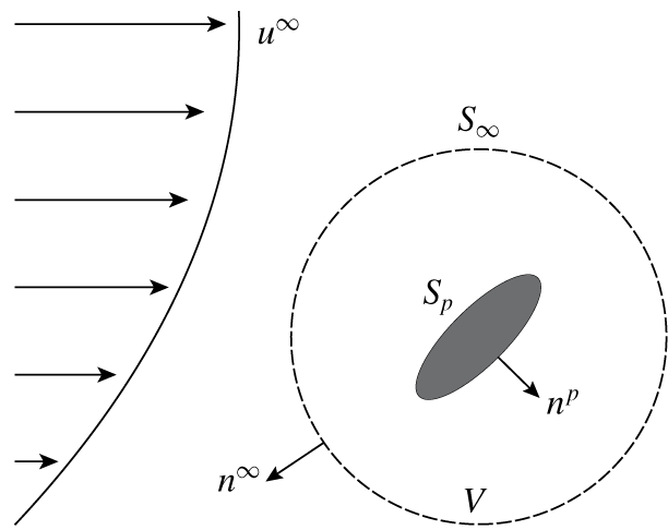
Schematics of the system set-up.

2.2 Integral expressions for polymeric force/torque on particle
To evaluate the polymeric force  $F_{i}^{p}$ and torque
 $T_{i}^{p}$ on the particle (i.e. the force/torque in excess of the Newtonian contribution), we first construct a control volume
 $V$ containing the particle with its surface denoted as
 $S_{\infty }$. We also define the particle surface to be
 $S_{p}$. The outward normals on
 $S_{\infty }$ and
 $S_{p}$ are denoted as
 $n_{i}^{\infty }$ and
 $n_{i}^{p}$, respectively. Figure 1 shows the system set-up.
From (2.4) we know that
 $$\begin{eqnarray}\int _{V}\frac{\unicode[STIX]{x2202}\unicode[STIX]{x1D61B}_{ij}}{\unicode[STIX]{x2202}x_{j}}\,\text{d}V=0.\end{eqnarray}$$
By the divergence theorem, we get
 $$\begin{eqnarray}\int _{S_{\infty }}\unicode[STIX]{x1D61B}_{ij}n_{j}^{\infty }\,\text{d}S=\int _{S_{p}}\unicode[STIX]{x1D61B}_{ij}n_{j}^{p}\,\text{d}S.\end{eqnarray}$$
Equation (2.14) indicates that the force on the particle can be evaluated over any closed surface  $S_{\infty }$ as long as it completely contains the particle. This statement is true for torque as well. Next, we extract the polymeric contribution to the total stress tensor
 $\unicode[STIX]{x1D61B}_{ij}$ and perform integration over a spherical surface
 $S_{\infty }$ containing the particle:
 $$\begin{eqnarray}\displaystyle \frac{2}{\unicode[STIX]{x1D713}_{1}}F_{i}^{p} & = & \displaystyle \int _{S_{\infty }}\left(\frac{1}{\unicode[STIX]{x1D707}}\frac{\unicode[STIX]{x2202}P^{N}}{\unicode[STIX]{x2202}t}\unicode[STIX]{x1D6FF}_{ij}-\frac{\unicode[STIX]{x2202}\dot{\unicode[STIX]{x1D6FE}}_{ij}}{\unicode[STIX]{x2202}t}\right)n_{j}^{\infty }\,\text{d}S+\int _{S_{\infty }}\left(\frac{1}{\unicode[STIX]{x1D707}}u_{m}\frac{\unicode[STIX]{x2202}P^{N}}{\unicode[STIX]{x2202}x_{m}}\unicode[STIX]{x1D6FF}_{ij}-u_{m}\frac{\unicode[STIX]{x2202}\dot{\unicode[STIX]{x1D6FE}}_{ij}}{\unicode[STIX]{x2202}x_{m}}\right)n_{j}^{\infty }\,\text{d}S\nonumber\\ \displaystyle & & \displaystyle +\,\int _{S_{\infty }}\left(\frac{1}{4}\dot{\unicode[STIX]{x1D6FE}}_{km}\dot{\unicode[STIX]{x1D6FE}}_{mk}\unicode[STIX]{x1D6FF}_{ij}-\frac{\unicode[STIX]{x2202}u_{k}}{\unicode[STIX]{x2202}x_{i}}\frac{\unicode[STIX]{x2202}u_{k}}{\unicode[STIX]{x2202}x_{j}}+\frac{\unicode[STIX]{x2202}u_{i}}{\unicode[STIX]{x2202}x_{k}}\frac{\unicode[STIX]{x2202}u_{j}}{\unicode[STIX]{x2202}x_{k}}\right)n_{j}^{\infty }\,\text{d}S,\end{eqnarray}$$
 $$\begin{eqnarray}\displaystyle \frac{2}{\unicode[STIX]{x1D713}_{1}}T_{i}^{p} & = & \displaystyle \int _{S_{\infty }}\unicode[STIX]{x1D700}_{ijk}x_{j}\left(\frac{1}{\unicode[STIX]{x1D707}}\frac{\unicode[STIX]{x2202}P^{N}}{\unicode[STIX]{x2202}t}\unicode[STIX]{x1D6FF}_{kp}-\frac{\dot{\unicode[STIX]{x2202}\unicode[STIX]{x1D6FE}}_{kp}}{\unicode[STIX]{x2202}t}\right)n_{p}^{\infty }\,\text{d}S\nonumber\\ \displaystyle & & \displaystyle +\,\int _{S_{\infty }}\unicode[STIX]{x1D700}_{ijk}x_{j}\left(\frac{1}{\unicode[STIX]{x1D707}}u_{m}\frac{\unicode[STIX]{x2202}P^{N}}{\unicode[STIX]{x2202}x_{m}}\unicode[STIX]{x1D6FF}_{kp}-u_{m}\frac{\unicode[STIX]{x2202}\dot{\unicode[STIX]{x1D6FE}}_{kp}}{\unicode[STIX]{x2202}x_{m}}\right)n_{p}^{\infty }\,\text{d}S\nonumber\\ \displaystyle & & \displaystyle +\,\int _{S_{\infty }}\unicode[STIX]{x1D700}_{ijk}x_{j}\left(\frac{1}{4}\dot{\unicode[STIX]{x1D6FE}}_{nm}\dot{\unicode[STIX]{x1D6FE}}_{mn}\unicode[STIX]{x1D6FF}_{kp}-\frac{\unicode[STIX]{x2202}u_{m}}{\unicode[STIX]{x2202}x_{k}}\frac{\unicode[STIX]{x2202}u_{m}}{\unicode[STIX]{x2202}x_{p}}+\frac{\unicode[STIX]{x2202}u_{k}}{\unicode[STIX]{x2202}x_{m}}\frac{\unicode[STIX]{x2202}u_{p}}{\unicode[STIX]{x2202}x_{m}}\right)n_{p}^{\infty }\,\text{d}S.\end{eqnarray}$$
By employing the divergence theorem, the polymeric force and torque expressions can be modified to
 $$\begin{eqnarray}\displaystyle \frac{2}{\unicode[STIX]{x1D713}_{1}}F_{i}^{p} & = & \displaystyle \int _{S_{\infty }}\left(\frac{1}{\unicode[STIX]{x1D707}}\frac{\unicode[STIX]{x2202}P^{N}}{\unicode[STIX]{x2202}t}\unicode[STIX]{x1D6FF}_{ij}-\frac{\unicode[STIX]{x2202}\dot{\unicode[STIX]{x1D6FE}}_{ij}}{\unicode[STIX]{x2202}t}\right)n_{j}^{\infty }\,\text{d}S\int _{S_{\infty }}\frac{1}{\unicode[STIX]{x1D707}}\frac{\unicode[STIX]{x2202}u_{m}}{\unicode[STIX]{x2202}x_{j}}(P^{N}\unicode[STIX]{x1D6FF}_{ij}-\unicode[STIX]{x1D707}\dot{\unicode[STIX]{x1D6FE}}_{ij})n_{m}^{\infty }\,\text{d}S\nonumber\\ \displaystyle & & \displaystyle +\,\int _{S_{\infty }}\left(\frac{1}{4}\dot{\unicode[STIX]{x1D6FE}}_{km}\dot{\unicode[STIX]{x1D6FE}}_{mk}\unicode[STIX]{x1D6FF}_{ij}-\frac{\unicode[STIX]{x2202}u_{k}}{\unicode[STIX]{x2202}x_{i}}\frac{\unicode[STIX]{x2202}u_{k}}{\unicode[STIX]{x2202}x_{j}}+\frac{\unicode[STIX]{x2202}u_{i}}{\unicode[STIX]{x2202}x_{k}}\frac{\unicode[STIX]{x2202}u_{j}}{\unicode[STIX]{x2202}x_{k}}\right)n_{j}^{\infty }\,\text{d}S,\end{eqnarray}$$
 $$\begin{eqnarray}\displaystyle \frac{2}{\unicode[STIX]{x1D713}_{1}}T_{i}^{p} & = & \displaystyle \int _{S_{\infty }}\unicode[STIX]{x1D700}_{ijk}x_{j}\left(\frac{1}{\unicode[STIX]{x1D707}}\frac{\unicode[STIX]{x2202}P^{N}}{\unicode[STIX]{x2202}t}\unicode[STIX]{x1D6FF}_{kp}-\frac{\unicode[STIX]{x2202}\dot{\unicode[STIX]{x1D6FE}}_{kp}}{\unicode[STIX]{x2202}t}\right)n_{p}^{\infty }\,\text{d}S\int _{S_{\infty }}\unicode[STIX]{x1D700}_{ijk}x_{j}\frac{\unicode[STIX]{x2202}u_{m}}{\unicode[STIX]{x2202}x_{p}}\left(\frac{1}{\unicode[STIX]{x1D707}}P^{N}\unicode[STIX]{x1D6FF}_{kp}-\dot{\unicode[STIX]{x1D6FE}}_{kp}\right)n_{m}^{\infty }\,\text{d}S\nonumber\\ \displaystyle & & \displaystyle -\,\int _{S_{\infty }}\unicode[STIX]{x1D700}_{imk}\left(\frac{1}{\unicode[STIX]{x1D707}}P^{N}\unicode[STIX]{x1D6FF}_{kp}-\dot{\unicode[STIX]{x1D6FE}}_{kp}\right)u_{m}n_{p}^{\infty }\,\text{d}S\nonumber\\ \displaystyle & & \displaystyle +\,\int _{S_{\infty }}\unicode[STIX]{x1D700}_{ijk}x_{j}\left(\frac{1}{4}\dot{\unicode[STIX]{x1D6FE}}_{nm}\dot{\unicode[STIX]{x1D6FE}}_{mn}\unicode[STIX]{x1D6FF}_{kp}-\frac{\unicode[STIX]{x2202}u_{m}}{\unicode[STIX]{x2202}x_{k}}\frac{\unicode[STIX]{x2202}u_{m}}{\unicode[STIX]{x2202}x_{p}}+\frac{\unicode[STIX]{x2202}u_{k}}{\unicode[STIX]{x2202}x_{m}}\frac{\unicode[STIX]{x2202}u_{p}}{\unicode[STIX]{x2202}x_{m}}\right)n_{p}^{\infty }\,\text{d}S.\end{eqnarray}$$
Equations (2.17) and (2.18) allow us to solve for the polymeric force and torque once we acquire information on the velocity field  $u_{i}$ and pressure field
 $P^{N}$, which are the velocity and pressure fields for the Stokes flow past the particle in the same geometry. In § 2.3 we employ a multipole expansion to obtain these fields and hence simplify the analytical expressions for the polymeric force and torque.
2.3 Multipole expansion and symmetry analysis – analytical solution to resistance functions for arbitrarily shaped particles
For a Newtonian fluid in the creeping flow regime, the fluid disturbance velocity and pressure fields far away from the particle surface can be expressed using a multipole expansion (Kim & Karrila Reference Kim and Karrila2013) as
 $$\begin{eqnarray}\displaystyle & \displaystyle u_{i}-u_{i}^{\infty }=-\frac{1}{8\unicode[STIX]{x03C0}\unicode[STIX]{x1D707}}F_{j}^{(1)}\unicode[STIX]{x1D60E}_{ij}+\frac{1}{8\unicode[STIX]{x03C0}\unicode[STIX]{x1D707}}\unicode[STIX]{x1D60D}_{jk}^{(2)}\frac{\unicode[STIX]{x2202}\unicode[STIX]{x1D60E}_{ij}}{\unicode[STIX]{x2202}x_{k}}-\frac{1}{16\unicode[STIX]{x03C0}\unicode[STIX]{x1D707}}\unicode[STIX]{x1D60D}_{jkm}^{(3)}\frac{\unicode[STIX]{x2202}\unicode[STIX]{x1D60E}_{ij}}{\unicode[STIX]{x2202}x_{k}\unicode[STIX]{x2202}x_{m}}+\cdots \,, & \displaystyle\end{eqnarray}$$
 $$\begin{eqnarray}\displaystyle & \displaystyle P^{N}-P^{N\infty }=-\frac{1}{8\unicode[STIX]{x03C0}}F_{j}^{(1)}\unicode[STIX]{x1D70B}_{j}+\frac{1}{8\unicode[STIX]{x03C0}}\unicode[STIX]{x1D60D}_{jk}^{(2)}\frac{\unicode[STIX]{x2202}\unicode[STIX]{x1D70B}_{j}}{\unicode[STIX]{x2202}x_{k}}-\frac{1}{16\unicode[STIX]{x03C0}}\unicode[STIX]{x1D60D}_{jkm}^{(3)}\frac{\unicode[STIX]{x2202}\unicode[STIX]{x1D70B}_{j}}{\unicode[STIX]{x2202}x_{k}\unicode[STIX]{x2202}x_{m}}+\cdots \,, & \displaystyle\end{eqnarray}$$
where  $\unicode[STIX]{x1D60E}_{ij}$ and
 $\unicode[STIX]{x1D70B}_{i}$ are the Green’s functions for velocity and pressure, respectively. The expressions
 $\unicode[STIX]{x1D60D}_{k_{1}\ldots k_{n}}^{(n)}$ are the force moments (i.e. monopole, dipole, etc.) on the particle in Stokes flow. Thus
 $$\begin{eqnarray}\displaystyle \left.\begin{array}{@{}l@{}}\unicode[STIX]{x1D60E}_{ij}={\displaystyle \frac{\unicode[STIX]{x1D6FF}_{ij}}{r}}+{\displaystyle \frac{x_{i}x_{j}}{r^{3}}},\quad \unicode[STIX]{x1D70B}_{i}={\displaystyle \frac{2x_{i}}{r^{3}}},\quad r=(x_{i}x_{i})^{1/2},\\[10.0pt] \unicode[STIX]{x1D60D}_{k_{1}\ldots k_{n}}^{(n)}=\displaystyle \int _{S_{p}}(\unicode[STIX]{x1D70E}_{k_{1}m}^{N}n_{m}^{p})x_{k_{2}}\cdots x_{k_{n}}\,\text{d}S,\\[15.0pt] \unicode[STIX]{x1D70E}_{ij}^{N}=-P^{N}\unicode[STIX]{x1D6FF}_{ij}+\unicode[STIX]{x1D707}\dot{\unicode[STIX]{x1D6FE}}_{ij},\\[5.0pt] -{\displaystyle \frac{\unicode[STIX]{x2202}P^{N\infty }}{\unicode[STIX]{x2202}x_{i}}}+\unicode[STIX]{x1D707}{\displaystyle \frac{\unicode[STIX]{x2202}^{2}u_{i}^{\infty }}{\unicode[STIX]{x2202}x_{j}\unicode[STIX]{x2202}x_{j}}}=0.\end{array}\right\} & & \displaystyle\end{eqnarray}$$
Equations (2.19) and (2.20) hold for any particle shape as long as the position is far away from the particle surface.
We will evaluate an analytical expression for the polymer force and torque in (2.17) and (2.18) by substituting the far-field velocity and pressure fields in (2.19) and (2.20). To simplify the mathematics, we note that only a small number of terms will contribute to the integrals. Since the integrals are evaluated on a spherical surface far away from the particle (i.e.  $r\rightarrow \infty$), one should expect only the terms of
 $O(r^{-2})$ in the integrand of (2.17) and (2.18) to contribute to the polymeric force and torque since the surface element
 $\text{d}S$ is proportional to
 $r^{2}$.
For the integrals in (2.17), we find that the following vector and tensor combinations will contribute to the polymeric force:
 $$\begin{eqnarray}\frac{\unicode[STIX]{x2202}F_{i}^{(1)}}{\unicode[STIX]{x2202}t},\quad \unicode[STIX]{x1D6E4}_{ij}^{(2)}F_{k}^{(1)},\quad \unicode[STIX]{x1D6E4}_{ijk}^{(3)}\unicode[STIX]{x1D60D}_{mp}^{(2)}.\end{eqnarray}$$
Following the same ideas, we expect the terms of  $O(r^{-2})$ in the integrand of (2.18) will contribute to the polymeric torque:
 $$\begin{eqnarray}\frac{\unicode[STIX]{x2202}T_{i}^{N}}{\unicode[STIX]{x2202}t},\quad \unicode[STIX]{x1D60D}_{imk}^{(3)}\unicode[STIX]{x1D6E4}_{pqj}^{(3)},\quad \unicode[STIX]{x1D60D}_{ik}^{(2)}\unicode[STIX]{x1D6E4}_{mj}^{(2)},\quad u_{i}^{c}F_{j}^{(1)}.\end{eqnarray}$$
Next we perform tensor decomposition of the force moments  $\unicode[STIX]{x1D60D}_{ij}^{(2)}$,
 $\unicode[STIX]{x1D60D}_{ijk}^{(3)}$ and external velocity gradients
 $\unicode[STIX]{x1D6E4}_{ij}^{(2)}$,
 $\unicode[STIX]{x1D6E4}_{ijk}^{(3)}$ into irreducible forms:
 $$\begin{eqnarray}\displaystyle & \displaystyle \unicode[STIX]{x1D6E4}_{ij}^{(2)}=\unicode[STIX]{x1D60C}_{ij}-\unicode[STIX]{x1D700}_{ijk}\unicode[STIX]{x1D6FA}_{k}, & \displaystyle\end{eqnarray}$$
 $$\begin{eqnarray}\displaystyle & \displaystyle \unicode[STIX]{x1D60D}_{ij}^{(2)}=\unicode[STIX]{x1D61A}_{ij}-{\textstyle \frac{1}{2}}\unicode[STIX]{x1D700}_{ijk}T_{k}^{N}, & \displaystyle\end{eqnarray}$$
 $$\begin{eqnarray}\displaystyle & \displaystyle \unicode[STIX]{x1D6E4}_{ijk}^{(3)}=\unicode[STIX]{x1D6E4}_{ijk}^{(3)^{\prime }}-{\textstyle \frac{1}{6}}\unicode[STIX]{x1D6FA}_{im}\unicode[STIX]{x1D700}_{mjk}-{\textstyle \frac{1}{3}}\unicode[STIX]{x1D6FA}_{km}\unicode[STIX]{x1D700}_{mij}+{\textstyle \frac{1}{10}}(-\unicode[STIX]{x1D70F}_{k}\unicode[STIX]{x1D6FF}_{ij}-\unicode[STIX]{x1D70F}_{j}\unicode[STIX]{x1D6FF}_{ik}+4\unicode[STIX]{x1D70F}_{i}\unicode[STIX]{x1D6FF}_{kj}), & \displaystyle\end{eqnarray}$$
 $$\begin{eqnarray}\displaystyle \unicode[STIX]{x1D60D}_{ijk}^{(3)} & = & \displaystyle \unicode[STIX]{x1D60D}_{ijk}^{(3)^{\prime }}-{\textstyle \frac{1}{6}}\unicode[STIX]{x1D6E9}_{im}\unicode[STIX]{x1D700}_{mjk}-{\textstyle \frac{1}{3}}\unicode[STIX]{x1D6E9}_{km}\unicode[STIX]{x1D700}_{mij}+{\textstyle \frac{1}{10}}(-H_{k}\unicode[STIX]{x1D6FF}_{ij}-H_{j}\unicode[STIX]{x1D6FF}_{ik}+4H_{i}\unicode[STIX]{x1D6FF}_{kj})\nonumber\\ \displaystyle & & \displaystyle +\,{\textstyle \frac{1}{10}}(3B_{k}\unicode[STIX]{x1D6FF}_{ij}+3B_{j}\unicode[STIX]{x1D6FF}_{ik}-2B_{i}\unicode[STIX]{x1D6FF}_{kj}).\end{eqnarray}$$
The right-hand sides of (2.22)–(2.25) are the irreducible elements of the force moments and the external velocity gradients. For example,  $\unicode[STIX]{x1D60C}_{ij}$ and
 $\unicode[STIX]{x1D6FA}_{i}$ are the rate of strain and angular velocity of the external flow, while
 $\unicode[STIX]{x1D61A}_{ij}$ and
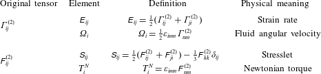
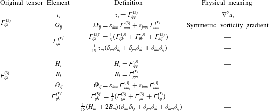
 $\unicode[STIX]{x1D61B}_{i}^{N}$ are the stresslet and torque in a Newtonian fluid. The definitions of each of the irreducible elements are detailed in tables 1 and 2.
Based on the decomposition, the following combinations of the irreducible tensors can possibly contribute to the polymeric force:
 $$\begin{eqnarray}\displaystyle \frac{\unicode[STIX]{x2202}F_{i}^{(1)}}{\unicode[STIX]{x2202}t},\quad \unicode[STIX]{x1D60C}_{ij}F_{j}^{(1)},\quad \unicode[STIX]{x1D700}_{ijk}F_{j}^{(1)}\unicode[STIX]{x1D6FA}_{k},\quad \unicode[STIX]{x1D6E4}_{ijk}^{(3)^{\prime }}\unicode[STIX]{x1D61A}_{jk},\quad \unicode[STIX]{x1D61A}_{ij}\unicode[STIX]{x1D70F}_{j},\quad \unicode[STIX]{x1D700}_{ijk}\unicode[STIX]{x1D6FA}_{jm}\unicode[STIX]{x1D61A}_{mk},\quad \unicode[STIX]{x1D700}_{ijk}T_{j}^{N}\unicode[STIX]{x1D70F}_{k},\quad \unicode[STIX]{x1D6FA}_{ij}T_{j}^{N}. & & \displaystyle \nonumber\end{eqnarray}$$
Similarly, the following combinations can possibly contribute to the polymeric torque:
 $$\begin{eqnarray}\displaystyle \frac{\unicode[STIX]{x2202}T_{i}^{N}}{\unicode[STIX]{x2202}t},\quad \unicode[STIX]{x1D700}_{ijk}u_{j}^{c}F_{k}^{(1)},\quad \unicode[STIX]{x1D700}_{ijk}\unicode[STIX]{x1D60C}_{jm}\unicode[STIX]{x1D61A}_{mk},\quad \unicode[STIX]{x1D60C}_{ij}T_{j}^{N},\quad \unicode[STIX]{x1D61A}_{ij}\unicode[STIX]{x1D6FA}_{j},\quad \unicode[STIX]{x1D700}_{ijk}T_{j}^{N}\unicode[STIX]{x1D6FA}_{k},\quad \unicode[STIX]{x1D700}_{ijk}\unicode[STIX]{x1D6E4}_{jpq}^{(3)^{\prime }}\unicode[STIX]{x1D60D}_{kpq}^{(3)^{\prime }}, & & \displaystyle \nonumber\\ \displaystyle \unicode[STIX]{x1D6E4}_{ijk}^{(3)^{\prime }}\unicode[STIX]{x1D6E9}_{jk},\quad \unicode[STIX]{x1D700}_{ijk}\unicode[STIX]{x1D70F}_{j}H_{k},\quad \unicode[STIX]{x1D700}_{ijk}\unicode[STIX]{x1D70F}_{j}B_{k},\quad \unicode[STIX]{x1D6E9}_{ij}\unicode[STIX]{x1D70F}_{j},\quad \unicode[STIX]{x1D60D}_{ijk}^{(3)^{\prime }}\unicode[STIX]{x1D6FA}_{jk},\quad \unicode[STIX]{x1D6FA}_{ij}H_{j},\quad \unicode[STIX]{x1D6FA}_{ij}B_{j},\quad \unicode[STIX]{x1D700}_{ijk}\unicode[STIX]{x1D6FA}_{jm}\unicode[STIX]{x1D6E9}_{mk}. & & \displaystyle \nonumber\end{eqnarray}$$
Decomposition elements for the second-order tensors  $\unicode[STIX]{x1D60D}_{ij}^{(2)}$ and
 $\unicode[STIX]{x1D6E4}_{ij}^{(2)}$.

Decomposition elements for the third-order tensors  $\unicode[STIX]{x1D60D}_{ijk}^{(3)}$ and
 $\unicode[STIX]{x1D6E4}_{ijk}^{(3)}$.

The polymeric force and torque will be a linear combination of the terms listed above. To determine the coefficients for each possible combination, for instance  $\unicode[STIX]{x1D60C}_{ij}F_{j}^{(1)}$, we choose the force moments and external velocity gradients such that the only contribution to the polymeric force and torque will come from
 $\unicode[STIX]{x1D60C}_{ij}F_{j}^{(1)}$, and then directly integrate (2.17) and (2.18). Repeating this procedure for all possible tensor combinations, we have the following expressions for the polymeric force and torque:
 $$\begin{eqnarray}\displaystyle \frac{2\unicode[STIX]{x1D707}}{\unicode[STIX]{x1D713}_{1}}F_{i}^{p} & = & \displaystyle -\frac{\unicode[STIX]{x2202}F_{i}^{(1)}}{\unicode[STIX]{x2202}t}-\unicode[STIX]{x1D60C}_{ij}F_{j}^{(1)}-\unicode[STIX]{x1D700}_{ijk}F_{j}^{(1)}\unicode[STIX]{x1D6FA}_{k}-\unicode[STIX]{x1D6E4}_{ijk}^{(3)^{\prime }}\unicode[STIX]{x1D61A}_{jk}-{\textstyle \frac{3}{10}}\unicode[STIX]{x1D61A}_{ij}\unicode[STIX]{x1D70F}_{j}\nonumber\\ \displaystyle & & \displaystyle +\,{\textstyle \frac{1}{6}}\unicode[STIX]{x1D700}_{ijk}\unicode[STIX]{x1D6FA}_{jm}\unicode[STIX]{x1D61A}_{mk}+{\textstyle \frac{1}{4}}\unicode[STIX]{x1D700}_{ijk}T_{j}^{N}\unicode[STIX]{x1D70F}_{k}-{\textstyle \frac{1}{4}}\unicode[STIX]{x1D6FA}_{ij}T_{j}^{N},\end{eqnarray}$$
 $$\begin{eqnarray}\displaystyle \frac{2\unicode[STIX]{x1D707}}{\unicode[STIX]{x1D713}_{1}}T_{i}^{p} & = & \displaystyle -\frac{\unicode[STIX]{x2202}T_{i}^{N}}{\unicode[STIX]{x2202}t}+\unicode[STIX]{x1D700}_{ijk}u_{j}^{c}F_{k}^{(1)}+2\unicode[STIX]{x1D700}_{ijk}\unicode[STIX]{x1D60C}_{jm}\unicode[STIX]{x1D61A}_{mk}-\unicode[STIX]{x1D700}_{ijk}T_{j}^{N}\unicode[STIX]{x1D6FA}_{k}+{\textstyle \frac{3}{2}}\unicode[STIX]{x1D700}_{ijk}\unicode[STIX]{x1D6E4}_{jpq}^{(3)^{\prime }}\unicode[STIX]{x1D60D}_{kpq}^{(3)^{\prime }}\nonumber\\ \displaystyle & & \displaystyle +\,{\textstyle \frac{1}{5}}\unicode[STIX]{x1D700}_{ijk}\unicode[STIX]{x1D70F}_{j}H_{k}-{\textstyle \frac{1}{10}}\unicode[STIX]{x1D700}_{ijk}\unicode[STIX]{x1D70F}_{j}B_{k}+{\textstyle \frac{1}{6}}\unicode[STIX]{x1D700}_{ijk}\unicode[STIX]{x1D6FA}_{jm}\unicode[STIX]{x1D6E9}_{mk}.\end{eqnarray}$$
This is one of the main results of this paper. The effect of particle shape comes through the force moments ( $F_{i}^{(1)}$,
 $\unicode[STIX]{x1D61A}_{ij}$,
 $T_{i}^{N}$, …) on the particle in Stokes flow, which are related to the external flow fields (
 $u_{i}^{c}$,
 $\unicode[STIX]{x1D60C}_{ij}$,
 $\unicode[STIX]{x1D6FA}_{i}$, …) through a resistance matrix. For example, if we are examining a sphere of radius
 $R$ in an external flow, the force moments come from the Stokes drag/torque/stresslet formulae:
 $F_{i}^{(1)}=6\unicode[STIX]{x03C0}\unicode[STIX]{x1D707}R(u_{i}^{c}-U_{i})$,
 $\unicode[STIX]{x1D61B}_{i}^{N}=8\unicode[STIX]{x03C0}\unicode[STIX]{x1D707}R^{3}(\unicode[STIX]{x1D6FA}_{i}-\unicode[STIX]{x1D714}_{i})$,
 $\unicode[STIX]{x1D61A}_{ij}=(20\unicode[STIX]{x03C0}/3)\unicode[STIX]{x1D707}R^{3}\unicode[STIX]{x1D60C}_{ij}$, etc., where
 $U_{i}$ and
 $\unicode[STIX]{x1D714}_{i}$ are the translational and rotational velocities of the particle. If we are examining a slender body of length
 $L$, aspect ratio
 $A_{R}$ and orientation vector
 $p_{i}$, the force moments come from slender-body theory:
 $F_{i}^{(1)}=(4\unicode[STIX]{x03C0}\unicode[STIX]{x1D707}L/\ln (2A_{R}))(\unicode[STIX]{x1D6FF}_{ij}-{\textstyle \frac{1}{2}}p_{i}p_{j})(u_{j}^{c}-U_{j})$,
 $\unicode[STIX]{x1D61B}_{i}^{N}=(\unicode[STIX]{x03C0}\unicode[STIX]{x1D707}L^{3}/(3\ln (2A_{R})))[(\unicode[STIX]{x1D6FF}_{ij}-p_{i}p_{j})(\unicode[STIX]{x1D6FA}_{j}-\unicode[STIX]{x1D714}_{j})-\unicode[STIX]{x1D716}_{ijk}p_{j}E_{km}p_{m}]$, etc. The main point to take away from this section is that, if one knows the force/torque/stresslet, etc. on an arbitrarily shaped particle in a Newtonian fluid, one can determine the polymeric force and torque on the same particle using formulae (2.26) and (2.27). We note that the methodologies applied in this and the following section are only valid when we impose the assumption
 $\unicode[STIX]{x1D713}_{1}=-2\unicode[STIX]{x1D713}_{2}$, under which the flow dynamics can be analysed using the linear superposition techniques developed from the Stokes flows. The analysis techniques are not valid for the general case
 $\unicode[STIX]{x1D713}_{1}\neq -2\unicode[STIX]{x1D713}_{2}$, where the flow dynamics are nonlinear. We further note that the time-dependent terms
 $\unicode[STIX]{x2202}F_{i}^{(1)}/\unicode[STIX]{x2202}t$ and
 $\unicode[STIX]{x2202}T_{i}^{N}/\unicode[STIX]{x2202}t$ in (2.26) and (2.27) will be negligible for a force/torque-free particle. In § 2.4 we perform a perturbation expansion analysis to clarify this idea.
2.4 Perturbation expansion analysis
For a system as defined in § 2.1, when force/torque-free, the total force and torque on the particle are identically zero:
 $$\begin{eqnarray}F_{i}^{(1)}+F_{i}^{p}=0,\quad T_{i}^{N}+T_{i}^{p}=0.\end{eqnarray}$$
We perform a perturbation expansion on the particle’s translational and rotational velocities ( $U_{i},\unicode[STIX]{x1D714}_{i}$) using the small parameter
 $Wi$:
 $$\begin{eqnarray}\left.\begin{array}{@{}l@{}}U_{i}=U_{i}^{[0]}+Wi\,U_{i}^{[1]}+\cdots \,,\\[3.0pt] \unicode[STIX]{x1D714}_{i}=\unicode[STIX]{x1D714}_{i}^{[0]}+Wi\,\unicode[STIX]{x1D714}_{i}^{[1]}+\cdots \,,\end{array}\right\}\quad Wi\ll 1,\end{eqnarray}$$
where  $U_{i}^{[n]}$ and
 $\unicode[STIX]{x1D714}_{i}^{[n]}$ represent the particle’s translational and rotational velocities at
 $O(Wi^{n})$. Our goal is to obtain the
 $O(Wi)$ correction to the particle motion.
If we scale all velocities by a characteristic scale  $u^{m}$, all lengths by a characteristic length
 $L$, times and rotational velocities by
 $L/u^{m}$, forces by
 $\unicode[STIX]{x1D707}u^{m}L$ and torques by
 $\unicode[STIX]{x1D707}u^{m}L^{2}$, the force/torque-free requirement indicates that the Newtonian force and torque at leading order are identically zero:
 $$\begin{eqnarray}F_{i}^{(1),[0]}=0,\quad T_{i}^{N,[0]}=0.\end{eqnarray}$$
At  $O(Wi)$, the Newtonian force/torque evaluated using
 $U_{i}^{[1]}$ and
 $\unicode[STIX]{x1D714}_{i}^{[1]}$ are in balance with the polymeric force/torque evaluated using
 $U_{i}^{[0]}$ and
 $\unicode[STIX]{x1D714}_{i}^{[0]}$:
 $$\begin{eqnarray}\left.\begin{array}{@{}l@{}}F_{i}^{(1),[1]}+F_{i}^{p,[0]}=0,\\[3.0pt] T_{i}^{N,[1]}+T_{i}^{p,[0]}=0.\end{array}\right\}\end{eqnarray}$$
Owing to the Newtonian force/torque vanishing at  $O(1)$, the time-dependent terms
 $\unicode[STIX]{x2202}F_{i}^{(1),[0]}/\unicode[STIX]{x2202}t$ and
 $\unicode[STIX]{x2202}T_{i}^{N,[0]}/\unicode[STIX]{x2202}t$ will vanish in the polymeric force and torque expression in (2.31). Thus, for a viscoelastic fluid in the limit of small Weissenberg number (
 $Wi\ll 1$) and co-rotational limit (
 $\unicode[STIX]{x1D713}_{1}=-2\unicode[STIX]{x1D713}_{2}$), the polymer stresses and pressures will be unsteady, but the unsteady effects will cancel out when computing the polymer force and torque to
 $O(Wi)$. This argument is consistent with Brunn (Reference Brunn1977), where he also investigated the dynamics of a rigid particle under these same assumptions and found that the force and torque appear steady at
 $O(Wi)$.
In § 2.5, we will introduce the resistance matrix of a general ellipsoid in Stokes flow, and use (2.26) and (2.27) to calculate its motion in a second-order fluid when  $\unicode[STIX]{x1D713}_{1}=-2\unicode[STIX]{x1D713}_{2}$ under a general quadratic flow field. We will use boundary element simulations in § 2.6 to verify the results shown here.
2.5 Resistance matrix for a general ellipsoid in Stokes flow
We extend the original resistance relationship in Kim & Karrila (Reference Kim and Karrila2013) to consider the motion of an arbitrarily shaped particle in a quadratic flow:
 $$\begin{eqnarray}\displaystyle \left(\begin{array}{@{}c@{}}\boldsymbol{F}^{(1)}\\ \boldsymbol{T}^{N}\\ \unicode[STIX]{x1D64E}\\ \unicode[STIX]{x1D641}^{(3)}\end{array}\right)=\unicode[STIX]{x1D707}\left(\begin{array}{@{}cccc@{}}\unicode[STIX]{x1D63C} & \widetilde{\unicode[STIX]{x1D63D}} & \widetilde{\unicode[STIX]{x1D642}} & \widetilde{\unicode[STIX]{x1D64A}}\\ \unicode[STIX]{x1D63D} & \unicode[STIX]{x1D63E} & \widetilde{\unicode[STIX]{x1D648}} & \widetilde{\unicode[STIX]{x1D64C}}\\ \unicode[STIX]{x1D642} & \unicode[STIX]{x1D648} & \unicode[STIX]{x1D649} & \widetilde{\unicode[STIX]{x1D64D}}\\ \unicode[STIX]{x1D64A} & \unicode[STIX]{x1D64C} & \unicode[STIX]{x1D64D} & \unicode[STIX]{x1D651}\end{array}\right)\left(\begin{array}{@{}c@{}}\boldsymbol{u}^{c}-\boldsymbol{U}\\ \unicode[STIX]{x1D734}-\unicode[STIX]{x1D74E}\\ \unicode[STIX]{x1D640}\\ \unicode[STIX]{x1D71E}^{(3)}\end{array}\right), & & \displaystyle \nonumber\end{eqnarray}$$
where  $\boldsymbol{U}$ and
 $\unicode[STIX]{x1D74E}$ denote the translation and rotation of the particle, respectively. Specifically, the resistance matrix can be written in index notation:
 $$\begin{eqnarray}\displaystyle \left.\begin{array}{@{}l@{}}F_{i}^{(1)}=\unicode[STIX]{x1D707}\unicode[STIX]{x1D608}_{ij}(u_{j}^{c}-U_{j})+\unicode[STIX]{x1D707}\widetilde{B}_{ij}(\unicode[STIX]{x1D6FA}_{j}-\unicode[STIX]{x1D714}_{j})+\unicode[STIX]{x1D707}\widetilde{G}_{ijk}\unicode[STIX]{x1D60C}_{jk}+\unicode[STIX]{x1D707}\widetilde{O}_{ijkl}\unicode[STIX]{x1D6E4}_{jkl}^{(3)},\\[3.0pt] T_{i}^{N}=\unicode[STIX]{x1D707}\unicode[STIX]{x1D609}_{ij}(u_{j}^{c}-U_{j})+\unicode[STIX]{x1D707}\unicode[STIX]{x1D60A}_{ij}(\unicode[STIX]{x1D6FA}_{j}-\unicode[STIX]{x1D714}_{j})+\unicode[STIX]{x1D707}\widetilde{M}_{ijk}\unicode[STIX]{x1D60C}_{jk}+\unicode[STIX]{x1D707}\widetilde{Q}_{ijkl}\unicode[STIX]{x1D6E4}_{jkl}^{(3)},\\ \unicode[STIX]{x1D61A}_{ij}=\unicode[STIX]{x1D707}\unicode[STIX]{x1D60E}_{ijk}(u_{k}^{c}-U_{k})+\unicode[STIX]{x1D707}\unicode[STIX]{x1D614}_{ijk}(\unicode[STIX]{x1D6FA}_{k}-\unicode[STIX]{x1D714}_{k})+\unicode[STIX]{x1D707}\unicode[STIX]{x1D615}_{ijkl}\unicode[STIX]{x1D60C}_{kl}+\unicode[STIX]{x1D707}\widetilde{R}_{ijklw}\unicode[STIX]{x1D6E4}_{klw}^{(3)},\\[3.0pt] \unicode[STIX]{x1D60D}_{ijk}^{(3)}=\unicode[STIX]{x1D707}\unicode[STIX]{x1D616}_{ijkl}(u_{l}^{c}-U_{l})+\unicode[STIX]{x1D707}\unicode[STIX]{x1D618}_{ijkl}(\unicode[STIX]{x1D6FA}_{l}-\unicode[STIX]{x1D714}_{l})+\unicode[STIX]{x1D707}\unicode[STIX]{x1D619}_{ijklw}\unicode[STIX]{x1D60C}_{lw}+\unicode[STIX]{x1D707}\unicode[STIX]{x1D61D}_{ijklwx}\unicode[STIX]{x1D6E4}_{lwx}^{(3)}.\end{array}\right\} & & \displaystyle\end{eqnarray}$$
For a general triaxial ellipsoid, one obtains
 $$\begin{eqnarray}\displaystyle \left.\begin{array}{@{}l@{}}\widetilde{B}_{ij}=\unicode[STIX]{x1D609}_{ij}=0,\quad \widetilde{G}_{ijk}=\unicode[STIX]{x1D60E}_{ijk}=0,\\ \widetilde{Q}_{ijkl}=\unicode[STIX]{x1D618}_{ijkl}=0,\quad \widetilde{R}_{ijklw}=\unicode[STIX]{x1D619}_{ijklw}=0.\end{array}\right\} & & \displaystyle\end{eqnarray}$$
Therefore, the resistance relationship can be simplified as
 $$\begin{eqnarray}\displaystyle \left.\begin{array}{@{}l@{}}F_{i}^{(1)}=\unicode[STIX]{x1D707}\unicode[STIX]{x1D608}_{ij}(u_{j}^{c}-U_{j})+\unicode[STIX]{x1D707}\widetilde{O}_{ijkl}\unicode[STIX]{x1D6E4}_{jkl}^{(3)},\\ T_{i}^{N}=\unicode[STIX]{x1D707}\unicode[STIX]{x1D60A}_{ij}(\unicode[STIX]{x1D6FA}_{j}-\unicode[STIX]{x1D714}_{j})+\unicode[STIX]{x1D707}\widetilde{M}_{ijk}\unicode[STIX]{x1D60C}_{jk},\\ \unicode[STIX]{x1D61A}_{ij}=\unicode[STIX]{x1D707}\unicode[STIX]{x1D614}_{ijk}(\unicode[STIX]{x1D6FA}_{k}-\unicode[STIX]{x1D714}_{k})+\unicode[STIX]{x1D707}\unicode[STIX]{x1D615}_{ijkl}\unicode[STIX]{x1D60C}_{kl},\\[3.0pt] \unicode[STIX]{x1D60D}_{ijk}^{(3)}=\unicode[STIX]{x1D707}\unicode[STIX]{x1D616}_{ijkl}(u_{l}^{c}-U_{l})+\unicode[STIX]{x1D707}\unicode[STIX]{x1D61D}_{ijklwx}\unicode[STIX]{x1D6E4}_{lwx}^{(3)}.\end{array}\right\} & & \displaystyle\end{eqnarray}$$
In (2.34), the coefficients  $\unicode[STIX]{x1D608}_{ij}$,
 $\unicode[STIX]{x1D60A}_{ij}$ and
 $\unicode[STIX]{x1D614}_{ijk}$ have been detailed in Kim & Karrila (Reference Kim and Karrila2013); and
 $\unicode[STIX]{x1D616}_{ijkl}$ and
 $\unicode[STIX]{x1D61D}_{ijklwx}$ are provided in Wang, Martin & Kim (Reference Wang, Martin and Kim2019). For completeness, the relationships are provided as follows:
 $$\begin{eqnarray}\displaystyle & \displaystyle F_{x}^{(1)}=\unicode[STIX]{x1D707}\frac{16\unicode[STIX]{x03C0}abc}{\unicode[STIX]{x1D712}_{o}+\unicode[STIX]{x1D6FC}_{o}a^{2}}(u_{x}^{c}-U_{x})+\unicode[STIX]{x1D707}\frac{16\unicode[STIX]{x03C0}abc}{\unicode[STIX]{x1D712}_{o}+\unicode[STIX]{x1D6FC}_{o}a^{2}}\frac{a_{k}^{2}\unicode[STIX]{x1D6E4}_{1kk}^{(3)}}{6}, & \displaystyle\end{eqnarray}$$
 $$\begin{eqnarray}\displaystyle & \displaystyle T_{z}^{N}=\unicode[STIX]{x1D707}\frac{16\unicode[STIX]{x03C0}abc}{3(a^{2}\unicode[STIX]{x1D6FC}_{o}+b^{2}\unicode[STIX]{x1D6FD}_{o})}[(a^{2}+b^{2})(\unicode[STIX]{x1D6FA}_{z}-\unicode[STIX]{x1D714}_{z})+(a^{2}-b^{2})\unicode[STIX]{x1D60C}_{xy}], & \displaystyle\end{eqnarray}$$
 $$\begin{eqnarray}\displaystyle & \displaystyle \unicode[STIX]{x1D61A}_{xx}=\unicode[STIX]{x1D707}\frac{16\unicode[STIX]{x03C0}abc}{9(\unicode[STIX]{x1D6FD}_{o}^{\prime \prime }\unicode[STIX]{x1D6FE}_{o}^{\prime \prime }+\unicode[STIX]{x1D6FE}_{o}^{\prime \prime }\unicode[STIX]{x1D6FC}_{o}^{\prime \prime }+\unicode[STIX]{x1D6FC}_{o}^{\prime \prime }\unicode[STIX]{x1D6FD}_{o}^{\prime \prime })}[2\unicode[STIX]{x1D6FC}_{o}^{\prime \prime }\unicode[STIX]{x1D60C}_{xx}-\unicode[STIX]{x1D6FD}_{o}^{\prime \prime }\unicode[STIX]{x1D60C}_{yy}-\unicode[STIX]{x1D6FE}_{o}^{\prime \prime }\unicode[STIX]{x1D60C}_{zz}], & \displaystyle\end{eqnarray}$$
 $$\begin{eqnarray}\displaystyle & \displaystyle \unicode[STIX]{x1D61A}_{xy}=\unicode[STIX]{x1D61A}_{yx}=\unicode[STIX]{x1D707}\frac{8\unicode[STIX]{x03C0}abc}{3(a^{2}\unicode[STIX]{x1D6FC}_{o}+b^{2}\unicode[STIX]{x1D6FD}_{o})}\left[(a^{2}-b^{2})(\unicode[STIX]{x1D6FA}_{z}-\unicode[STIX]{x1D714}_{z})+\frac{\unicode[STIX]{x1D6FC}_{o}+\unicode[STIX]{x1D6FD}_{o}}{\unicode[STIX]{x1D6FE}_{o}^{\prime }}\unicode[STIX]{x1D60C}_{xy}\right], & \displaystyle\end{eqnarray}$$
where
 $$\begin{eqnarray}\displaystyle \unicode[STIX]{x1D712}_{o}=abc\int _{0}^{\infty }\frac{\text{d}t}{\unicode[STIX]{x0394}(t)},\quad \unicode[STIX]{x1D6FC}_{o}=abc\int _{0}^{\infty }\frac{\text{d}t}{(a^{2}+t)\unicode[STIX]{x0394}(t)}, & & \displaystyle\end{eqnarray}$$
 $$\begin{eqnarray}\displaystyle \unicode[STIX]{x1D6FC}_{o}^{\prime }=\frac{\unicode[STIX]{x1D6FE}_{o}-\unicode[STIX]{x1D6FD}_{o}}{b^{2}-c^{2}},\quad \unicode[STIX]{x1D6FC}_{o}^{\prime \prime }=\frac{b^{2}\unicode[STIX]{x1D6FD}_{o}-c^{2}\unicode[STIX]{x1D6FE}_{o}}{b^{2}-c^{2}}, & & \displaystyle\end{eqnarray}$$
 $$\begin{eqnarray}\displaystyle \unicode[STIX]{x0394}(t)=\sqrt{(a^{2}+t)(b^{2}+t)(c^{2}+t)}, & & \displaystyle\end{eqnarray}$$
and  $a$,
 $b$ and
 $c$ are the length of the semi-axes of an ellipsoid in
 $x$,
 $y$ and
 $z$ directions, respectively. Note that other components can be realized by index cycling.
2.6 Boundary element simulations
We will use the BEM to determine the polymeric force and torque on a force/torque-free particle in a second-order fluid under the assumption  $\unicode[STIX]{x1D713}_{1}=-2\unicode[STIX]{x1D713}_{2}$. The strategy is as follows. We first perform a boundary element simulation to solve for the Newtonian velocity field
 $u_{i}$ and pressure field
 $P^{N}$ around an arbitrarily shaped particle. Using these fields, we construct the polymeric force and torque on a particle using the integral expressions in (2.17) and (2.18). We compare these numerical results to the analytical expressions derived for the particle resistance in (2.26) and (2.27).
We consider a rigid, arbitrarily shaped particle with its surface denoted by  $S_{p}$ under an external flow described by
 $u_{i}^{\infty }$. In Stokes flow, the traction
 $f_{i}$ on the particle surface can be solved from the following equation:
 $$\begin{eqnarray}u_{i}(\boldsymbol{x})-u_{i}^{\infty }(\boldsymbol{x})=-\frac{1}{8\unicode[STIX]{x03C0}\unicode[STIX]{x1D707}}\int _{S_{p}}\unicode[STIX]{x1D60E}_{ij}(\boldsymbol{x}-\unicode[STIX]{x1D743})f_{j}(\unicode[STIX]{x1D743})\,\text{d}S(\unicode[STIX]{x1D743}),\end{eqnarray}$$
where  $\unicode[STIX]{x1D60E}_{ij}$ is the Oseen tensor as defined in (2.21),
 $\unicode[STIX]{x1D743}$ denotes a position on the particle surface, while
 $\boldsymbol{x}$ is a position in the fluid surrounding the particle. When
 $\boldsymbol{x}$ approaches the particle surface, the velocity
 $u_{i}\rightarrow U_{i}+\unicode[STIX]{x1D700}_{ijk}\unicode[STIX]{x1D714}_{j}x_{k}$, where
 $U_{i}$ and
 $\unicode[STIX]{x1D714}_{i}$ are the translational and rotational velocities of the particle.
Next we approximate the particle surface as a triangular mesh using the procedures provided in Pozrikidis (Reference Pozrikidis2002). We let  $\boldsymbol{x}$ approach the particle surface and rewrite the integral in (2.40) as a summation over all the surface elements:
 $$\begin{eqnarray}U_{i}+\unicode[STIX]{x1D700}_{ijk}\unicode[STIX]{x1D714}_{j}x_{k}-u_{i}^{\infty }(\boldsymbol{x})=-\frac{1}{8\unicode[STIX]{x03C0}\unicode[STIX]{x1D707}}\mathop{\sum }_{n=1}^{N}\mathop{\sum }_{q=1}^{N_{q}}\unicode[STIX]{x1D60E}_{ij}(\boldsymbol{x}-\unicode[STIX]{x1D743}^{(n,q)})f_{j}(\unicode[STIX]{x1D743}^{(n,q)})\text{d}S(\unicode[STIX]{x1D743}^{(n,q)})w^{(n,q)}.\end{eqnarray}$$
In the above equation,  $N$ is the total number of elements and
 $N_{q}$ is the total number of quadrature points,
 $w^{(n,q)}$ is the quadrature weight and
 $\unicode[STIX]{x1D743}^{(n,q)}$ is the position of the
 $q$th quadrature point on the
 $n$th element. We assume the traction
 $f_{i}$ to be piecewise constant on each element and we solve for these values through a collocation method. The quadrature scheme is given in Pozrikidis (Reference Pozrikidis2002).
After obtaining the surface traction, we can evaluate the velocity field  $u_{i}$ and pressure field
 $P^{N}$ at any arbitrary point outside the particle utilizing (2.40). Following the mechanism discussed in § 2.1, we can solve for the polymeric force and torque on a force-free and torque-free particle using (2.17) and (2.18).
3 Results
In this section we first verify our analytical solutions in (2.26) and (2.27) by comparing to previous experimental and theoretical studies of spherical and non-spherical particles in viscoelastic flows, as well as to our boundary element simulations. We will then study the cross-stream migration of general ellipsoids in a quadratic flow of a second-order fluid.
In general, we find that our theories are able to capture the detailed orientation transitions of spheroidal particles in any slow, viscoelastic fluid. We are also able to identify scaling relationships that quantify how particle lift depends on particle shape for a wide variety of particle shape families.
3.1 Particle geometry definitions
We will restrict our study to the following family of particle shapes: spheres, prolate spheroids, oblate spheroids and prolate-like ellipsoids. We denote the equivalent radius of each of these particles as  $R$, which is the radius of a sphere with the same volume as the particle – i.e.
 $V={\textstyle \frac{4}{3}}\unicode[STIX]{x03C0}R^{3}$. We quantify particle asphericity by aspect ratio
 $A_{R}$, and the semi-axes lengths of the particle as
 $a$,
 $b$ and
 $c$. The dimensions of the prolates are
 $a/R=A_{R}^{2/3}$,
 $b=c=a/A_{R}$. The dimensions of the oblates are
 $a/R=A_{R}^{-2/3}$,
 $b=c=aA_{R}$. For prolate-like ellipsoids, there are many families of particle shapes that one can examine. In particular, we will focus on the geometry
 $a/R=A_{R}$,
 $a/b=b/c=A_{R}$.
3.2 Verification: spheres in linear and quadratic flows of second-order fluids
3.2.1 Spheres in a general linear flow
Consider a spherical particle of radius  $R$ translating in a second-order fluid with total viscosity
 $\unicode[STIX]{x1D707}$. Let the particle migrate at a translational velocity
 $U_{i}$ and angular velocity
 $\unicode[STIX]{x1D714}_{i}$ in a linear flow with uniform velocity
 $u_{i}^{c}$, fluid angular velocity
 $\unicode[STIX]{x1D6FA}_{i}$ and rate of strain
 $\unicode[STIX]{x1D60C}_{ij}$. The polymeric force
 $F_{i}^{p}$ and torque
 $T_{i}^{p}$ on the particle can be derived according to (2.26) and (2.27):
 $$\begin{eqnarray}\displaystyle & \displaystyle F_{i}^{p}=-\frac{\unicode[STIX]{x1D713}_{1}}{2\unicode[STIX]{x1D707}}\left(\frac{\unicode[STIX]{x2202}F_{i}^{(1)}}{\unicode[STIX]{x2202}t}+\unicode[STIX]{x1D700}_{ijk}F_{j}^{(1)}\unicode[STIX]{x1D6FA}_{k}+\unicode[STIX]{x1D60C}_{ij}F_{j}^{(1)}\right), & \displaystyle\end{eqnarray}$$
 $$\begin{eqnarray}\displaystyle & \displaystyle T_{i}^{p}=-\frac{\unicode[STIX]{x1D713}_{1}}{2\unicode[STIX]{x1D707}}\left(\frac{\unicode[STIX]{x2202}T_{i}^{N}}{\unicode[STIX]{x2202}t}+\unicode[STIX]{x1D700}_{ijk}F_{j}^{(1)}u_{k}^{c}+\unicode[STIX]{x1D700}_{ijk}T_{j}^{N}\unicode[STIX]{x1D6FA}_{k}+2\unicode[STIX]{x1D700}_{ijk}\unicode[STIX]{x1D60C}_{km}\unicode[STIX]{x1D61A}_{mj}\right), & \displaystyle\end{eqnarray}$$
with  $F_{i}^{(1)}=6\unicode[STIX]{x03C0}\unicode[STIX]{x1D707}R(u_{i}^{c}-U_{i})$,
 $T_{i}^{N}=8\unicode[STIX]{x03C0}\unicode[STIX]{x1D707}R^{3}(\unicode[STIX]{x1D6FA}_{i}-\unicode[STIX]{x1D714}_{i})$ and
 $\unicode[STIX]{x1D61A}_{ij}={\textstyle \frac{20}{3}}\unicode[STIX]{x03C0}\unicode[STIX]{x1D707}R^{3}\unicode[STIX]{x1D60C}_{ij}$. Equations (3.1) and (3.2) match with the results in Brunn (Reference Brunn1977) under the assumption
 $\unicode[STIX]{x1D713}_{1}=-2\unicode[STIX]{x1D713}_{2}$. Under the same condition, the total force and torque (Newtonian and polymeric) exerted by the fluid on the particle can be written as
 $$\begin{eqnarray}\displaystyle F_{i}^{tot} & = & \displaystyle 6\unicode[STIX]{x03C0}\unicode[STIX]{x1D707}R(u_{j}^{c}-U_{j})\left[\unicode[STIX]{x1D6FF}_{ij}-\frac{\unicode[STIX]{x1D713}_{1}}{2\unicode[STIX]{x1D707}}\unicode[STIX]{x1D700}_{ijk}(\unicode[STIX]{x1D6FA}_{k}-\unicode[STIX]{x1D714}_{k})-\frac{\unicode[STIX]{x1D713}_{1}}{2\unicode[STIX]{x1D707}}\unicode[STIX]{x1D60C}_{ij}\right]\nonumber\\ \displaystyle & & \displaystyle +\,\frac{\unicode[STIX]{x1D713}_{1}}{2\unicode[STIX]{x1D707}}[6\unicode[STIX]{x03C0}\unicode[STIX]{x1D707}R\unicode[STIX]{x1D700}_{ijk}\unicode[STIX]{x1D714}_{j}(u_{k}^{c}-U_{k})]-3\unicode[STIX]{x03C0}R\unicode[STIX]{x1D713}_{1}\frac{\unicode[STIX]{x2202}}{\unicode[STIX]{x2202}t}(u_{i}^{c}-U_{i}),\end{eqnarray}$$
 $$\begin{eqnarray}\displaystyle T_{i}^{tot} & = & \displaystyle 8\unicode[STIX]{x03C0}\unicode[STIX]{x1D707}R^{3}(\unicode[STIX]{x1D6FA}_{i}-\unicode[STIX]{x1D714}_{i})-\frac{\unicode[STIX]{x1D713}_{1}}{2\unicode[STIX]{x1D707}}\unicode[STIX]{x1D700}_{ijk}[6\unicode[STIX]{x03C0}\unicode[STIX]{x1D707}R(u_{j}^{c}-U_{j})u_{k}^{c}]\nonumber\\ \displaystyle & & \displaystyle -\,\frac{\unicode[STIX]{x1D713}_{1}}{2\unicode[STIX]{x1D707}}\unicode[STIX]{x1D700}_{ijk}[8\unicode[STIX]{x03C0}\unicode[STIX]{x1D707}R^{3}(\unicode[STIX]{x1D6FA}_{j}-\unicode[STIX]{x1D714}_{j})\unicode[STIX]{x1D6FA}_{k}]+\frac{\unicode[STIX]{x1D713}_{1}}{\unicode[STIX]{x1D707}}\unicode[STIX]{x1D700}_{ijk}\unicode[STIX]{x1D60C}_{jm}\unicode[STIX]{x1D61A}_{mk}-4\unicode[STIX]{x03C0}R^{3}\unicode[STIX]{x1D713}_{1}\frac{\unicode[STIX]{x2202}}{\unicode[STIX]{x2202}t}(\unicode[STIX]{x1D6FA}_{i}-\unicode[STIX]{x1D714}_{i}),\quad\end{eqnarray}$$
where we recover the results by Brunn (Reference Brunn1976).
3.2.2 Spheres in a pressure-driven flow
Consider a spherical particle of radius  $R$ in a pressure-driven flow defined by
 $$\begin{eqnarray}u_{x}^{\infty }=u^{m}\left[1-\left(\frac{y}{L}\right)^{2}\right],\quad u_{y}^{\infty }=u_{z}^{\infty }=0,\end{eqnarray}$$
where  $u^{m}$ is the maximum velocity. We denote the coordinate of the particle’s centre of mass by
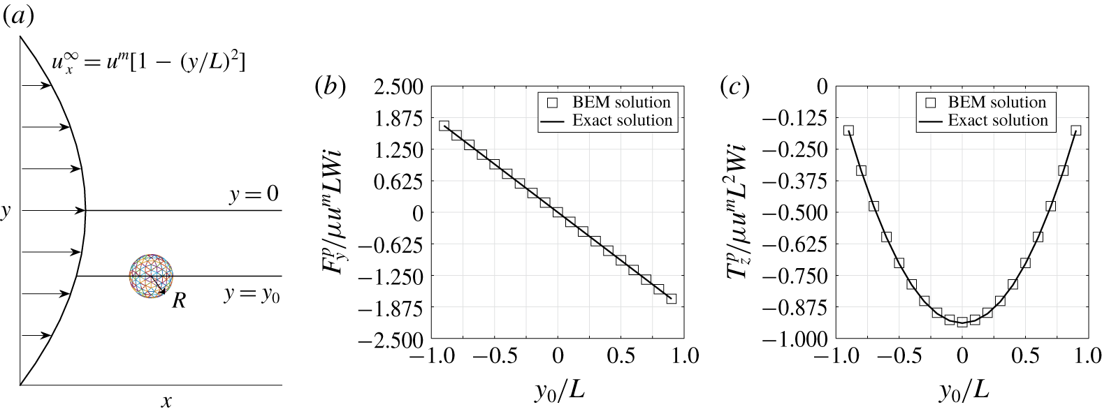
 $(x_{0},y_{0})$. Figure 3(a) shows a schematic of the set-up. Let the particle migrate at a velocity such that, at each point,
 $\boldsymbol{u}^{\infty }-\boldsymbol{U}=-\hat{\boldsymbol{e}}_{\boldsymbol{x}}-\hat{\boldsymbol{e}}_{\boldsymbol{y}}$ and
 $\unicode[STIX]{x1D734}-\unicode[STIX]{x1D74E}=\mathbf{0}$. We calculate the polymeric force and torque at various
 $y_{0}$ values using (2.26) and (2.27). The results compare well to our BEM simulation. Figure 3(b,c) shows the calculated
 $y$ component of the polymeric force and
 $z$ component of the polymeric torque. All other components are identically zero.
3.3 Spheroids under shear flow in a second-order fluid
We consider two different types of spheroids (prolate and oblate) that freely rotate under shear flow in a viscoelastic fluid. In previous experimental and theoretical studies, it was observed that such particles experience distinct orientation regimes at different shear rates. At relatively low shear rates with  $Wi\ll 0.1$, where
 $Wi$ is defined as
 $Wi=\unicode[STIX]{x1D713}_{1}\dot{\unicode[STIX]{x1D6FE}}/\unicode[STIX]{x1D707}$, the rotational behaviour of both prolate and oblate particles will be similar to those in Newtonian fluids due to the weak viscoelastic effect present in the system. A gradual transition in rotational behaviour is experimentally observed when the shear rate is increased
 $(Wi=0.1-1)$. Prolates tend to perform a log-rolling motion with the long axis aligned with the vorticity direction of the flow, while oblates or disk-shaped particles perform a tumbling motion with the short axis perpendicular to the vorticity axis (Gauthier et al. Reference Gauthier, Goldsmith and Mason1971; Bartram et al. Reference Bartram, Goldsmith and Mason1975; Johnson, Salem & Fuller Reference Johnson, Salem and Fuller1990; Gunes et al. Reference Gunes, Scirocco, J. and Vermant2008). At even higher shear rates (
 $Wi>O(1)$), Gunes et al. (Reference Gunes, Scirocco, J. and Vermant2008) reported that prolates will reorient the long axis along the flow direction when they are in a fluid with both high elasticity and shear-thinning. However, this reorientation transition is not observed when shear-thinning is absent even at extreme shear rates (
 $\dot{\unicode[STIX]{x1D6FE}}>200~\text{s}^{-1},Wi>30$). Bartram et al. (Reference Bartram, Goldsmith and Mason1975) reported that the reorientation state is metastable in Boger fluids (i.e. no shear-thinning) and the particle will perform log-rolling once subject to any perturbation such as a Brownian force or an imperfect flow field.
A previous theoretical study by Leal (Reference Leal1975) employing the slender-body approximation ( $A_{R}\rightarrow \infty$) predicted the reorientation transition for slender rods. The critical shear rate
 $\dot{\unicode[STIX]{x1D6FE}_{c}}$ for the reorientation to occur on a slender rod is predicted to be (Leal Reference Leal1975; Gunes et al. Reference Gunes, Scirocco, J. and Vermant2008)
 $$\begin{eqnarray}\dot{\unicode[STIX]{x1D6FE}_{c}}=\frac{16}{A_{R}}\left(\frac{\unicode[STIX]{x1D707}}{4\unicode[STIX]{x1D713}_{1}-\unicode[STIX]{x1D713}_{2}}\right).\end{eqnarray}$$
However, the critical shear rate of this transition does not quantitatively match experimental observations by Gunes et al. (Reference Gunes, Scirocco, J. and Vermant2008) on finite-aspect-ratio particles.
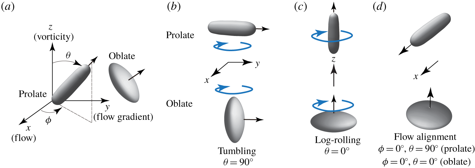
(a) Schematic of the particle orientation angles  $\unicode[STIX]{x1D719}$ and
 $\unicode[STIX]{x1D703}$ for prolate and oblate particles. The orientation vector for a prolate is along its long axis, while the vector for an oblate is along its short axis (arrows shown in the plot). (b–d) Schematic of possible rotation regimes for prolate and oblate particles. Tumbling refers to two-dimensional rotation in the
 $x$–
 $y$ plane (
 $\unicode[STIX]{x1D703}=90^{\circ }$), while log-rolling refers to two-dimensional rotation along the vorticity axis (
 $\unicode[STIX]{x1D703}=0^{\circ }$). Flow alignment for a prolate refers to alignment in the
 $x$ direction (
 $\unicode[STIX]{x1D703}=90^{\circ },\unicode[STIX]{x1D719}=0^{\circ }$). For an oblate, the alignment direction vector is the vorticity axis (
 $\unicode[STIX]{x1D703}=0^{\circ }$,
 $\unicode[STIX]{x1D719}=0^{\circ }$).

In this study, equations (2.26) and (2.27) are employed to investigate three-dimensional particle orientations in shear flow. The flow field is defined by
 $$\begin{eqnarray}u_{x}^{\infty }=\frac{y}{L},\quad u_{y}^{\infty }=u_{z}^{\infty }=0,\end{eqnarray}$$
where the shear rate of the flow is  $\dot{\unicode[STIX]{x1D6FE}}=\unicode[STIX]{x2202}u_{x}^{\infty }/\unicode[STIX]{x2202}y=1/L$. Similar to the experiments in Gunes et al. (Reference Gunes, Scirocco, J. and Vermant2008), we set the aspect ratio to be
 $A_{R}=3.8$ for both oblate and prolate particles. The particle orientation angles
 $\unicode[STIX]{x1D719}$ and
 $\unicode[STIX]{x1D703}$ are defined based on the direction of the particle’s major axis as shown in figure 2(a). Therefore, the transition of orientation regimes can be captured solely by
 $\unicode[STIX]{x1D703}$: for example, log-rolling of prolate particles corresponds to
 $\unicode[STIX]{x1D703}=0^{\circ }$, while tumbling of oblate particles in the
 $x$–
 $y$ plane corresponds to
 $\unicode[STIX]{x1D703}=90^{\circ }$. Figure 2(b–d) shows the schematics of various possible rotation modes for prolate and oblate particles. We set the initial orientations of the particle at
 $\unicode[STIX]{x1D703}_{0}=45^{\circ }$ and
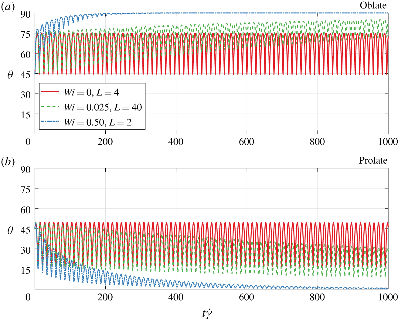
 $\unicode[STIX]{x1D719}_{0}=10^{\circ }$. Figure 4(a,b) shows the temporal evolution of angle
 $\unicode[STIX]{x1D703}$ under various shear rates, described by Weissenberg number
 $Wi=\unicode[STIX]{x1D713}_{1}\dot{\unicode[STIX]{x1D6FE}}/\unicode[STIX]{x1D707}$. In Newtonian flows (
 $Wi=0$), both particles perform the Jeffery orbit, i.e. a tumbling motion without any drift in
 $\unicode[STIX]{x1D703}$ observed. When viscoelasticity is present at a very low shear rate (
 $Wi=0.025$), the evolution in
 $\unicode[STIX]{x1D703}$ is similar to the Newtonian case, with a slight deviation observed in the later part of the simulation. As we increase the shear rate (
 $Wi=0.50$), a significant drift in
 $\unicode[STIX]{x1D703}$ is observed for both particles. The oblate drifts towards the tumbling state in the
 $x$–
 $y$ plane (
 $\unicode[STIX]{x1D703}=90^{\circ }$) while the prolate drifts towards the log-rolling state (
 $\unicode[STIX]{x1D703}=0^{\circ }$). We find that, as long as prolate particles do not start in the
 $x$–
 $y$ plane (
 $\unicode[STIX]{x1D703}=90^{\circ }$), the long-time configuration (
 $t\rightarrow \infty$) will always be the log-rolling state (
 $\unicode[STIX]{x1D703}=0^{\circ }$), consistent with the experimental observations of Bartram et al. (Reference Bartram, Goldsmith and Mason1975) for particles in Boger fluids.
(a) Set-up for a spherical particle in a pressure-driven flow. (b) Non-dimensionalized polymeric force in the  $y$ direction for different values of
 $y_{0}$. (c) Non-dimensionalized polymeric torque in the
 $z$ direction for different values of
 $y_{0}$. The parameters are
 $R=1$,
 $L=10$,
 $u^{m}=1$,
 $\unicode[STIX]{x1D707}=1$,
 $\unicode[STIX]{x1D713}_{1}=1$ and
 $Wi=0.1$. The Weissenberg number is defined by
 $Wi=\unicode[STIX]{x1D713}_{1}u^{m}/L\unicode[STIX]{x1D707}$.

(a) Plot of  $\unicode[STIX]{x1D703}$ versus time
 $t$ for an oblate particle in a simple shear flow
 $u_{x}^{\infty }=y/L$. (b) Plot of
 $\unicode[STIX]{x1D703}$ versus time
 $t$ for a prolate particle in shear flow
 $u_{x}^{\infty }=y/L$. The common parameters are
 $R=1$,
 $A_{R}=3.8$,
 $\unicode[STIX]{x1D707}=1$ and
 $\unicode[STIX]{x1D713}_{1}=1$. The initial orientations are
 $\unicode[STIX]{x1D703}_{0}=45^{\circ }$ and
 $\unicode[STIX]{x1D719}_{0}=10^{\circ }$. The Weissenberg number in the shear flow is defined as
 $Wi=\unicode[STIX]{x1D713}_{1}\dot{\unicode[STIX]{x1D6FE}}/\unicode[STIX]{x1D707}$. The case of
 $Wi=0$ corresponds to a Newtonian flow with
 $\unicode[STIX]{x1D713}_{1}=0$.

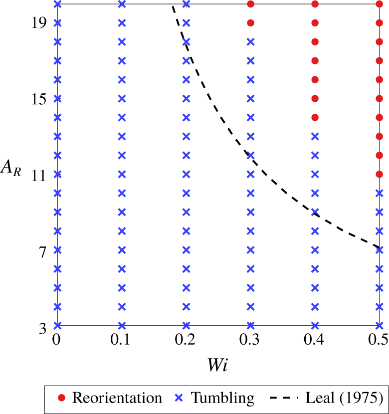
The phase diagram of prolate orientation modes for different Weissenberg numbers  $Wi\equiv \unicode[STIX]{x1D713}_{1}\dot{\unicode[STIX]{x1D6FE}}/\unicode[STIX]{x1D707}$ and particle aspect ratios
 $A_{R}$. The dashed line represents the critical
 $Wi$ predicted by (3.6) with
 $\unicode[STIX]{x1D713}_{1}=-2\unicode[STIX]{x1D713}_{2}$. The
 $\unicode[STIX]{x1D703}$ angle is fixed at 90°. Reorientation stands for flow alignment (
 $\unicode[STIX]{x1D703}=90^{\circ },\unicode[STIX]{x1D719}=0^{\circ }$), and tumbling represents
 $\unicode[STIX]{x1D703}=90^{\circ }$ with periodically changing
 $\unicode[STIX]{x1D719}$. The other parameters are
 $R=1$,
 $\unicode[STIX]{x1D707}=1$ and
 $\unicode[STIX]{x1D713}_{1}=1$.

When prolate particles are restricted to lie in the  $x$–
 $y$ plane (metastable regime), the particles can either tumble or align along the flow direction (
 $\unicode[STIX]{x1D703}=90^{\circ },\unicode[STIX]{x1D719}=0^{\circ }$). Figure 5 shows the phase diagram of prolate orientation modes under various flow conditions
 $Wi$ and particle aspect ratios
 $A_{R}$. We observe a transition from tumbling to reorientation (i.e. flow alignment) above a critical shear rate, with no transition occurring for aspect ratios
 $3\leqslant A_{R}\leqslant 6$ under the tested conditions. The critical shear rate predicted by (3.6) (dashed line in figure 5) is quantitatively inconsistent with our results especially in the low-
 $A_{R}$ regime. The equation will provide better consistency (not shown here) at extreme
 $A_{R}$ such as
 $A_{R}=100$, indicating the limited applicability of (3.6) to slender-body systems. The observations here are in qualitative agreement with previous studies by Bartram et al. (Reference Bartram, Goldsmith and Mason1975), Johnson et al. (Reference Johnson, Salem and Fuller1990) and Gunes et al. (Reference Gunes, Scirocco, J. and Vermant2008). Quantitatively, Gunes et al. (Reference Gunes, Scirocco, J. and Vermant2008) observed that transition occurs for
 $A_{R}=3.8$ in the regime where
 $Wi>1$. In such a flow regime the second-order fluid model will lose its validity and therefore a quantitative discussion of the phenomenon would require extending the current model to more general conditions as well as considering more complex physics such as shear-thinning effects.
3.4 General ellipsoids in quadratic flows
We consider general ellipsoids (sphere, prolate, oblate and prolate-like ellipsoid) in a second-order fluid under a parabolic profile defined by (3.5). We follow the particle geometry definitions in § 3.1. We investigate the effect of particle orientation, position and morphology on particle migration. We also examine the translational and rotational trajectories in a quadratic flow. The common parameters are  $R=1$,
 $L=4$,
 $\unicode[STIX]{x1D707}=1$ and
 $\unicode[STIX]{x1D713}_{1}=1$. We vary the maximum flow velocity
 $u^{m}$, and hence can vary the flow Weissenberg number
 $Wi\equiv \unicode[STIX]{x1D713}_{1}u^{m}/L\unicode[STIX]{x1D707}$.
3.4.1 Effect of particle orientation, position and morphology
We first study cross-stream particle migration under different particle orientations. We set the particle aspect ratio to be  $A_{R}=3$ and their initial position at
 $(x_{0},y_{0})=(0,-3.5)$. We calculate the particle lateral velocity
 $U_{y}$ and rotational velocity
 $\unicode[STIX]{x1D714}_{z}$ at different particle orientations
 $\unicode[STIX]{x1D719}$ and
 $\unicode[STIX]{x1D703}$. For lateral migration velocity
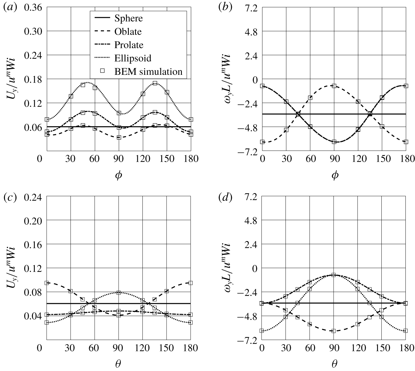
 $U_{y}$, it can be seen in figure 6(a) that all non-spherical particles show similar behaviour with respect to
 $\unicode[STIX]{x1D719}$, with the fastest migration occurring at
 $\unicode[STIX]{x1D719}=45^{\circ }$ and 135°. The prolate-like ellipsoid shows the fastest lateral migration among all the particles. Figure 6(c) shows the lateral migration velocity at various
 $\unicode[STIX]{x1D703}$ angles. The prolate and prolate-like ellipsoids show maximum
 $U_{y}$ at
 $\unicode[STIX]{x1D703}=90^{\circ }$ and minimum at
 $\unicode[STIX]{x1D703}=0^{\circ }$, since particles in these configurations yield the largest and smallest span along the shear-gradient direction (
 $y$ direction), respectively.. The oblate shows the opposite behaviour due to its morphology.
For the rotational dynamics, figures 6(b) and 6(d) show the rotational velocity  $\unicode[STIX]{x1D714}_{z}$ at various
 $\unicode[STIX]{x1D719}$ and
 $\unicode[STIX]{x1D703}$ angles, respectively. In figure 6(b) the prolate and prolate-like ellipsoids perform nearly identical sinusoidal behaviour in rotational velocity
 $\unicode[STIX]{x1D714}_{z}$ throughout the tested range of
 $\unicode[STIX]{x1D719}$, with the fastest rotation appearing at
 $\unicode[STIX]{x1D719}=90^{\circ }$. The oblate shows a 90° phase lag in
 $\unicode[STIX]{x1D714}_{z}$ compared to that of the prolate and ellipsoid. In figure 6(d), the rotational velocity
 $\unicode[STIX]{x1D714}_{z}$ decreases for prolate and ellipsoid particles as the angle
 $\unicode[STIX]{x1D703}$ increases, due to the fact that the particle’s moment of inertia in the vorticity direction (
 $z$ direction) increases. The opposite trend in
 $\unicode[STIX]{x1D703}$ is observed for the oblate particle due to the same physics.
We next study the particle migration behaviour at different positions in the flow. We first fix the particle orientation at  $\unicode[STIX]{x1D703}=90^{\circ }$,
 $\unicode[STIX]{x1D719}=45^{\circ }$ and calculate the particle lateral velocity
 $U_{y}$ and rotational velocity
 $\unicode[STIX]{x1D714}_{z}$ at various initial positions
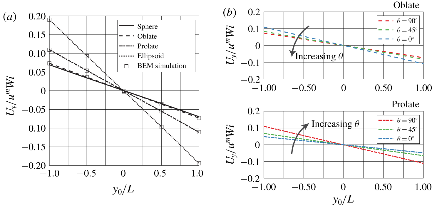
 $y_{0}$. Figure 7(a) shows that all particles tend to migrate towards the centre of the flow profile regardless of their position in the flow. The lateral velocity
 $U_{y}$ and rotational velocity
 $\unicode[STIX]{x1D714}_{z}$ show a linear dependence with respect to
 $y_{0}$. The prolate-like ellipsoid shows the most significant lateral migration among all particles. A similar linear trend of
 $U_{y}$ is also observed as we change the
 $\unicode[STIX]{x1D703}$ orientation, as shown in figure 7(b).
(a) Non-dimensionalized migration velocity  $U_{y}$ under different particle orientation angles
 $\unicode[STIX]{x1D719}$ in a pressure-driven flow defined by (3.5). (b) Non-dimensionalized particle rotational velocity
 $\unicode[STIX]{x1D714}_{z}$ under different particle orientations
 $\unicode[STIX]{x1D719}$. In (a) and (b) the particle
 $\unicode[STIX]{x1D703}$ angle is set to be 90° (in the
 $x$–
 $y$ plane). (c) Non-dimensionalized particle migration velocity
 $U_{y}$ under different particle orientations
 $\unicode[STIX]{x1D703}$. (d) Non-dimensionalized particle rotational velocity
 $\unicode[STIX]{x1D714}_{z}$ under different particle orientations
 $\unicode[STIX]{x1D703}$. In (c) and (d) the particle
 $\unicode[STIX]{x1D719}$ angle is set to be 0° (along the
 $x$ direction). The common parameters are
 $R=1$,
 $A_{R}=3$,
 $L=4$,
 $u^{m}=1$,
 $\unicode[STIX]{x1D707}=1$,
 $\unicode[STIX]{x1D713}_{1}=1$ and
 $Wi=0.25$. The particle’s position is
 $(x_{0},y_{0})=(0,-3.5)$. The angle
 $\unicode[STIX]{x1D719}$ is defined between 0° and 180° due to particle symmetry.

(a) Non-dimensionalized migration velocity  $U_{y}$ in a pressure-driven flow defined by (3.5) for cross-stream positions
 $y_{0}$. The particle orientations are
 $\unicode[STIX]{x1D719}=45^{\circ }$,
 $\unicode[STIX]{x1D703}=90^{\circ }$. (b) Non-dimensionalized migration velocity
 $U_{y}$ of the oblate and prolate particle for cross-stream positions
 $y_{0}$ at
 $\unicode[STIX]{x1D719}=45^{\circ }$ and various
 $\unicode[STIX]{x1D703}$ orientations. The common parameters are
 $A_{R}=3$,
 $R=1$,
 $L=4$,
 $u^{m}=1$,
 $\unicode[STIX]{x1D707}=1$,
 $\unicode[STIX]{x1D713}_{1}=1$ and
 $Wi=0.25$.

To explain these observations, we refer to the scaling analysis by Leshansky et al. (Reference Leshansky, Bransky, Korin and Dinnar2007). In their paper, Leshansky et al. (Reference Leshansky, Bransky, Korin and Dinnar2007) proposed that the polymeric force on a particle of characteristic radius  $R$ scales linearly with the normal stress gradients as
 $F_{y}^{p}\sim R^{3}\unicode[STIX]{x1D713}_{1}(\unicode[STIX]{x2202}/\unicode[STIX]{x2202}y)(\unicode[STIX]{x2202}u_{x}^{\infty }/\unicode[STIX]{x2202}y)^{2}|_{y=y_{0}}$. When force-free, the polymeric force should balance the Stokes drag
 $F_{y}^{D}$ in the opposite direction:
 $F_{y}^{D}\sim -\unicode[STIX]{x1D707}RU_{y}$. The lateral migration velocity
 $U_{y}$ should thus scale as
 $U_{y}\sim (\unicode[STIX]{x1D713}_{1}R^{2}(u^{m})^{2}/\unicode[STIX]{x1D707})\,y_{0}/L^{4}$, which shows a linear dependence on
 $y_{0}$ as in our calculations.
We next extend the scaling analysis above to study the influence of particle shape on the particle mobility. We define the proportionality constant for the  $U_{y}$ scaling relation to be the mobility constant
 $M_{D}$:
 $$\begin{eqnarray}U_{y}=M_{D}\frac{\unicode[STIX]{x1D713}_{1}R^{2}{u^{m}}^{2}}{\unicode[STIX]{x1D707}}\frac{y_{0}}{L^{4}}=M_{D}WiR^{2}u^{m}\frac{y_{0}}{L^{3}},\end{eqnarray}$$
where  $Wi$ is the Weissenberg number, defined as
 $Wi=\unicode[STIX]{x1D713}_{1}u^{m}/L\unicode[STIX]{x1D707}$. We apply this relation to calculate the mobility
 $M_{D}$ for different particle shapes.
Here we specifically investigate two different sets of particle orientations,  $\unicode[STIX]{x1D703}=90^{\circ },\unicode[STIX]{x1D719}=45^{\circ }$ and
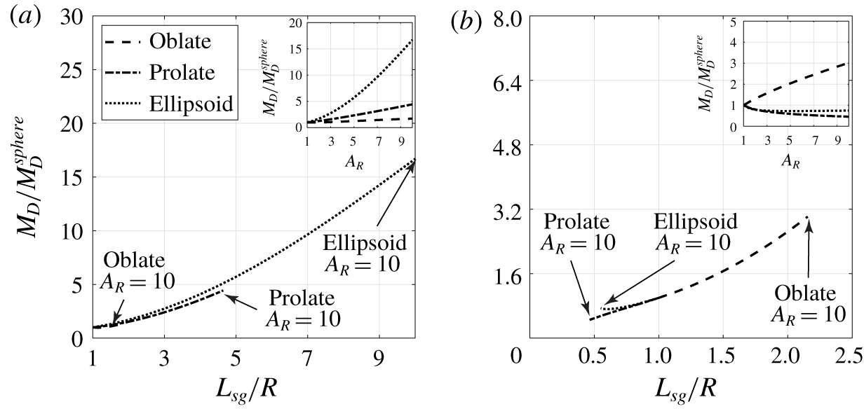
 $\unicode[STIX]{x1D703}=0^{\circ },\unicode[STIX]{x1D719}=45^{\circ }$, and the results are presented in figure 8(a,b). The insets of both panels show the particle relative mobility with respect to a sphere,
 $M_{D}/M_{D}^{sphere}$, at different particle aspect ratios
 $A_{R}$. When
 $\unicode[STIX]{x1D703}=90^{\circ }$, all three types of particles have higher mobility at higher
 $A_{R}$ and the prolate-like ellipsoid shows the most significant increase in the mobility among the three. In the case of
 $\unicode[STIX]{x1D703}=0^{\circ }$, only the oblate gains higher mobility at higher
 $A_{R}$, while the prolate and ellipsoid show decreasing mobility. However, when we plot the mobility data against the longest possible particle axis length in the shear gradient direction
 $L_{sg}$, the mobility curves for all three particles collapse onto one major curve as shown in figure 8. This indicates that the effective length spanned along the velocity gradient is the major factor that affects the particle mobility in the flow. In the case when
 $\unicode[STIX]{x1D703}=90^{\circ }$, the major axis length of the particle acts as the determining factor for the migration velocity in the velocity gradient direction, while in the case of
 $\unicode[STIX]{x1D703}=0^{\circ }$, the shorter axes of prolate and ellipsoid and the long axis of oblate will be the dominant factors. This also explains the decreasing trend in mobility with respect to
 $A_{R}$ for prolate and ellipsoid when
 $\unicode[STIX]{x1D703}=0^{\circ }$. For
 $0^{\circ }<\unicode[STIX]{x1D703}<90^{\circ }$, the dominant length will be a mixture of long and short particle axes.
3.4.2 Particle migration trajectories
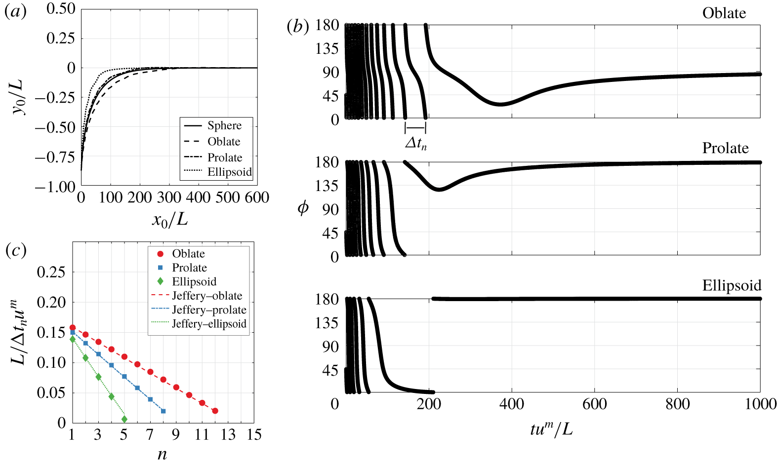
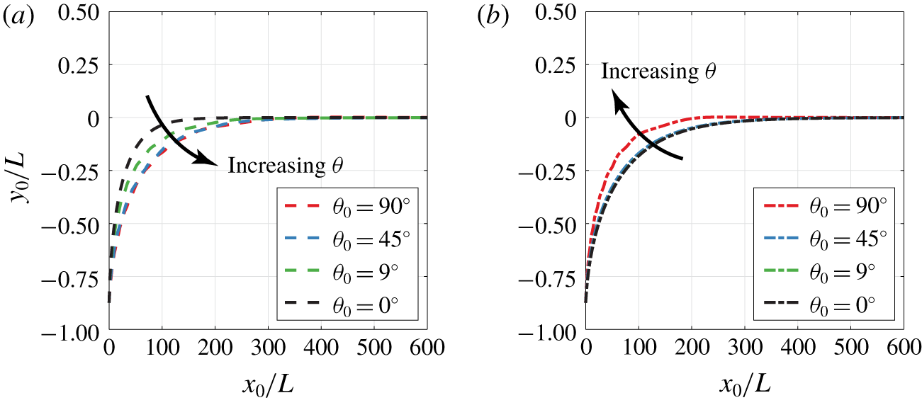
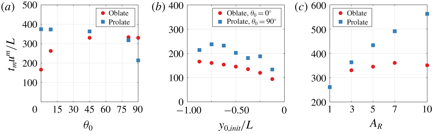
In figure 9(a,b), we first restrict the particle orientation in the flow–shear gradient plane ( $\unicode[STIX]{x1D703}=90^{\circ }$) and track the trajectories of tumbling particles in a pressure-driven flow as they migrate to the flow centre. The particles are released at
 $(x_{0},y_{0})=(0,-3.5)$ with an initial orientation
 $\unicode[STIX]{x1D719}_{0}=$ 45°. It can be seen from figure 9(a) that the prolate-like ellipsoids and the oblate particles exhibit the fastest and the slowest migration speeds, respectively. Particles tend to stay near the flow centre once they reach the region since the polymeric force is zero. Figure 9(b) shows the evolution of particle orientation angle
 $\unicode[STIX]{x1D719}$ with respect to the dimensionless time
 $tu^{m}/L$. The non-spherical particles perform a clockwise tumbling motion during migration and attain a steady orientation once they reach the flow centre. At the flow centre, the particles align their longest axis with the flow (
 $\unicode[STIX]{x1D719}=0^{\circ }$ for prolate and prolate-like ellipsoid,
 $\unicode[STIX]{x1D719}=90^{\circ }$ for oblate). These observations qualitatively agree with the results from D’Avino et al. (Reference D’Avino, Hulsen, Greco and Maffettone2019) when particles are restricted to the
 $x$–
 $y$ plane.
(a) The relative particle mobility  $M_{D}/M_{D}^{sphere}$ as a function of the particle’s longest semi-axis length in the shear gradient direction
 $L_{sg}$ at
 $\unicode[STIX]{x1D703}=90^{\circ },\unicode[STIX]{x1D719}=45^{\circ }$. Here,
 $L_{sg}$ is the longest axis length for all three particle families studied, where
 $L_{sg}=a$ for prolate and ellipsoid particles and
 $L_{sg}=b$ for oblate particles. (b) The relative particle mobility
 $M_{D}/M_{D}^{sphere}$ as a function of the particle’s longest semi-axis length in the shear gradient direction
 $L_{sg}$ at
 $\unicode[STIX]{x1D703}=0^{\circ },\unicode[STIX]{x1D719}=45^{\circ }$. Here,
 $L_{sg}=b$ is the shortest axis length for the prolate particles, and
 $L_{sg}=b$ is the longest axis for oblate particles. For the prolate-like ellipsoids, we choose
 $L_{sg}$ as the average of the
 $b$ and
 $c$ axes. The insets in both plots show the relative particle mobility
 $M_{D}/M_{D}^{sphere}$ at different aspect ratios
 $A_{R}$. The common parameters are
 $y_{0}=-3.5$,
 $R=1$,
 $L=4$,
 $u^{m}=1$,
 $\unicode[STIX]{x1D707}=1$,
 $\unicode[STIX]{x1D713}_{1}=1$ and
 $Wi=0.25$.

(a) Particle trajectories in a pressure-driven flow. Particles are released at  $(x_{0},y_{0})=(0,-3.5)$ with initial orientation
 $\unicode[STIX]{x1D703}=90^{\circ }$,
 $\unicode[STIX]{x1D719}=45^{\circ }$ (i.e. in the
 $x$–
 $y$ plane). (b) Particle orientation
 $\unicode[STIX]{x1D719}$ with respect to the simulation time
 $t$. (c) The reciprocal of the time required for
 $n$th flip
 $1/\unicode[STIX]{x0394}t_{n}$ with respect to the flip count
 $n$. The simulation parameters are
 $R=1$,
 $L=4$,
 $A_{R}=3$,
 $u^{m}=1$,
 $\unicode[STIX]{x1D707}=1$,
 $\unicode[STIX]{x1D713}_{1}=1$ and
 $Wi=0.25$. Time is non-dimensionalized by the average shear rate
 $u^{m}/L$. The duration of the simulation is
 $tu^{m}/L=1000$.

In order to quantify the tumbling motion, we define  $n$ as the number of times a particle performs a 180° flip and
 $\unicode[STIX]{x0394}t_{n}$ as the time required for the
 $n$th flip to occur. The plot of
 $1/\unicode[STIX]{x0394}t_{n}$ with respect to
 $n$ for the three non-spherical particles is shown in figure 9(c). In general, particles will rotate at a slower rate as they approach the flow centre. The prolate-like ellipsoid achieved the least number of flips (
 $n=5$) due to its fastest migration towards the flow centre. The oblate, on the other hand, spent more time in the off-centre region and therefore shows the highest number of flips (
 $n=12$) among the three particles. Jeffery (Reference Jeffery1922) proposed that, for a general ellipsoidal particle in a Newtonian fluid under shear rate
 $\dot{\unicode[STIX]{x1D6FE}}$, the tumbling period
 ${\mathcal{T}}^{J}$ of the particle follows
 $$\begin{eqnarray}{\mathcal{T}}^{J}=\frac{2\unicode[STIX]{x03C0}}{\dot{\unicode[STIX]{x1D6FE}}}\left(A_{R}+\frac{1}{A_{R}}\right).\end{eqnarray}$$
We sample the shear rate at the averaged  $y$ position during each flip to estimate the local Jeffery orbit period. The calculated half-period data are also shown in figure 9(c) for comparison. The results show that the tumbling behaviour of the three non-spherical particles in the off-centre region of the flow are in good agreement with the Jeffery orbits, with only less than 4 % of error from
 ${\mathcal{T}}^{J}$. Deviation from Jeffery orbit is only observed as the particles approach the flow centre, where the quadratic part of the flow dominates the particle motion. The results indicate that, under the above flow condition, the polymeric effect does not greatly alter the rotation dynamics from the Newtonian behaviour.
(a) Plot of oblate  $\unicode[STIX]{x1D703}$ trajectory with respect to simulation time
 $t$ under various initial orientations
 $\unicode[STIX]{x1D703}_{0}$. (b) Plot of prolate
 $\unicode[STIX]{x1D703}$ trajectory with respect to simulation time
 $t$ under various initial orientations
 $\unicode[STIX]{x1D703}_{0}$. The common parameters are
 $R=1$,
 $L=4$,
 $A_{R}=3$,
 $u^{m}=1$,
 $\unicode[STIX]{x1D707}=1$,
 $\unicode[STIX]{x1D713}_{1}=1$ and
 $Wi=0.25$. The particles are released at
 $(x_{0},y_{0})=(0,-3.5)$. Time is non-dimensionalized by the average, inverse shear rate
 $L/u^{m}$. The duration of the simulation is
 $tu^{m}/L=1000$.

We next explore the effect of initial  $\unicode[STIX]{x1D703}$ orientation on their migration trajectories. In this test, particles are released at
 $(x_{0},y_{0})=(0,-3.5)$ and at various initial
 $\unicode[STIX]{x1D703}$ orientations
 $\unicode[STIX]{x1D703}_{0}$ with the initial
 $\unicode[STIX]{x1D719}$ angle fixed at
 $45^{\circ }$. In figure 10(a,b) we report the
 $\unicode[STIX]{x1D703}$ trajectories of oblate and prolate particles. When the particle initial
 $\unicode[STIX]{x1D703}_{0}$ orientation lies exactly at
 $\unicode[STIX]{x1D703}_{0}=0^{\circ }$ or
 $\unicode[STIX]{x1D703}_{0}=90^{\circ }$, no drift in
 $\unicode[STIX]{x1D703}$ is observed throughout the simulation. When
 $\unicode[STIX]{x1D703}_{0}$ lies between 0° and 90°, both particles show a drift in
 $\unicode[STIX]{x1D703}$ towards their favoured orientation – the oblate drifts towards
 $\unicode[STIX]{x1D703}=90^{\circ }$ (tumbling in figure 2b) and the prolate drifts towards
 $\unicode[STIX]{x1D703}=0^{\circ }$ (log-rolling in figure 2c). In both cases, these favoured orientations correspond to the situation when the longest particle semi-axis aligns with the vorticity axis of the flow. Metastable states correspond to
 $\unicode[STIX]{x1D703}_{0}=0^{\circ }$ for oblates (log-rolling in figure 2c) and
 $\unicode[STIX]{x1D703}_{0}=90^{\circ }$ for prolates (tumbling in figure 2b).
Figure 11 shows how the initial orientation angle  $\unicode[STIX]{x1D703}$ alters the position of the particle as it moves towards the flow centre. Generally, the migration speed is fastest when the particle’s initial orientation spans the largest distance in the shear gradient direction (i.e.
 $\unicode[STIX]{x1D703}_{0}=0^{\circ }$ for oblate,
 $\unicode[STIX]{x1D703}_{0}=90^{\circ }$ for prolate). This state corresponds to the metastable configuration for both prolates and oblates. Lastly, figure 12 plots how the migration time
 $t_{m}$ towards the flow centre varies with initial orientation
 $\unicode[STIX]{x1D703}_{0}$, initial position
 $y_{0,init}$ and aspect ratio
 $A_{R}$. In these plots,
 $t_{m}$ is defined as the time it takes for the particle to reach
 $y_{0}<0.01L$ from the flow centre. In figure 12(a), both oblate and prolate particles have a slight variation in
 $t_{m}$ when
 $\unicode[STIX]{x1D703}_{0}$ is close to their stable orientation. A steep drop in
 $t_{m}$ is observed near the metastable orientation. Figure 12(b) shows the plot of
 $t_{m}$ with respect to various initial
 $y_{0,init}$. The initial
 $\unicode[STIX]{x1D703}$ orientation was set to be 0° and 90° for oblates and prolates, respectively. Oblate particles show a monotonic decrease in
 $t_{m}$ with decreasing
 $y_{0,init}$. On the other hand, prolate particles show a non-monotonic trend in
 $t_{m}$, mainly due to the fact that tumbling motion (thus change in
 $\unicode[STIX]{x1D719}$ angle) also plays a role in their migration dynamics. We note that such effects do not occur for oblates with
 $\unicode[STIX]{x1D703}_{0}=0^{\circ }$ since different
 $\unicode[STIX]{x1D719}$ angles correspond to the same state of orientation. Figure 12(c) shows the variation of
 $t_{m}$ with respect to particle aspect ratio
 $A_{R}$ for prolate and oblate particles. Both particles show longer migration time with increasing
 $A_{R}$. Prolate particles always transition into a log-rolling state and thus have migration time
 $t_{m}$ increasing monotonically with
 $A_{R}$. On the other hand, oblate particles tend to perform tumbling motion (
 $\unicode[STIX]{x1D703}=90^{\circ }$) during their migration. The migration time is affected by both long and short axes, and therefore the trend is not monotonic.
(a) Plot of oblate migration trajectories from various  $\unicode[STIX]{x1D703}_{0}$. (b) Plot of prolate migration trajectories from various
 $\unicode[STIX]{x1D703}_{0}$. The particles are released at
 $(x_{0},y_{0})=(0,-3.5)$. The common parameters are
 $R=1$,
 $L=4$,
 $A_{R}=3$,
 $u^{m}=1$,
 $\unicode[STIX]{x1D707}=1$,
 $\unicode[STIX]{x1D713}_{1}=1$ and
 $Wi=0.25$. The simulation duration is
 $tu^{m}/L=1000$.

(a) The migration time  $t_{m}$ required for aspect ratio
 $A_{R}=3$ oblate and prolate particles to reach
 $y_{0}<0.01L$ from different initial
 $\unicode[STIX]{x1D703}$ orientations. Particles are released at
 $(x_{0},y_{0})=(0,-3.5)$ with initial
 $\unicode[STIX]{x1D719}_{0}=45^{\circ }$. (b) The migration time
 $t_{m}$ required for
 $A_{R}=3$ oblate and prolate particles to reach
 $y_{0}<0.01L$ from different lateral positions
 $y_{0,init}$. The initial
 $\unicode[STIX]{x1D703}$ orientation is set to be
 $\unicode[STIX]{x1D703}_{0}=0^{\circ }$ and
 $\unicode[STIX]{x1D703}_{0}=90^{\circ }$ for oblates and prolates, respectively. Initial
 $\unicode[STIX]{x1D719}_{0}$ is set at 45°. (c) The migration time
 $t_{m}$ required for oblate and prolate particles to reach
 $y_{0}<0.01L$ for different particle aspect ratios. Particles were released at
 $(x_{0},y_{0})=(0,-3.5)$ with initial orientation
 $\unicode[STIX]{x1D703}_{0}=45^{\circ },\unicode[STIX]{x1D719}_{0}=45^{\circ }$. The common parameters are
 $R=1$,
 $L=4$,
 $u^{m}=1$,
 $\unicode[STIX]{x1D707}=1$,
 $\unicode[STIX]{x1D713}_{1}=1$ and
 $Wi=0.25$.

4 Conclusion and future directions
We studied the dynamics of non-spherical particles in an inertialess, steady flow of a second-order fluid. The assumption of  $\unicode[STIX]{x1D713}_{1}=-2\unicode[STIX]{x1D713}_{2}$ allows us to reduce the fluid dynamics to a Stokes flow with a modified total pressure. By utilizing a multipole expansion, we derived an analytical solution for the polymeric force and torque on an arbitrarily shaped particle in a general quadratic flow field (i.e. quadratic plus linear flow in an unbound domain). The solutions are in good agreement with previous studies on spherical particle dynamics in viscoelastic flows as well as our boundary element simulations. We also verified that our theory can qualitatively capture the experimentally observed orientation transitions of spheroids under various flow conditions.
We applied our model to investigate the dynamics of spheres, spheroids (oblate and prolate) and ellipsoids in a slit-like pressure-driven flow of second-order fluid. In general, the particles slowly migrate to the centre of the pressure-driven flow, with their dynamics governed by the position, orientation and particle morphology. We develop scaling theories to quantify how the particle shape affects the migration velocity. The length  $L_{sg}$ spanned by the particles in the velocity gradient direction determines the lift velocity for a wide range of particle family shapes. Our trajectory studies show that spheroidal particles slowly adjust their orientation towards a favoured configuration (e.g. log-rolling for prolates, tumbling for oblates). The effect of initial orientation, initial position and particle aspect ratio on the migration time is also identified in this paper.
This work provides a preliminary understanding of non-spherical particle dynamics in viscoelastic flows from an analytical standpoint. For future directions, investigations towards more general conditions (e.g.  $\unicode[STIX]{x1D713}_{1}\neq -2\unicode[STIX]{x1D713}_{2}$) are necessary for a better understanding of particle dynamics in a viscoelastic flow. It is also our interest to investigate more complicated systems such as wall-bounded flows and three-dimensional flows to understand the particle dynamics in realistic systems such as microfluidic platforms. Experimental studies on particle dynamics in viscoelastic flow will also provide insight on the validity of the developed model to real systems.
Acknowledgements
The authors would like to thank Professors S. Kim and A. Ardekani for illuminating discussions, as well as suggestions from the anonymous reviewers, which greatly improved the manuscript. This work used the Extreme Science and Engineering Discovery Environment (XSEDE), which is supported by National Science Foundation grant numbers CTS190055 and CHE190089.
Declaration of interests
The authors report no conflict of interest.