2·1. Commutative Groups of Prime Power Order

As mentioned before, our results can still be applied when arbitrary finite commutative p-groups $B_j=\bigoplus_{i=1}^{K_j} (\mathbb{Z}/p^{\beta_{j,i}} \mathbb{Z})$ replace the cyclic p-groups $\mathbb{Z}/p^{\beta_j} \mathbb{Z}$ as codomains. One just has to use the coordinate projections $\pi_k\,{:}\,\bigoplus_{i=1}^{K_j} (\mathbb{Z}/p^{\beta_{j,i}}\mathbb{Z}) {{\rightarrow}} \mathbb{Z}/p^{\beta_{j,k}} \mathbb{Z}$ first (as already explained in [ Reference Clark and Schauz5 , Rem. 1·8]), to define the functions

\[f_{j,k}\,{: \! =}\,\pi_k \circ f_j \quad \text{with} \quad \mathrm{fdeg}(f_{j,k}) \leq \mathrm{fdeg}(f_j) \leq d_j\,.\]

Then our results can be applied to those $f_{j,k}$ and the degree restrictions $\mathrm{fdeg}(f_{j,k}) \leq d_j$ , with the outcome interpreted in terms of the $f_j$ .

If, for instance, Corollary 1·4 is applied in this way, then the parameter $\mathcal B$ takes the form $\mathcal B=\sum_{j=1}^r\bigl(d_j\sum_{k=1}^{K_j}(({p^{\beta_{j,k}} \! -1})/({p-1}))\bigr)$ , while the parameter $\mathcal A$ and the conclusion remain unchanged: still $\mathcal A\gt \mathcal B$ implies $\mathrm{ord}_p(\# Z_{A}(f_1,\dots,f_r)) \geq 1$ . This generalises Theorem 1·3, where $B_1= \dots =B_r=\bigoplus_{i=1}^{K} (\mathbb{Z}/p^{\beta_{i}} \mathbb{Z})$ , i.e., $\mathcal{B}=\sum_{j=1}^r d_j\sum_{k=1}^{K} (({p^{\beta_{k}} \! -1})/({p-1}))$ , and $A=\bigl(\bigoplus_{i=1}^m \mathbb{Z}/p^{\alpha_i}\mathbb{Z}\bigr)^N$ , i.e., $\mathcal{A}=N\sum_{i=1}^m (({p^{\alpha_i} \! -1})/({p-1}))$ .

2·2. Commutative Groups of Finite Order

Let $A,B_1,\dots,B_r$ be any nontrivial finite commutative groups. We write out the primes dividing $\# \left( A \times \prod_{i=1}^r B_i \right)$ as $\ell_1 \lt \cdots \lt \ell_s$ , and set

\[A[\ell_j^{\infty}]\,{: \! =}\,\bigl\{x \in A \mid \ell_j^k x = 0 \text{ for some } k\in\mathbb{Z}^+\bigr\}\,.\]

For each fixed $1 \leq j \leq r$ , we have a canonical $\mathbb{Z}$ -module injection

\[\prod_{h=1}^s B_j[\ell_h^{\infty}]^{A[\ell_h^{\infty}]} {{\rightarrow}} B_j^{\,A}\]

in which we send each vector $(g_{j,1},\dots,g_{j,s})$ of functions $g_{j,h}\,{:}\,A[\ell_h^{\infty}] {{\rightarrow}} B_j[\ell_h^{\infty}]$ to the identically named function

\begin{align*} (g_{j,1},\dots,g_{j,s})\;:\; A=\prod_{h=1}^sA[\ell_h^{\infty}] &\rightarrow B_j=\prod_{h=1}^sB_j[\ell_h^{\infty}]\\ (x_1,\dots,x_s) &\mapsto \bigl(g_{j,1}(x_1),\dots,g_{j,s}(x_s)\bigr)\,.\end{align*}

By [ Reference Clark and Schauz4 , cor. 3·14c and cor. 3·15], upon restriction to functions of finite functional degree, this yields a canonical isomorphism. Via identification, we have

\[\mathcal{F}(A,B_j) \,=\, \prod_{h=1}^s \mathcal{F}(A[\ell_h^{\infty}],B_j[\ell_h^{\infty}])\]

in which moreover $\mathrm{fdeg}((g_{j,1},\dots,g_{j,s})) = \max \{\mathrm{fdeg}(g_{j,h}) \mid 1 \leq h \leq s\}$ . In other words, a map $f_j\,{:}\,A {{\rightarrow}} B_j$ of finite functional degree is determined by its restrictions $g_{j,h}\,{: \! =}\,f_j|_{A[\ell_h^\infty]}\in B_j[\ell_h^{\infty}]^{A[\ell_h^{\infty}]}$ , and we may write

\[f_j=(g_{j,1},\dots,g_{j,s}) \quad \text{and} \quad \mathrm{fdeg}(f_j) = \max\bigl\{\mathrm{fdeg}(g_{j,h}) \mid 1 \leq h \leq s\bigr\}\,.\]

If we now consider r maps $f_j\,{:}\,A {{\rightarrow}} B_j$ , where $1 \leq j \leq r$ , then we get $s\times r$ primary component maps $g_{j,h}\,{:}\, A[\ell_h^{\infty}]{{\rightarrow}} B_j[\ell_h^{\infty}]$ , and it is immediate that

\[\# Z(f_1,\dots,f_r) \,=\, \prod_{h=1}^s \# Z(g_{1,h}\,,\dots,g_{r,h})\,.\]

So, with the previous Section 2·1, we obtain for each $1 \leq h \leq s$ a lower bound on $\mathrm{ord}_{\ell_h}\bigl(\# Z(f_1,\dots,f_r)\bigr)$ in terms of $A,B_1,\dots,B_r$ and $\mathrm{fdeg}(f_1),\dots,\mathrm{fdeg}(f_r)$ .

2·3. Polynomials over Rngs of Prime Power Order

Before [ Reference Clark and Schauz5 ], Ax–Katz type p-adic congruences on the solution set of a polynomial system over a finite rng were only known for finite commutative rings in which every ideal is principal [ Reference Ax2 , Reference Katz8 , Reference Katz10 , Reference Marshall and Ramage14 ]. Now let R be a finite rng with order a power of p, so there are $N,\alpha_1,\dots,\alpha_N\in\mathbb{Z}^+$ such that

\[(R,+) \,\cong\, \bigoplus_{i=1}^N\,\mathbb{Z}/p^{\alpha_i} \mathbb{Z}\,=:\,A_1\,.\]

Let $P_1,\dots,P_r$ be polynomials in n variables over R with $\deg(P_j) \leq d_j$ for all $1 \leq j \leq r$ . Then Theorem 1·6 with $A\,{: \! =}\,A_1^n$ and the previous Section 2·1 apply to give an Ax–Katz type lower bound on $\mathrm{ord}_p(\# Z(P_1,\dots,P_r))$ . In particular, as $\breve{\mathcal{A}} \geq n$ , one sees the following asymptotic Ax–Katz over a finite rng: if r and $d_1,\dots,d_r$ remain fixed, then $\mathrm{ord}_p(\# Z(P_1,\dots,P_r))$ approaches infinity with n.

This asymptotic Ax–Katz result is also established in a concurrent work by the first author and N. Triantafillou [ Reference Clark and Triantafillou6 , theorem 6·2]. The proof given there uses a new invariant: for nontrivial, finite commutative p-groups A and B the summation invariant $\sigma(A,B)$ is the largest $d \in \tilde{\mathbb{N}}$ such that $\int_A f = 0$ for all maps $f\,{:}\, A {{\rightarrow}} B$ with functional degree at most d. The invariant $\sigma(A,B)$ does not appear explicitly in the work of Aichinger–Moosbauer, but neverthless they give what amounts to a computation of $\sigma(A,B)$ when A and B are p-groups and B has exponent p [ Reference Aichinger and Moosbauer1 , lemma 12·1], and this is a key ingredient of their proof of Theorem 1·3. In [ Reference Clark and Triantafillou6 ] lower bounds are given on $\sigma(A,B)$ in the general case (and exact computations are given in some further special cases). If one takes these results as a “black box,” then the proof of asymptotic Ax–Katz over a finite rng given in [ Reference Clark and Triantafillou6 ] is much simpler than the proof of our main result. However the lower bound on $\mathrm{ord}_p(\# Z(P_1,\dots,P_r))$ given by our Theorem 1·6 is better than (or equal to, in certain special cases) the corresponding bound given by the methods of [ Reference Clark and Triantafillou6 ]. Thus neither work majorizes the other.

Our present approach implicitly uses a “lifted variant” of $\sigma(A,B)$ . A comparison of this lifted variant with $\sigma(A,B)$ is made in [ Reference Clark and Triantafillou6 , Reference Grynkiewicz7 ].

2·4. Polynomials over Rngs of Finite Order

The two previous sections can be combined to address the case of polynomial expressions in n variables of degrees $d_1,\dots,d_r$ over any nontrivial finite rng R. In this case, the asymptotic Ax–Katz phenomenon can be expressed as follows: keeping the number and degrees of the polynomial expressions $f_1,\dots,f_r$ fixed, we find that $\mathrm{ord}_{\# R} (Z(f_1,\dots,f_r))$ approaches infinity with n. A slightly different, but equivalent, formulation is given in [ Reference Clark and Triantafillou6 , theorem 6·2].

3·1. Some Recalled Results

We provide some basics about series expansions in terms of binomial polynomials $\binom{t}{d} \,{: \! =}\, {t(t-1) \dots (t-d+1)}/{d!} \in \mathbb{Q}[t]$ , which are integer valued, i.e., $\binom{x}{d}\in\mathbb{Z}$ whenever $x\in\mathbb{Z}$ . Again, we write $\underline{n}$ for $(n_1, \dots,n_N)$ , and we set $|\underline{n}|\,{: \! =}\,n_1+ \cdots +n_N$ .

We now recall some terminology and results concerning proper lifts. Let $\mu\,{:}\,B {{\rightarrow}} B'$ be a surjective homomorphism of commutative groups, and let $f \in\mathcal{F}(\mathbb{Z}^N \! ,B')$ . To define a proper lift $\tilde f \in \mathcal{F}(\mathbb{Z}^N \! ,B)$ of f (it is not unique), observe first that there exists (by Theorem 3·1 (b)) a unique (by Theorem 3·1 (a)) function $c\,{:}\,\mathbb{N}^N \! {{\rightarrow}} B'$ such that

\[f(\underline{x}) \,= \sum_{\underline{n} \in \mathbb{N}^N} \binom{x_1}{n_1} \dots \binom{x_N}{n_N} c(\underline{n}) \quad \text{ for all } \underline{x} \in \mathbb{Z}^N \! .\]

Then a proper lift of c to B is a function $\tilde c\,{:}\,\mathbb{N}^N \! {{\rightarrow}} B$ such that

\[\mu \circ \tilde c \,=\, c \quad \text{and} \quad \tilde c(\underline{n}) = 0 \,\iff\, c(\underline{n}) = 0 \quad \text{ for all }\underline{n} \in \mathbb{N}^N \! .\]

Such a proper lift always exists (non-uniquely), and we can use it to define a proper lift of f by

\[\tilde{f}(\underline{x}) \,{: \! =}\, \sum_{\underline{n} \in \mathbb{N}^N} \binom{x_1}{n_1} \dots \binom{x_N}{n_N} \tilde c(\underline{n})\,.\]

This sum is actually well defined, because $\tilde c\,{:}\,\mathbb{N}^N \! {{\rightarrow}} B$ is finitely nonzero (i.e., its support is finite), since our $c\,{:}\,\mathbb{N}^N \! {{\rightarrow}} B'$ is finitely nonzero (as in Theorem 3·1 (b)). For every proper lift $\tilde f$ of f we have

\[f\,=\,\mu\circ\tilde{f} \quad \text{and} \quad \mathrm{fdeg}(\tilde{f})\,=\,\mathrm{fdeg}(f)\,.\]

Inside our main proof we work with series expansions of proper lifts of pullbacks, and we need the following corollary to Theorem 3·1, in which the maximal finite degrees

\[\delta_p(\underline{\alpha},h)\,{: \! =}\,\sum_{i=1}^N\left( p^{\alpha_i}-1 \right) + (h-1)(p-1) p^{\max(\alpha_1, \dots,\alpha_N) - 1}\]

of Theorem 1·1 play an important role:

3·2. The numbers $\nu_p(\underline{\alpha},\underline{n})$ and $\mathcal{V}_p(\underline{\alpha},D)$

For $\alpha \in \mathbb{Z}^+$ and $n \in \mathbb{N}$ , we put

\[\nu_p(\alpha,n)\,{: \! =}\,\mathrm{ord}_p\Biggl(\,\sum_{x=0}^{p^\alpha \! -1} \binom{x}{n}\Biggr).\]

Lemma 3·3. For each $\alpha\in \mathbb{Z}^+$ and $n\in \mathbb{N}$ ,

\[\nu_p(\alpha,n)\,=\,\begin{cases}\alpha-\mathrm{ord}_p(n+1) & \text{ if } n \leq p^\alpha \! -1,\\\infty & \text{otherwise.}\end{cases}\]

Proof. The case $n = 0$ is handled by Proposition 3·4 (a), while if $n \geq p^{\alpha}$ then $\sum_{x=0}^{p^\alpha \! -1}\binom{x}{n} = 0$ , so $\nu_p(\alpha,n) = \infty$ . So we may assume that $1 \leq n \leq p^{\alpha} \! -1$ . Using Pascal’s rule $\binom{a}{b} =\binom{a-1}{b} + \binom{a-1}{b-1}$ we see that

\begin{align*}\sum_{x=0}^{p^\alpha \! -1}\binom{x}{n}\,\,&=\,\,\binom{n+1}{\,n+1\,}\ +\binom{n+1}{n}+\binom{n+2}{n}+\binom{n+3}{n}+ \cdots +\binom{p^\alpha \! -1}{n}\\&=\,\,\binom{n+2}{\,n+1\,}\ +\binom{n+2}{n}+\binom{n+3}{n}+ \cdots +\binom{p^\alpha \! -1}{n}\\&\ \,\vdots\\&=\,\,\binom{p^\alpha \! -1}{\,n+1\,}\ +\binom{p^\alpha \! -1}{n}\\&=\,\,\binom{p^\alpha}{\,n+1\,}.\end{align*}

Now we can apply Kummer’s insight [ Reference Kummer12 ] that the p-adic valuation of a binomial coefficient $\binom{a}{b}$ is the number of carries when b and $a-b$ are added in base p. Since the base p representation of $p^{\alpha}$ is $1000 \dots 0$ with $\alpha$ zeros, this number of carries is $\alpha - \mathrm{ord}_p(n+1)$ in our case.

For $N\in\mathbb{Z}^+ \! $ , $\underline{\alpha} = (\alpha_1,\dots,\alpha_N) \in (\mathbb{Z}^+)^N$ and $\underline{n}=(n_1,\dots,n_N) \in \mathbb{N}^N$ , we put

\[\nu_p(\underline{\alpha},\underline{n}) \,{: \! =}\,\mathrm{ord}_p\Biggl(\,\sum_{\underline{x}\in[p^{\underline{\alpha}}) \! \! } \binom{x_1}{n_1} \dots \binom{x_N}{n_N}\Biggr) \,=\,\mathrm{ord}_p\Biggl(\,\prod_{i=1}^N\sum_{x_i\in[p^{\alpha_i}) \! \! } \binom{x_i}{n_i}\Biggr) =\,\sum_{i=1}^{\smash{}{N}}\nu_p(\alpha_i,n_i)\,, \]

where

\[[p^{\underline{\alpha}}) \,{: \! =}\,[p^{\alpha_1})\times[p^{\alpha_2})\times \cdots \times[p^{\alpha_N}) \quad \text{with} \quad [p^{\alpha_i})\,{: \! =}\,\{0,1, \dots,p^{\alpha_i} \! -1\}\,.\]

To any $D\in\mathbb{N}\cup\{\infty\}$ , we also define

\[\mathcal{V}_p(\underline{\alpha},D) \,{: \! =}\,\min\bigl\{\nu_p(\underline{\alpha},\underline{n})\bigm{|}|\underline{n}| \leq D\bigr\}\,,\]

which is always finite and zero if $D=\infty$ , as we see next:

As we already determined $\nu_p(\underline{\alpha},\underline{n})=\sum_{i=1}^{\smash{}{N}}\nu_p(\alpha_i,n_i)$ in the lemma above, the precise calculation of $\mathcal{V}_p(\underline{\alpha},D)$ becomes a discrete optimisation problem. We will solve that problem in the next section, in Theorem 4·1. With the definitions of the numbers $\alpha\,{: \! =}\,\alpha_1+ \cdots +\alpha_N$ and $D_1, \dots,D_\alpha$ used in Theorem 1·6, the result can be stated as follows:

(3·1) \begin{equation}\mathcal{V}_p(\underline{\alpha},D)\,=\,\alpha-\max\bigl\{0 \leq t \leq \alpha \mid D_1+ \cdots +D_{t} \leq \tfrac{D}{p-1}\bigr\}\,.\end{equation}

3·3. The integral $\int_S f$

Let A and B be commutative groups, let $f \in B^A$ , and let $S \subseteq A$ be a finite subset. Following [ Reference Karasev and Petrov11 ], we set

\[\int_S f \,{: \! =}\, \sum_{x \in S} f(x) \,\in\, B \quad \text{and} \quad \int \! f \,{: \! =}\, \int_A f\,.\]

Here we are mostly interested in the case $A=\mathbb{Z}^N$ , $B=\mathbb{Z}$ , and $S=[p^{\underline{\alpha}})$ . The following results generalise work of Wilson [ Reference Wilson19 , lemma 4] about the case $\alpha_1= \dots =\alpha_N=1$ :

Proposition 3·5. Let $D\in\mathbb{N}\cup\{\infty\}$ and $N,\alpha_1, \dots,\alpha_N\in \mathbb{Z}^+$ . If $f \in \mathbb{Z}^{\mathbb{Z}^N}$ has functional degree $\mathrm{fdeg}(f) \leq D$ , then

\[\mathrm{ord}_p\biggl(\int_{[p^{\underline{\alpha}})}f\biggr)\, \geq \,\mathcal{V}_p\bigl(\underline{\alpha},D\bigr)\,.\]

Proof. For commutative groups A and B and a finite subset $S \subseteq A$ , the map $\int_S\,{:}\,B^A \! {{\rightarrow}} B$ is a $\mathbb{Z}$ -module homomorphism - and this also holds when $A=\mathbb{Z}^N$ , $B = \mathbb{Z}$ , and $S=[p^{\underline{\alpha}})$ . By Theorem 3·1, it therefore suffices to prove the inequality for functions of the form

\[\underline{x} \,\mapsto\,\binom{x_1}{n_1} \dots \binom{x_N}{n_N} \]

with $|\underline{n}| \leq D$ . This, however, is easy:

\[\mathrm{ord}_p\biggl(\int_{[p^{\underline{\alpha}})} \! \binom{x_1}{n_1} \dots \binom{x_N}{n_N}\biggr)=\,\prod_{j=1}^N \,\sum_{x_j \in [p^{\alpha_j})} \! \binom{x_j}{n_j}=\,\nu_p\bigl(\underline{\alpha},\underline{n}\bigr)\, \geq \,\mathcal{V}_p\bigl(\underline{\alpha},|\underline{n}|\bigr)\, \geq \,\mathcal{V}_p\bigl(\underline{\alpha},D\bigr)\,.\]

3·4. The Proof of Theorem 1·6

Below is the proof of Theorem 1·6, modulo two main discrete optimisation tasks. On one side, our proof shows that the broad outline of the argument is the same as that of Theorem 1·5, using the key ideas from Wilson’s proof of Ax–Katz over $\mathbb{F}_p$ . On the other side, it motivates and sets up the new work of the present paper: the two optimisation tasks that are needed to complete the argument.

Our proof uses previously made definitions and the entire setup of Theorem 1·6 without reintroducing them. Some new definitions are made on the way, as well. As in [ Reference Aichinger and Moosbauer1 , section 6], we also use the tensor product of functions: if $A_1,\dots,A_n$ are commutative groups and R is a rng, then the tensor product $\bigotimes_{i=1}^n h_i$ of maps $h_i\,{:}\,A_i {{\rightarrow}} R$ is the map

\[\bigotimes_{i=1}^n h_i:\,\bigoplus_{i=1}^n A_i {{\rightarrow}} R\,, \,\ (x_1,x_2,\dots,x_n) \mapsto h_1(x_1)h_2(x_2) \dots h_n(x_n)\,.\]

Proof of Theorem 1·6. Let $\beta \in \mathbb{Z}^+$ be fixed given. For each $1 \leq j \leq r$ define the map $\chi_j\,{:}\,\mathbb{Z}{{\rightarrow}} \mathbb{Z}/p^{\beta} \mathbb{Z}$ by

\[\chi_j(x) \,{: \! =}\, \begin{cases} 1 & \text{if } x \equiv 0 \pmod{p^{\beta_j}}, \\ 0 & \text{otherwise,} \end{cases} \]

and let $\widetilde{\chi}_j\,{:}\,\mathbb{Z} {{\rightarrow}} \mathbb{Z}$ be a proper lift of $\chi_j$ from $\mathbb{Z}/p^{\beta} \mathbb{Z}$ to $\mathbb{Z}$ . Using that $\mathbb{Z}/p^{\beta} \mathbb{Z}$ and $\mathbb{Z}$ are rngs, not just additive groups, set

\[\chi\,{: \! =}\,\bigotimes_{j=1}^r\chi_j \quad \text{and} \quad \widetilde{\chi}\,{: \! =}\,\bigotimes_{j=1}^r\widetilde{\chi}_j\,.\]

If q denotes the quotient map from $\mathbb{Z}^N$ to $A\,{: \! =}\,\bigoplus_{i=1}^N\mathbb{Z}/p^{\alpha_i}\mathbb{Z}$ , and $\tilde{F}_j:\mathbb{Z}^N \! {{\rightarrow}}\mathbb{Z}$ is a proper lift of the pullback $F_j:\mathbb{Z}^N \! {{\rightarrow}}\mathbb{Z}/p^{\beta_j}\mathbb{Z}$ of the function $f_j\,{:}\,A{{\rightarrow}}\mathbb{Z}/p^{\beta_j}\mathbb{Z}$ , then for each $\underline{x}\in[p^{\underline{\alpha}})\,{: \! =}\,\prod_{i=1}^N\{0,1, \dots,p^{\alpha_i} \! -1\}$ ,

\[\chi(\tilde{F}_1(\underline{x}), \dots,\tilde{F}_r(\underline{x})) \,=\, \begin{cases} 1 & \text{if } q(\underline{x}) \in Z(f_1, \dots,f_r), \\ 0 & \text{otherwise.} \end{cases} \]

Moreover, when restricted to $[p^{\underline{\alpha}})$ , the quotient map q induces a bijection from $[p^{\underline{\alpha}})$ to A. Hence, with the function $\tilde{\chi}(\tilde{F}_1, \dots,\tilde{F}_r)\,{:}\,\underline{x}\mapsto\tilde{\chi}(\tilde{F}_1(\underline{x}), \dots,\tilde{F}_r(\underline{x}))$ , we get

\[\# Z(f_1, \dots,f_r)\,=\,kp^{\beta}+\int_{[p^{\underline{\alpha}})} \widetilde{\chi}(\tilde{F}_1, \dots,\tilde{F}_r) \quad \text{ for some } k\in\mathbb{Z}\,.\]

We may certainly assume that $Z(f_1, \dots,f_r)$ is nonempty, so that $\mathrm{ord}_p \bigl(\# Z(f_1, \dots,f_r)\bigr)$ is finite. Hence, after increasing our $\beta \in \mathbb{Z}^+$ if necessary, we may assume

(3·2) \begin{equation}\beta\,\gt \,\mathrm{ord}_p \bigl(\# Z(f_1, \dots,f_r)\bigr)\,\in\,\mathbb{N}\,,\end{equation}

and with that

\begin{equation*} \mathrm{ord}_p \bigl(\# Z(f_1, \dots,f_r)\bigr)\,=\,\mathrm{ord}_p \biggl(\int_{[p^{\underline{\alpha}})} \widetilde{\chi}(\tilde{F}_1, \dots,\tilde{F}_r)\biggr)\,.\end{equation*}

Now, for each $1 \leq j \leq r$ , Corollary 3·2 provides an integer valued function $c_j$ on the set

\[[\hat n_j(\beta)]\,{: \! =}\,\{0,1, \dots,\hat n_j(\beta)\}, \quad \text{where} \quad \hat n_j(\beta) \,{: \! =}\,(p^{\beta_j} \! -1)+(\beta-1)p^{\beta_j-1}(p-1)\,,\]

such that, for each $x\in\mathbb{Z}$ ,

\[\tilde{\chi}_j(x) \,= \! \sum_{n \in [\hat n_j(\beta)]} \binom{x}{n} c_j(n)\,.\]

With

\[\hat{\underline{n}}(\beta)\,{: \! =}\,(\hat n_1(\beta),\dots,\hat n_r(\beta)) \quad \text{and} \quad [\hat{\underline{n}}(\beta)]\,{: \! =}\,\prod_{j=1}^r[\hat n_j(\beta)] \,\subseteq\,\mathbb{N}^r \! ,\]

for each $\underline{x}\in\mathbb{Z}^N$ ,

\begin{eqnarray*}\tilde{\chi}(\tilde{F}_1(\underline{x}), \dots,\tilde{F}_r(\underline{x})) &={}&\tilde{\chi}_1(\tilde{F_1}(\underline{x})) \dots \tilde{\chi}_r(\tilde{F_r}(\underline{x})) \\&={}& \! \sum_{\underline{n} \in[\underline{\hat{n}}(\beta)]} \binom{ \tilde{F}_1(\underline{x})}{n_1} \dots \binom{\tilde{F}_r(\underline{x})}{n_r}c_1(n_1) \dots c_r(n_r)\,.\end{eqnarray*}

Hence, with the functions $\binom{ \tilde{F}_j}{n_j}\,{:}\,\underline{x}\mapsto\binom{ \tilde{F}_j(\underline{x})}{n_j}$ ,

\begin{eqnarray*}\int_{[p^{\underline{\alpha}})} \tilde{\chi}(\tilde{F}_1, \dots,\tilde{F}_r)&={}& \! \sum_{\underline{n} \in[\hat{\underline{n}}(\beta)]} c_1(n_1) \dots c_r(n_r)\int_{[p^{\underline{\alpha}})}\binom{ \tilde{F}_1}{n_1} \dots \binom{\tilde{F}_r}{n_r}\,.\end{eqnarray*}

So if we put

\[\mathbf{m} \,{: \! =}\,\min_{\underline{n}\in[\underline{\hat{n}}(\beta)]}\biggl(\mathrm{ord}_p \bigl(c_1(n_1)\bigr) + \cdots +\mathrm{ord}_p \bigl(c_r(n_r)\bigr) \,+\, \mathrm{ord}_p \biggl( \int_{[p^{\underline{\alpha}})}\binom{ \tilde{F}_1}{n_1} \dots \binom{\tilde{F}_r}{n_r}\biggr)\biggr)\,,\]

it follows that

\[\mathrm{ord}_p \bigl(\# Z(f_1, \dots,f_r)\bigr)\,=\, \mathrm{ord}_p \biggl(\int_{[p^{\underline{\alpha}})} \widetilde{\chi}(\tilde{F}_1, \dots,\tilde{F}_r)\biggr) \, \geq \, \mathbf{m}\,.\]

Thus the matter of it is to give a good lower bound on the quantity $\mathbf{m}$ , using that $\mathrm{fdeg}(\tilde{F}_j) = \mathrm{fdeg}(f_j) \leq d_j$ for all $1 \leq j \leq r$ (cf. [ Reference Clark and Schauz5 , cor. 2·13, section 2·4 and section 2·5]). Part of this can be quickly done in the same way as in [ Reference Clark and Schauz5 ]: Corollary 3·2 also says that the functions $c_j:[\hat n_j(\beta)] {{\rightarrow}} \mathbb{Z}$ can be chosen such that, for each $h \in \mathbb{Z}^+$ and $n\in[\hat{n}_j(\beta)]$ ,

\begin{equation*} p^{\beta_j} \! -1+p^{\beta_j-1}(p-1)(h-1)\lt n\,\implies\, p^h \bigm{|} c_j(n)\,.\end{equation*}

Taking

\[h_j\,=\,h_j(n_j)\,{: \! =}\,\biggl\lceil\frac{n_j-(p^{\beta_j} \! -1)}{p^{\beta_j-1}(p-1)}\biggr\rceil\,\lt \,\frac{n_j-(p^{\beta_j} \! -1)}{p^{\beta_j-1}(p-1)}+1\,,\]

we have

\[p^{\beta_j} \! -1 + (h_j-1)p^{\beta_j-1}(p-1) \,\lt \, n_j\,,\]

and thus Corollary 3·2 yields

\begin{equation*} \mathrm{ord}_p \bigl(c_j(n_j)\bigr)\, \geq \, {h_j}\,=\,{\biggl\lceil\frac{n_j-(p^{\beta_j} \! -1)}{p^{\beta_j-1}(p-1)}\biggr\rceil}\,,\end{equation*}

where, for real numbers h,

\begin{equation*} {h}\,{: \! =}\,\max(h,0)\,.\end{equation*}

Moreover, using [ Reference Aichinger and Moosbauer1 , theorem 4·3 and lem. 6·1], we have

\begin{align*}\mathrm{fdeg}\biggl( \binom{\tilde{F}_1}{n_1} \dots \binom{\tilde{F}_r}{n_r}\biggr)&\, \leq \,\,\sum_{j=1}^rd_jn_j\,,\end{align*}

and Proposition 3·5 shows that

\begin{equation*} \mathrm{ord}_p\biggl( \int_{[p^{\underline{\alpha}})} \binom{\tilde{F_1}}{n_1} \dots \binom{\tilde{F_r}}{n_r} \biggr)\, \geq \,\,\mathcal{V}_p\bigl(\underline{\alpha},{\textstyle\sum_{j=1}^r}d_jn_j\bigr)\,.\end{equation*}

We deduce that

\begin{align*}\mathrm{ord}_p(\# Z(f_1,\dots,f_r)) \, \geq \, \mathbf{m}\, \geq \,\min_{\underline{n}\in[\hat{\underline{n}}(\beta)]}\mathcal N(\underline{n}),\end{align*}

where

\[\mathcal N(\underline{n}) \,{: \! =}\,\sum_{j=1}^r{\biggl\lceil\frac{n_j-(p^{\beta_j} \! -1)}{p^{\beta_j-1}(p-1)}\biggr\rceil} +\, \mathcal{V}_p\Bigl(\underline{\alpha},\,{\textstyle\sum_{j=1}^r}d_jn_j\Bigr)\,.\]

The precise calculation of the minimum of $\mathcal N(\underline{n})$ as $\underline{n}$ runs through $[\hat{\underline{n}}(\beta)]$ is performed through discrete optimisation in Section 5, with the outcome stated in Lemma 5·2. After increasing $\beta$ if necessaryFootnote 5,it yields

\[\min_{\underline{n}\in[\hat{\underline{n}}(\beta)]}\mathcal N(\underline{n}) \,=\,\begin{cases} \displaystyle{\biggl\lceil\frac{\breve{\mathcal{A}}-\mathcal B}{d_1p^{{\beta_1-1}}}\biggr\rceil +\alpha-\breve\alpha} & \text{if } \breve{\mathcal{A}}\gt \mathcal B,\\ \,\alpha-\max\bigl\{1 \leq t \leq \alpha \mid D_1+ \cdots +D_{t} \leq \mathcal B\bigr\}^{\strut} \! & \text{if }\breve{\mathcal{A}} \leq \mathcal B.\end{cases}\]

Notice that the answer obtained is independent of $\beta$ .

3·5. The Proof of Corollary 1·8

As claimed before, the result takes a somewhat simpler form when $\alpha_1 = \cdots =\alpha_N$ .

Proof of Corollary 1.8. If $\alpha_1 = \cdots = \alpha_N$ then

\[\alpha\,=\,N\alpha_1\,, \quad \breve\alpha\,=\,N\breve\alpha_1\,, \quad \alpha_1' \,=\, \cdots \,=\,\alpha_{\alpha_1}'\,=\,N \quad \text{and} \quad \breve{\mathcal{A}}\,=\,N\frac{p^{\breve\alpha_1}-1}{p-1}\,,\]

which yields the claimed simplifications in the case $\breve{\mathcal{A}}\gt \mathcal B$ . With the parameters

\[Q\,{: \! =}\,\bigl\lfloor\log_p\bigl((p-1)\mathcal B/N+1\bigr)\bigr\rfloor \quad \text{and} \quad R\,{: \! =}\,\biggl\lfloor\frac{\mathcal B-N\frac{p^Q-1}{p-1}}{p^Q}\biggr\rfloor\]

we also have

\[Q\, \leq \,\log_p\bigl((p-1)\mathcal B/N+1\bigr)\,\lt \,Q+1\]

i.e.,

\[N\frac{p^Q-1}{p-1}\, \leq \,\mathcal B \,\lt \,N\frac{p^{Q+1}-1}{p-1}=N\frac{p^Q-1}{p-1}+Np^Q\]

and

\[R\, \leq \,\frac{\mathcal B-N\frac{p^Q-1}{p-1}}{p^Q}\,\lt \,R+1\]

i.e.,

(3·3) \begin{equation}N\frac{p^Q-1}{p-1}+Rp^Q\, \leq \,\mathcal B \,\lt \,N\frac{p^Q-1}{p-1}+(R+1)p^Q\,.\end{equation}

In particular, $N(({p^Q-1})/({p-1})) \leq \mathcal B$ and $N(({p^Q-1})/({p-1}))+Rp^Q \leq \mathcal B\lt N(({p^Q-1})/ ({p-1})) +Np^Q$ , so that, on one hand,

\[0\, \leq \,R\,\lt \,N\,.\]

If we further assume $D_1+ \cdots +D_{\alpha}\gt \mathcal B$ , then $N(({p^{\alpha_1}-1})/({p-1}))=D_1+ \cdots +D_{\alpha}\gt \mathcal B \geq N(( {p^Q-1})/({p-1}))$ , so that, on the other hand,

\[0\, \leq \,Q\,\lt \,\alpha_1\,.\]

From this follows $QN+R\lt N\alpha_1=\alpha$ , and we see that $D_{QN+1}= \dots =D_{QN+R+1}=p^Q$ , i.e., $D_1+ \cdots +D_{QN+R}=N(({p^Q-1})/({p-1}))+Rp^Q$ and $D_1+ \cdots +D_{QN+R+1}=N(({p^Q-1})/({p-1}))+(R+1)p^Q$ . Hence, (3·3) can be restated as

\[D_1+ \cdots +D_{QN+R}\, \leq \,\mathcal B\,\lt \,D_1+ \cdots +D_{QN+R+1}\,,\]

which means that

\[\max\bigl\{1 \leq t \leq \alpha \mid D_1+ \cdots +D_{t} \leq \mathcal B\bigr\}\,=\,NQ+R\,.\]

Thus, we can replace the second lower bound $\alpha-\max\bigl\{1 \leq t \leq \alpha \mid D_1+ \cdots +D_{t} \leq \mathcal B\bigr\}$ with $N(\alpha_1-Q)-R$ . This replacement is also correct in the case $D_1+ \cdots +D_{\alpha} \leq \mathcal B$ , because then both terms are non-positive. This is clear for $\alpha-\max\bigl\{1 \leq t \leq \alpha \mid D_1+ \cdots +D_{t} \leq \mathcal B\bigr\}$ , but we also see that $N(({p^{\alpha_1}-1})/({p-1}))=D_1+ \cdots +D_{\alpha} \leq \mathcal{B}\lt N (({p^{Q+1}-1})/({p-1}))$ implies $\alpha_1\lt Q+1$ , which entails $N(\alpha_1-Q)-R \leq 0$ . We obtain

\[\mathrm{ord}_p \bigl(\# Z_{A}(f_1, \dots,f_r)) \, \geq \,\begin{cases} \displaystyle{\biggl\lceil\frac{N\frac{p^{\breve\alpha_1}-1}{p-1}-\mathcal B}{d_1p^{{\beta_1-1}}}\biggr\rceil} \,+\,N(\alpha_1-\breve\alpha_1) & \text{ if } N\frac{p^{\breve\alpha_1}-1}{p-1}\gt \mathcal B,\\ \,N(\alpha_1-Q)-R^{\strut\phantom{|}} & \text{if } N\frac{p^{\breve\ alpha_1}-1}{p-1} \leq \mathcal B.\end{cases}\]

4·1. The Minimum Value $\mathcal{V}_p(\underline{\alpha},D)$ of $\nu_p(\underline{\alpha},\bullet)$ over $\mathcal{D}(N,D)$

Theorem 4·1. In the setting above, with $D\in\mathbb{N}$ , the function

\[\nu_p(\underline{\alpha},\bullet)\bigr{|}_{\mathcal{D}(N,D)} \! :\,\mathcal{D}(N,D) \,\longrightarrow\,\mathbb{N}\cup\{\infty\}\,,\ \ \underline{n} \,\longmapsto\,\nu_p(\underline{\alpha},\underline{n})\]

has minimum value

\[\mathcal{V}_p(\underline{\alpha},D) \,=\,\alpha-\max\bigl\{0 \leq t \leq \alpha \mid D_1+ \cdots +D_{t} \leq \tfrac{D}{p-1}\bigr\}\,.\]

Proof. We may restrict the domain of $\nu_p(\underline{\alpha},\bullet)$ from $\mathcal{D}(N,D)$ to $\mathcal{D}(N,D)\cap[p^{\underline{\alpha}})$ with $[p^{\underline{\alpha}}): =\prod_{i=1}^N\{0,1, \dots,p^{\alpha_i} \! -1\}$ , because $\nu_p(\underline{\alpha},\bullet)$ is finite inside but positive infinite outside of $[p^{\underline{\alpha}})$ . Inside $[p^{\underline{\alpha}})$ , however,

\[\nu_p(\underline{\alpha},\underline{n})=\alpha-\sum_{i=1}^{N}\mathrm{ord}_p(n_i+1)\,.\]

So, we need to find the maximum of the function

\[\lambda_p:\mathcal{D}(N,D)\cap[p^{\underline{\alpha}})\longrightarrow\mathbb{N}\,, \quad \underline{n}\longmapsto\lambda_p(\underline{n})\,{: \! =}\,\sum_{i=1}^{N}\mathrm{ord}_p(n_i+1)\,.\]

If the point $\underline{n}=(n_i)_{i=1}^N$ of the domain $\mathcal{D}(N,D)\cap[p^{\underline{\alpha}})$ happens to be a maximum point, then the point $\underline{\tilde n}=(\tilde n_i)_{i=1}^N$ with $\tilde{n}_i+1\,{: \! =}\,p^{\mathrm{ord}_p(n_i+1)}$ is also a maximum point in that domain, because $\mathrm{ord}_p(\tilde n_i+1)=\mathrm{ord}_p(n_i+1)$ and $0 \leq \tilde n_i \leq n_i$ for all $1 \leq i \leq N$ . Hence, we may restrict our attention to points $\underline{n}$ with the property that each $n_i+1$ is a power of p, say $n_i+1=p^{\mu_i}$ . With the substitutions $n_i\,{: \! =}\,p^{\mu_i}-1$ in mind, we then just have to find the maximum of the function

\[\lambda:\bigl\{\underline{\mu}\in[\underline{\alpha}]\bigm| \omega(\underline{\mu}) \leq \tfrac{D}{p-1}\bigr\}\longrightarrow\mathbb{N}\ , \quad \underline{\mu}\longmapsto\lambda(\underline{\mu})\,{: \! =}\,\lambda_p\bigl((p^{\mu_i}-1)_{i=1}^N\bigr) =\sum_{i=1}^{N}\mu_i\,,\]

where $[\underline{\alpha}]\,{: \! =}\,\prod_{i=1}^N\{0,1, \dots,\alpha_i\}$ and

\[\omega(\underline{\mu})\,{: \! =}\,\sum_{i=1}^{N}\frac{p^{\mu_i}-1}{p-1} \,=\,\sum_{i=1}^N\sum_{j=0}^{\mu_i-1}p^j\,=\,\sum_{i=1}^N\sum_{j=1}^{\mu_i}p^{j-1}.\]

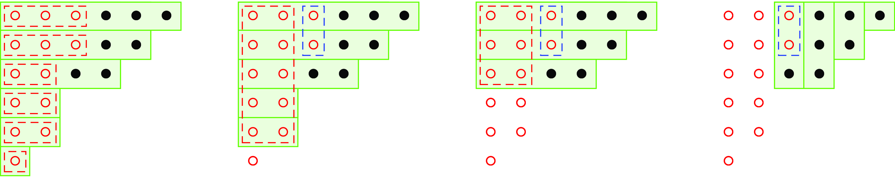
Now, if we draw Ferrers-type diagrams for the potential arguments $\underline{\mu}$ of $\lambda$ as sub-diagrams of Ferrers’ diagram of $\underline{\alpha}$ (representing $\mu_i$ by $\mu_i$ consecutive dots in row i) then $\lambda(\underline{\mu})$ is the number of dots in the sub-diagrams of $\underline{\mu}$ , while $\omega(\underline{\mu})$ gives a weighted count of those dots – a dot in the $j{\text{th}}$ column is counted with weight $p^{j-1}$ , as shown in Figure 1. Hence, to find the maximum of $\lambda$ , we need to maximize the number of dots in the sub-diagram corresponding to $\underline{\mu}$ , while keeping their total weight (total cost) $\omega(\underline{\mu})$ below ${D}/({p-1})$ . So, when selecting the dots in $\underline{\mu}$ , we just have to select the cheapest dots first. In our situation of column-wise increasing weights, we have to select the dots column by column, from left to right, starting with the left-most column with dots of lowest weight. Insight a column the order of selection does not matter, as long as the column is completely finished before we move to the next column. We may just go top-down inside columns, as in Figure 1. Following that order, we collect in step t a dot of weight $D_t$ , because that is how we defined $D_t$ . Hence, after t steps we obtain a $\underline{\mu}$ with

\[\omega(\underline{\mu})=D_1+ \cdots +D_t \quad \text{and} \quad \lambda(\underline{\mu})=t\,.\]

Our selection process has to stop when the limit ${D}/({p-1})$ for $\omega(\underline{\mu})$ is reached, that is when

\[t\,=\,t(D)\,{: \! =}\,\max\bigl\{0 \leq t \leq \alpha \mid D_1+ \cdots +D_{t} \leq \tfrac{D}{p-1}\bigr\}\,.\]

At that point, $\underline{\mu}=\underline{\mu}(D)$ is a maximum point of $\lambda$ , and the associated $\underline{n}(D)\,{: \! =}\,(p^{\mu_i}-1)_{i=1}^N$ is a minimum point of $\nu_p(\underline{\alpha},\bullet)$ in $\mathcal{D}(N,D)$ . The minimum value is

\[\mathcal{V}_p(\underline{\alpha},D)\,=\,\nu_p(\underline{\alpha},\underline{n}(D)) \,=\,\alpha-\lambda(\underline{\mu}) \,=\,\alpha-\max\bigl\{0 \leq t \leq \alpha \mid D_1+ \cdots +D_{t} \leq {D}/({p-1})\bigr\}\,.\]

Fig. 1.

The minimum weight of 9 dots inside $\underline{\alpha}=(6,5,3,1)$ is $D_1+D_2+ \cdots +D_9= 4+3p+2p^2$ .

Using our new formula, we can now show that $D\lt \sum_{i=1}^N(({p^{\alpha_i} \! -1})/({p-1}))$ is not just necessary for $\mathcal{V}_p(\underline{\alpha},D)\gt 0$ , as we already have seen in Proposition 3·4 (b), it is also sufficient:

Corollary 4·2. Maintain the setup of Theorem 4·1, we have

\[\mathcal{V}_p(\underline{\alpha},D)\gt 0 \quad \Longleftrightarrow \quad D\lt \sum_{i=1}^N\bigl(p^{\alpha_i} \! -1\bigr)\,.\]

Proof. With the last result in Example 6·3, we see that

\[D_1+ \cdots +D_{\alpha}\,=\,\alpha_1'p^0+ \cdots +\alpha_{N}'p^{N-1} \,=\,\sum_{i=1}^N\frac{p^{\alpha_i} \! -1}{p-1}\,.\]

So, by Theorem 4·1,

\begin{align*}\mathcal{V}_p(\underline{\alpha},D)\gt 0 \ \,&\Longleftrightarrow\ \, \max\bigl\{0 \leq t \leq \alpha \mid D_1+ \cdots +D_{t} \leq \tfrac{D}{p-1}\bigr\}\lt \alpha\\ \ \,&\Longleftrightarrow\ \, D_1+ \cdots +D_{\alpha}\nleq\tfrac{D}{p-1}\\ \ \,&\Longleftrightarrow\ \, D\lt \sum_{i=1}^N\bigl(p^{\alpha_i} \! -1\bigr)\,.\end{align*}

4·2. Alternative Expressions for $\mathcal{V}_p(\underline{\alpha},D)$ and Special Cases

In our main theorem (Theorem 1·6), we presented only one formula as the final result, as we did not want to make things any more complicated than necessary. That result can, however, be stated in different forms, by replacing the second lower bound

\[\alpha-\max\bigl\{0 \leq t \leq \alpha \mid D_1+ \cdots +D_{t} \leq \tfrac{D}{p-1}\bigr\} =\mathcal{V}_p(\underline{\alpha},D) \]

with an alternative expression for $\mathcal{V}_p(\underline{\alpha},D)$ . We present several alternative formulas in the second remark below (and in the subsequent corollary), after extracting an additional insights from our previous calculation of $\mathcal{V}_p(\underline{\alpha},D)$ in the following first remark:

Remark 4·3. In the proof of Theorem 4·1 we also constructed a minimum point $\underline{n}(D)$ of the function $\mathcal{D}(N,D){{\rightarrow}}\mathbb{N}\cup\{\infty\}$ , $\underline{n}\mapsto\nu_p(\underline{\alpha},\underline{n})$ . This point may be written as

\[\underline{n}(D)\,{: \! =}\, \bigl(p^{\mu_i(D)} \! -1\bigr)_{i=1}^N\,,\]

where

\begin{equation*} \mu_i(D)\,{: \! =}\,\begin{cases}Q(D)+1 & \text{if }1 \leq i \leq R(D) \\Q(D) & \text{if } R(D)\lt i \leq \alpha_{Q(D)+1}'\\\,\alpha_i & \text{if } \alpha_{Q(D)+1}' \! \lt i \leq N \end{cases}\end{equation*}

with

\begin{align*}Q(D)\,\,{: \! =}\,{}&\,\max\Bigl\{\textstyle0 \leq Q \leq \alpha_1\bigm{|}D_1+ \cdots +D_{\alpha_1'+ \cdots +\alpha_{Q}'} \leq \frac{D}{p-1}\Bigr\}\\={}&\,\max\Bigl\{\textstyle0 \leq Q \leq \alpha_1\bigm{|}\sum_{j=1}^{Q}\alpha_j'p^{j-1} \leq \frac{D}{p-1}\Bigr\}\end{align*}

and

\begin{align*}R(D)\,\,{: \! =}\,{}&\,\max\Bigl\{\textstyle0 \leq R \leq \alpha_{Q(D)+1}'\bigm{|}D_1+ \cdots +D_{\alpha_1'+ \cdots +\alpha_{Q(D)}'+R} \leq \frac{D}{p-1}\Bigr\}\\={}&\,\max\Bigl\{\textstyle0 \leq R \leq \alpha_{Q(D)+1}'\bigm{|}\sum_{j=1}^{Q(D)}\alpha_j'p^{j-1}+R\,p^{Q(D)} \leq \frac{D}{p-1}\Bigr\}.\end{align*}

Here, we regard sums of the form $\sum_{j=1}^{0}$ as zero and set $\alpha_{\alpha_1+1}'\,{: \! =}\,0$ , so that $\alpha_{Q(D)+1}'=0$ whenever $Q(D)=\alpha_1$ . Within a graphic representation as in Figure 1 or 2, the parameter $\mu_i(D)$ is the number of red dots in the $i^{\text{th}}$ row, Q(D) is the number of columns that are completely red, and R(D) is the number of red dots in the next column, if a next column exists. If there actually is a next column, after the last completely red one, this column is not completely red, i.e., $R(D)\lt \alpha_{Q(D)+1}'$ if (and only if) $Q(D)\lt \alpha_1$ .

Remark 4·4. Using the notations in Remark 4.3, the minimum value $\mathcal{V}_p(\underline{\alpha},D)$ can also be expressed in the following forms:

These four formulas can be derived from the formula $\mathcal{V}_p(\underline{\alpha},D)=\alpha-t(D)=\alpha-\lambda(\underline{\mu}(D))$ at the end of the proof of Theorem 4·1. The necessary simple rearrangements are illustrated in Ferrers diagrams in Figure 2. In each of the four cases, the minuends of the corresponding formula are shaded green, while the subtrahends are framed in red and blue. The difference $\mathcal{V}_p(\underline{\alpha},D)$ is represented by black dots. If $\underline{\alpha}=(6,5,4,2,2,1)$ and $t(D)=13$ (red dots), then, , , , and .

Fig. 2.

Four ways to calculate $\mathcal{V}_p(\underline{\alpha},D)$ (black dots) in Remark 4·4.

As in Corollary 1·8, our formula for $\mathcal{V}_p(\underline{\alpha},D)$ simplifies if $\alpha_1= \dots =\alpha_N$ . With the parameters

\[Q\,{: \! =}\,\bigl\lfloor\log_p(D/N+1)\bigr\rfloor \quad \ \text{and}\ \quad R\,{: \! =}\,\biggl\lfloor\frac{D-N(p^Q-1)}{(p-1)p^Q}\biggr\rfloor,\]

and with ${h}\,{: \! =}\,\max(h,0)$ for real numbers h, we obtain the following corollary:

Corollary 4·5. If $\alpha_1= \dots =\alpha_N$ then

\[\mathcal{V}_p(\underline{\alpha},D)\,=\, {N(\alpha_1-Q)-R}.\]

If $\alpha_1= \dots =\alpha_N=1$ then

\[\mathcal{V}_p(\underline{\alpha},D)\,=\,{N-\Bigl\lfloor\frac{D}{p-1}\Bigr\rfloor}.\]

Case 1: $D\lt N(p^{\alpha_1} \! -1)$ : In this case, it follows as in the proof of Corollary 1·8 in Section 3·5 that $Q(D)\lt \alpha_1$ and $R(D)\lt \alpha_{Q(D)+1}'$ . Hence,

\[Q(D)\,=\,\bigl\lfloor\log_p(D/N+1)\bigr\rfloor\,=:\,Q \quad \text{and} \quad R(D)\,=\,\biggl\lfloor\frac{D-N(p^Q-1)}{(p-1)p^Q}\biggr\rfloor\,=:\,R\,.\]

So, using the last formula of Remark 4·4 (to variate the approach in Section 3·5),

\[\mathcal{V}_p(\underline{\alpha},D)\,=\sum_{j=Q+1 \! \! }^{\alpha_1} \! \! \alpha_j'\,\,-R \,=\sum_{j=Q+1 \! \! }^{\alpha_1} \! \! N\,\,-R \,=\,N(\alpha_1-Q)-R \,=\,{N(\alpha_1-Q)-R}\,,\]

where the last equality follows from $N(\alpha_1-Q)-R=\mathcal{V}_p(\underline{\alpha},D) \geq 0$ .

In the subcase $\alpha_1= \dots =\alpha_N=1$ , this further simplifies to

\[\mathcal{V}_p(\underline{\alpha},D)\,=\,{N(1-0)-\Bigl\lfloor\frac{D-N(p^0-1)}{(p-1)p^0}\Bigr\rfloor}\,=\,{N-\Bigl\lfloor\frac{D}{p-1}\Bigr\rfloor}.\]

Case 2: $D \geq N(p^{\alpha_1} \! -1)$ : In this case, $Q \geq Q(D)=\alpha_1$ and thus ${N(\alpha_1-Q)-R}=0$ . By Corollary 4·2, this is the correct value for $\mathcal{V}_p(\underline{\alpha},D)$ if $D \geq N(p^{\alpha_1} \! -1)$ .

The formula for the subcase $\alpha_1= \dots =\alpha_N=1$ also gives the correct value 0.

5·1. A Preparatory Lemma

It turns out that the minimisation of $\mathcal N(\underline{n})$ leads to another optimisation problem that can be stated and solved in more general terms as follows:

Lemma 5·1. Assume $D\in\mathbb{N}$ , and let $\alpha,\Lambda_1,\Lambda_2, \dots ,\Lambda_\alpha,V_1,V_2, \dots\in\mathbb{Z}^+$ . Suppose that $(\Lambda_t)_{t=1}^{\alpha}$ is monotone increasing, that $(V_t)_{t\in\mathbb{Z}^+}$ is monotone decreasing, and that $\Lambda_1 \leq V_1$ . Also assume that $V_{t}=V_{1}$ for all $1 \leq t \leq s_0$ , where

\[s_0 \,{: \! =}\, {\bigl\lceil(\Lambda_1+ \cdots +\Lambda_{t_0}-D)/V_1\bigr\rceil} \,\ \text{with}\,\ t_0\,{: \! =}\,\max\{1 \leq t \leq \alpha \mid \Lambda_t \leq V_1\}\,.\]

Then the function $\mathbf{S}:\mathbb{N}\longrightarrow\mathbb{Z}$ given by

\[\mathbf{S}(s)\,{: \! =}\,s-\max\bigl\{0 \leq t \leq \alpha \mid \Lambda_1+ \cdots +\Lambda_{t} \leq V_1+V_2+ \cdots +V_s + D\bigr\}\]

has a minimum at the point $s_0$ , and

\[\mathbf{S}(s_0)\,=\,\begin{cases}s_0 - t_0 &\text{if $s_0\gt 0$,}\\- \max\bigl\{0 \leq t \leq \alpha \mid \Lambda_1+ \cdots +\Lambda_{t} \leq D\bigr\} &\text{if }s_0=0.\end{cases}\]

Proof. By definition, $s_0$ is the smallest element of $\mathbb{N}$ with

\[(\Lambda_1+ \cdots +\Lambda_{t_0}-D)/V_1 \leq s_0\,,\]

i.e., with

(5·1) \begin{equation}\Lambda_1+ \cdots +\Lambda_{t_0}\, \leq \,\,s_0V_1+D\,.\end{equation}

We calculate $\mathbf{S}(s_0)$ , $\mathbf{S}(s_0-s)$ and $\mathbf{S}(s_0+s)$ , for all permissible $s\in\mathbb{Z}^+ \! $ , to show that $\mathbf{S}(s_0)$ is a minimum of $\mathbf{S}$ . For this purpose it is convenient to extend the sequence $(\Lambda_t)_{t=1}^{\alpha}$ to an infinite sequence by setting $\Lambda_{\alpha+1},\Lambda_{\alpha+2}, \dots\,{: \! =}\,\infty$ . With that extension $t_0=\max\{t\in\mathbb{Z}^+ \! \mid \Lambda_t \leq V_1\}$ .

Case 1: $s_0\gt 0$ : In this case, by (5·1),

(5·2) \begin{align}\Lambda_1+ \cdots +\Lambda_{t_0}&\, \leq \,V_1+ \cdots +V_{s_0}+D\end{align}

but, by the minimality of $s_0$ in (5·1), also

(5·3) \begin{align}\Lambda_1+ \cdots +\Lambda_{t_0} &\,\gt \,V_1+ \cdots +V_{s_0-1}+D\,. \end{align}

In the last inequality, if $s_0 \geq 2$ , each summand $V_j$ on the right is at least as large as each of the summands $\Lambda_i$ on the left, because $\Lambda_1 \leq \dots \leq \Lambda_{t_0} \leq V_1= \dots =V_{s_0-1}$ . Therefore, we can remove an equal number of those summands on both sides without destroying the inequality. Also, the bigger left sum must contain more of the smaller $\Lambda $ -summands than the smaller right sum contains of the bigger $V$ -summands, because $D \geq 0$ . In particular, for each $0\lt s \leq s_0$ ,

(5·4) \begin{equation}\Lambda_1+ \cdots +\Lambda_{t_0-s+1}\,\gt \,V_1+ \cdots +V_{s_0-s}+D\,.\end{equation}

But, also $ \dots \geq \Lambda_{t_0+2} \geq \Lambda_{t_0+1}\gt V_1= V_{s_0} \geq V_{s_0+1} \geq \dots $ . So, we can also add an equal number of subsequent summands on both sides of (5·3). For each $s\in\mathbb{N}$ ,

(5·5) \begin{equation}\Lambda_1+ \cdots +\Lambda_{t_0+s+1}\,\gt \,V_1+ \cdots +V_{s_0+s}+D\,.\end{equation}

Based on these inequalities, we can now calculate $\mathbf{S}(s_0)$ , $\mathbf{S}(s_0-s)$ and $\mathbf{S}(s_0+s)$ . It follows from (5·3) and (5·5) with $s=0$ that

\[\mathbf{S}(s_0)\,=\,s_0 - t_0\,.\]

It follows from (5·4) that, for each $0\lt s \leq s_0$ ,

\begin{align*}\mathbf{S}(s_0-s)\, \geq \,s_0 - s - (t_0-s)\,=\,s_0 - t_0\,=\,\mathbf{S}(s_0)\,.\end{align*}

And, it follows from (5·5) that, for each $s\in\mathbb{N}$ ,

\[\mathbf{S}(s_0+s)\, \geq \,s_0 + s - (t_0+s)\,=\,\mathbf{S}(s_0)\,.\]

We see that $\mathbf{S}$ attains a minimum at $s_0$ and $\mathbf{S}(s_0)=s_0-t_0$ .

Case 2: $s_0=0$ : In this case, if we set

\[t(D)\,{: \! =}\,\max\bigl\{0 \leq t \leq \alpha \mid \Lambda_1+ \cdots +\Lambda_{t} \leq D\bigr\} =\max\bigl\{t\in\mathbb{N} \mid \Lambda_1+ \cdots +\Lambda_{t} \leq D\bigr\}\,,\]

by the maximality of t(D),

(5·6) \begin{equation}\Lambda_1+ \cdots +\Lambda_{t(D)+1}\,\gt \,D\,.\end{equation}

Moreover, $ \dots \geq \Lambda_{t(D)+2} \geq \Lambda_{t(D)+1} \geq \Lambda_{t_0+1}\gt V_1 \geq V_2 \geq \dots $ since $t(D) \geq t_0$ , by (5·1). Hence, we can add summands to (5·6), in the same way as we did it to get (5·5) from (5·3). For each $s\in\mathbb{N}$ ,

\[\Lambda_1+ \cdots +\Lambda_{t(D)+s+1}\,\gt \,V_1+ \cdots +V_{s}+D\,,\]

and thus

\[\mathbf{S}(s)\, \geq \,s - (t(D)+s)\,=\,0 - t(D)\,=\,\mathbf{S}(0)\,.\]

So, $\mathbf{S}$ attains a minimum at 0 and $\mathbf{S}(0)= -\max\bigl\{0 \leq t \leq \alpha \mid \Lambda_1+ \cdots +\Lambda_{t} \leq D\bigr\}$ .

5·2. The Minimum Value of $\mathcal N$ over $[\hat{\underline{n}}(\beta)]$

We are ready to determine the minimum value of $\mathcal N(\underline{n})$ when $\underline{n}$ is ranging over $[\hat{\underline{n}}(\beta)]$ :

Lemma 5·2. In the settings described at the beginning of Section 5, with the derived values $\breve\alpha_1, \dots,\breve\alpha_N,\breve\alpha,\breve{\mathcal{A}},\mathcal B$ as in Theorem 1·6, and for every integer

\[\beta\,\gt \,s_0\,{: \! =}\,{\biggl\lceil\frac{\breve{\mathcal{A}}-\mathcal B}{d_1p^{{\beta_1-1}}}\biggr\rceil}\,,\]

we have

\[\min_{\underline{n}\in[\hat{\underline{n}}(\beta)]}\mathcal N(\underline{n})\,=\,\begin{cases}s_0+\alpha-\breve\alpha&\text{if } \breve{\mathcal{A}}\gt \mathcal B,\\\alpha-\max\bigl\{1 \leq t \leq \alpha \mid D_1+ \cdots +D_{t} \leq \mathcal B\bigr\}&\text{if } \breve{\mathcal{A}} \leq \mathcal B.\end{cases}\]

Step 1. If $n_1 \leq p^{\beta_1} \! -1$ then ${\Bigl\lceil{(n_1-(p^{\beta_1} \! -1))}/({(p-1)p^{\beta_1-1}})\Bigr\rceil}=0$ . So, as $\mathcal V_p(\underline{\alpha},\bullet)$ is monotone decreasing,

\[n_1 \leq p^{\beta_1} \! -1\ \ \Longrightarrow\ \ \mathcal N(n_1,n_2, \dots,n_r) \geq \mathcal N(p^{\beta_1} \! -1,n_2, \dots,n_r).\]

This shows that, in order to find a minimum, we may replace values of $n_1$ below $p^{\beta_1} \! -1$ with $p^{\beta_1} \! -1\in[\hat n_1(\beta)]$ . More generally, for each $1\le j \leq r$ , we may assume $n_j \geq p^{\beta_j} \! -1$ . In other words, we may write each $n_j$ as $u_j+p^{\beta_j} \! -1$ with $u_j \geq 0$ , which leads to the simplifications

\[{\biggl\lceil\frac{n_j-(p^{\beta_j} \! -1)}{(p-1)p^{\beta_j-1}}\biggr\rceil}\,=\, {\biggl\lceil\frac{u_j}{(p-1)p^{\beta_j-1}}\biggr\rceil}\,=\, \biggl\lceil\frac{u_j}{(p-1)p^{\beta_j-1}}\biggr\rceil\]

and

\[\mathcal{V}_p\Bigl(\underline{\alpha}\,,\,{\textstyle\sum_{j=1}^r}d_jn_j\Bigr)\,=\,\mathcal{V}_p\Bigl(\underline{\alpha}\,,\,{\textstyle\sum_{j=1}^r}d_ju_j+ (p-1)\mathcal B\Bigr)\,.\]

So, with

\[\mathcal U(\underline{u}) \,{: \! =}\,\sum_{j=1}^r\biggl\lceil\frac{u_j}{(p-1)p^{\beta_j-1}}\biggr\rceil + \mathcal{V}_p \Bigl(\underline{\alpha}\,,\,{\textstyle\sum_{j=1}^r}d_ju_j + (p-1)\mathcal B\Bigr)\]

we have $\mathcal N(\underline{n})=\mathcal U(\underline{u})$ , and thus

\[\min_{\underline{n}\in[\hat{\underline{n}}(\beta)]}\mathcal N(\underline{n}) \,=\, \min_{\underline{u}\in[\underline{\hat u}(\beta)]}\mathcal U(\underline{u})\,.\]

with updated ranges

\[\hat u_j(\beta)\,{: \! =}\,\hat n_j(\beta)-(p^{\beta_j} \! -1)\,=\,(\beta-1)p^{\beta_j-1}(p-1)\,.\]

Step 2. To find a minimum of $\mathcal U$ over $[\underline{\hat{u}}(\beta)]=\prod_{j=1}^r[\hat u_j(\beta)]$ , we can replace the domain $[\hat{u}_j(\beta)]=\{0,1, \dots,\hat u_j(\beta)\}$ of each $u_j$ with the smaller domain

\begin{align*} [\hat u_j(\beta)]\cap p^{\beta_j -1}(p-1)\mathbb{Z} &\,=\,\{0, p^{\beta_j-1}(p-1), \dots, (\beta-1)p^{\beta_j-1}(p-1)\}\\ &\,=\,p^{\beta_j-1}(p-1)[\beta-1]\,.\end{align*}

Indeed, if the $j{\text{th}}$ argument $u_j\in[\hat u_j]$ of $\mathcal U(u_1, \dots,u_r)$ is replaced with the first multiple of $p^{\beta_j-1}(p-1)$ above or equal to $u_j$ (which still lies inside $[\hat u_j(\beta)] = [(\beta-1)p^{\beta_j-1}(p-1)]$ ), then the summand $\Bigl\lceil{u_j}/({p^{\beta_j-1}(p-1)})\Bigr\rceil$ of $\mathcal U(\underline{u})$ stays the same and $\mathcal U(\underline{u})$ certainly does not increase. The minimum of $\mathcal U$ is already attained at a point $\underline{u}$ of the smaller domain $\prod_{j=1}^r\bigl(p^{\beta_j-1} (p-1)[\beta-1]\bigr)\subseteq[\underline{\hat u}(\beta)]$ . Hence, with

\begin{align*}\mathcal T(t_1, \dots,t_r)\ \,{: \! =}\,{}&\ \ \mathcal U\bigl(p^{\beta_1-1}(p-1)t_1, \dots,p^{\beta_r-1}(p-1)t_r\bigr)\\={}&\ \ t_1 + \cdots + t_r+ \mathcal{V}_p\Bigl(\underline{\alpha}\,,\,{\textstyle\sum_{j=1}^r}d_jp^{\beta_j-1}(p-1)t_j+ (p-1)\mathcal B\Bigr)\end{align*}

we have

\[\min_{\underline{n}\in[\hat{\underline{n}}]}\mathcal N(\underline{n}) \,=\,\min_{\underline{u}\in[\underline{\hat u}]}\mathcal U(\underline{u}) \,=\,\min_{\underline{t}\in[\beta-1]^r}\mathcal T(\underline{t})\,.\]

Step 3. In our search for the minimum value that $\mathcal{T}(t_1, \dots,t_r)$ may take, we can now modify any two arguments $t_i$ and $t_j$ with $i\lt j$ by replacing $t_j$ with $t_j-1$ and $t_i$ with $t_i+1$ . If we view the term $d_jp^{\beta_j-1}(p-1)t_j$ as sum of $t_j$ equal summands $d_jp^{\beta_j-1}(p-1)$ , this step changes one of the $t_j$ summands $d_jp^{\beta_j-1}(p-1)$ inside the argument of $\mathcal V_p(\underline{\alpha},\bullet)$ into one additional summand $d_ip^{\beta_i-1}(p-1)$ , of which we then have $t_i+1$ . Since

\[d_1p^{\beta_1-1} \geq d_2p^{\beta_2-1} \geq \dots \geq d_rp^{\beta_r-1} \]

and $\mathcal V_p(\underline{\alpha},\bullet)$ is monotone decreasing, we have

\[\mathcal T( \dots,t_i+1, \dots,t_j-1, \dots \! ) \, \leq \,\mathcal T( \dots,t_i, \dots,t_j, \dots \! )\,.\]

The only restriction to such modifications is that all argument $t_j$ must stay within their domains $[\beta-1]$ . They cannot increase above $\beta-1$ or go below 0. Through repeated applications of our modification, we can empty some $t_j$ and fill others. This shows that the minimum is attained at a point of the form

\[(t_1,t_2, \dots,t_r)\,=\,(\beta-1,\beta-1, \dots,\beta-1,x,0,0, \dots,0)\,.\]

At such points, we have

\[\mathcal T(t_1,t_2, \dots, t_r)\,=\,s + \mathcal{V}_p\Bigl(\underline{\alpha}\,,\,(p-1)(V_1+V_2+ \cdots +V_s + \mathcal B)\Bigr)\,,\]

where $s=t_1+t_2+ \cdots +t_r=\beta-1+\beta-1+ \cdots +\beta-1+x \leq r(\beta-1)$ , and where

\[\bigl(V_1,V_2, \dots,V_{r(\beta-1)}\bigr)\,{: \! =}\,\bigl(\,\underbrace{d_1p^{\beta_1-1} \! , \dots,d_1p^{\beta_1-1}}_{\beta-1\ \text{times} \! },\, \dots, \,\underbrace{d_rp^{\beta_r-1} \! , \dots,d_rp^{\beta_r-1}}_{\beta-1\ \text{times}}\,\bigr)\,.\]

Hence, with the function

\[\mathcal S:[r(\beta-1)]{{\rightarrow}}\mathbb{N}\,, \quad \mathcal S(s)\,{: \! =}\,s + \mathcal{V}_p\Bigl(\underline{\alpha}\,,\,(p-1)(V_1+V_2+ \cdots +V_s + \mathcal B)\Bigr)\,,\]

we have

\[\min_{\underline{n}\in[\hat{\underline{n}}(\beta)]}\mathcal N(\underline{n}) \,\,=\min_{\underline{t}\in[\beta-1]^r}\mathcal T(\underline{t}) \,\,=\min_{s\in[r(\beta-1)]}\mathcal S(s)\,.\]

Step 4. To find the minimum of $\mathcal S$ , we use Lemma 5·1 with $D\,{: \! =}\,\mathcal B$ , $\alpha\,{: \! =}\,\alpha_1+ \cdots +\alpha_N$ , and $\Lambda_t\,{: \! =}\,D_t$ for all $1 \leq t \leq \alpha$ . We also use the values $V_t$ as defined above for all $1 \leq t \leq r(\beta-1)$ , and set $V_t\,{: \! =}\,V_{r(\beta-1)}$ for all $t\gt r(\beta-1)$ . With the infinite sequence $(V_t)_{t\in\mathbb{Z}^+}$ the domain of $\mathcal S$ can be extended to $\mathbb{N}$ (with the hope not to alter its minimum in doing so), as the expression

\begin{align*}\mathcal{V}_p\Bigl(\underline{\alpha}\,,\,&(p-1)(V_1+ \cdots +V_s + \mathcal B)\Bigr)\\ &=\,\alpha-\max\bigl\{0 \leq t \leq \alpha \mid \Lambda_1+ \cdots +\Lambda_{t} \leq V_1+ \cdots +V_s + \mathcal B\bigr\}\end{align*}

makes sense for all $s\in\mathbb{N}$ . The extended function $\mathcal S:\mathbb{N}{{\rightarrow}}\mathbb{N}$ is then almost the same as the function $\mathbf{S}:\mathbb{N}{{\rightarrow}}\mathbb{Z}$ in Lemma 5·1. For all $s\in\mathbb{N}$ ,

\[\mathcal S(s)\,{: \! =}\,\mathbf{S}(s) + \alpha\,.\]

We also have $\Lambda_1 \leq V_1$ as required in Lemma 5·1. Moreover, as in our situation the sequence $(\Lambda_t)$ contains repetitions of lengths $\alpha_1',\alpha_2', \dots,\alpha'_{\alpha_1}$ , the parameter

\[t_0\,{: \! =}\,\max\bigl\{1 \leq t \leq \alpha \mid \Lambda_t \leq V_1\bigr\}\]

in Lemma 5·1 can be written as

\[t_0\,=\,\alpha_1'+ \cdots +\alpha_{i_0}' \quad \text{with} \quad i_0\,{: \! =}\,\max\bigl\{1 \leq i \leq \alpha_1 \mid p^{i-1} \leq d_1p^{\beta_1-1}\bigr\}\,.\]

Here, the inequality $p^{i-1} \leq d_1p^{\beta_1-1}$ can be written as $i \leq \beta_1+\log_p\bigl(d_1\bigr)$ , and the biggest integer i with this property is $\beta_1+\lfloor\log_p\bigl(d_1\bigr)\rfloor$ . But, in the definition of $i_0$ we also have the requirement $i \leq \alpha_1$ , so that

\[i_0\,=\,\max\bigl\{1 \leq i \leq \alpha_1 \mid p^{i-1} \leq d_1p^{\beta_1-1}\bigr\} \,=\,\min\bigl(\alpha_1,\beta_1+\lfloor\log_p\bigl(d_1\bigr)\rfloor\bigr) \,=\,\breve\alpha_1\,.\]

With that and the second equation of Example 6·4 we get

\[t_0\,=\,\alpha_1'+ \cdots +\alpha_{i_0}'\,=\,\alpha_1'+ \cdots +\alpha_{\breve\alpha_1}'\,=\,\breve\alpha_1+ \cdots +\breve\alpha_N \,=\,\breve\alpha\,.\]

With the third equation of Example 6·4, we further see that

\[\Lambda_1+ \cdots +\Lambda_{t_0} \,=\,\Lambda_1+ \cdots +\Lambda_{\breve\alpha} \,=\,\alpha_1'p^0+ \cdots +\alpha_{\breve\alpha_1}'p^{\breve\alpha_1-1} \,=\,\sum_{i=1}^N\frac{p^{\breve\alpha_i} \! -1}{p-1} \,=:\,\breve{\mathcal{A}}\,.\]

In particular, the definition of $s_0$ in Lemma 5·1 coincides with the current one:

\[s_0 \,=\,{\bigl\lceil(\Lambda_1+ \cdots +\Lambda_{t_0}-\mathcal B)/V_1\bigr\rceil} \,=\,{\biggl\lceil\frac{\breve{\mathcal{A}} -\mathcal B}{d_1p^{{\beta_1-1}}}\biggr\rceil}\,.\]

As assumed, this number is smaller than $\beta$ , i.e., $s_0 \leq \beta-1$ . This shows that $V_{t}=V_{1}$ for all $1 \leq t \leq s_0$ , as required in Lemma 5·1. But, $s_0 \leq \beta-1$ also shows that the minimum point $s_0$ of $\mathbf{S}$ lies inside $[r(\beta-1)]$ . Hence, the minimum point $s_0$ of $\mathbf{S}$ is also a minimum point of $\mathbf{S}|_{[r(\beta-1)]}$ and of $\mathcal S|_{[r(\beta-1)]}$ . Thus, Lemma 5·1 yields

\begin{align*}\min_{\underline{n}\in[\hat{\underline{n}}(\beta)]}\mathcal N(\underline{n}) &\,=\,\min_{s\in[r(\beta-1)]}\mathcal S(s)\\ &\,=\,\,\,\mathbf{S}(s_0)\,+\,\alpha\\ &\,=\,\begin{cases}s_0+\alpha-\breve\alpha&\text{if } \breve{\mathcal{A}}\gt \mathcal B,\\\alpha-\max\bigl\{1 \leq t \leq \alpha \mid D_1+ \cdots +D_{t} \leq \mathcal B\bigr\}&\text{if } \breve{\mathcal{A}} \leq \mathcal B.\end{cases}\end{align*}

6·1. Two General Conjugation Lemmas

Our first lemma, while certainly not a new deep insight, is formulated in a way that is helpful for our calculations.

Lemma 6·1. Let $(a_i)\in(\mathbb{Z}^+)^N$ be monotone decreasing, and $1 \leq m \leq a_1$ . We have the following identity in $\mathbb{Z}[x]$ :

\[a_{m}'x^{m}+a_{m+1}'x^{m+1}+ \cdots +a_{a_1}'x^{a_1} \,=\,\sum_{i=1}^{a_{m}'}\bigl(x^{m}+x^{m+1}+ \cdots +x^{a_i}\bigr)\,.\]

Proof. Both polynomials have degree at most $a_1$ , and there are no monomials of degree less than m. For each $m \leq j \leq a_1$ , however, the coefficient of $x^j$ in the standard expansion of the right polynomial is

\[\# \bigl\{1 \leq i \leq a_{m}' \mid a_i \geq j\bigr\} \,=\,\# \bigl\{1 \leq i \leq N \mid a_i \geq j\bigr\}\,=\,a_j'\,,\]

because

\[a_{i} \geq j \quad \Longrightarrow \quad a_{i} \geq m \quad \Longrightarrow \quad a_{1}, \dots,a_{i} \geq m \quad \Longrightarrow \quad i \leq a_{m}'\,,\]

i.e., it is the same as the coefficient of $x^j$ in the left polynomial.

The next lemma is obvious if we consider the minimum as given by the intersection of two Ferrers diagrams, because “intersecting” and “reflecting” commute.

Lemma 6·2. If the two sequences $(a_i),(b_i)\in(\mathbb{Z}^+)^N$ are monotone decreasing, then the sequence $(c_i)\,{: \! =}\,\bigl(\min(a_i,b_i)\bigr)\in(\mathbb{Z}^+)^N$ is also monotone decreasing. The conjugate sequences $(a_j')$ , $(b_j')$ , and $(c_j')$ have lengths $a_1$ , $b_1$ , and $c_1=\min(a_1,b_1)$ , respectively; and for all $1 \leq j \leq c_1$ ,

\[c_j'\,=\,\min(a_j',b_j')\,.\]

6·2. Special Cases

Example 6·3. If $x=1$ in Lemma 6·1, we obtain, for all $1 \leq m \leq a_1$ ,

\[\sum_{j=m}^{a_1} \! a_j'\,=\,\sum_{i=1}^{a_{m}'}\bigl(a_i-m+1\bigr)\,.\]

If $m=1$ then $a_m'=a_1'=N$ , and then $x=1$ leads to

\[a_1'+ \cdots +a_{a_1}'\,=\,a_1+ \cdots +a_{N}\,.\]

If $m=1$ and $x=p$ , then Lemma 6·1 yields

\[a_1'p^0+ \cdots +a_{a_1}'p^{a_1-1}\,=\,\sum_{i=1}^{N}\bigl(p^{0}+p^{1}+ \cdots +p^{a_i-1}\bigr) \,=\,\sum_{i=1}^N\frac{p^{a_i} \! -1}{p-1}\,.\]

Example 6·4. If the sequence $(b_i)$ in Lemma 6·2 is constant equal to a number $b\in\mathbb{Z}^+$ , we obtain as the conjugate of the sequence $(c_i)\,{: \! =}\,\bigl(\min(a_i,b)\bigr)\in(\mathbb{Z}^+)^N$ the sequence

\[(c_1',c_2', \dots,c_{c_1}')\,=\,(a_1',a_2', \dots,a_{c_1}')\,.\]

So, if we apply Lemma 6·1 to $(c_i)$ with $m=1$ and $x=1$ , we get

\[a_1'+ \cdots +a_{c_1}'\,=\,c_1+ \cdots +c_{N}\,.\]

If instead $m=1$ and $x=p$ , we get

\[a_1'p^0+ \cdots +a_{c_1}'p^{c_1-1}\,=\,\sum_{i=1}^{N}\bigl(p^{0}+p^{1}+ \cdots +p^{c_i-1}\bigr)\,=\,\sum_{i=1}^N\frac{p^{c_i} \! -1}{p-1}\,.\]