2.1. General presentation

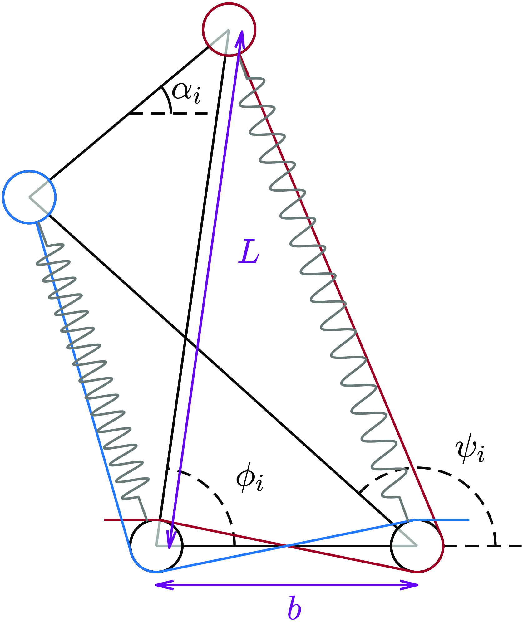
The robots under study are built with a series of X-joints (Figure 1). The robot configuration $\boldsymbol{\alpha }$ is defined by the angle $\alpha _i$ between the base bar and the top bar of each X-joint. Each X-joint is actuated by two antagonistic cables, which are pulled by motors on either side of the joint (Figure 1). This actuation scheme allows motion in any direction starting from the equilibrium configuration at rest, that is, where there is no tension in the cable. Additionally, each joint is equipped with a spring in parallel with the cable. This spring serves to stabilize the robot equilibrium configuration at rest.

When each X-joint is actuated by a set of two cables that differs from the set of cables used in other X-joints, each X-joint can be actuated independently, resulting in a fully actuated robot. For a fully actuated robot with $N_j$ joints, the number of cables, denoted as $N_c$ , can vary from $N_j+1$ to $2N_j$ . In the work presented in ref. [Reference Fasquelle, Khanna, Chevallereau, Chablat, Creusot, Jolivet, Lemoine and Wenger2], the control of a fully actuated robot with $N_J=3$ joints and $N_c=4$ cables was demonstrated.

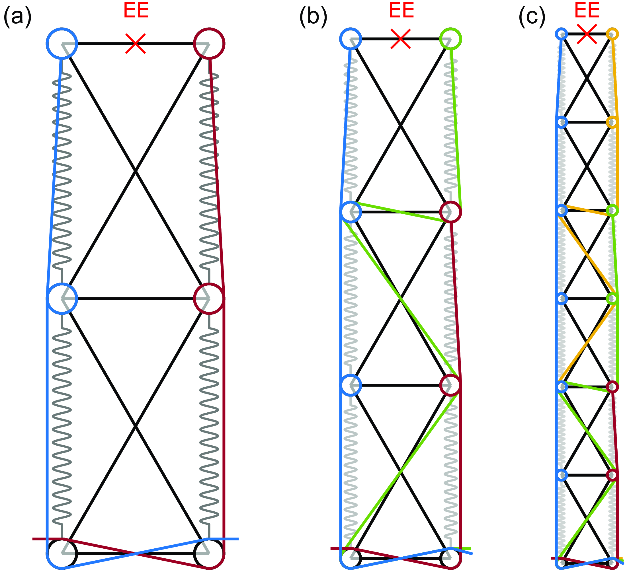
In this paper, the robots studied are in fact underactuated. For the 3 robots shown in Figure 2, indeed, $N_c \leq N_j$ . The aim of this paper is to control such robots.

The first robot under consideration is the simplest underactuated model, comprised of two joints actuated by two cables (see Figure 2 a). These two cables are attached to both joints and exert actions on the two joints that are therefore dependant. Thus, only one variable can be controlled. This simple underactuated manipulator is studied for the purpose of better illustrating the difficulties encountered. Given the aim of controlling the end effector (EE) motion, one can consider controlling the position coordinates $x$ or $y$ or the orientation angle $\gamma$ of the EE. Since only one output can be controlled for this simple robot and there are two cables, the cable forces are chosen to maintain positive cable tensions. It is possible to adjust stiffness but we prefer to minimize the forces while ensuring that cable tensions remain positive.

Figure 1.

A X-joint, $L$ is the length of the diagonal bars and $b$ is the length of the base and top bars. $\alpha _i$ is the angle between the top bar and the base bar, and $\phi _i$ and $\psi _i$ are the angles between the diagonal bars and the base bar.

Figure 2.

The three underactuated robots under study. (a) Has 2 joints and 2 cables, (b) has 3 joints and 3 cables, and (c) has 6 joints and 4 cables.

The second robot studied consists of three joints actuated by three cables. One cable runs along the left side of each joint, and two cables are routed along the right side as shown in Figure 2 b. In this robot, two groups of joints share the same set of cables. The first group comprises the first two joints, which are actuated by the blue and red cables. The second group corresponds to the third joint, which is actuated by the blue and green cable. A group of joints that share the same set of cables will be referred to as metamodule in the following. Accordingly, the second robot has 2 metamodules and two variables can be thus controlled, which we choose as the two position coordinates $x$ and $y$ of the EE. This robot will be investigated both theoretically and experimentally.

The third robot studied consists of six joints actuated by four cables, one on the left and the other three on the right (see Figure 2 c). These four cables enable the control of all EE coordinates $x$ , $y$ , and $\gamma$ . This robot has 3 metamodules defined by joints 1 and 2, joints 3 and 4, and joints 5 and 6, respectively. This robot represents a practical example of a planar manipulator suitable for real-world applications.

For the second and third robot, a single cable is responsible for pulling all joints on one side, while the other cables act on different groups of joints on the opposite side. This choice draws inspiration from the long ventral muscle that connects all vertebrae in various bird species [Reference Terray, Plateau, Abourachid, Böhmer, Delapré, la Bernardie and Cornette33].

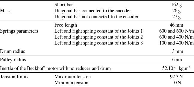
The routing of the cables is implemented with pulleys equipped with ball bearings, which ensure that there is no friction between the cables and the bars. The X-joint dimensions are $L$ = 0.1 m and $b$ =0.05 m, and the mass of a short (resp. diagonal) bar is 162 g (resp. 26 g). The short bar is heavier because, on our prototype, it is actually composed of two bars in parallel linked by two shafts on which the pulleys are fixed. Moreover, the encoder is also fixed on one of these two bars. We assume that the orientation angle $\alpha _i$ of each joint is bounded by $-90^\circ$ and $90^\circ$ .

2.2. Dynamic modeling

The dynamic model can be computed using the Lagrange formalism. The equation linking joint accelerations $\ddot{\boldsymbol{\alpha}}$ to cable tensions $\boldsymbol{f}$ can be written as [Reference Fasquelle, Furet, Chevallereau and Wenger14]

(1) \begin{equation} \mathbf{M}_\alpha (\boldsymbol{\alpha })\ddot{\boldsymbol{\alpha}}+\mathbf{d}_c(\boldsymbol{\alpha },\dot{\boldsymbol{\alpha}})=\mathbf{Z}(\boldsymbol{\alpha })\,\boldsymbol{f} \end{equation}

where:

• • $\mathbf{M}_\alpha (\boldsymbol{\alpha })$ is the robot inertia matrix,

• • $\mathbf{d}_c(\boldsymbol{\alpha },\dot{\boldsymbol{\alpha}})$ contains the gravitational effect, the springs effect, the centrifugal and coriolis effect, and the friction. For this study, the friction model employed is viscous friction in the joint, defined as $\boldsymbol{f}_r(\boldsymbol{\alpha },\dot{\boldsymbol{\alpha}})=-f_v\left (2\left (\frac{\partial \boldsymbol{\phi }}{\partial \boldsymbol{\alpha }}\right )^2+2\left (\frac{\partial \boldsymbol{\psi }}{\partial \boldsymbol{\alpha }}\right )^2\right )\dot{\boldsymbol{\alpha}}$ where $f_v$ is a constant. This corresponds to viscous friction at passive joints between the bars of the X-joints.

• • $\mathbf{Z}(\boldsymbol{\alpha })$ is the matrix that relates cable tensions to the torques they produce around the joint.

The $\mathbf{Z}(\boldsymbol{\alpha })$ matrix is of size $N_j \times N_c$ . This matrix plays a significant role in understanding how actuation influences the different joints, making it essential in the study of underactuation. We provide below a concise overview for quick comprehension, more details can be found in ref. [Reference Fasquelle, Khanna, Chevallereau, Chablat, Creusot, Jolivet, Lemoine and Wenger2]. Each term of $\mathbf{Z}(\boldsymbol{\alpha })$ is expressed by $Z(\alpha )(i, j)=-\frac{\partial l_j(\alpha _i)}{\partial \alpha _i}$ , where $l_j$ is the length of cable $j$ . If cable $j$ runs along the left (resp. right) side of joint $i$ , the term $Z(i, j)$ is positive (resp. negative). If cable $j$ does not pass through joint $i$ , the $Z(i, j)$ term is zero. When cable $j$ crosses joint $i$ along a diagonal bar, the $Z(i, j)$ term is proportional to the size of the pulleys and is relatively small compared to the case where the cable passes laterally. For joints within the same group, that is, those operated by the same set of cables, the same line will appear in the $Z$ matrix if the joint angles are identical and if the pulleys radius is neglected.

In the case of fully actuated robots, there are more cables than joints (at a minimum of $N_c=N_j+1$ ) and $rank(\mathbf{Z}(\boldsymbol{\alpha }))=N_j$ . In underactuated robots with a single cable controlling all the joints on one side, there are more (or the same number of) joints than cables, which typically results in $rank(\mathbf{Z}(\boldsymbol{\alpha }))=N_c$ .

2.3. Inverse kineto-static model

Our control objective is to achieve desired motions for $N_c-1$ EE coordinates grouped within a vector denoted as the controlled variables $\boldsymbol{q}$ . The studied motions is such that the robot starts and stops in an equilibrium configuration. Note that the 3 robots studied are underactuated. This section aims to explore the joint equilibrium configurations $\boldsymbol{\alpha }$ corresponding to a desired EE pose denoted as $\boldsymbol{q}^{\boldsymbol{d}}$ .

We examine a 6-joint robot equipped with 4 cables, as illustrated in Figure 2 c. Gravity is considered, and the base is oriented at $\frac{\pi }{4}$ . Symmetrical springs are connected on both sides of the joints, with spring constants equal to 1000, 850, 800, 650, 400, and 250 N/m, from the base joint to the last joint. The pulleys have a radius of 0.005 m. Our control objective is to control the EE position and orientation: $\boldsymbol{q}=[x, y, \gamma ]^\top$ , which can be expressed as a function $\mathbf{f}_q$ depending on the joint angles $\boldsymbol{\alpha }$ . Given a specified desired pose $\boldsymbol{q}^d$ , we determine the equilibrium configuration $\boldsymbol{\alpha }$ that minimizes cable tensions:

(2) \begin{align} (\boldsymbol{\alpha },\boldsymbol{f})&=\min _{\boldsymbol{\alpha },\boldsymbol{f}}||\boldsymbol{f}||\nonumber \\ &s.t.\;\left \{\begin{array}{l} \boldsymbol{d}_c(\boldsymbol{\alpha },0)=\mathbf{Z}(\boldsymbol{\alpha })\,\boldsymbol{f}\\ \boldsymbol{f}_q(\boldsymbol{\alpha })=\boldsymbol{q}^d\\ min(\boldsymbol{f}) \ge f_{min}\\ \end{array} \right . \end{align}

where $\boldsymbol{d}_c(\boldsymbol{\alpha },0)=\mathbf{Z}(\boldsymbol{\alpha })\,\boldsymbol{f}$ is the static model derived from Eq. (1) and $f_{min}$ is the minimum tension that we want to apply in the cables.

Figure 3.

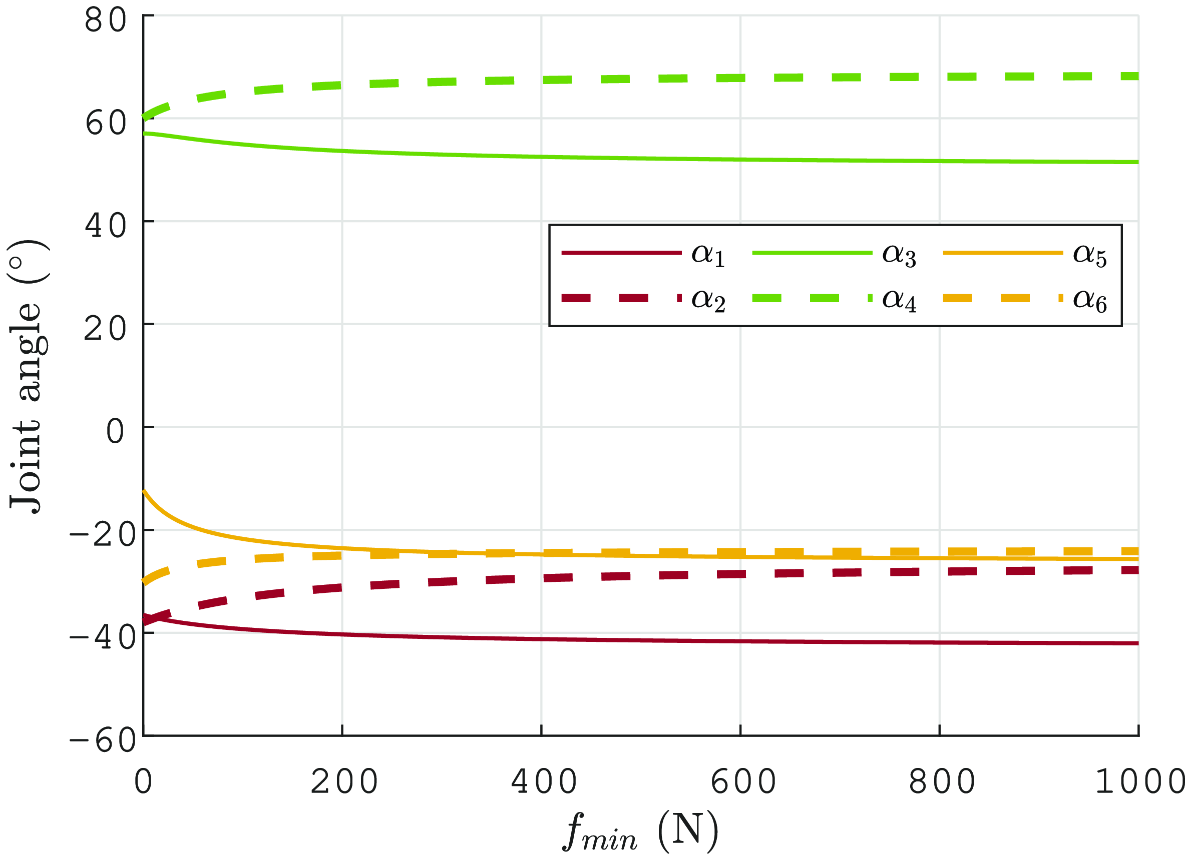
Joint angle evolution as a function of the lowest cable tension $f_{min}$ for $[x,y]=[{-}0.26,0.36]^\top$ m and $\gamma =\frac{\pi }{4}$ rad. The angles represented with the same color belong to the same metamodule. Continuous lines correspond to the first joint of the metamodule, while dashed lines represent the second joint of the metamodule.

Figure 4.

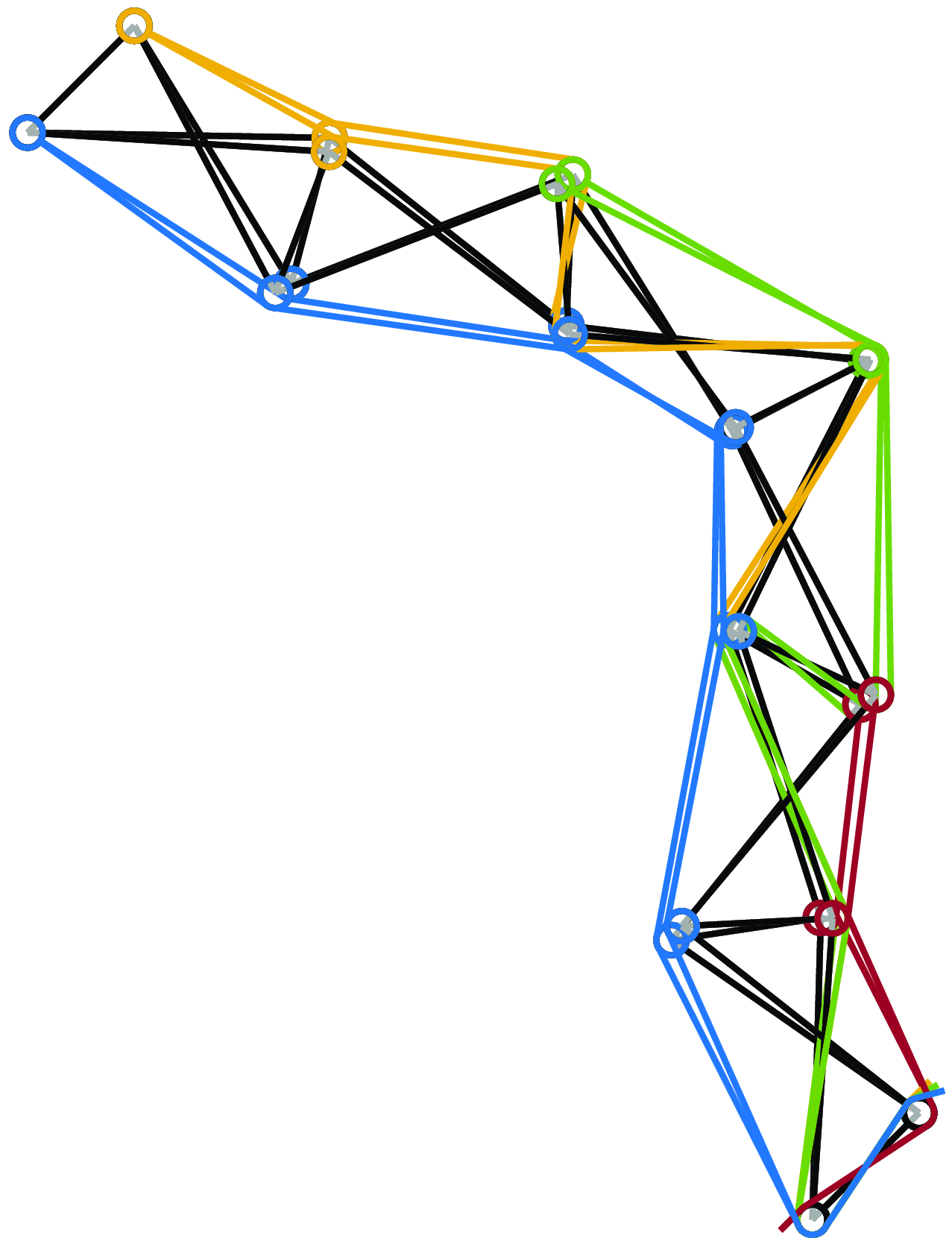
Robot configuration at $f_{min}=0$ n and $f_{min}=1000$ n for $[x,y]=[{-}0.26,0.36]^\top$ m and $\gamma =\frac{\pi }{4}$ rad (springs not represented).

We show an example for $[x, y]=[{-}0.26, 0.36]^\top$ m and $\gamma =\frac{\pi }{4}$ rad in Figures 3 and 4. The robot configuration is observed for different minimum cable tensions $f_{min}$ . $\boldsymbol{\alpha }$ shifts lightly as $f_{min}$ changes. However, it is noteworthy that this configuration tends to a constant configuration as $f_{min}$ increase. In ref. [Reference Testard, Chevallereau and Wenger34], it is thoroughly explained that this convergence leads to a configuration in which the matrix $\mathbf{Z}$ loses rank, specifically, $rank(\mathbf{Z})=N_c-1$ . In this configuration, when the pulley radius is neglected, all joints within the same metamodule share identical angles. Additionally, [Reference Testard, Chevallereau and Wenger34] shows that, in the absence of gravity, with zero-radius pulley and when joints within the same metamodule share identical spring characteristics, the static equilibrium is achieved with joints in the same metamodule holding identical angles for any cable tensions. In these cases, $rank(\mathbf{Z})=N_c-1$ . Robots studied under the aforementioned hypotheses will be referred to as degenerate robots in the following.

A degenerate robot has $N_c-1$ metamodules in which all joints have the same angle and $N_c-1$ variables can be controlled. Thus, the kineto-static model behaves as if the robot were fully actuated and kinematically nonredundant. The $N_c^{th}$ cable allows modulation of stiffness without affecting the robot configuration.

For nondegenerate robots, which are subjected to gravity and include nonzero pulley radius or different springs among metamodules, we observe a coupling between joint configuration and stiffness. However, this coupling remains limited, and joint variations are limited as well even when cable tensions undergo significant changes. As cable tensions increase, the behavior of the non-degenerate robots tends to converge to that of degenerate robots.

From a mathematical point of view, the difference between nondegenerate and degenerate robots is substantial, and the latter are simpler. They can be described in the joint space with a reduced number of variables, thanks to the fact that the joint angles are identical within the same metamodules. To formalize this simplification, we introduce the concept of reduced angles, denoted as $\boldsymbol{\alpha }_R$ . The dimension of $\boldsymbol{\alpha }_R$ is the number of metamodules, namely, $N_c-1$ . For instance, for a robot with 6 joints and 4 cables as in Figure 2 c, we define $\boldsymbol{\alpha }_R$ as $[\alpha _I,\alpha _{II},\alpha _{III}]$ , where $\alpha _{I}=\alpha _1=\alpha _2$ , $\alpha _{II}=\alpha _3=\alpha _4$ , and $\alpha _{III}=\alpha _5=\alpha _6$ .

To facilitate this representation, we introduce a matrix $\mathbf{T}$ with dimensions $(N_j \times (N_c-1))$ , such that

(3) \begin{equation} \boldsymbol{\alpha }=\mathbf{T}\boldsymbol{\alpha }_R \end{equation}

The definition of the $\mathbf{Z}$ matrix reveals that, for degenerate robots, the cables exert identical torques on the joints within each metamodule. For degenerates robots, we then introduce the concept of reduced torques, denoted as $\boldsymbol{\Gamma }$ , where $dim(\boldsymbol{\Gamma })=N_c-1$ . These torques correspond to the independent torques applied by the cables to the joints within each metamodule. The relationship between the cable tensions and the reduced torques can be expressed as follows:

(4) \begin{equation} \mathbf{Z}\boldsymbol{f}=\mathbf{T}\boldsymbol{\Gamma } \end{equation}

The set of cable tension $\boldsymbol{f}$ producing the reduced torques can be written as

(5) \begin{equation} \boldsymbol{f}=\mathbf{Z}^+\mathbf{T}\boldsymbol{\Gamma } + \lambda \mathbf{N}_Z \end{equation}

where $\mathbf{N}_Z$ represents the null space vector of the matrix $\mathbf{Z}$ , and $\lambda$ is a scalar computed to minimize cable tensions while ensuring they remain above a predefined minimum tension, denoted as $f_{min}$ . Equation (5) highlights that the tensions in the $N_c$ cables can only produce $N_c-1$ joint torques $\boldsymbol{\Gamma }$ , which determine the common angle of the metamodule joints. This equation also conveys the idea that $\boldsymbol{\Gamma }$ can be generated by various force sets $\boldsymbol{f}$ , indicating that different cable tensions can result in the same joint torque $\boldsymbol{\Gamma }$ . Equation (5) also emphasizes the decoupling between the choice of forces to satisfy the minimum force constraint in metamodules and the equilibrium configuration $\boldsymbol{\alpha }_R$ .

3.1. Presentation of the control law

The positions, velocities, and accelerations of the $N_c-1$ controlled variables $\boldsymbol{q}$ can be expressed as functions of the joint angles as follows:

(6) \begin{equation} \boldsymbol{q}=f_{q}(\boldsymbol{\alpha }) \end{equation}

(7) \begin{equation} \dot{\boldsymbol{q}}=\mathbf{J}_{q}\dot{\boldsymbol{\alpha}} \end{equation}

(8) \begin{equation} \ddot{\boldsymbol{q}}=\mathbf{J}_{q}\ddot{\boldsymbol{\alpha}}+\dot{\mathbf{J}}_{q}\dot{\boldsymbol{\alpha}} \end{equation}

The acceleration $\ddot{\boldsymbol{q}}$ can be expressed as a function of the cable tensions $\boldsymbol{f}$ . By substituting the expression of $\ddot{\boldsymbol{\alpha}}$ from (1) into (8), we obtain:

(9) \begin{equation} \ddot{\boldsymbol{q}}-\dot{\mathbf{J}}_{q}\dot{\boldsymbol{\alpha}}+\mathbf{J}_{q}\mathbf{M}_\alpha ^{-1}\mathbf{d}_c(\boldsymbol{\alpha },\dot{\boldsymbol{\alpha}})=\mathbf{J}_{q}\mathbf{M}_\alpha ^{-1}\mathbf{Z}(\boldsymbol{\alpha })\,\boldsymbol{f} \end{equation}

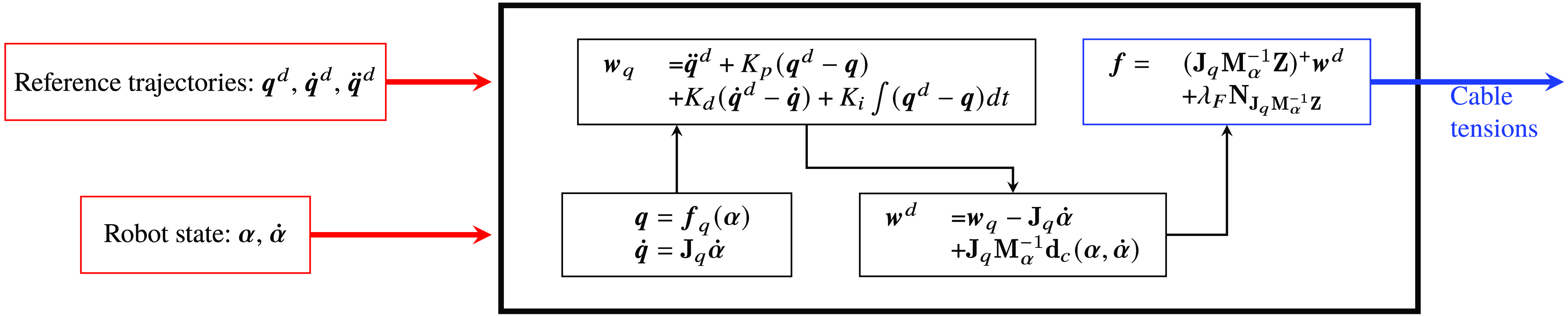
This equation serves as the foundation for our closed-loop control. The objective is to control the cable tensions to achieve the desired trajectory while making the necessary corrections. A PID controller is used to define the corrected acceleration $\boldsymbol{w}_{q}$ as follows:

(10) \begin{equation} \boldsymbol{w}_{q}=\ddot{\boldsymbol{q}}^d+K_p(\boldsymbol{q}^d-\boldsymbol{q})+K_d(\dot{\boldsymbol{q}}^d-\dot{\boldsymbol{q}})+K_i\int (\boldsymbol{q}^d-\boldsymbol{q})dt \end{equation}

where $K_p$ , $K_d$ , and $K_i$ are constants. To ensure stable tracking without oscillations, we set these constants to $K_p=3\omega ^2$ , $K_d=3\omega$ , and $K_i=\omega ^3$ , where $\omega$ is a constant value defined by the user.

The set of cable tensions that produces the corrected acceleration is calculated by

(11) \begin{equation} \boldsymbol{f}=\left (\mathbf{J}_{q}\mathbf{M}_\alpha ^{-1}\mathbf{Z}(\boldsymbol{\alpha })\right )^+\left (\boldsymbol{w}_{q}-\dot{\mathbf{J}}_{q}\dot{\boldsymbol{\alpha}}+\mathbf{J}_{q}\mathbf{M}_\alpha ^{-1}\mathbf{d}_c(\boldsymbol{\alpha },\dot{\boldsymbol{\alpha}})\right )+\lambda _F\mathbf{N}_{\mathbf{J}_{q}\mathbf{M}_\alpha ^{-1}\mathbf{Z}} \end{equation}

where $\mathbf{N}_{\mathbf{J}_{q}\mathbf{M}_\alpha ^{-1}\mathbf{Z}}$ represents the null space vector of the matrix $\mathbf{J}_{q}\mathbf{M}_\alpha ^{-1}\mathbf{Z}(\boldsymbol{\alpha })$ and $\lambda _F$ is a scalar calculated to ensure that the cable tensions are both minimized and maintained above a minimum tension $f_{min}$ .

The control law scheme is depicted in Figure 5.

Figure 5.

CTC scheme.

3.2. Stability analysis

The stability of underactuated systems can be influenced by the choice of controlled variables, as discussed in [Reference Aoustin, Chevallereau, Glumineau and Moog24, Reference Miu27, Reference Isidori and Grizzle35, Reference Gilbert36]

The local stability of a nonlinear system is assessed by examining the stability of its linearized version around a particular operating point. The stability of the linearized system can be determined by studying its transfer function in the Laplace domain.

3.2.1. Linearization of the dynamic model around an equilibrium configuration

To analyze the stability of the control law, we linearize Eq. (1) around an equilibrium configuration $\boldsymbol{\alpha }_0$ with zero velocity, $\dot{\boldsymbol{\alpha}}_0 = \boldsymbol{0}$ . The resulting equation is

(12) \begin{equation} \mathbf{M}_\alpha (\boldsymbol{\alpha }_0)\ddot{\boldsymbol{\alpha}}+\frac{\partial \left (\mathbf{d}_c(\boldsymbol{\alpha }_0,\dot{\boldsymbol{\alpha}}_0)-\mathbf{Z}(\boldsymbol{\alpha }_0)\,\boldsymbol{f}_0\right )}{\partial \boldsymbol{\alpha }}(\boldsymbol{\alpha }-\boldsymbol{\alpha }_0)+\frac{\partial \mathbf{d}_c(\boldsymbol{\alpha }_0,\dot{\boldsymbol{\alpha}}_0)}{\partial \dot{\boldsymbol{\alpha}}}(\dot{\boldsymbol{\alpha}}-\dot{\boldsymbol{\alpha}}_0)=\mathbf{Z}(\boldsymbol{\alpha }_0)(\boldsymbol{f}-\boldsymbol{f}_0) \end{equation}

where $\boldsymbol{f}_0$ is the cable tensions when $\boldsymbol{\alpha }=\boldsymbol{\alpha }_0$ and $\dot{\boldsymbol{\alpha}}=\dot{\boldsymbol{\alpha}}_0$ . We have

(13) \begin{equation} \mathbf{d}_c(\boldsymbol{\alpha }_0,\dot{\boldsymbol{\alpha}}_0)=\mathbf{Z}(\boldsymbol{\alpha }_0)\,\boldsymbol{f}_0 \end{equation}

We introduce the variables $\boldsymbol{\alpha }_*=\boldsymbol{\alpha }-\boldsymbol{\alpha }_0$ and $\boldsymbol{f}_*=\boldsymbol{f}-\boldsymbol{f}_0$ and we define matrices as $\mathbf{M}=\mathbf{M}_\alpha (\boldsymbol{\alpha }_0)$ , $\mathbf{K}=\frac{\partial \left (\mathbf{d}_c(\boldsymbol{\alpha }_0,\dot{\boldsymbol{\alpha}}_0)-\mathbf{Z}(\boldsymbol{\alpha }_0)\,\boldsymbol{f}_0\right )}{\partial \boldsymbol{\alpha }}$ , $\mathbf{D}=\frac{\partial \mathbf{d}_c(\boldsymbol{\alpha }_0,\dot{\boldsymbol{\alpha}}_0)}{\partial \dot{\boldsymbol{\alpha}}}$ . This leads to the equation:

(14) \begin{equation} \mathbf{M}\ddot{\boldsymbol{\alpha}}_*+\mathbf{D}\dot{\boldsymbol{\alpha}}_*+\mathbf{K}\boldsymbol{\alpha }_*=\mathbf{Z}(\boldsymbol{\alpha }_0)\,\boldsymbol{f}_* \end{equation}

Controlling the cable tension to maintain positivity is a nonlinear aspect of the control law. As discussed in Section 2.3, the robot configuration may depend on the minimum tension imposed. To simplify the analysis, we consider degenerate cases in which the robot configuration is not influenced by the minimum tension. These cases also allow us to work with reduced torques:

(15) \begin{equation} \mathbf{M}\ddot{\boldsymbol{\alpha}}_*+\mathbf{D}\dot{\boldsymbol{\alpha}}_*+\mathbf{K}\boldsymbol{\alpha }_*= \mathbf{T} \boldsymbol{\Gamma }_* \end{equation}

where $\boldsymbol{\Gamma }_*=\boldsymbol{\Gamma }-\boldsymbol{\Gamma }_0$ such that $\mathbf{Z}(\boldsymbol{\alpha }_0)\,\boldsymbol{f}_0=\mathbf{T}\boldsymbol{\Gamma }_0$ .

Finally, the controlled variables can be linearized as

(16) \begin{equation} \boldsymbol{q}=\boldsymbol{q}_{0}+\mathbf{J}_{q}(\boldsymbol{\alpha }_0)(\boldsymbol{\alpha }-\boldsymbol{\alpha }_0) \end{equation}

By defining $\boldsymbol{q}_{*}=\boldsymbol{q}-\boldsymbol{q}_{0}$ , we have

(17) \begin{equation} \boldsymbol{q}_{*}=\mathbf{J}_{q}(\boldsymbol{\alpha }_0)\boldsymbol{\alpha }_* \end{equation}

3.2.2. Transfer function

Once the equations are linearized, they can be expressed in the Laplace domain. Equations (15) and (17) become:

(18) \begin{equation} \mathbf{M}s^2\tilde{\boldsymbol{A}}+\mathbf{D}s\tilde{\boldsymbol{A}}+\mathbf{K}\tilde{\boldsymbol{A}}=\mathbf{T} \tilde{\boldsymbol{\Gamma }} \end{equation}

(19) \begin{equation} \tilde{\boldsymbol{Q}}=\mathbf{J}_{q}\tilde{\boldsymbol{A}} \end{equation}

where $s$ is the Laplace variable and $\tilde{\boldsymbol{A}}$ , $\tilde{\boldsymbol{\Gamma }}$ , and $\tilde{\boldsymbol{Q}}$ , correspond to $\boldsymbol{\alpha }_*$ , $\boldsymbol{\Gamma }_*$ , and $\boldsymbol{q}_*$ in the Laplace domain. These equations lead to:

(20) \begin{equation} \mathbf{K}_D(s)\tilde{\boldsymbol{A}}=\mathbf{T}\tilde{\boldsymbol{\Gamma }} \end{equation}

where $\mathbf{K}_D(s)=\mathbf{M}s^2+\mathbf{D}s+\mathbf{K}$ .

Then:

(21) \begin{equation} \tilde{\boldsymbol{Q}}=\mathbf{H}_{q}(s)\tilde{\boldsymbol{\Gamma }} \end{equation}

where $\mathbf{H}_{q}(s)=\mathbf{J}_{q}\mathbf{K}_D^{-1}(s)\mathbf{T}$

The control law is designed so that the acceleration $\ddot{\boldsymbol{q}}$ corresponds to the one defined in (10). Thus, the transfer function between $\boldsymbol{q}$ and $\boldsymbol{Q}^{\boldsymbol{d}}$ is

(22) \begin{equation} \tilde{\boldsymbol{Q}}=\tilde{\boldsymbol{Q}}^{\boldsymbol{d}} \end{equation}

If we define the transfer function between $\tilde{\boldsymbol{\Gamma }}$ and $\tilde{\boldsymbol{Q}}^d$ as

(23) \begin{equation} \tilde{\boldsymbol{\Gamma }}=\mathbf{G}(s)\tilde{\boldsymbol{Q}}^d \end{equation}

Then the transfer function between $\boldsymbol{q}$ and $\boldsymbol{q}^d$ is

(24) \begin{equation} \tilde{\boldsymbol{Q}}=\mathbf{H}_{q}(s)\mathbf{G}(s)\tilde{\boldsymbol{Q}}^d \end{equation}

Since the control law is established to satisfy Eq. (22), it follows that

(25) \begin{equation} \mathbf{G}(s)=\mathbf{H}_{q}^{-1}(s). \end{equation}

This expression means that the control law fully compensates for the dynamic model, and in the absence of perturbations, if the model is perfectly identified, the controlled variables will precisely follow their desired trajectories. The zeros of $\mathbf{H}_{q}$ correspond to the poles of $\mathbf{G}(s)$ . Here, $\mathbf{G}(s)$ is a matrix whose terms are rational fractions. The numerators may vary but the denominators are the same for all terms. The control law will be stable if all the poles of $\mathbf{G}(s)$ have a strictly negative real part.

3.3. Results of the computed torque control stability

In this section, we examine the stability of the CTC for robots with progressively more joints, ranging from 2 to 6 modules. To handle less variables, the analysis is carried out in degenerate cases.

The relationship between the acceleration of the controlled variables and the reduced torques at the equilibrium configuration can be derived from the dynamic model (9) as follows:

(26) \begin{equation} \ddot{\boldsymbol{q}}=\mathbf{J}_{q}\mathbf{M}_\alpha ^{-1} \mathbf{T}\boldsymbol{\Gamma } - \mathbf{J}_{q}\mathbf{M}_\alpha ^{-1}\mathbf{d}_c(\boldsymbol{\alpha },\dot{\boldsymbol{\alpha}}) + \dot{\mathbf{J}}_{q}\dot{\boldsymbol{\alpha}} \end{equation}

From this equation, the relationship between the reduced torques $\boldsymbol{\Gamma }$ applied by the cables around the joints and the acceleration of the controlled variables can be described by

(27) \begin{equation} \mathbf{B}_{q}=\mathbf{J}_{q}\mathbf{M}_\alpha ^{-1}\mathbf{T}. \end{equation}

The static model can be linearized from (15), which leads to:

(28) \begin{equation} \mathbf{K}\Delta \boldsymbol{\alpha }=\mathbf{T}\Delta \boldsymbol{\Gamma } \quad \Longrightarrow \quad \Delta \boldsymbol{q}= \mathbf{J}_{q}\mathbf{K}^{-1} \mathbf{T}\Delta \boldsymbol{\Gamma } \end{equation}

The relationship between variations in the positions of the controlled variables and changes in cable tensions in statics can be described by

(29) \begin{equation} \mathbf{K}_{q}=\mathbf{J}_{q}\mathbf{K}^{-1}\mathbf{T}. \end{equation}

The effect of a force on the static model and on the acceleration is analyzed from the expressions of the two matrices $\mathbf{B}_{q}$ and $\mathbf{K}_{q}$ introduced above.

3.3.1. Robot with 2 joints and 2 cables

This section focuses on the robot depicted in Figure 2 a, which has 2 joints and 2 cables. The springs associated with the joints on both the left and right sides have a stiffness of 400 N/m. With 2 cables, it is possible to control only one DoF. Moreover, in static equilibrium, the angles $\alpha _1$ and $\alpha _2$ take the same value denoted as $\alpha _R = \alpha _I = \alpha _1 = \alpha _2$ .

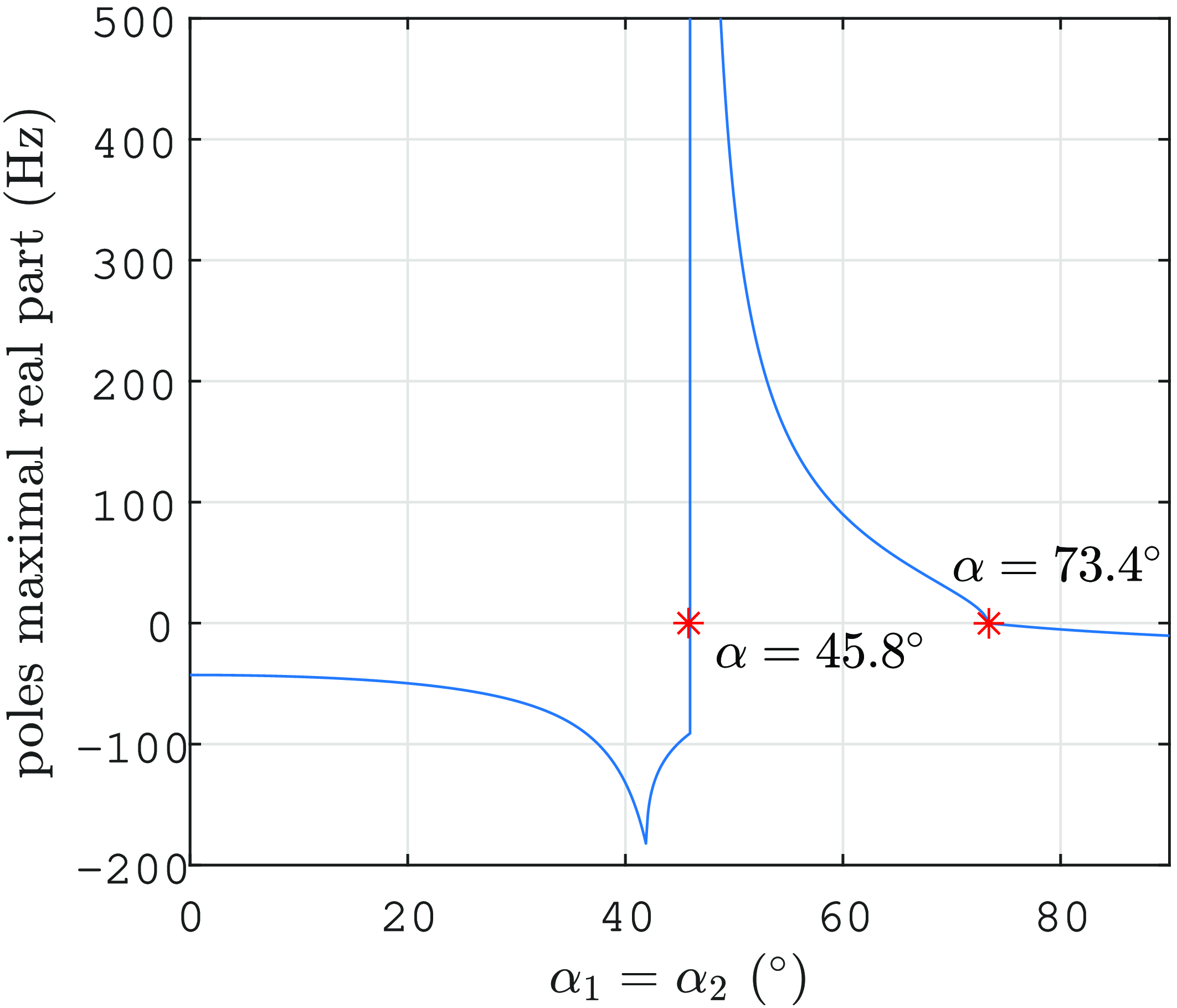
The maximum real part of the poles of $\mathbf{G}(s)$ is consistently negative for the control of either $\boldsymbol{q}=y$ or $\boldsymbol{q}=\gamma$ . As a result, these control strategies remain stable around all joint values $\alpha _I$ .

We now study the control of $\boldsymbol{q}=x$ . Figure 6 shows the plot of the maximum real part of the transfer function poles for 0 $\le$ $\alpha _I$ $\le$ 90 $^\circ$ . Symmetric values can be observed for negative $\alpha _I$ . The maximum real part of the transfer function poles becomes positive from 45.8 $^\circ$ to 73.4 $^\circ$ . Consequently, the control strategy is unstable whenever $\alpha _I$ $\in$ [45.8 $^\circ$ , 73.4 $^\circ$ ].

Figure 6.

Plot of the maximal real part of the transfer function poles against the joint angle for the control of $\boldsymbol{q}=x$ for a robot with 2 joints and 2 cables with the CTC.

A study similar to the one presented in ref. [Reference Testard, Chevallereau and Wenger37] can provide a physical interpretation of the instability boundaries for controlling $\boldsymbol{q}=x$ where the control of $\alpha _1$ or $\alpha _2$ for this robot is explored.

For the case at hand, a single-input, single-output (SISO) system, the two matrices introduced above $\mathbf{B}_{q}$ and $\mathbf{K}_q$ are in fact two scalars $B_q$ and $K_q$ , respectively.

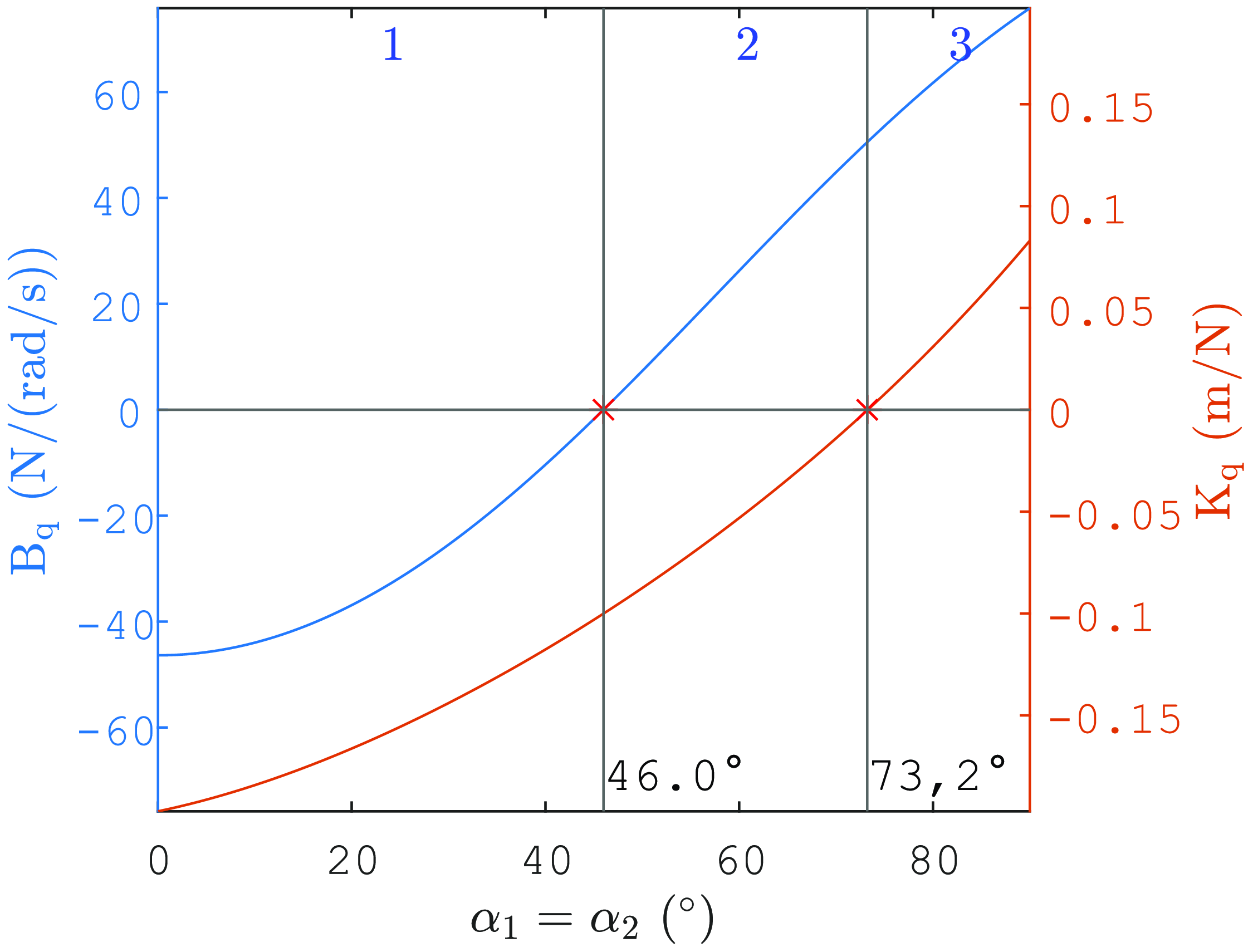
The plots of $B_q$ and $K_q$ against $\alpha _I$ are depicted in Figure 7. These plots reveal three distinct zones: zone 1, where both $B_q$ and $K_q$ are negative, zone 2, where $B_q$ is positive, while $K_q$ remains negative and zone 3, where both $B_q$ and $K_q$ are positive. It is noteworthy that the values of $\alpha _I$ that mark the transitions between these zones closely align with the boundaries of the stability regions shown in Figure 6.

Figure 7.

Plots of $B_q$ and $K_q$ for $\boldsymbol{q}=x$ against the joint angle for a robot with 2 joints and 2 cables.

From Figure 7, it becomes clear that within zones 1 and 3, the cable tensions lead to accelerations of the controlled variable that align with the direction of its static position change. Conversely, in zone 2, the accelerations caused by the cables act in opposition to the static position change.

Therefore, the instability of the control law is associated with the phenomenon where, instantaneously, the controlled variable experiences acceleration in one direction, but subsequently, the static forces lead it to move and converge in the opposite direction, as verified experimentally in ref. [Reference Testard, Chevallereau and Wenger37]. Because of this phenomenon, a PID correction on the acceleration applied within a CTC approach would cause control divergence.

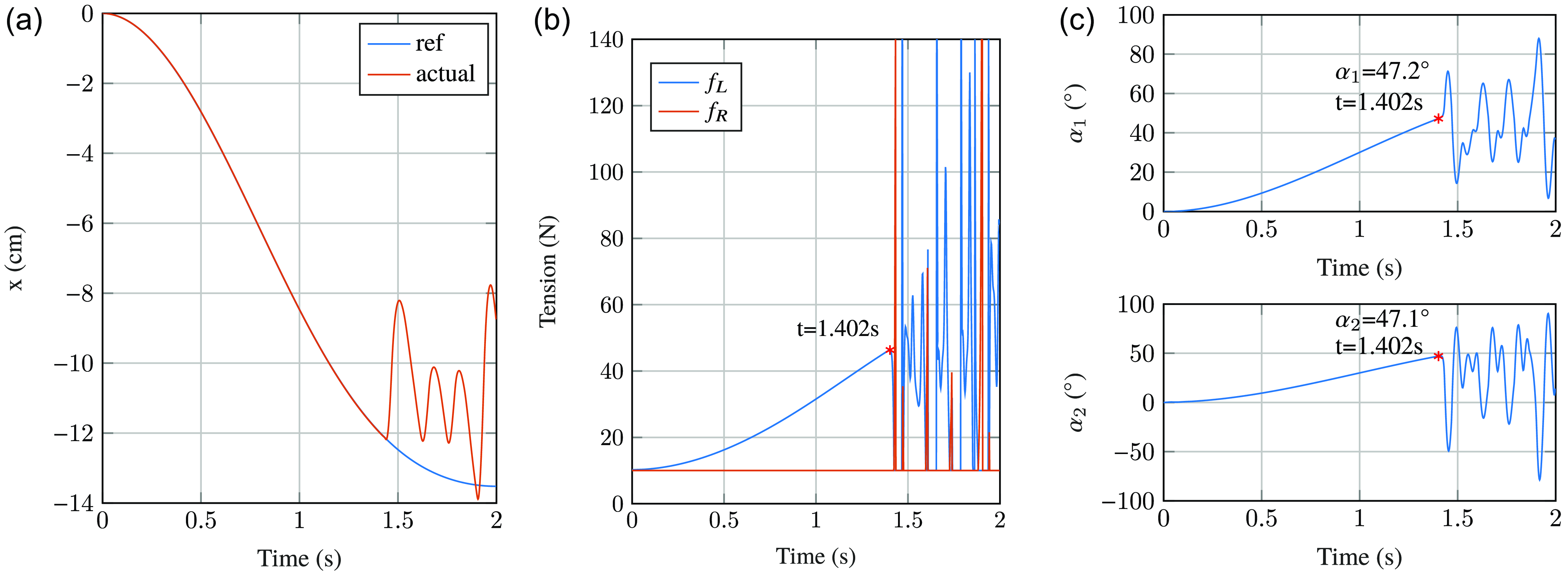
To illustrate the joint limits associated with stability, simulations have been conducted. In Figure 8, a scenario in which $\boldsymbol{q}=x$ is shown. We set the tension saturation in the cables at 140N, $f_{min}=$ 10N and $\omega$ was fixed to 10. The simulation shows that the control remains stable initially as the robot moves. However, instability becomes evident at a particular position, marked by cable tension divergence. The corresponding angles at which instability occurs are approximately $[\alpha _1,\alpha _2]=[47.2^\circ, 47.1^\circ ]^\top$ . While these angles are not exactly equal due to dynamic effects, they are in close proximity to the previously identified stability limit of 45.8 $^\circ$ obtained from the transfer function analysis.

Figure 8.

Simulation of the control of $\boldsymbol{q}=x$ for a robot with 2 joints and 2 cables with the CTC. (a) Corresponds to the tracking of $x$ over time, (b) illustrates the evolution of cable tension over time, and (c) shows the evolution of joint angles over time.

3.3.2. Robot with 3 joints and 3 cables

In this section, we investigate a robot featuring 3 joints and 3 cables, as shown in Figure 2 b. With $N_c=3$ cables, this robot can control 2 DoFs. The springs on the left and right sides of the first two joints have a stiffness of 600 N/m, while the third joint has springs with a stiffness of 300 N/m. A degenerate robot is studied such that $\alpha _I=\alpha _1=\alpha _2$ and $\alpha _{II}=\alpha _3$ in statics.

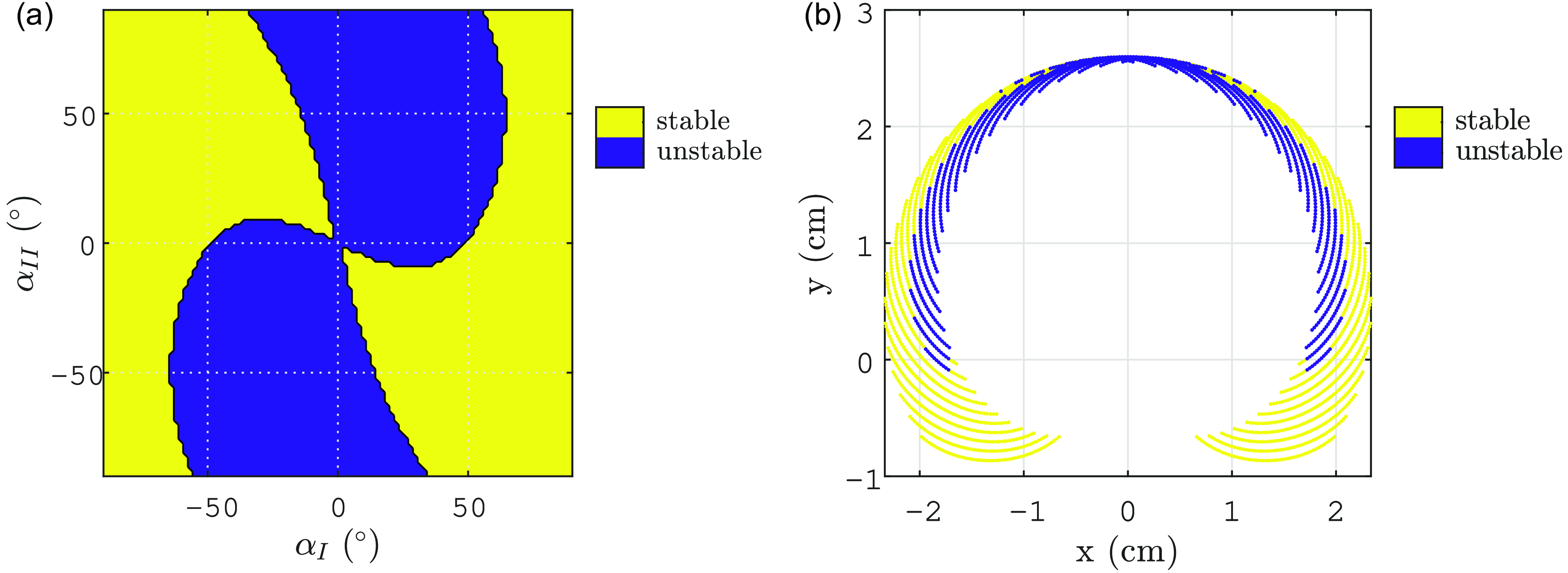
The control stability for $\boldsymbol{q}=[x,y]^\top$ is analyzed with respect to $\alpha _I$ and $\alpha _{II}$ , and the results are shown in Figure 9. This figure depicts the regions of stability and instability as the joint space is scanned. Yellow zones indicate stable control, while blue zones indicate unstable control. The stability/instability regions are plotted both in the joint space and in the controlled variable space.

Figure 9.

Stability domains of the control of $\boldsymbol{q}=[x,y]^\top$ for a robot with 3 joints and 3 cables (a) In the joint space and (b) In the controlled variables space for the CTC.

The analysis shows that CTC exhibits instability across a significant portion of the workspace. The control is stable mainly in positions where $\alpha _I$ has the opposite sign to $\alpha _{II}$ . Moreover, there is a central symmetry in control stability in the joint space, corresponding to axial symmetry in the controlled variables space. The two symmetric zones where the control is stable in the controlled variable space are depicted in Figure 9 b. It is apparent that the largest stable regions are located at the bottom extremities.

Here, our system is multiple-input multiple-output (MIMO) and both $\mathbf{B}_{q}$ and $\mathbf{K}_{q}$ are matrices here. Analyzing the stability results with $\mathbf{B}_{q}$ and $\mathbf{K}_{q}$ becomes then more intricate.

3.3.3. Robots with 6 joints and 4 cables

For the robot with 4 cables (Figure 2 c), the stability study is conducted for the control of $\boldsymbol{q}=[x,y,\gamma ]^\top$ . This study is performed in the absence of gravity, and the joints in the same metamodules have symmetric springs. Specifically, the spring stiffness is 1000 N/m, 800 N/m, and 400 N/m for the first, second, and third metamodule, respectively.

The stability domains, plotted in Figure 10, show that the control of $\boldsymbol{q}=[x,y,\gamma ]^\top$ as function of $\boldsymbol{\alpha} _R$ is almost always unstable. Some small stability regions can be observed.

Figure 10.

Stability domains of the control of $\boldsymbol{q}=[x,y,\gamma ]^\top$ for a robot with 6 joints and 4 cables in the joint space for the CTC.

As the number of joints increases, the CTC exhibits greater instability when applied to the control of EE position and orientation. This observed instability is primarily due to the non-minimum phase nature of the open-loop system for these specific controlled variables.

This study can be extended to the nondegenerate case. The main difference from the degenerate case is that there is a coupling between the choice of forces and the configuration achieved for the same EE pose, as shown in Figures 3 and 4. In linearizing the closed-loop model for the degenerate case, we used the uniqueness of the joint configuration for a given EE pose to explicitly ignore the choice of applied force. This allowed us to use Eq. (5) with a matrix $\mathbf{T}$ of rank $N_c$ . In the nondegenerate case, this is no longer possible. We must then explicitly consider the choice of forces by the controller. The minimum forces are chosen such that each force is greater or equal to $f_{min}$ . Thus, we have at least one force equal to $f_{min}$ . In the linearization, we assume that the same cable will remain at $f_{min}$ in Eq. (14), and $\mathbf{Z}(\boldsymbol{\alpha }_0)\,\boldsymbol{f}_*$ is replaced by $\mathbf{B}\boldsymbol{u}$ , where $\mathbf{B}$ and $\boldsymbol{u}$ represent $\mathbf{Z}(\boldsymbol{\alpha }_0)$ and $\boldsymbol{f}_*$ , respectively, with the rows (resp. lines) corresponding to the cables that are not at the minimal tension $f_{min}$ . If several forces are at $f_{min}$ , several linearizations have to be considered. Using this method, results obtained for the nondegenerate case are close to the results obtained for degenerate robots as it will be shown for the robot with three modules in Section 5.

4.1. Presentation

The CTC instability is attributed to the non-minimum phase nature of the open-loop system. To address this issue, we seek to design a control law that avoids the direct inversion of the dynamic model. The primary objective is to achieve stability across a broader workspace, without the need for full model compensation, while still controlling EE pose variables.

To achieve this objective, we reformulate the dynamic equation (1) in terms of the acceleration of the controlled variables as follows:

(30) \begin{equation} \mathbf{M}_\alpha \left (\mathbf{J}_{q}^+(\ddot{\boldsymbol{q}}-\dot{\mathbf{J}}_{q}\dot{\boldsymbol{\alpha}})+\mathbf{N}_{J_{q}}\boldsymbol{\lambda }_\alpha \right )+\mathbf{d}_c(\boldsymbol{\alpha },\dot{\boldsymbol{\alpha}})=\mathbf{Z}(\boldsymbol{\alpha })\,\boldsymbol{f} \end{equation}

where $\mathbf{N}_{J_{q}}$ is a matrix of the null space vectors of the $\mathbf{J}_{q}$ matrix, and $\boldsymbol{\lambda }_\alpha$ is a $N_j-N_c+1$ vector. The core principle of the control law is to compute an joint acceleration that achieve the desired EE task and then to deduce the appropriate cables tension. To achieve this goal, we set $\lambda _\alpha$ to zero in order to be able to remain stationary at equilibrium configuration. This choice limits internal motions. Even if the obtained joint accelerations is not physically realizable by the actuators, we will show that the control will converge to the desired $\boldsymbol{q}^d$ .

Equation (30) defines a system of $N_j$ equations in $N_c$ unknowns (the components of $\boldsymbol{f}$ ), whereas the number of controlled variables is $N_c-1$ . This discrepancy highlights the impossibility of simultaneously satisfying all these equations. Although the use of the pseudo-inverse of $\mathbf{Z}$ would minimize the disparity between the equations that can or cannot be satisfied, it would not guarantee that the cable tensions are greater than $f_{min}$ . To address this issue, we project these equations onto a lower-dimensional space of dimension $N_c-1$ . By doing so, we can choose $\boldsymbol{f}$ that satisfies the $N_c-1$ equations such that all its components are greater than $f_{min}$ . The projection is performed using a matrix $\mathbf{P}$ that consists of those $N_c-1$ left-singular vectors of the $\mathbf{Z}$ matrix, which are associated with the largest singular values. Notably, the last singular value is primarily related to the internal motion linked to variations in cable tension as illustrated in Figures 3 and 4. In degenerate cases, this singular value is zero, while in general cases, it is small compared to the other singular values.

The resulting equation can be expressed as

(31) \begin{equation} \mathbf{P}\left (\mathbf{M}_\alpha \mathbf{J}_{q}^+(\ddot{\boldsymbol{q}}-\dot{\mathbf{J}}_{q}\dot{\boldsymbol{\alpha}})+\mathbf{d}_c(\boldsymbol{\alpha },\dot{\boldsymbol{\alpha}})\right )=\mathbf{P}\mathbf{Z}(\boldsymbol{\alpha })\,\boldsymbol{f} \end{equation}

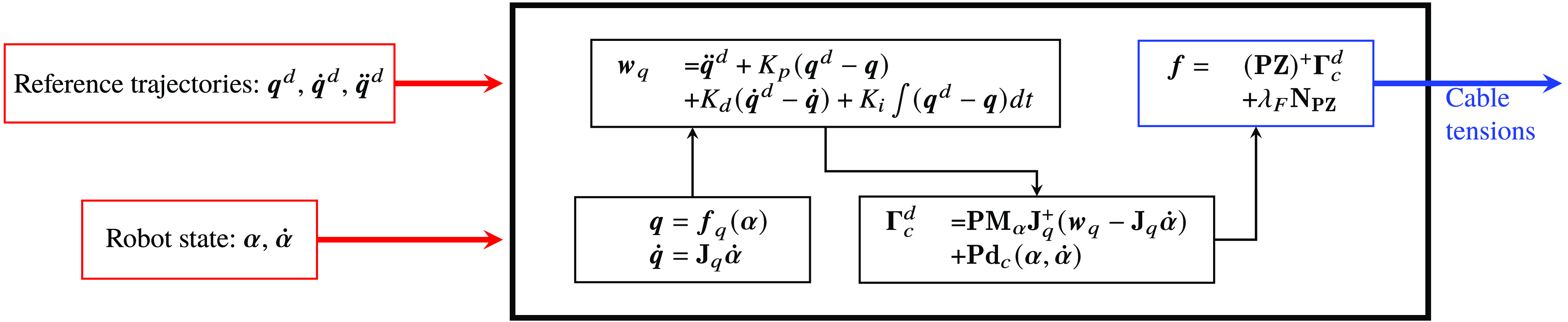
In a manner analogous to the CTC, this equation is employed in a closed-loop control scheme for cable tension computation:

(32) \begin{equation} \boldsymbol{f}=\left (\mathbf{P}\mathbf{Z}(\boldsymbol{\alpha })\right )^+\left ( \mathbf{P}\mathbf{M}_\alpha \mathbf{J}_{q}^+(\boldsymbol{w}_{q}-\dot{\mathbf{J}}_{q}\dot{\boldsymbol{\alpha}})+\mathbf{P}\mathbf{d}_c(\boldsymbol{\alpha },\dot{\boldsymbol{\alpha}})\right )+\lambda _F\mathbf{N}_{\mathbf{P}\mathbf{Z}} \end{equation}

where $\mathbf{N}_{\mathbf{P}\mathbf{Z}}$ represents the null space vector of the $\mathbf{P}\mathbf{Z}$ matrix.

The control architecture is visually depicted in Figure 11.

Figure 11.

PCTC scheme.

4.2. Transfer function

Similar to the CTC approach, the stability of the control law can be assessed with the same methodology. In the Laplace domain, for a degenerate case, the closed-loop dynamic equation derived from Eqs. (31) and (10) can be expressed as follows:

(33) \begin{equation} \mathbf{P}\mathbf{M}\mathbf{J}_{q}^+(s^2\tilde{\boldsymbol{Q}}^d+PID(s)(\tilde{\boldsymbol{Q}}^d-\tilde{\boldsymbol{Q}}))+\mathbf{P}(\mathbf{K}+\mathbf{D}s)\tilde{\boldsymbol{A}}=\mathbf{P}\mathbf{T}\tilde{\boldsymbol{\Gamma }} \end{equation}

To analyze the stability of the control law, it is necessary to define the closed-loop transfer function $\mathbf{G}_2(s)$ that connects $\tilde{\boldsymbol{\Gamma }}$ to $\tilde{\mathbf{Q}}^d$ . Equation (33) can be rearranged as

(34) \begin{equation} \mathbf{P}\mathbf{T}\tilde{\boldsymbol{\Gamma }}-\mathbf{P}(\mathbf{K}+\mathbf{D}s)\tilde{\boldsymbol{A}}+\mathbf{P}\mathbf{M}\mathbf{J}_{q}^+PID(s)\tilde{\boldsymbol{Q}}=\mathbf{P}\mathbf{M}\mathbf{J}_{q}^+(s^2+PID(s))\tilde{\boldsymbol{Q}}^d \end{equation}

Subsequently, from Eqs. (20) and (21), we can establish:

(35) \begin{equation} \tilde{\boldsymbol{\Gamma }}=\mathbf{G}_2(s)\tilde{\mathbf{Q}}^d \end{equation}

where

(36) \begin{equation} \mathbf{G}_2(s)=\left (\mathbf{P}\mathbf{T}-\mathbf{P}(\mathbf{K}+\mathbf{D}s)\mathbf{K}_D^{-1}(s)\mathbf{T}+\mathbf{P}\mathbf{M}\mathbf{J}_{q}^+PID(s)\mathbf{H}_{q}\right )^{-1}\mathbf{P}\mathbf{M}\mathbf{J}_{q}^+(s^2+PID(s)) \end{equation}

Using Eq (21), we can compute the transfer function between $\tilde{\boldsymbol{Q}}$ and $\tilde{\boldsymbol{Q}}^d$ as

(37) \begin{equation} \tilde{\boldsymbol{Q}}=\mathbf{H}_{q}(s)\mathbf{G}_2(s)\tilde{\boldsymbol{Q}}^d \end{equation}

It is important to note that $\mathbf{H}_{q}(s)\mathbf{G}_2(s)$ does not form the identity matrix, except at $s=0$ . Consequently, for a step command in the controlled variables space, the motions of the controlled variables converge to their desired values, as per the principle of the final value theorem [Reference Rasof38].

4.3. Results of the stability for the pseudo computed control law

This section performs the stability analysis as Section 3.3 for the PCTC.

4.3.1. Robot with 2 joints and 2 cables

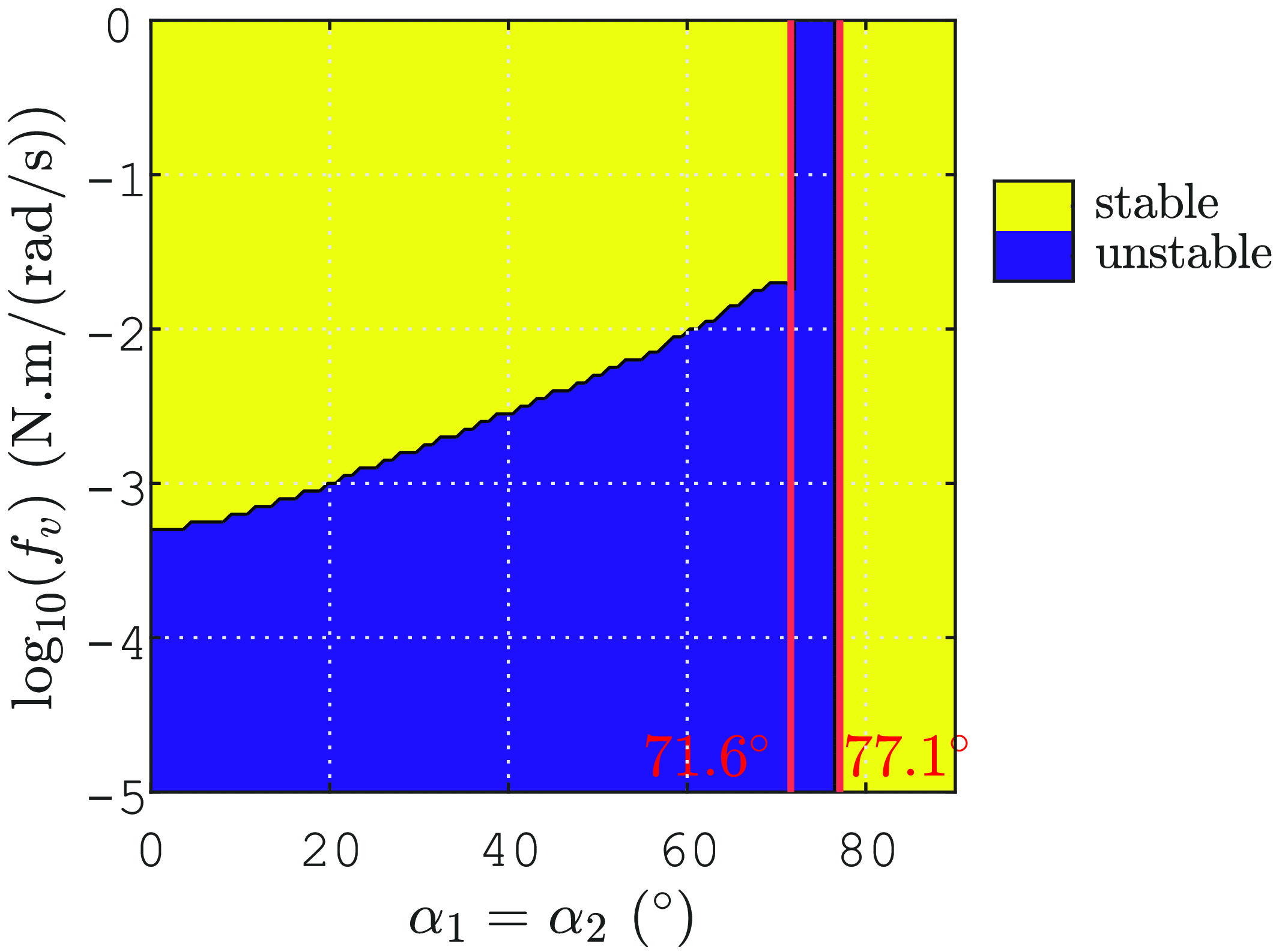
We investigate the control stability of $\boldsymbol{q}=x$ , as depicted in Figure 12.

We observe that control law stability is influenced by viscous friction within the system. More specifically, a minimal viscous friction constant $f_v$ (see Section 2.2) should exist to avoid instability. For the CTC, in contrast, we observed that the value of $f_v$ had no significant impact.

Figure 12 shows that when $f_v$ is not too low, the region of instability shrinks significantly and is confined to the range between $71.6^\circ$ and $77.1^\circ$ ( $5.1\%$ of the joint space), as marked by the two vertical red lines. This contrasts with CTC, where the instability range is wider, between $45.8^\circ$ and $73.4^\circ$ which corresponds to $30.7\%$ of the joint space (see Figure 6). The control of $\boldsymbol{q}=y$ and $\boldsymbol{q}=\gamma$ is always stable, similar to the behavior observed with the CTC.

Figure 12.

Stability domains of the control of $\boldsymbol{q}=x$ for a robot with 2 joints and 2 cables against the robot joint angle and the viscous friction constant for the PCTC.

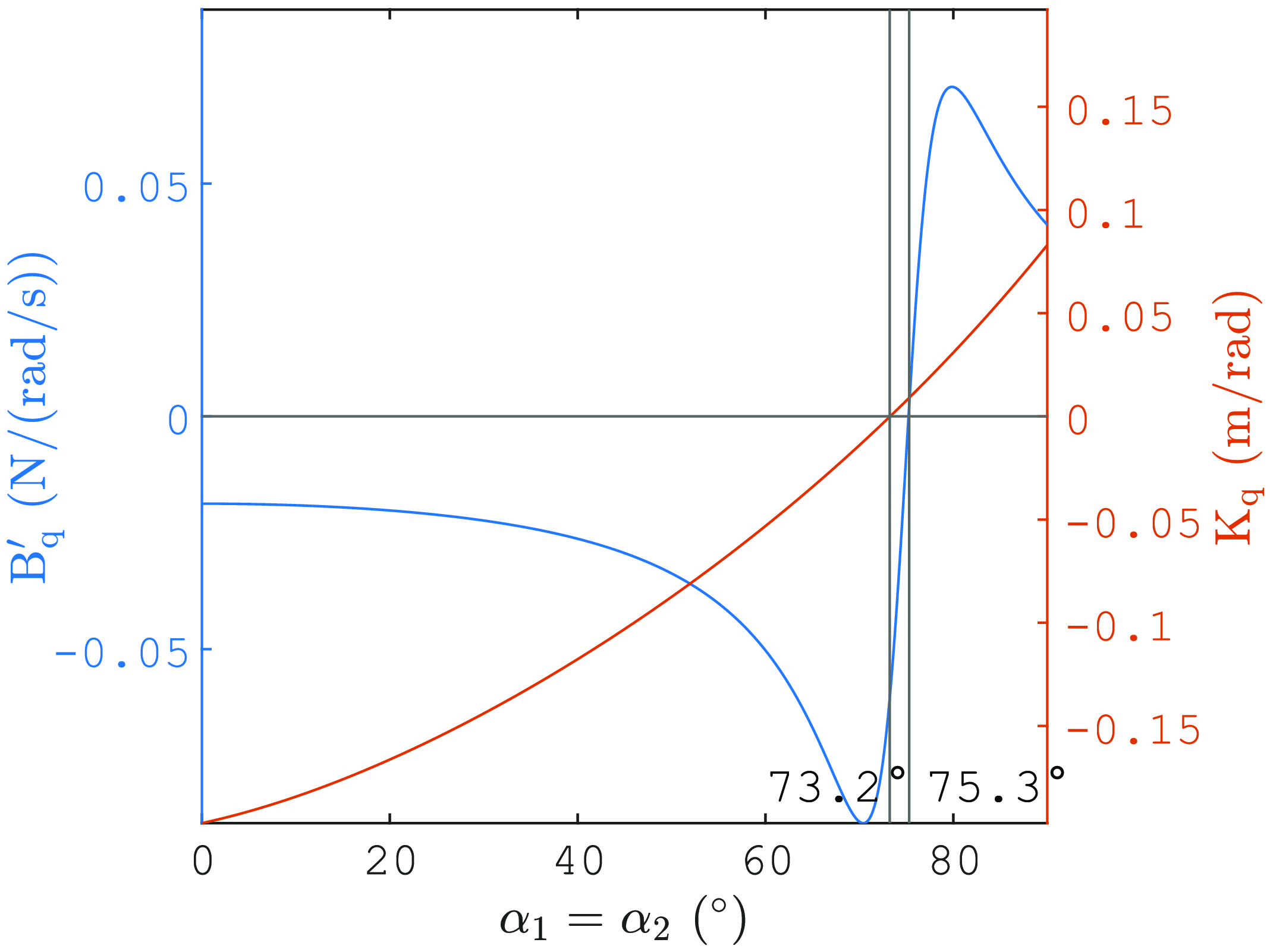
In a manner analogous to the CTC, we introduce a new term, $B_q'=\left (\mathbf{P}\mathbf{M}\mathbf{J}_q^+\right )^{-1}\mathbf{PT}$ , which relates the calculated cable tension to the acceleration of the controlled variables within the PCTC law. Figure 13 shows the plot of $B_q'$ and $K_q$ (as defined in Eq. (29)) against the robot joint angle. It is apparent that the angle values at which $B_q'$ and $K_q$ change their sign are closely related to the angles that delineate the boundaries of the control law stability domain. In fact, the control law is unstable when $B_q'$ and $K_q$ do not have the same sign, as shown in Figure 13. Note that $K_q$ cancels out when $\mathbf{J}_q\mathbf{T}=0$ as $\mathbf{K}$ is a scalar matrix in this case (see Eq. (29)).

Figure 13.

Plot of $B_q'$ and $K_q$ for $\boldsymbol{q}=x$ against the joint angle for a robot with 2 joints and 2 cables.

4.3.2. Robot with 3 joints and 3 cables

Figure 14.

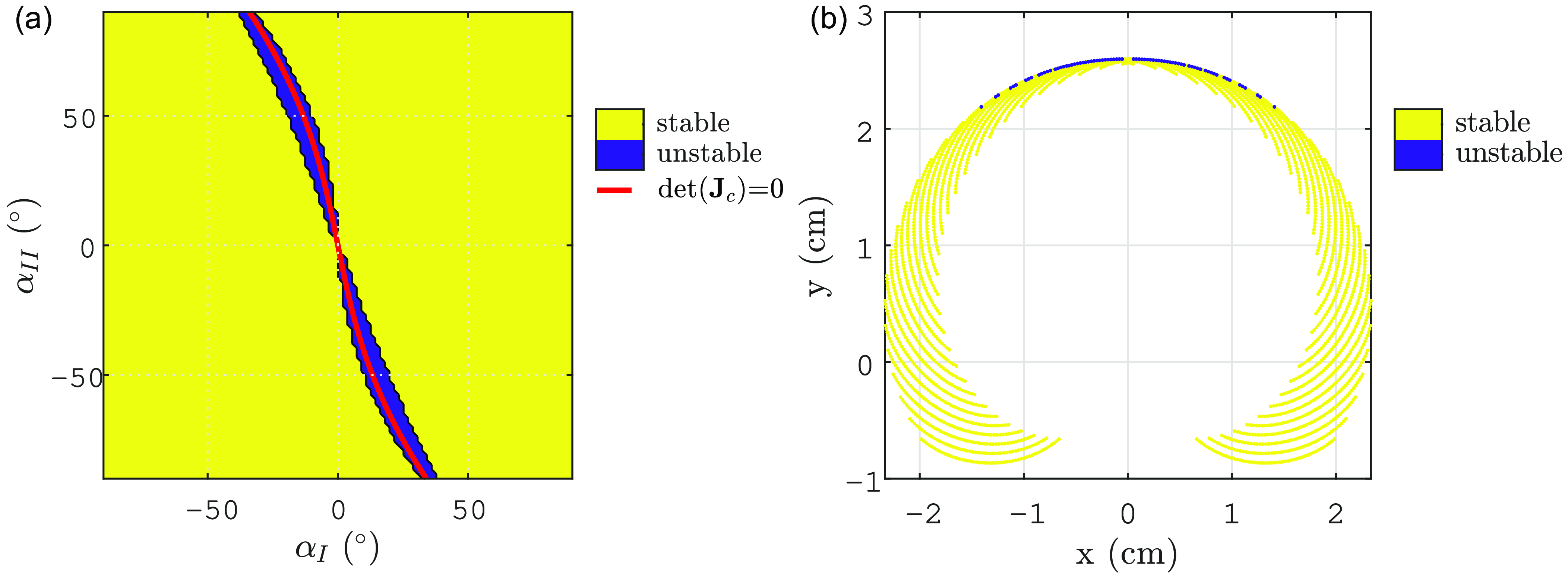
Stability domains of the control of $\boldsymbol{q}=[x,y]^\top$ for a robot with 3 joints and 3 cables (a) In the joint space and (b) In the controlled variables space for the PCTC.

We consider a sufficient viscous friction constant, namely, $f_v = 0.1$ N.m/(rad/s). The stability of PCTC for $\boldsymbol{q} = [x, y]^\top$ is shown in the joint space and controlled variables space in Figure 14. It is evident from these figures that the stability domain of the PCTC covers a larger portion of the joint space, with only $3.1\%$ unstable, compared to that of the CTC, which has $41.8\%$ of the joint space unstable (see Figure 9 a). As with the CTC, the interpretation of the instability by $\mathbf{B}_q'$ and $\mathbf{K}_q$ is not straightforward in the context of this MIMO system. However, a valuable approach is to introduce a Jacobian matrix $\mathbf{J}_c = \mathbf{J}_q\mathbf{T}$ that relates the controlled DoFs and the reduced angles: $\dot{\boldsymbol{q}} = \mathbf{J}_c\dot{\boldsymbol{\alpha}}_R$ . It turns out that the instability area is concentrated in a narrow zone around the singularity curve defined by $det(\mathbf{J}_c) = 0$ (shown in red in Figure 14 a). In the controlled variables space, the instability area is located near the upper workspace boundary (see Figure 14 b). Control stability is more likely to be maintained when the robot operates far from these kinematic singularities.

4.3.3. Robot with 6 joints and 4 cables

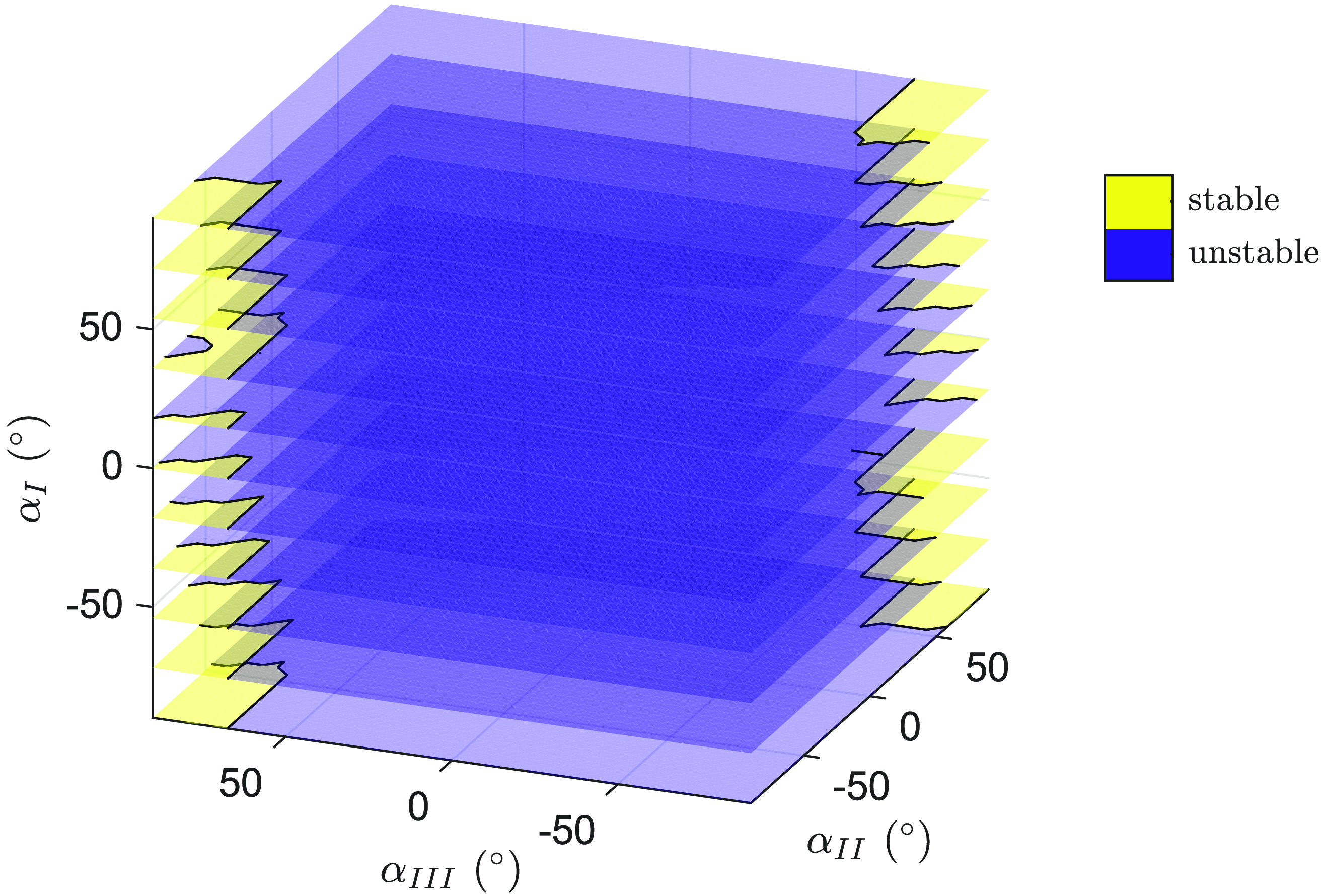
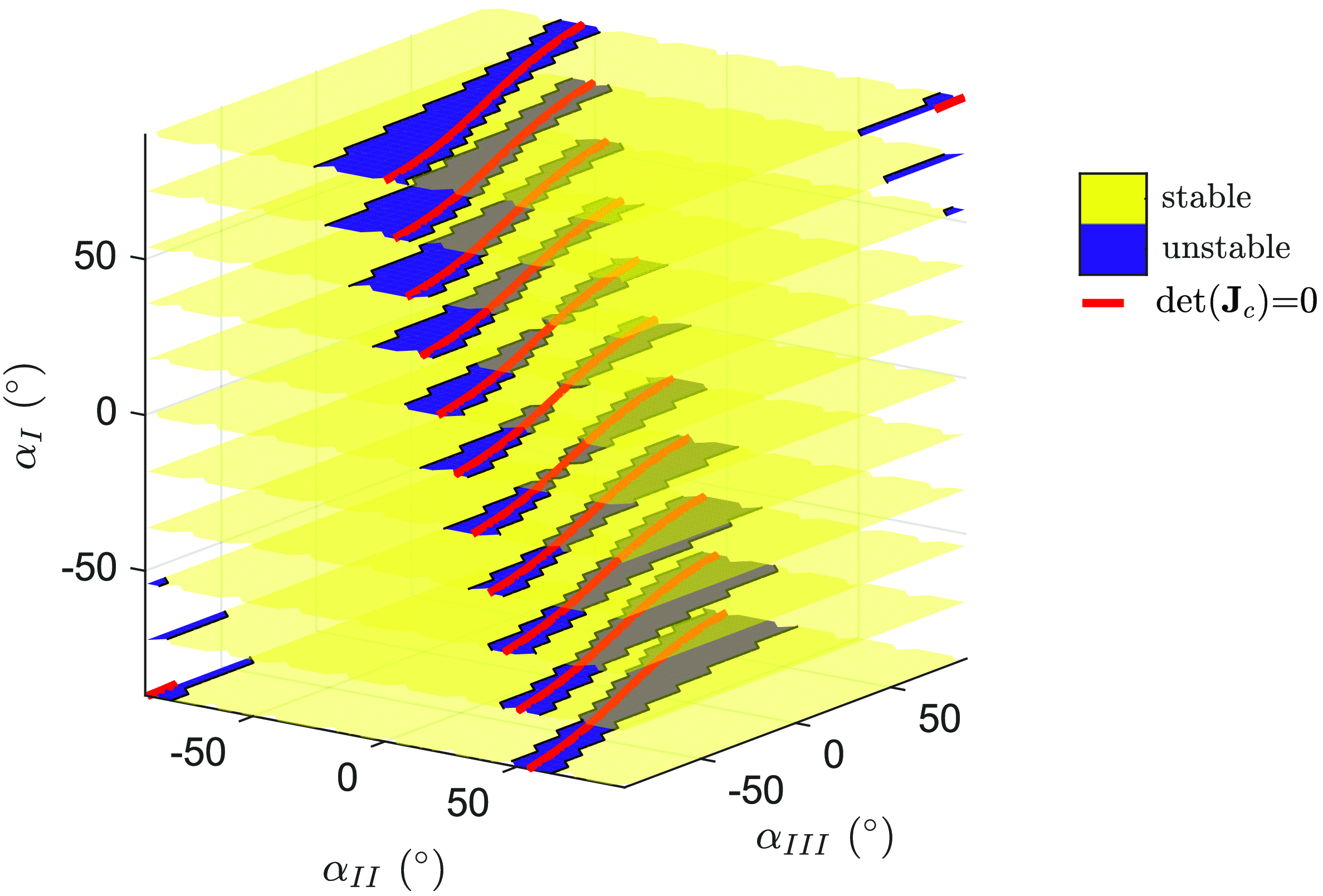
Here, the controlled variables are defined by $\boldsymbol{q}=[x,y,\gamma ]^\top$ . Figure 15 shows the stability analysis in the joint space, plotted at discretized sections of $\alpha _I$ . The stability domain is significantly larger for the PCTC, with approximately $6.7\%$ of the joint space unstable, compared to the CTC, which has approximately $94.2\%$ of the joint space unstable. The small unstability areas of the PCTC are located around the singularities $det(\mathbf{J}_c) = 0$ , as for the two previous robots.

Figure 15.

Stability domains of the control of $\boldsymbol{q}=[x,y,\gamma ]^\top$ for a robot with 6 joints and 4 cables in the joint space for the PCTC.

Using the PCTC effectively reduces the robot internal motions while maintaining reasonable tracking of the controlled variables. Although the calculated accelerations in this approach may not be physically feasible, the control algorithm ensures convergence to the desired evolution of the controlled variables. As a result, it has been observed that this control method provides greater stability than the CTC, especially when the controlled variables are $x$ and $y$ or $x$ , $y$ , and $\gamma$ .

5.1. Prototype description

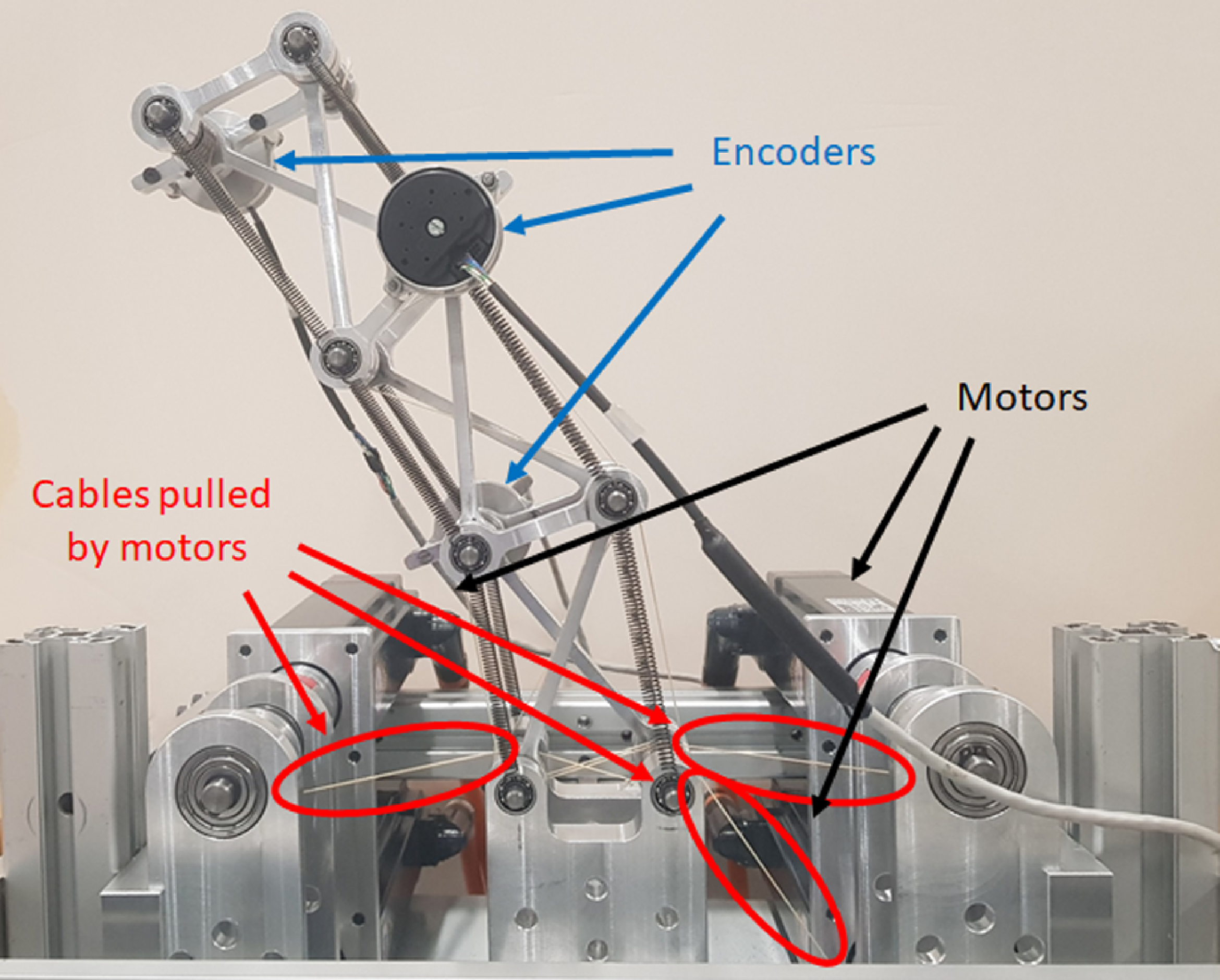
Experiments were conducted on the prototype depicted in Figure 16, which consists of three joints and three cables, like in Figure 2b.

Figure 16.

Prototype.

The prototype specifications are given in Table I. The selection of springs is based on achieving a stable configuration at rest, which is positioned away from kinematic singularities (i.e., without tension cable the prototype joint angles are $\boldsymbol{\alpha }\approx [12.5^\circ, 17.9^\circ, -26.7^\circ ]^\top$ ). Additionally, these chosen springs ensure stability in the control of the EE position at rest with the CTC and PCTC, as shown in Figures 18 and 19.

Table I.

Prototype specifications.

Encoders (Heidenhain ECI 1119), attached to the short bars as shown in Figure 16, measure the angles $\phi _i$ or $\psi _i$ of each X-joint. The alternation between measuring $\phi _i$ (when the encoder is on the left) and $\psi _i$ (when the encoder is on the right) is implemented to mitigate the imbalance in mass distribution. The joint angles $\alpha _i$ are then obtained by Eq. (38).

(38) \begin{equation} \begin{split} \alpha _i&=2atan_2(b-Lcos(\phi _i),Lsin(\phi _i)), \quad i=[1,3]\\ \alpha _i&=2atan_2(-b-Lcos(\psi _i),Lsin(\psi _i)), \quad i=2 \end{split} \end{equation}

5.2. Comparison between CTC and PCTC

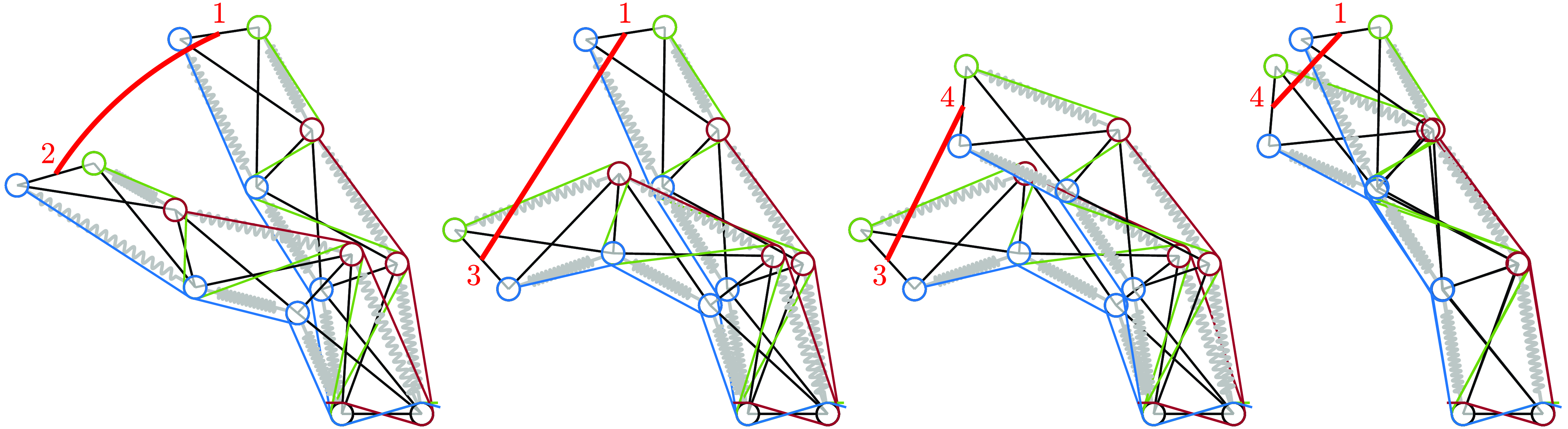
Experiments were conducted for the control of $\boldsymbol{q}=[x,y]^T$ with CTC and PCTC. The studied trajectories are depicted in Figure 17. The first trajectory follows a curved path from configuration 1 to configuration 2. The remaining trajectories consist of straight lines connecting configuration 1 to configuration 3, then from 3 to 4, and finally from 4 back to 1.

Figure 17.

Trajectories of the EE (from 1 to 2, 1 to 3, 3 to 4 and 4 to 1).

Under gravity and with the chosen springs, the system is not in the degenerate case anymore, resulting in the equilibrium configuration being influenced by the minimal cable tension. When considering specified desired values for angles like $\alpha _I=\alpha _1$ and $\alpha _{II}=\alpha _3$ , the determination of static equilibrium, while maintaining minimal cable tension, involves calculating $\alpha _2$ and the associated forces together through an optimization process:

(39) \begin{equation} \begin{split} (\alpha _2,\boldsymbol{f})=&\min _{\alpha _2,\boldsymbol{f}}||\boldsymbol{f}||\\ &s.t.\; \begin{split} & \boldsymbol{d}_c([\alpha _I,\alpha _2,\alpha _{II}]^\top, 0)=\mathbf{Z}([\alpha _I,\alpha _2,\alpha _{II}]^\top )\,\boldsymbol{f}\\ & min(\boldsymbol{f}) \ge f_{min} \end{split} \end{split} \end{equation}

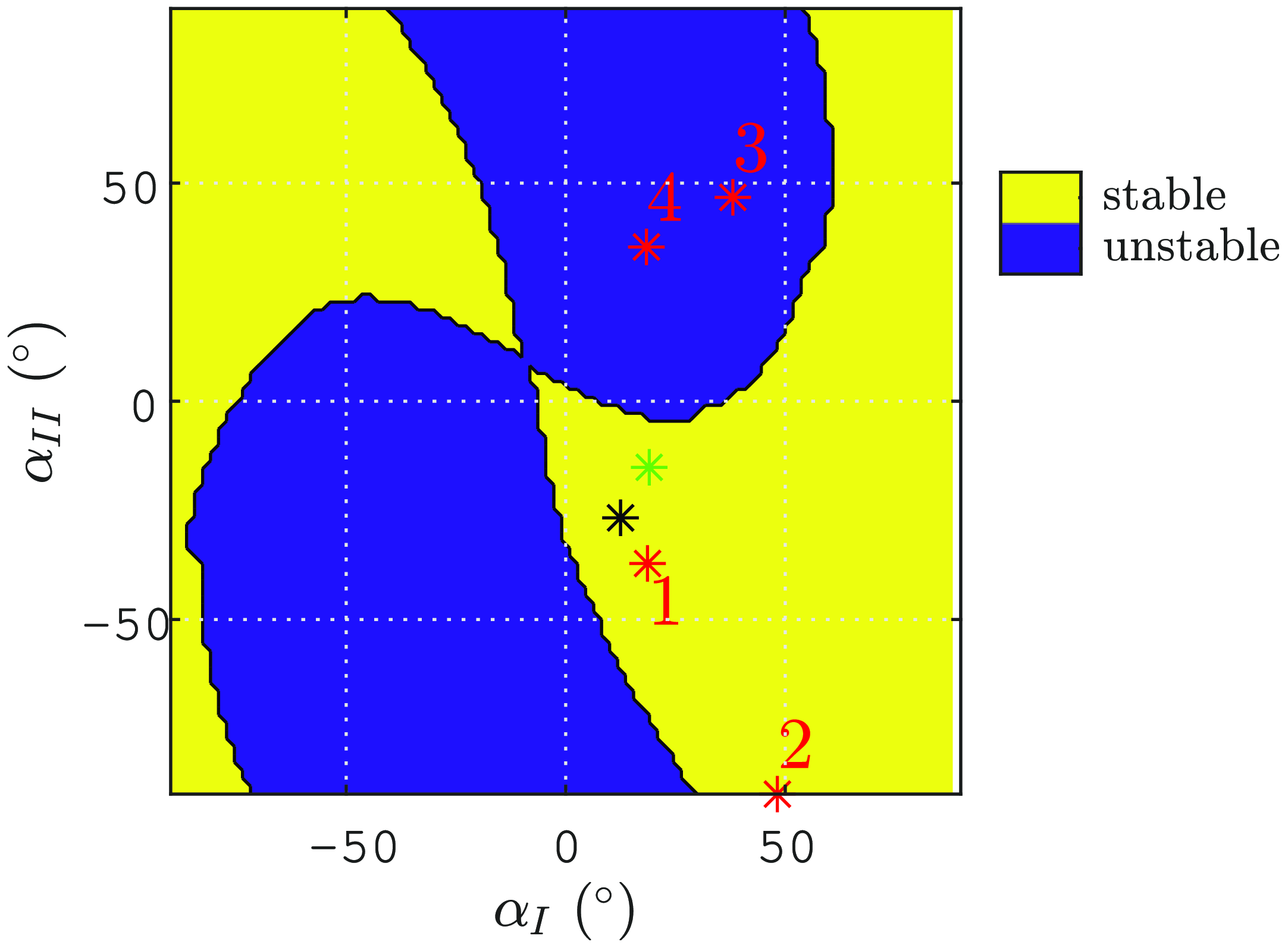
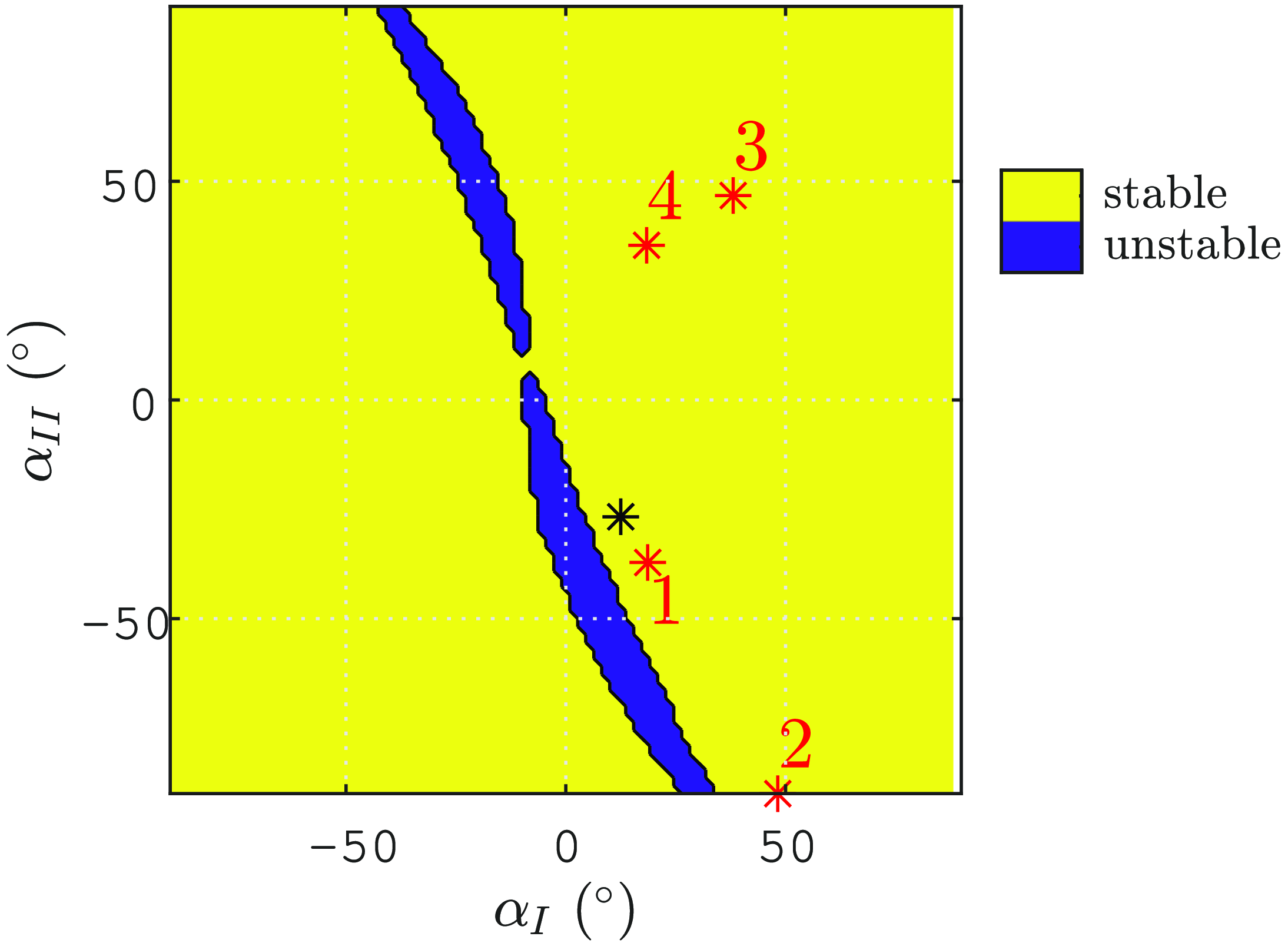
Subsequently, the computation of the $\mathbf{B}$ matrix is performed, as explained toward the end of Section 3.3.3. The obtained results are presented in Figure 18 for the CTC and in Figure 19 for the PCTC. It is noteworthy that similar stability and instability domains are observed as in the degenerate case, as depicted in Figures 9a and 14a. The observed instability domains are not centered on $[\alpha _I,\alpha _{II}]=[0,0]^\top$ due to the fact that equilibrium does not result in $\alpha _1=\alpha _2$ . This behavior is influenced by the springs selected and by gravity.

The different equilibrium configurations in the joint space of our trajectories are represented by red stars in Figures 18 and 19. The configurations 1 and 2 are in the stable zone for the CTC and PCTC, while the configurations 3 and 4 are in the stable zone for the PCTC and unstable zone for the CTC.

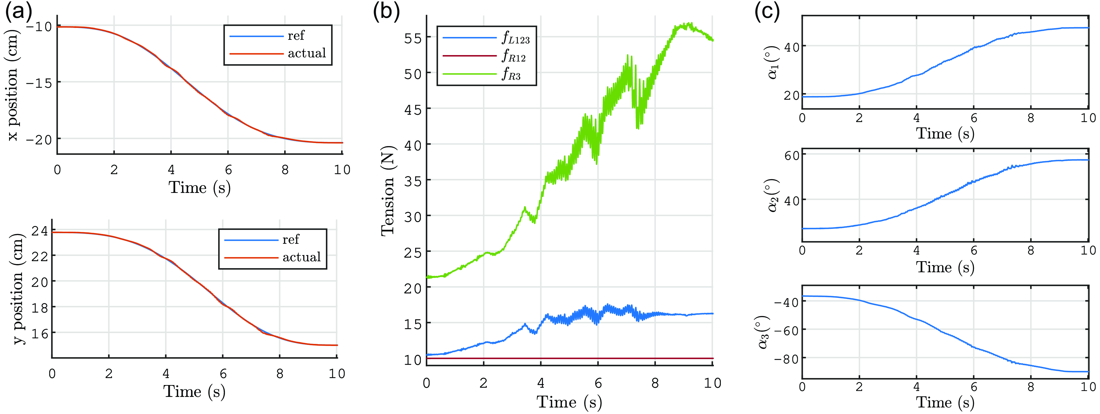
Figure 20 depicts the motion executed with the CTC from the configuration 1 to the configuration 2. Throughout the motion, the robot remains within the stable control domain, showing consistent and stable control behavior. Due to the challenge in accurately identifying nonlinear dry friction in the motors and joints, the PID gain $\omega$ was fine-tuned to achieve precise trajectory tracking (refer to Figure 20 a). Consequently, the oscillations observed in the cable tension are attributed to the effects of these frictions. It is also evident that the tension in all cables is consistently maintained above the desired minimum tension, with one of the cables at the minimum tension level.

Figure 18.

Stability domains of the control of $\boldsymbol{q}=[x,y]^\top$ for a robot with 3 joints and 3 cables under gravity and with the prototype springs in the joint space for the CTC. The red stars correspond to the numbered robot configurations of Figure 17. The black star is the configuration at rest. The green star is the point when the control becomes unstable during motion from 1 to 3.

Figure 19.

Stability domains of the control of $\boldsymbol{q}=[x,y]^\top$ for a robot with 3 joints and 3 cables under gravity and with the prototype springs in the joint space for the PCTC. The red stars correspond to the numbered robot configurations of Figure 17. The black star is the configuration at rest.

Figure 20.

Time histories of (a) $x$ and $y$ , (b) $\mathbf{f}$ , and (c) the $\alpha _i$ for the trajectory from configurations 1 to 2 from with the CTC. For (b), the plot colors correspond to the cable colors in Figure 17.

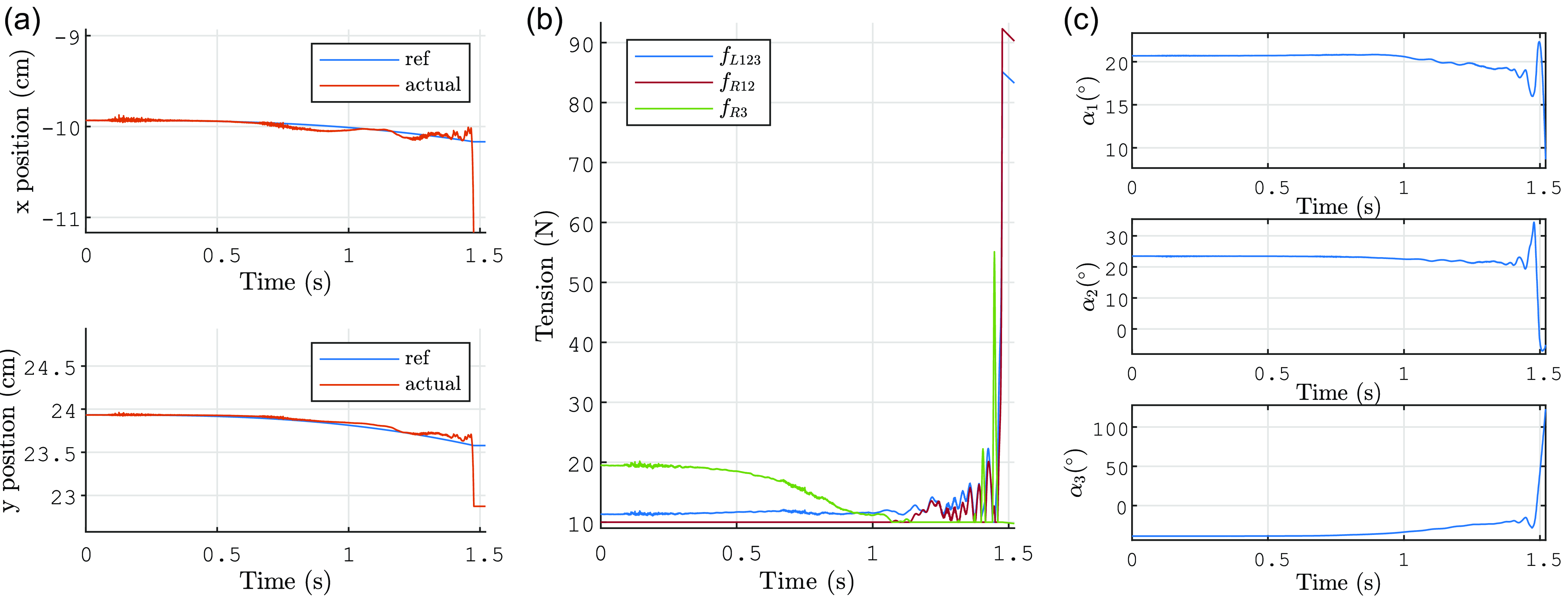
Figure 21 depicts the motion executed with the CTC from the configuration 1 to the configuration 3. Initially, the robot follows the desired EE trajectory but instability arises, leading to cable tensions reaching saturation. The robot configuration at which the CTC starts becoming unstable is marked by a green star in Figure 18. Notably, this configuration is not yet within the unstable zone on the graph. This discrepancy may be attributed to the influence of dynamic effects and friction, which were not considered in the stability analysis. Specifically, for the given joint angles $[\alpha _1,\alpha _3]^\top =[19.0^\circ, -15.1^\circ ]$ , the resulting angle $\alpha _2$ is observed to be $19.4^\circ$ , deviating from the expected $26.7^\circ$ calculated by static equilibrium. Consequently, the stability of the robot configurations is not accurately represented in Figure 18.

Figure 21.

Time histories of (a) $x$ and $y$ , (b) $\mathbf{f}$ , and (c) the $\alpha _i$ for the trajectory from configurations 1 to 3 from with the CTC. For (b), the plot colors correspond to the cable colors in Figure 17.

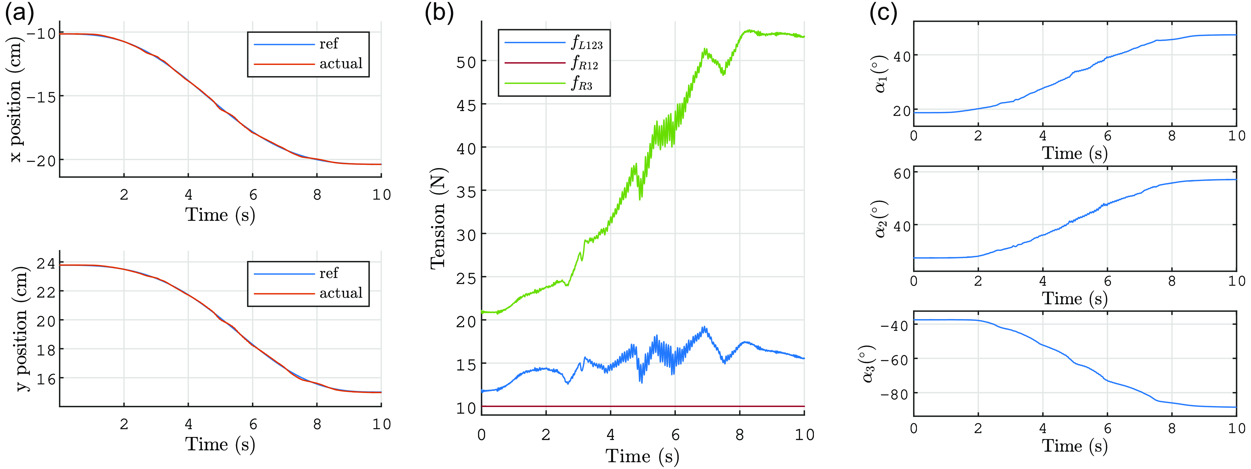
Figure 22 illustrates the same motion from configuration 1 to configuration 2 (with the same duration and PID tuning) executed with the PCTC. The control remains stable, similar to the CTC, and the curves exhibit a similar pattern. There are some differences in the oscillations of $\mathbf{f}$ due to friction effects, but the overall evolution is comparable. Additionally, the precision of the control is similar for both methods, with mean and maximum EE position errors of $4.0 \times 10^{-4}$ m and $2.0 \times 10^{-3}$ m, respectively, for the CTC, and $5.0 \times 10^{-4}$ m and $1.9 \times 10^{-3}$ m, respectively, for the PCTC.

Figure 22.

Time histories of (a) $x$ and $y$ , (b) $\mathbf{f}$ , and (c) the $\alpha _i$ for the trajectory from configurations 1 to 2 from with the PCTC. For (b), The plot colors correspond to the cable colors in Figure 17.

Figure 23.

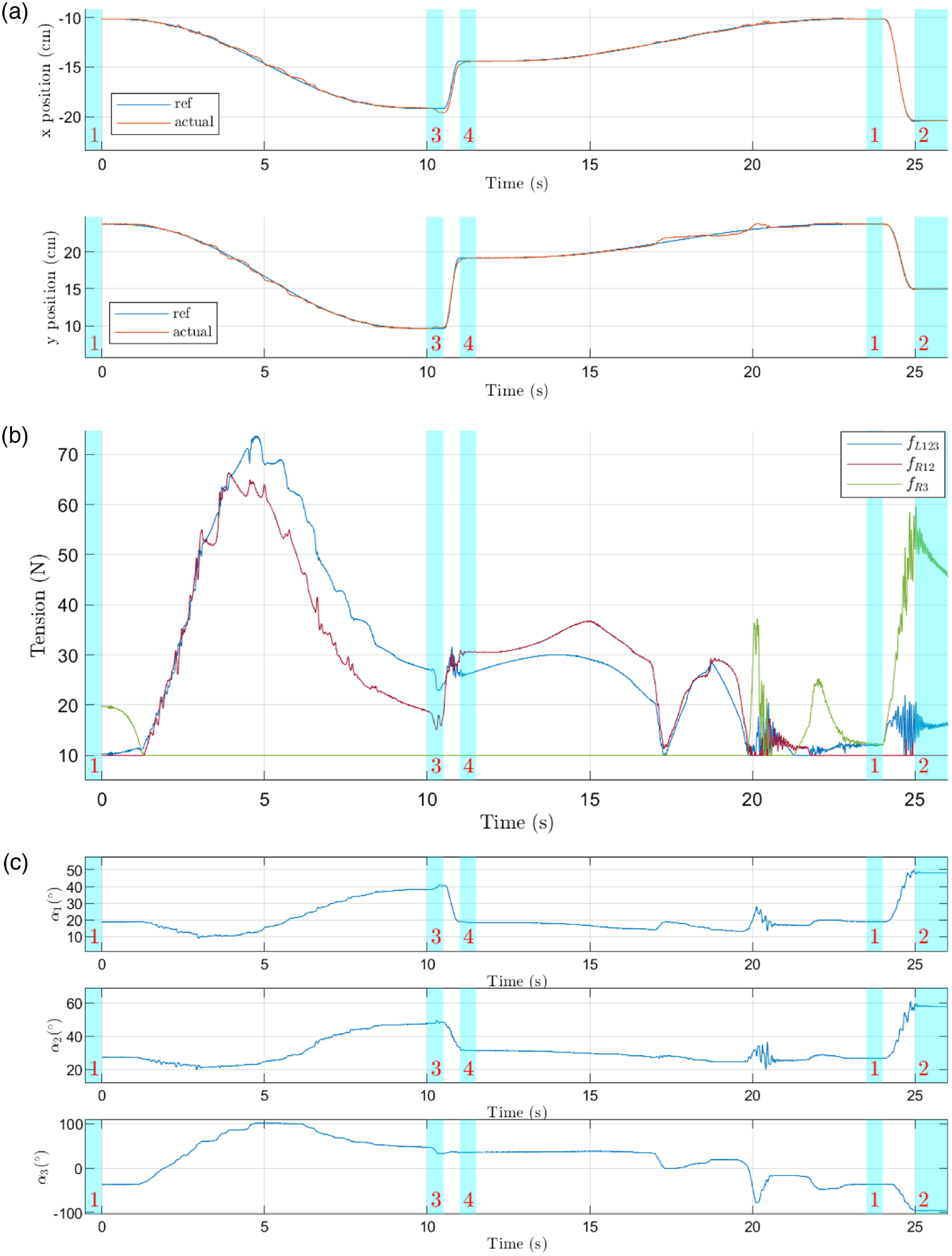
Time histories of (a) $x$ and $y$ , (b) $\mathbf{f}$ , and (c) the $\alpha _i$ for the trajectory from configurations 1 to 3, then to 4, then to 1, and finally to 2 with the PCTC. For (b), The plot colors correspond to the cable colors in Figure 17. The light blue areas indicate the desired numbered robot configurations of Figure 17.

We now design a motion that transitions from configurations 1 to 3 in 10 s, then to configuration 4 in 0.5 s, then back to configuration 1 in 12 s, followed by a transition to configuration 2 in 1 s, with a pause of 0.5 s between each trajectory. Figure 23 depicts the trajectory tracking with the PCTC. In line with the theoretical expectations, the control remains stable during the transition from configurations 1 to 3, in contrast to the CTC. The EE position tracking is generally good, albeit with some oscillations due to nonlinear friction. Notably, during the motion from configuration 4 to 1, friction-induced perturbations may cause abrupt changes in the robot configuration (see Figure 23 c). However, the control remains stable despite these disturbances. Additionally, Figure 23 a illustrates that the control remains effective during more rapid motions (from configurations 3 to 4 and from configurations 1 to 2).

These motions can be observed in the videos provided in the supplementary material.

5.3. Influence of an obstacle

Figure 24.

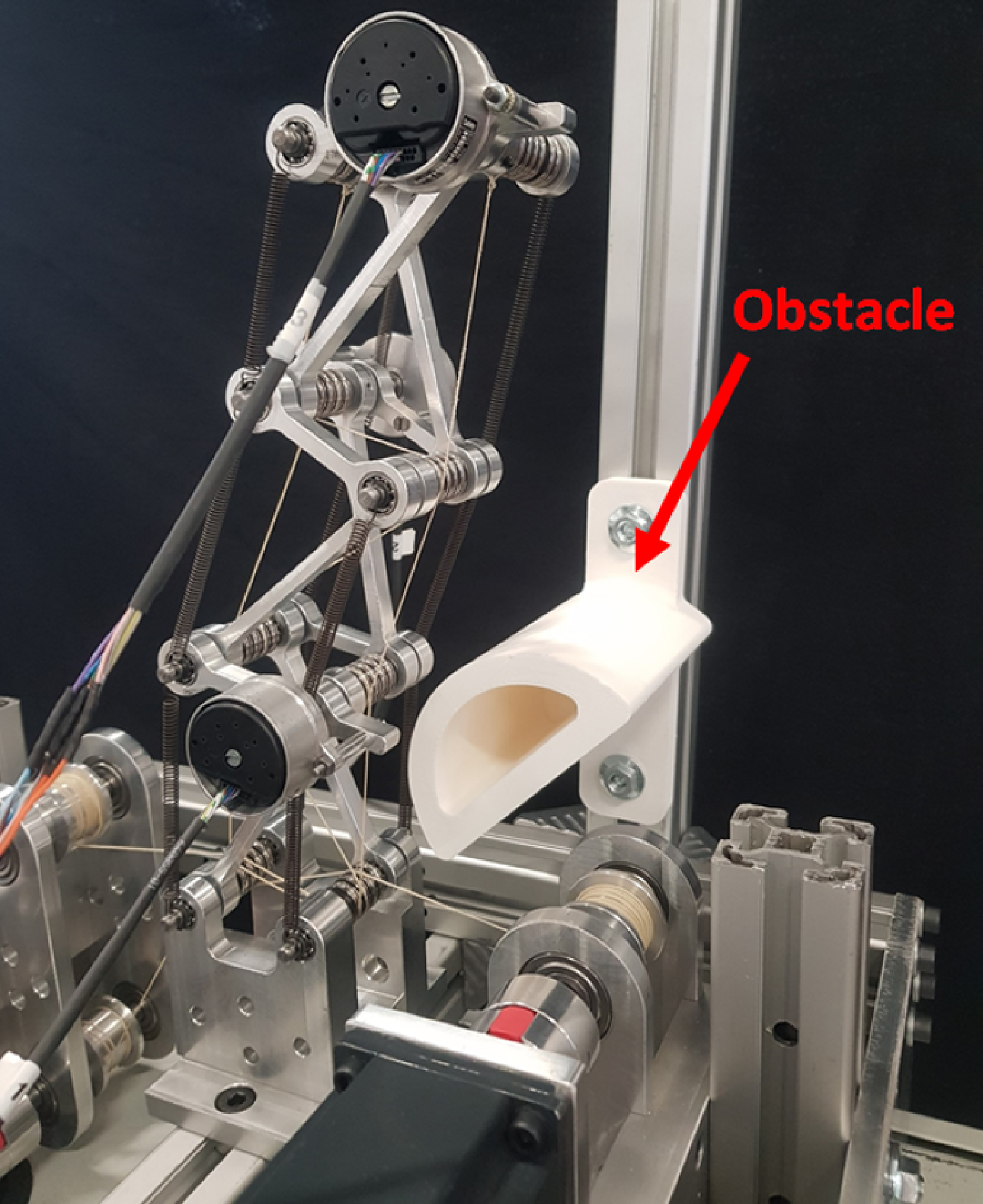
Prototype with an obstacle (picture from the back of the robot).

Figure 25.

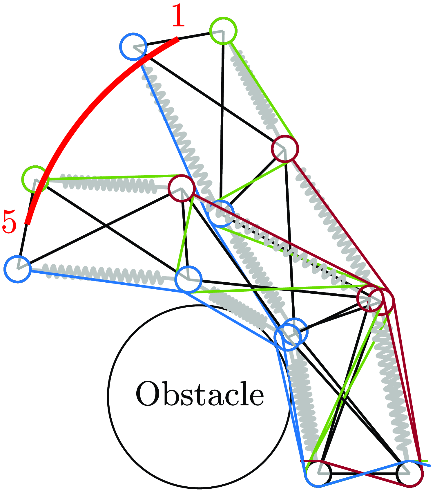
Desired trajectory from configuration 1 to configuration 5. In the latter, the robot is in contact with an obstacle.

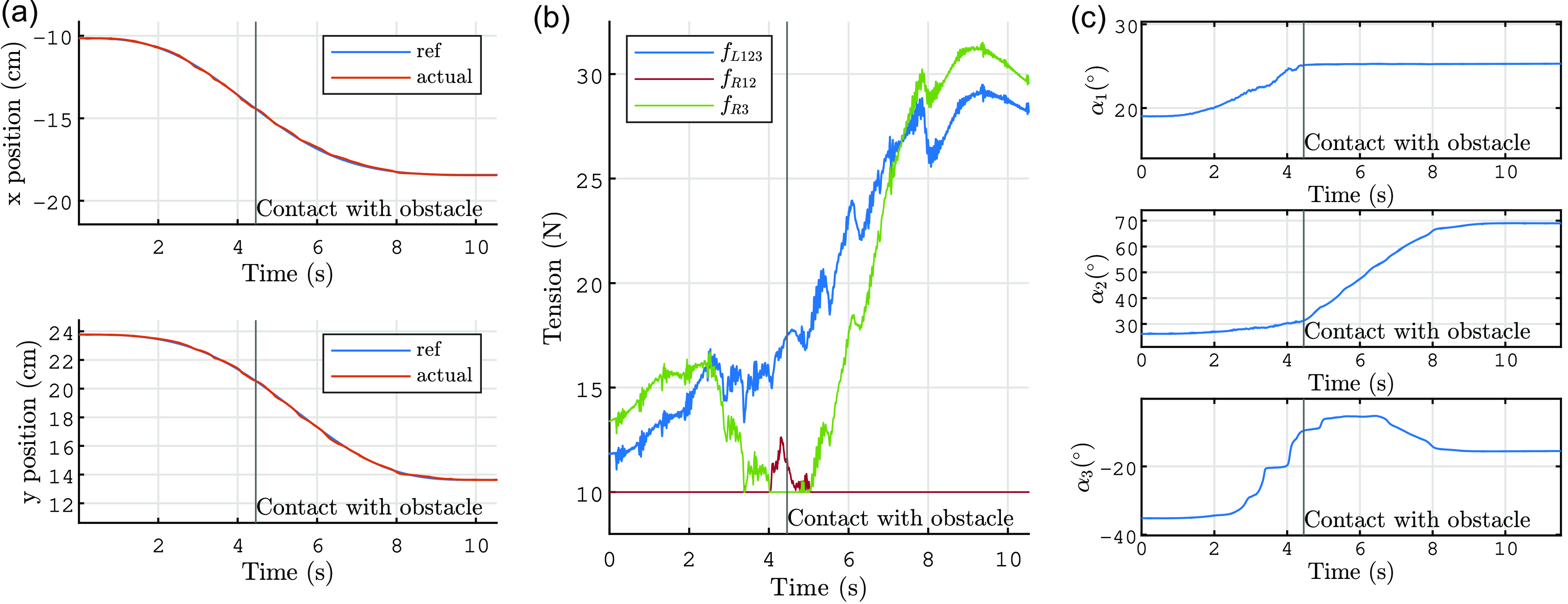
To further investigate the robustness of the control system, an obstacle has been introduced near the first joint, as depicted in Figure 24. A desired trajectory is illustrated in Figure 25. The outcomes of executing this trajectory in the presence of the obstacle are presented in Figure 26. Contrary to what Figure 25 suggests, the robot cables do not come into contact with the obstacles, as they are not in the same plane (refer to the video provided in the supplementary material). In Figure 26 c, it is evident that $\alpha _1$ ceases to evolve after 4.4 s due to contact with the obstacle. Despite this contact, the control remains stable post-4.4 s, even though the obstacle is not factored into the control algorithm. Notably, due to the freedom of joints 2 and 3, the trajectory tracking of the EE position continues unaffected (see Figure 26 a). Thus, we observe that underactuation enables the robot to naturally adapt to environmental contact.

Figure 26.

Time histories of (a) $x$ and $y$ , (b) $\mathbf{f}$ , and (c) the $\alpha _i$ for the trajectory from configuration 1 to 5 using the PCTC. For (b), The plot colors correspond to the cable colors in Figure 17. The vertical black line indicates when the robot enters in contact with the obstacle.