Implications
Our study shows that artificial insemination can be used successfully under tropical conditions. The results obtained have allowed us to estimate the first genetic parameters (heritability, heterosis and recombination loss) of this fertility trait in a large population of Holstein–Zebu cross-breed cows. The main result of our study is that there exists heterogeneous genetic (co)variance across the different proportions of Holstein–Zebu blood in the cows. The use of a random regression model allows us to identify the changes in genetic (co)variance and estimated breeding values in the whole trajectory of the different proportions of Bos taurus × Bos indicus blood.
Introduction
Artificial insemination (AI) is an essential tool for many cattle production systems and it is widely considered as a basic component in any cattle breeding programme (Van Arendonk, Reference van Arendonk2011). However, it is important to study the factors affecting the results of each insemination, particularly under tropical conditions, where AI is used to a lesser extent (Thibier and Wagner, Reference Thibier and Wagner2002). There are two main problems when dealing with results from AI. The first is defining a measure, which is generally done using the non-return rate (Vishwanath, Reference Vishwanath2003), and which can be interpreted as an adequate but insufficient indicator of true pregnancy rate, which should be measured by rectal palpation. Second, the fact that the results of each insemination depend on the fertility capacity of the cows and the sire, which means that these two elements must be included in the statistical model when analysing the variability of these traits.
Results from previous studies have indicated a low heritability in the fertility rate of AI sires (Menéndez-Buxadera and Rodriguez, Reference Menéndez-Buxadera and Rodriguez1996; Thaller, Reference Thaller1998; Averill et al., Reference Averill, Rekaya and Weigel2004; Weigel, Reference Weigel2004; Berry et al., Reference Berry, Evans and McParland2011), but the genetic coefficients of variation are around 15%. Given the fact that each sire performs thousands of inseminations each year, this allows us to carry out genetic evaluations and selection. The procedures for assessing this fertility trait have been proposed in Interbull (Thaller, Reference Thaller1998); nevertheless, it is essential to have a good population recording system, which is not always available, even in those countries where a comprehensive dairy control system is in place. For this reason, an indirect method of measuring fertility is used (Clay and McDaniel, Reference Clay and McDaniel2001; Kuhn et al., Reference Kuhn, Hutchison and Norman2008).
In Cuba, most of the female population included in the AI program are pure-bred Holstein (H) and Zebu (Z) cows, as well as some crosses between the two breeds. The AI results are measured by individual rectal palpation 60 to 90 days post-insemination, and the data are recorded by the National Recording Centre, which belongs to the Ministry of Agriculture. As a result, a large database is available that is currently being used to study the sources of variation in AI sires and insemination technicians. In addition, the characteristics of this data set could be of great use for animal breeding in the tropics, because they allow us to compare different statistical models in order to estimate genetic parameters and estimated breeding values (EBVs) accounting for cross-breeding effects in a cow population with different proportions of H and Z blood.
In terms of genetic evaluation in pure-bred and cross-bred animals, van der Werf, (Reference Van der Werf1990) recommended the incorporation of cross-breeding coefficients (additive, heterosis and recombination loss) as fixed covariables and the animal effect as a random variable to estimate the additive genetic variance component. In this non-additive model, it is implicitly assumed that the genetic (co)variance is the same throughout the whole range of the trajectory for the cows of different breed composition. However, this viewpoint can bias the results, as was recently shown by Hickey et al. (Reference Hickey, Calus, Cromie, Keane, Brophy and Verkamp2006) and Lidauer et al. (Reference Lidauer, Mantysaari, Strandén, Poso, Pedersen, Nielsen, Johansson, Ericksson, Madsen and Aumand2006), who obtained more accurate results in the genetic evaluation of cross-bred animals when the random genetic effect was estimated across the scale of cross-breeding coefficients.
The objective of this study was, first, to estimate the main factors affecting AI results under tropical conditions, and second, to estimate genetic (co)variance and EBV from the classical additive, non-additive and longitudinal sire models accounting for the different proportions of Holstein and Zebu breeds in the cows.
Material and methods
The results from a total of 1 345 000 inseminations, carried out in Cuba between 1994 and 2003, were available for this analysis. The editing process ensured that at least 25 inseminations for each sire, a minimum of 50 inseminations per AI technician and over 150 inseminations for each herd were represented. Finally, a total of 905 149 inseminations were used (167 453 in heifers and 737 696 in cows) from 815 sires and performed by 982 AI technicians in 3249 large herds throughout the country. The genotypes of AI sires (gs) were pure Holstein (H; n = 203), pure Zebu (Z; n = 206) and H × Z cross-breds (CB; n = 406; those of CB sires were 75H : 25Z; n = 113 and 62.5H : 37.5Z; n = 293). At least two types of gs and two breed compositions of the cows were represented in each herd. Table 1 shows the number of inseminations by H breed proportion of the cows and the genotype of the sire. The links between AI sires were guaranteed, as they were the product of different crosses between H and Z, and the pedigree was extended three generations back for a total of 1169 sires.
General information about total inseminations realized by type of cows and sires genotype

AI = artificial insemination.
aPercentage of Holstein breed in the inseminated cows.
Sire fertility (SF) was defined as 1 if the cow became pregnant after insemination and 0 if not. The diagnosis of pregnancy was carried out by rectal palpation 60 to 90 days after the insemination. In our procedure, the number of pregnant cows relative to the number of inseminations was equivalent to the mean SF, and these pooled quantities were recorded nationally by the National Recording Centre and used for a monthly estimation of SF for each sire as follows:
SF = (total number of pregnancies/total number of inseminations) × 100.
The individual identification of the cows was not recorded but the breed composition was known, and this information was used to estimate the importance of the cow effect by using their individual cross-breeding coefficient:
additive coefficients [add = 0.5 (pf + ps)];
heterosis coefficients [het = ps (1 − pf) + pf (1 − ps)];
recombination losses [rec = ps (1 − ps) + pf (1 − pf )].
In these cases, ps and pf refer to the proportion of Holstein blood of paternal and maternal origin for each cow, respectively. According to their cross-breeding coefficients, the genetic composition (gc) of the cows was grouped into six classes (Table 2). The same cross-breeding coefficients were estimated for each AI sire.
Genetic cross-breeding coefficients estimated for the genotype of the cows

aPercentage of Holstein breed in the cows.
bThe general mean for all data.
The available data were analysed by four different linear models, using ASReml (Gilmour et al., Reference Gilmour, Cullis, Welham and Thompson2000), which can be represented as follows:
 $${{y}_{ijklmn}}\:{\rm{ = }}\:fixe{{d}_i}\:{\rm{ + }}\:g{{s}_j}\:{\rm{ + }}\:g{{c}_k}\:{\rm{ + }}\:sir{{e}_l}\:{\rm{ + }}\:te{{c}_m}\:{\rm{ + }}\:re{{s}_{iijklmn}}$$
 $$no{{{y}_{ijklmn}}\: {\rm{ = }}\:fixe{{d}_i}\:{\rm{ + }}\:g{{s}_j}\:{\rm{ + }}\:{{b}_{1add:k}}\:{\rm{ + }}\:{{b}_{2het:k}}\:{\rm{ + }}\:{{b}_{3rec:k}}\:\cr \quad{\rm{ + }}\:sir{{e}_l}\:{\rm{ + }}\:te{{c}_m}\:{\rm{ + }}\:re{{s}_{ijklmn}} $$
 $${{y}_{ijklmn}}\:{\rm{ = }}\:fixe{{d}_i}\:{\rm{ + }}\:g{{s}_j}\:{\rm{ + }}\:sir{{e}_{lk}}\:{\rm{ + }}\:te{{c}_m}\:{\rm{ + }}\:re{{s}_{ijlmnk}}$$
 $$no{{{y}_{ijklmn}}\: {\rm{ = }}\:fixe{{d}_i}\:{\rm{ + }}\:g{{s}_j}\:{\rm{ + }}\:\mathop{\sum}\limits_{r\: = \:0}^2 {{{\beta }_k}{{\rPhi }_r}} \: + \:\mathop{\sum}\limits_{r\: = \:0}^2 {{{\alpha }_{j{\rm{:}}k}}{{\rPhi }_r}} \: \cr \quad+ \:te{{c}_m}\:{\rm{ + }}\:re{{s}_{ijlmn:k}} $$
In all these models, yijklmn is the vector of SF records; the fixedi parts include the effects of herds (3249 levels); years–months of insemination (116 levels); type of female (two levels, heifer or cow); gsj and gck represent the genotype groups of the sires (three levels) and the cows (six levels), respectively. In model A1, these two last fixed effects were included as a parent group effect in an additive sire model. Model A2 is a non-additive sire model, where b 1, b 2 and b 3 are a linear regression on the coefficients for additive (add), heterozygosity (het) and recombination loss (rec), which were included to account for the gck effect. The corresponding cross-breeding coefficients b 1, b 2 and b 3 belonging to gsj were also tested in model A2 but were not significant. Model A3 is a multi-trait additive sire model in which the results from each gck were considered as different traits. A random regression additive sire model was used in model A4, where the gck effect was modelled by a fixed regression coefficient (βk) to account for the fixed curve of response of SF along the scale of the additive cross-breeding coefficient of the population of cows. In Model A4, the αj :k is the random genetic regression and Φr is the Legendre polynomial coefficient or r order. In this random regression model (RRM), the permanent environmental effect was not included; however, this fact does not preclude the use of a random regression model at the sire level, because the genetic (co)variance of the dependent variable was estimated as a deviation of the fixed trajectory of different Holstein breed proportions in the cows. The same approach was used by Hickey et al. (Reference Hickey, Calus, Cromie, Keane, Brophy and Verkamp2006) and De Haas et al. (Reference De Haas, Janss and Kadarmideen2007).
For all the models, the random effects were: the sirel (1169 levels including AI sires with data and their ancestors without data); the AI technician (tecm with 982 levels) and residual effects; res was homogeneous for models A1 and A2 and heterogeneous with six classes (the same as gck) for models A3 and A4.
In matrix notations, all the models were very similar and can be represented by
 $$ {\bf y}\:{\rm{ = }}\:{\bf Xb}\:{\rm{ + }}\:{\bf Z}{{\bf S}_i}\:{\rm{ + }}\:{\bf W}{{\bf T}_j}\:{\rm{ + }}\:{\bf R} $$
where y is the vector of records, b are the fixed effects vectors, Si, Tj and R are the random effects of the sire, AI technician and residual, respectively. X, Z and W are the incidence matrices of fixed and random effects, respectively. For models A1, A2 and A3, it is assumed that first and second moments of the models are
 $${\bf E}({\bf y})\:{\rm{ = }}\:{\bf Xb} \ {\rm{and}} \ {\rm{var(}}{\bf y}{\rm{)}}\:{\rm{ = }}\:{\bf Z}{\rm{(}}{\bf G} \otimes {\bf A}{\rm{)}}{\bf Z}^{\prime}\:{\rm{ + }}\:{{\bf I}_i}\sigma _{t}^{2} \: + \:{\bf R}$$
For the RRM, A4 only changes in the first term in the expected variance:
 $${\rm{var(}}{\bf y}{\rm{)}}\:{\rm{ = }}\:{\rm{\rPhi (}}{{{\bf K}}_s} \otimes {\bf A}{\rm{)\rPhi }}^{\prime}\: + \:{{{\bf I}}_i}\sigma _{t}^{2} \: + \:{\bf R}$$
where I is the identity matrix of order equal to the number of tec with variance  $$$\sigma _{t}^{2} $$$; A is the additive genetic relationship matrix among sires; G is the genetic variance matrix for A1 and A2, although in Model A3, this G represents a 6 × 6 genetic (co)variance matrix for SF recorded in different gc; Ks is the genetic random regression coefficients matrix; R is the residual variance matrix and ⊗ is the direct product operator. The Z matrix has values of 1 or 0 for models A1, A2 and A3. Model 4 is an RRM in which the Z matrix contains the Legendre polynomial (Φr) coefficients on the scale of additive cross-breeding coefficients belonging to gck (see Table 2). Different orders of fitting in the RRM were compared according to the recommendations of Foulley and Robert-Granie (Reference Foulley and Robert-Granie2002). In all models, the dependent variable was weighted by the total number of inseminations.
The genetic (co)variance, genetic parameters and their standard error were estimated as a linear function of the corresponding components following the recommendation of Gilmour et al. (Reference Gilmour, Cullis, Welham and Thompson2000). In the case of the RRM, the genetic variance for the SF at point k of the trajectory of add coefficients of the cow were estimated following recommendations of Jamrozik and Schaeffer (Reference Jamrozik and Schaeffer1997):
 $$\sigma _{{{{S}_k}}}^{{\rm{2}}} \: = \:4({{\rPhi }_k}{{{\bf K}}_s}\rPhi _{{ k}^{^{\prime}} )$$
The genetic covariance between the SF results measured in the cows at points k 1 and k 2 of the trajectory of the add scale was estimated by
 $${{\sigma }_{{{k}_{{\rm{12}}}}}}\: = \:{{\rPhi }_{{{k}_{\rm{1}}}}}{{{\bf K}}_s}\rPhi _{{{{k}_{\rm{2}}}}}^{^{\prime}} $$
From these components, the h 2 and genetic correlation (Rg) are estimated using classic formulae and the corresponding residual variance. In this RRM procedure, the solutions for each sire are obtained for the r coefficients of random regression with which the EBV for the i th sire can be estimated for any k of additive coefficient of the cows, as follows:
 $${\rm{EBV}}_{k}^{i} \: = \:\mathop{\sum}\limits_{r\:{\rm{ = }}\:{\rm{0}}}^2 {{{\rPhi }_k}{\bf S}_{i}^{^{\prime}} } $$
where Si = r 0, r 1, r 2 represents the solution for the i th sire, given by the intercept (r 0), linear (r 1) and quadratic (r 2) genetic coefficients from a second order Legendre polynomial of kr. By using the Si solutions and the corresponding effect for gs and the Φk coefficients, the EBV of each AI sire can be estimated along the scale of additive coefficient of the cows.
Before this complex genetic analysis, several fixed linear models were also applied to the same data set. In this case, all the previously fixed effects were included in order to estimate different parameters to describe the response pattern of each factor affecting the SF.
Results
General results and environmental factors
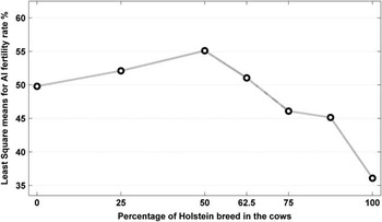
The least square means results of SF in the population studied are presented in Figure 1. The fertility level of cows with <50% H breed shows a highly significant rate of increase (P < 0.001), which thereafter decreases, until it reaches very low results for Holstein pure cows. During the first 7 years, the results of SF (Figure 2) showed a net increase from 26.1% in 1994 to 70.2% in 2000, thereafter decreasing to 47.1% in 2003 (48.8% for the whole period of time). The SF results were significantly better (P < 0.001) in heifers (+1.48% ± 0.26) compared with cows.
Least squares means for the success of AI in cows with different proportions of Holstein blood. AI = artificial insemination.

Least squares means for sire fertility during the period of time represented in the database.

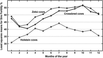
The monthly fertility pattern for females is presented in Figure 3. For simplicity, the results from cows with 25% H to 75% H were combined and expressed as cross-bred cows. The Zebu and cross-bred cows showed approximately the same pattern during all the months of the year, with a higher pregnancy rate than Holstein cows. In general, better fertility results were attained during the summer (June to September), whereas they were lower at the beginning and the end of the year. The percentage of total inseminations carried out was higher at the beginning and the end of the year (results not shown) and the three cow genotypes showed a similar pattern.
Least squares means results for sire fertility on a monthly basis in different types of cows.

The effect of the AI technicians was an important source of variation affecting the SF results and the solution of this random effect shows a variation coefficient was 9.6%.
Cross-breeding effect and genetic parameter results
Although the average cross-breeding coefficients of the sires and the inseminated females were very similar in terms of add and het components (see Table 2), the rec coefficients were twice as high in the three sire genotypes compared with females. The genetic composition of the sire changed from add = 0.61 to 0.57, het = 0.19 to 0.37 and rec = 0.19 to 0.34, for 1994 and 2003, respectively, whereas the genetic composition of the inseminated females changed from add = 0.68 to 0.52 and het = 0.15 to 0.53 during the same period. Although the gs effect estimated from Model A2 was not significant, the cross-breeding coefficient effect for gc was highly significant (P < 0.001; add = −3.02% ±0.59; het = 4.69% ± 2.1 and rec = −4.11% ± 2.1) in the inseminated cows.
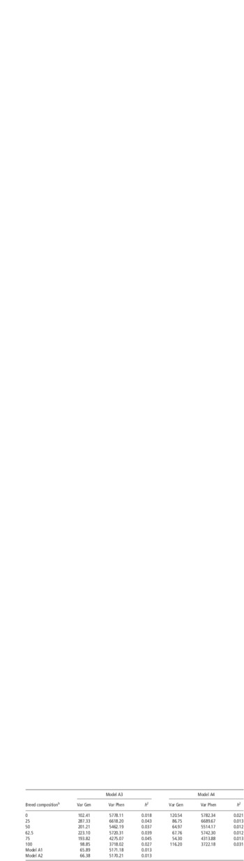
The use of the parent group effect, or the corresponding cross-breeding coefficients as fixed effects in models A1 and A2, had no effect on the genetic variance and heritability (h 2) of SF, which were the same in both models (h 2 = 0.013 ±0.001), with a genetic variation coefficient of 16.9%. However, the results of the multi-trait model (Model A3) show that the genetic variance and the h 2 values were not the same across the six genotypes of inseminated cows (Table 3), which is assumed in models A1 and A2. The residual variance was homogeneous in models A1 and A2, but heterogeneous with six classes (the same as gc) in models A3 and A4.
Heritability (h 2)a, genetic (Var Gen) and phenotypic (Var Phen) variance, for SF estimated by different model across the breed composition of the inseminated cows

SF = sire fertility.
aThe standard errors of h 2 were ±0.0012 for models A1 and A2; ±0.0028 to ±0.0030 for Model A3 and ±0.0032 to ±0.0039 for Model A4.
bPercentage of Holstein breed in the cows.
The genetic variance from Model A3 in the Zebu and Holstein cows (0% and 100% H breed composition, respectively, in Table 3) was very similar, although the residual variance in H was lower, and consequently, the h 2 was higher when SF was recorded in these pure-breed cows. The genetic variance and h 2 in cross-bred cows (breed composition between 25% to 75% H in Table 3) were generally higher than the same parameters estimated in H and Z pure-breed cows.
Legendre polynomials of different orders were compared in Model A4. An order 2 (quadratic) Legendre polynomial showed the best overall suitability compared with Legendre polynomials of order 1 (linear) and order 3 (cubic) on the basis of log L, Akaike information criterion (AIC) and Bayesian information criterion (BIC) model comparison criteria. The resulting Ks matrix of this A4 model and the Φk coefficients were used to estimate the genetic variance and h 2 across the whole range of the females breed proportion and these results are also presented in Table 3. The A4 model shows more homogenous results compared with the same parameters from the multi-trait A3 model.
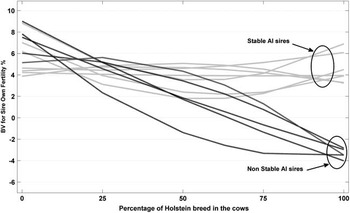
The genetic correlations between SF recorded in females with different breed composition and estimated from models A3 and A4 are presented in Table 4. For both models, it was evident that SF recorded in different female breed types cannot be considered as the same trait. For females with a similar breed composition (a difference of no more than 50% in add components), there is a high genetic correlation, which decreases to almost zero for cows with add = 0 (i.e. Zebu cows) and those over 50% in add components. The eigenvalues (λ) of the additive genetic correlation matrix show that the first and second λ accounted for 61.9% and 19.8% in Model A3 and 64.3% and 27.2% in Model A4 of the total genetic variation, respectively. According to Kirkpatrick et al. (Reference Kirkpatrick, Lofsvold and Bulmer1990), the associated eigenfunction for these λ can be used to evaluate possible deformation of the overall mean genetic trajectory of SF across the scale of breed composition of the inseminated cows. These can also be calculated using the results from RRMs (van der Werf and Schaeffer, Reference van der Werf and Schaeffer1997). Following the latter approach, the top 50 sires with more than 500 total inseminations were selected on the basis of their EBV results where the females have 0% of additive coefficients (Zebu cows). The trajectory of the EBV of these selected sires was estimated across the scale of breed composition of the cows, on the basis of the results of RRM Model A4, and the variability of SF EBV is presented in Figure 4.
Genetic correlationa for SF recorded on different breed composition of the cow and estimated for Model A3 (below diagonal) and Model A4 (above diagonal)

SF = sire fertility.
a***P < 0.001; **P < 0.01; *P < 0.05 and ns (P > 0.05).
bPercentage of Holstein breed in the cows.
Evolution of the estimated BVs for sire fertility recorded in cows with different proportion of Holstein breed. BV = breeding value; AI = artificial insemination.

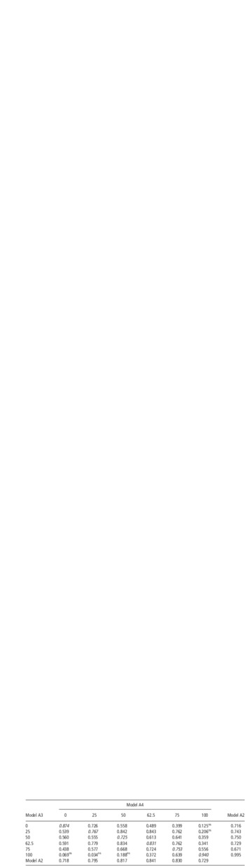
The correlation between EBV of the sires (weighted by its accuracy) estimated by A2, A3 and A4 models was estimated by including only those sires with more than 300 total inseminations (570 from the 1169 represented) and these results are presented in Table 5. The results from Model A1 are not shown because they were similar to those from Model A2. All the correlations were highly significant (except those indicated in Table 5), but lower than unity, with the exception being models A3 and A4, when SF was recorded in pure Zebu or pure Holstein cows. If the results from the three models are compared within the breed composition of the cows, the EBV from models A3 and A4 are more correlated than the results from model A2 (Table 5).
Correlationa between EBV for SF, estimated by three models and different breed composition of the cowb (570 AI sires with at least 300 total inseminations)

EBV = estimated breeding value; SF = sire fertility; AI = artificial insemination.
aAll correlations were highly significant (P < 0.001) except those with ns (P > 0.05).
bAs additive genetic coefficients in Model A4 and as genotype of the cows in Model A3.
Discussion
Our study shows that AI can be used successfully under tropical conditions. The results from different Holstein–Zebu cross-bred cows were very satisfactory, and were similar to those of native cows and to the first study published in Cuba with this type of pure- and cross-bred cow population (Menéndez-Buxadera et al., Reference Menéndez-Buxadera, Morales, Dora, Iglesias and Chávez1976). Considering the results of the monthly fertility pattern, together with our unpublished results on the effects of calving month on milk production, the option of concentrating calving in a shorter period of the year deserves greater attention, as it can provide important economic benefits under these tropical conditions.
The het level obtained in this study is equivalent to 9.6% of the mean SF; however, most of this beneficial effect is lost because the rec was −8.4%. The literature on this subject shows a high level of heterosis in fertility traits, particularly in the case of Bos taurus × Bos indicus crosses. In the review by Cunningham and Syrstad (Reference Cunningham and Syrstad1987), het was around 7% for the calving interval, and more recent papers by Mackinnon et al. (Reference Mackinnon, Thorpe and Baker1996), Kahi et al. (Reference Kahi, Thorpe, Nitter and Baker2000) and Demeke et al. (Reference Demeke, Neser and Schofman2004) show the same level of heterosis. Interestingly, in the latter three studies, the estimation of recombination loss tended to be as high as the het. The same results were presented by Wall et al. (Reference Wall, Brotherstone, Kearney, Woolliams and Coffey2005), for the non-return rate as a trait of cows, using a large Holstein–Friesian data set from the United Kingdom. Although these other studies involve different fertility traits, the results for SF coincide with these trends.
The variability between results from AI technicians was very important and accounted for <0.7% of the total phenotypic variance, which was similar to the results of Berry et al. (Reference Berry, Evans and McParland2011). However, in the Cuban animal production system, with extremely large, centralized herds, the tec results must be closely and continuously controlled, as this collateral effect represents a very important factor affecting the global herd economy (Menéndez-Buxadera et al., Reference Menéndez-Buxadera, Caunedo Sibori and Fernández Santibañez2004).
On applying an additive or non-additive model, the h 2 estimates of a single insemination were relatively low in agreement with other recent studies on this trait (Averill et al., Reference Averill, Rekaya and Weigel2004; Weigel, Reference Weigel2004; Berry et al., Reference Berry, Evans and McParland2011). However, the genetic variation coefficient was around 17%, indicating that there is scope for improvement by means of selection. Although the genetic (co)variance components and heritability from models A3 and A4 represent estimates of the same character, their interpretation is different. In the Model A3, these parameters correspond to total genetic components, whereas in A4, they refer to only the additive genetic components, and therefore the differences between both models are to be expected.
The genetic correlations (Rg) between SF measured across the breed composition of the cow are lower than unity, which implies that they are not the same trait. The highest levels of Rg were found between cows with no more than 50% difference in their breed composition. This is the first evidence published in tropical conditions that suggests that results from pure- and cross-bred animals are different but genetically correlated traits. This result will be of great importance in breeding programmes in the tropics, where animals with different proportions of taurus–indicus blood are very common.
There has been increasing interest recently in the genetic analysis of pure- and cross-bred populations. Studies published by Elzo and Bradford (Reference Elzo and Bradford1985) and Elzo and Famula (Reference Elzo and Famula1985) proposed a complex procedure for the overall evaluation of pure-bred and cross-bred animals, which was successfully used for the evaluation of B. taurus × B. indicus beef animals (Elzo et al., Reference Elzo, Manrique, Ossa and Acosta1998). More recently, Hickey et al. (Reference Hickey, Calus, Cromie, Keane, Brophy and Verkamp2006) proposed a more general procedure for multi-breed genetic evaluation, through the use of a RRM similar to that used in this study.
The relevant literature for predicting BVs of pure-bred and cross-bred animals shows that these correlations are high, but lower than unity (Elzo et al., Reference Elzo, Manrique, Ossa and Acosta1998; Newman et al., Reference Newman, Reverter and Johnston2002; Hickey et al., Reference Hickey, Calus, Cromie, Keane, Brophy and Verkamp2006; Menéndez-Buxadera and Mandonnet, Reference Menéndez-Buxadera and Mandonnet2006) for growth, milk production and carcass traits, respectively. Our results for SF agree with this trend only when the difference in genetic composition between inseminated cows is no more than 50% in additive genetic components. According to Wei (Reference Wei1992), this is the expected result when the genetic distances between the genotypes are very large, as in the case of B. taurus and B. indicus.
Two major implications emerge from our results for animal breeding programmes in the tropics. The first is that the assumption of the same genetic (co)variance and EBV across the percentage scale of Holstein breed in the cows is not completely valid for this type of the cross-breeding, and therefore the results from a classic statistical procedure for estimating BVs need to be changed and adapted to the structure of breed proportion in this type of population. However, such a strategy is not so easy to apply in the tropics where the recording systems are not very well developed.
The second problem is linked to the genetic interpretation of the genetic correlation matrix. According to the eigenvalue decomposition of this matrix, two types of response are expected across the breed composition of the cows, and the EBV response pattern presented in Figure 4 confirm this expected results. Those sires with a stable or a non-stable EBV across the breed composition of the cows are those related to the corresponding coefficients for the first eigenvector (known as a vector of size) and the second eigenvector (known as vector of form), respectively. The stable group can be defined as sires with an extremely important general combining ability (GCA) and the non-stable group would include those with a specific combining ability (SCA). It should be pointed out that these results were estimated with high level of accuracy, because there were 2340 and 3752 total inseminations for each sire for stable and non-stable groups, respectively. In genetic terms, GCA is largely due to additive gene effects, whereas SCA is a deviation due to dominant and epistasis gene effects. According to the excellent meta-analysis published by Rutledge (Reference Rutledge2001), these two last genetic effects are the reasons why attempts to obtain a tropically adapted dairy breed from taurus–Zebu crosses failed during the last century. Our results, obtained from a RRM, show that this procedure could be extremely useful for tropical animal breeding in order to identify and select suitable sires (those with higher GCA), and therefore enable us to carry out our work more efficiently.
With regard to the statistical model used in this study, the trait SF was expressed by the ratio of the sum of the pregnant and non-pregnant cows, compared with the total number of inseminations. With the use of pooled data, it took less time to construct the system of equations for the mixed model, as compared with a threshold model, thus saving computing time and resources. Our procedure was based on the one originally proposed by Olson et al. (Reference Olson, Garrick and Enns2006) and applied successfully by Biscarini et al. (Reference Biscarini, Bovenhuis and van Arendonk2008), Biscarini et al. (Reference Biscarini, Bovenhuis, Ellen, Addo and van Arendonk2010) and Cooper et al. (Reference Cooper, Ferrell, Cundiff and Van Vleck2010), where the original variables were pooled and the average performance was treated as if it pertained to each individual in the pool.
Conclusion
Our study shows that AI can be used successfully under tropical conditions. Very important and beneficial effects were estimated for heterosis (+9.6% of the mean), but the recombination loss proved to be just as high. Although the heritability of a single insemination was very low, the genetic variation coefficient was over 15%, which means that this source of variation can be used. Although more work needs to be done on the use of a RRM for genetic evaluation for different economical traits under tropical conditions, this statistical approach is highly recommended for the breeding process, because it allows us to identify the changes in genetic variance and in BVs over the whole range of different proportions of B. taurus × B. indicus blood.
Acknowledgements
The authors thank Dr Raphael Mrode, editor of Breeding & Genetics, and the two anonymous reviewers for their kind assistance.