INTRODUCTION
Variations in sediment color resulting from physical and/or biogeochemical processes provide important data to reconstruct paleoenvironmental change. These applications are wide ranging and include the (1) identification of paleosols (Kemp et al., Reference Kemp, Whiteman and Rose1993; Yang and Ding, Reference Yang and Ding2003); (2) characterization of laminated sediments (Johnson and Ståhl, Reference Johnson and Ståhl2010; Weber et al., Reference Weber, Tougiannidis, Kleineder, Bertram, Ricken, Rolf, Reinsch and Antoniadis2010); (3) distinction between terrigenous and biogenic inputs in deep-sea sedimentary archives (Wilson and Austin, Reference Wilson, Austin, Dowdeswell and Ó Cofaigh2002; Hodell et al., Reference Hodell, Crowhurst, Skinner, Tzedakis, Margari, Channell, Kamenov, Maclachlan and Rothwell2013) used to infer paleoclimatic regimes (Itambi et al., Reference Itambi, von Dobeneck, Mulitza, Bickert and Heslop2009); and (4) determination of mineralogical composition, most notably the occurrence (Helmke et al., Reference Helmke, Schulz and Bauch2002; Ji et al., Reference Ji, Chen, Balsam, Lu, Sun and Xu2004) or diagenetic transformation of iron oxides (Schwertmann, Reference Schwertmann1971) and other redox-sensitive elements, such as manganese (Löwemark et al., Reference Löwemark, Jakobsson, Mörth and Backman2008), which impart color to sediments.
Traditionally, a Munsell color chart is used for color descriptions of terrestrial sedimentary archives (Boston et al., Reference Boston, Evans and Ó Cofaigh2010; Buggle et al., Reference Buggle, Hambach, Müller, Zöller, Marković and Glaser2014) because of its ease of use in the field and laboratory (Gale and Hoare, Reference Gale and Hoare2011). However, this method has several weaknesses. First, there are a limited number of color swatches against which to compare a sample. In addition, Munsell readings taken at different times on the same archive may vary between operators as the human eye perceives color differently depending on ambient light conditions and sediment water content, which also vary over time (Balsam et al., Reference Balsam, Deaton and Damuth1998). A second limitation is that sampling resolutions are low and the data are difficult to represent graphically. A more effective method of color characterization is the CIELAB (Commission Internationale de l'Eclairage) color space, which quantifies sediment color using reflectance, measured either directly on the sediment using a spectrophotometer (Balsam et al., Reference Balsam, Deaton and Damuth1999; Ding et al., Reference Ding, Ranov, Yang, Finaev, Han and Wang2002; Debret et al., Reference Debret, Sebag, Desmet, Balsam, Copard, Mourier and Susperrigui2011) or indirectly from high-resolution, line-scan digital images (Morellón et al., Reference Morellón, Anselmetti, Ariztegui, Brushulli, Sinopoli, Wagner, Sadori, Gilli and Pambuku2016). Although color reflectance logging is routinely applied to deep-sea sediment cores (Helmke et al., Reference Helmke, Schulz and Bauch2002; Hodell et al., Reference Hodell, Crowhurst, Skinner, Tzedakis, Margari, Channell, Kamenov, Maclachlan and Rothwell2013), its application to terrestrial sediments is underused.
In terrestrial environments, photographs provide an important archive of paleoenvironmental data, particularly where core sections or field exposures are no longer available, or where sediments have degraded. Potential applications of this data are wide ranging and at a variety of scales. At the local scale, examples include tracking changes over time of lithologic units and their sedimentary parameters, as exposed by the recession of open-face field sections by quarrying or the recession of cliff/riverbank sections by erosion. This could be upscaled to augment and improve, for example, the resolution of regional lithostratigraphic models, especially where field data are currently lacking. Alternatively, data collected from disparate field sections could be spliced together to produce a composite depth or time series. Even though the digitization of archive photographs for color/grayscale analyses is not new (summarized in Balsam et al., Reference Balsam, Deaton and Damuth1999), few studies have logged color reflectance data from digital images of present-day field sections and compared them against laboratory data. Hitherto, such experiments have been undertaken only on loess (Porter, Reference Porter2000; Zeeden et al., Reference Zeeden, Krauß, Kels and Lehmkuhl2017).
The present study investigates three research questions: (1) How valid are such comparisons when applied to other Pleistocene sedimentary sequences? (2) How well correlated are high-resolution reflectance data derived from different imaging techniques on the same sediment? (3) To what extent can reflectance data derived from a freshly exposed field section or sediment core be correlated with chronologically constrained sediments from the same site but which are no longer available? To address these questions we use color reflectance data determined on glaciolacustrine, loessic, and marine sediments. Our objectives are to (1) compare the data derived using over-the-counter digital cameras and line-scan imagery and (2) analyze the extent to which the reflectance patterns are linearly replicated using cross-correlation analysis.
FIELD SITES AND SEDIMENTS
The data analyzed in this investigation were determined from archive sediments collected over the previous 15 yrs. The example field sections, and any associated photographs, were chosen because they displayed characteristics—such as uneven surfaces or differential lighting—that might be typically encountered in archive photographs of terrestrial sediments.
Glaciolacustrine sediments
These sediments comprise laminated to faintly stratified silty clays, interbedded with silty sands (Murton, Reference Murton2017). Data were collected from two sites in the Vale of York, UK, a sedimentary basin infilled with up to 24 m of superficial deposits (Gaunt, Reference Gaunt1994; Ford et al., Reference Ford, Cooper, Price, Gibson, Pharoah and Kessler2008). Hemingbrough (53°52′N, 00°17′W) is the type site for these deposits (Thomas, Reference Thomas and Bowen1999), the uppermost 10 m of which is exposed here in a working quarry. Overlapping monoliths and photographs were taken of the section in July 2004. Our second site is Balkholme Common (53°44′N, 00°48′W), 12.3 km southeast of Hemingbrough, where a core was drilled to bedrock in June 2014.
Loess
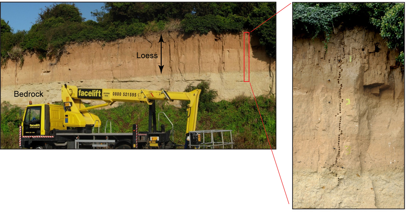
These eolian sediments are exposed in a sea cliff at Pegwell Bay, Kent, UK (51°19′N, 01°22′E), where they unconformably overlie Paleocene sand (Thanet Formation) (Murton and Giles, Reference Murton and Giles2016). Digital photographs were taken of the 3.5-m-thick eolian sequence (Fig. 1) in 2009, with three overlapping cores drilled to bedrock, 45 m west of this site, in 2010 and 2017.
Eolian sediments exposed in a cliff section at Pegwell Bay (left). Red box denotes sampling site, enlarged at right where depths are marked at 1 m intervals. Photographs courtesy of Julian Murton. (For interpretation of the references to color in this figure legend, the reader is referred to the web version of this article.)

Marine sediments
These sediments comprise greenish-grey hemipelagic nannofossil muds, with varying proportions of biogenic carbonate and terrigenous sediment (Expedition 339 Scientists, Reference Stow, Hernández-Molina and Alvarez Zarikian2013; Channell et al., Reference Channell, Hodell, Crowhurst, Skinner and Muscheler2018). Data were collected from two deep-sea cores drilled off the Iberian Margin in the North Atlantic Ocean: IODP U1385 (37°34′N, 10°7′W) and JC089 SHAK-06-4K (37°33′N, 10°8′W), cored in December 2011 and August 2013, respectively. The uppermost 6.00 m from core U1385D-1H (Supplementary Fig. 1) was used for our cross correlations as we considered this to be of sufficient length to compare with the 4.77-m-long SHAK06-4K core (Supplementary Fig. 2).
METHODS
Field sampling
At Hemingbrough, stepped trenches were cut mechanically into the 10 m open-face exposure, and the depths determined using an engineer's level and staff. Before photographing, each trench section was cleaned with a spade to produce a relatively even face. However, the cohesiveness of the moist sediments meant sedimentary structures, such as laminations, were often obscured by smearing. For laboratory analysis, samples were collected using overlapping 0.5-m-long plastic monoliths. For the purposes of this investigation, we focus on a 1.62-m-high section, where analog photographs had been taken of the laminated sediments (Fig. 2). At Balkholme Common, sonic drilling was used to collect a 13.7-m-long, near-continuous core in 1.55-m-length sections. The upper 4.5 m are incomplete owing to core loss, and are excluded from our analyses.
Field section of a dug trench at Hemingbrough showing the location of four overlapping monoliths and region of interest (yellow box) from which the standard image reflectance data were derived. Line-scan images of the four monoliths are shown to the right of the field section photograph. Blue arrow is at 7.5 m depth. (For interpretation of the references to color in this figure legend, the reader is referred to the web version of this article.)

At Pegwell Bay, the cliff face section was accessed from a cherry picker (Fig. 1). The top 0.4 m of the section was obscured by overhanging vegetation. The vertical sediment face was not cleaned, and depths were spray painted onto it at 1 m intervals. Cores were drilled by percussion.
Digital image preparation and acquisition
As recommended by Zeeden et al. (Reference Zeeden, Krauß, Kels and Lehmkuhl2017), any photographs used for digital image analysis should (1) have equal light exposure with no shadows, (2) be nondistorted and of a relatively high resolution, and (3) have no discernible differences in moisture content. Although these considerations are important, and certainly should be incorporated into future image analysis experiments, they cannot be applied retrospectively. Consequently, the photographs used in this investigation reflect the prevailing environmental conditions at the time, as might be typically encountered in archive photographs.
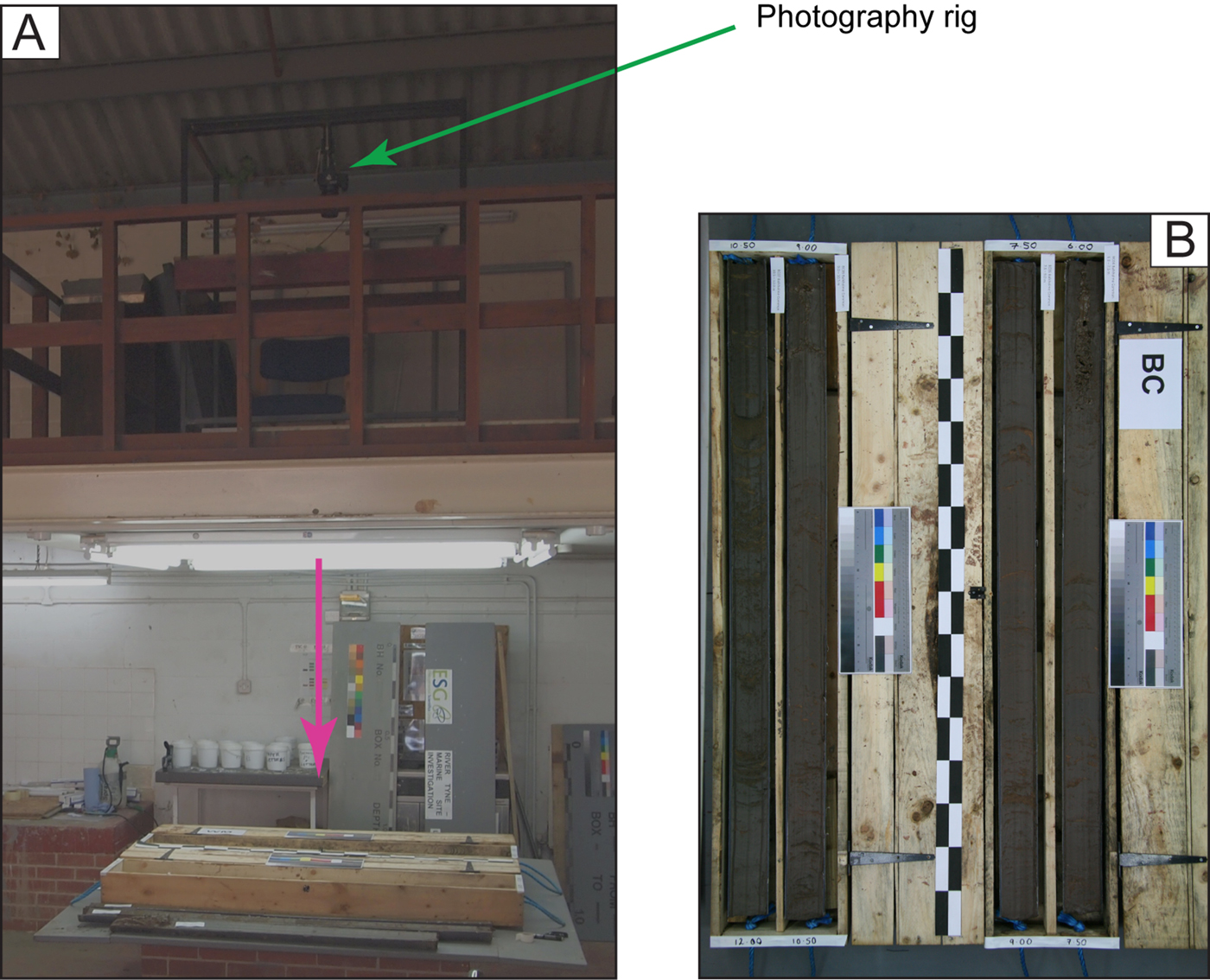
We used two digital imaging techniques. The first—termed the standard images herein—used over-the-counter digital cameras. This data set comprises the terrestrial sediments, including the analog Hemingbrough photographs subsequently digitized using an Epson line scanner. Ambient lighting during photography varied considerably. The field-based photographs from Hemingbrough and Pegwell Bay were obtained under sunny and cloudy skies, respectively. The Balkholme Common cores were split and imaged in a core-cutting workshop. In this environment, the uncleaned core sections were illuminated by eight fluorescent strip lights and imaged within an hour of splitting using a mounted digital camera (Fig. 3). No color or contrast adjustments were undertaken using software such as Adobe Photoshop.
(A) Photography rig setup for the standard images of the Balkholme Common sediments. The pink arrow indicates the central line of view. (B) Plan view of the raw photographs. Core length is 1.55 m, and the checked black and white ruler is in 10 cm increments. (For interpretation of the references to color in this figure legend, the reader is referred to the web version of this article.)

The second set of images—termed the line-scan images herein—was obtained using a Jai 3CCD high-speed color line-scan camera (model CV-L107) and linear light source integrated within an Avaatech XRF core scanner. This data set comprises the two Iberian Margin cores, Hemingbrough monoliths, and Balkholme Common and Pegwell Bay cores. The Iberian Margin cores were split, securely wrapped in cling film, and stored under refrigerated conditions (4°C) before being imaged several months later. The surface sediments had oxidized during this time. The laboratory procedure was identical for all cores. First, the working half was cleaned using a steel scraper drawn perpendicular to the sediment long axis. For imaging, a blackout blind was drawn over the scanner's observation window, ensuring the core sections were illuminated only by the integrated light source. The scan rate was 10 mm/s.
CIELAB color reflectance data logging
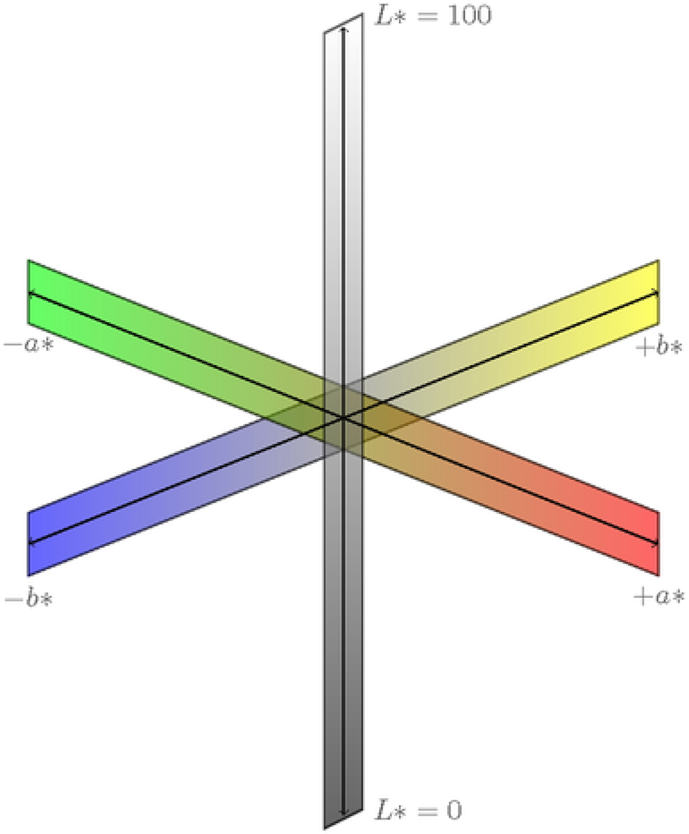
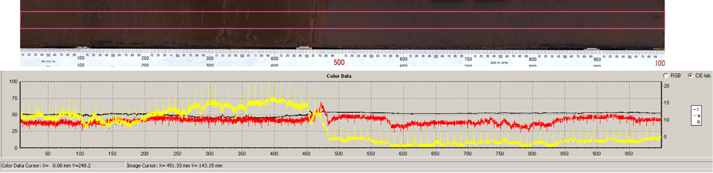
In the CIELAB color space, L* corresponds to lightness (or grayscale), whereas a* and b* relate to red–green chromaticity and yellow–blue chromaticity, respectively. Values are dimensionless and range for L* from 0 (black) to 100 (white), for a* from + 60 (red) to −60 (green), and for b* from + 60 (yellow) to −60 (blue) (Fig. 4). The field section standard images were cropped in IrfanView to remove extraneous detail. For all images, CIELAB color reflectance data were captured by uploading them into the Avaatech's image processing software and highlighting a region of interest (Figs. 2 and 5; Supplementary Figs. 1–4). The imaging software assigns zero—that is 0 μm—to the top of the image regardless of whether the image is of sediment or not. This is important for the standard images where, unlike the line-scan images, the ratio of pixel to sediment varies because of distortion effects. This is most pronounced at the edges of standard images. To account for this, reflectance data were also captured from the checked black and white ruler and staff respectively in the Balkholme Common and Hemingbrough standard images. These issues are discussed in the following section.
(color online) CIELAB (Commission Internationale de l'Eclairage) color space (downloaded from http://www.texample.net/media/tikz/examples/PNG/cielab.png).

Core section CIELAB (Commission Internationale de l'Eclairage) color data captured at 70 µm resolution from a highlighted (pink box) region of interest. The black, red, and yellow lines correspond to L*, a*, and b* reflectance, respectively. The orthogonal, regularly spaced lines extending from the a* and b* reflectance data are software-inserted artifacts, removed during data processing. Scale on x-axis is in millimeters and matches the ruler scale. A lithologic boundary at 480 mm is identified by a sharp decrease in b* reflectance values. (For interpretation of the references to color in this figure legend, the reader is referred to the web version of this article.)

Post-data-processing
Several post-data-processing routines were performed to ensure consistency between the data sets. First, the raw reflectance data were overlain—using Adobe Illustrator—on their respective image, and erroneous data points deleted. Such data may result from edge effects or minor sediment cracks. The raw reflectance data signal was reduced by applying a nonoverlapping 10 point moving average, except for the Pegwell Bay standard image data, which had significantly fewer data points than all the other data sets. These reduced data sets were used for the cross correlations.
Additional data processing routines were undertaken to counter nonlinear distortion and scaling differences in the standard images, as these can introduce errors into the depth scale. In these images, nonlinear distortion introduces a sediment stretching effect at points farthest from the camera lens, where the working distance is greater. The effect is more profound in the Hemingbrough field section, where the staff is inclined against an uneven sediment face. To correct for these distortions, we used reflectance data captured from the checked rulers (Balkholme Common) and staff (Hemingbrough) to determine the line-scan imaging depths corresponding to each increment. These data were input into the Poly2 mathematical routine in MATLAB to solve for the best polynomial fit. No distortion correction was applied to the Pegwell Bay data as the one meter depth intervals were only approximately marked.
Scaling refers to the ratio between an image pixel and the length of sediment to which it equates. For the highest data resolution, we require the highest ratio possible of pixels to distance. The Avaatech imaging software captures reflectance data at a resolution of 70 µm at the standard sample-to-camera distance. What is critical for this investigation is the scaling ratio, which differs between the two data sets. For the line-scan images, where the scaling factor is consistent and incorporated into the imaging software, 1 pixel always equates to 70 µm of sediment; therefore, the sample depth (e.g., 12.007 mm) recorded by the imaging software corresponds to actual depth (e.g., 12.007 mm) (Fig. 5). However, for the standard images, where the resolution is considerably lower, 1 pixel corresponds to more than 70 µm of sediment. In these images, where the real depth of our field or core section is known—from the core liner length or staff—we multiply by a scaling constant to convert the line-scan sampling depths to actual depths.
Pegwell Bay composite reflectance data
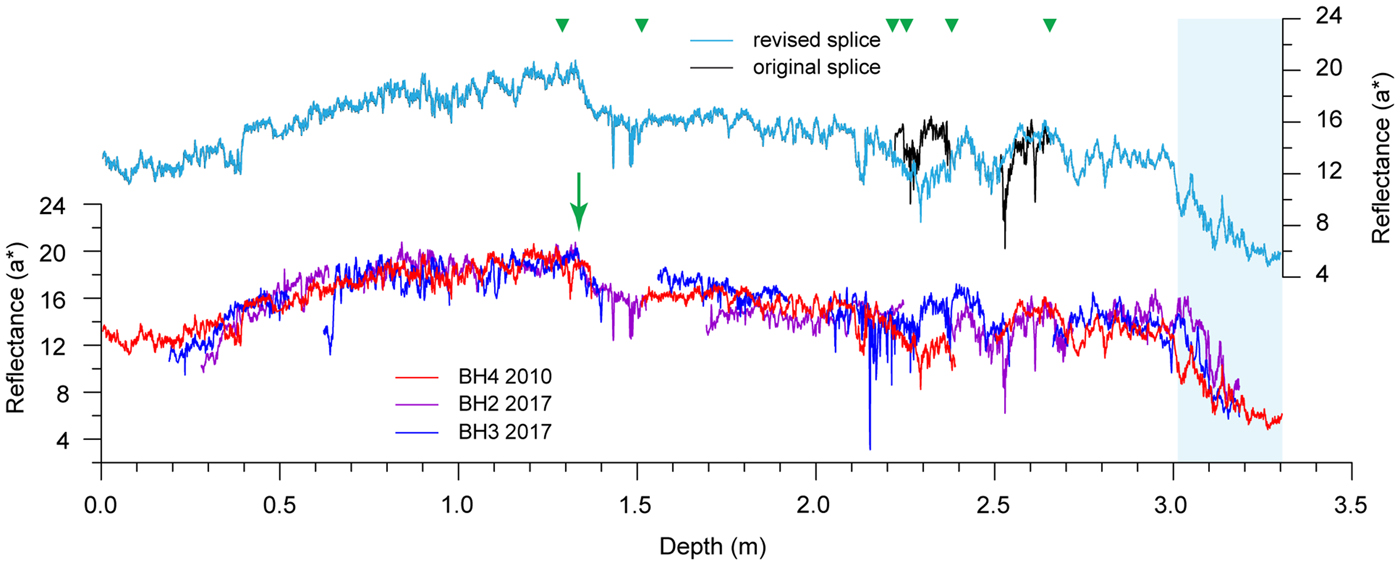
As reflectance data from the three Pegwell Bay cores are discontinuous, composite records for each reflectance parameter were produced using graphic correlation to splice data from the three core data sets (Hagelberg et al., Reference Hagelberg, Pisias, Shackleton, Mix, Harris, Pisias, Mayer, Janecek, Palmer-Julson and van Andel1995). The longest, most continuous core of the three (BH4 2010) was used as the base data set into which data from the other two cores were spliced. Sediment redness—a* reflectance—was selected as the splicing parameter as field observations indicate two distinct color changes (Fig. 1), one within the loess, at approximately 1.35 m depth, and another at the loess/bedrock interface. Both boundaries are denoted by relatively rapid decreases in a* reflectance values (Fig. 6).
Composite a* reflectance record from Pegwell Bay. Green arrow denotes observed change in loess color. Splice points indicated by green triangles. Light-blue box corresponds to the Paleocene bedrock. (For interpretation of the references to color in this figure legend, the reader is referred to the web version of this article.)

Cross correlation
After correcting for nonlinear distortion and scaling effects, we applied a Gaussian interpolation to standardize the number of reflectance data points for the Balkholme Common, Hemingbrough, and Pegwell Bay image data sets. The interpolation interval was determined from the corrected—where applicable—depth interval derived from the standard images as these had the lower resolution. So, for Balkholme Common this is 5 mm, whereas for Hemingbrough and Pegwell it is 16 mm and 10 mm, respectively. Cross correlations between the interpolated reflectance data from the standard and line-scan images were undertaken using Crospec (ARAND software, Brown University) to calculate the best-fit solution using the correlation coefficient (r) and offsets between the two data sets, on the simplest assumption that the best fit would indicate the best or true offset between the two sections. In Crospec, data are normalized before cross correlation is performed. The detrend function in Crospec was not activated, except where specified. Accordingly, all descriptions and interpretations are on undetrended data, unless stated otherwise. A Gaussian interpolation (5 mm intervals, 20mm Gaussian window) was applied to the two Iberian Margin reflectance data sets (U1385 and SHAK06-4K), so that they were broadly comparable to the resolution of the terrestrial data sets mentioned previously.
An important parameter in cross-correlation analysis is the number of lags, or offset iterations, selected. This refers to the number of offset steps from the center by which the sequences are compared; the greater the number of lags, the greater the comparison distance either way (positive or negative) from the zero central offset point. If the sequences are of comparable length, as they are in this study, then as the number of lags increases so there will be a concomitant increased segment at the beginning or end of the displaced sequence that is not being included in the analysis (Supplementary Fig. 5). In this investigation, the iteration interval equates with the interpolation interval. For example, if 120 iterations are applied to a data series with a 5 mm resolution, then the total displacement distance across which a sediment sequence is compared is 600 mm either side (positive or negative) of the zero central offset. Because our reflectance data sets relate to broadly the same sediment, the number of iterations is limited to constrain the best-fit solution around the zero central offset as we are confident the true offset lies close to that.
A further factor to consider before undertaking these cross-correlation analyses is to establish that the images, and hence the reflectance data derived from them, have the same start and end point. For Balkholme Common, where the images are of the same core sections, this is relatively easy to determine. In this example, the sequence extends from the top of the first core to its contact with Triassic bedrock, at 13.7 m depth (Supplementary Fig. 3). For Hemingbrough, the standard image reflectance data were derived from the monoliths photograph (Fig. 2). It is possible here that the end points do not coincide because the trench floor is uneven—the standard image data probably exclude the lowermost 10–15 mm. However, as this is within the overall resolution of the standard image reflectance data, we consider it unlikely to have affected adversely the cross correlation. For Pegwell Bay, the end point was the loess–bedrock contact (Fig. 1). However, ascertaining whether the start points are identical is more problematic because the uppermost 0.4 m in the standard image is obscured by vegetation and the sedimentary sequence is also longer. We acknowledge that the two sequences do not have the same start point, but, as described in the next section, there is a distinctive decalcification horizon identifiable both in the images and reflectance data sets. For the texturally similar marine sediments, the start and end points were determined by depth: the top equated with 0 m depth (top of the first core), and the end point at 4.77 m depth, coincident with the end of the shorter SHAK06-4K core.
Assessing linear trends in the reflectance data
To investigate the potential effect of linear trends on the cross correlation, we undertook two sets of analyses. A linear trend in this context is a uniform-rate change in a parameter, such as color reflectance, along the length of the time/depth series that can be removed by adding or subtracting the constant-rate, linear-fitted slope of the data. Identifying whether data have linear trends is important. This is because these trends could be a natural facet of the data, such as a progressive decrease in L* reflectance signifying decalcification, or an artifact, introduced by variations in ambient lighting up or down a geologic section. Our first set of cross correlations used the undetrended data from the four reflectance data sets. However, as the standard image reflectance data from Hemingbrough indicated an apparent linear trend (discussed in the next section), we detrended this data and ran a second cross-correlation analysis against the respective undetrended line-scan image reflectance data.
Comparing dated and undated reflectance data sets
A critical research objective is to assess the extent to which reflectance data from an undated sequence can be correlated with a chronologically constrained sequence from the same site. From this, we may be able to evaluate the potential for using reflectance parameters to produce preliminary age models. In this study, the marine sediments were used for this comparison as both cores are from the same oceanographic location. Furthermore, these cores were prepared and imaged using identical techniques so any variance in reflectance parameters should represent paleoenvironmental changes rather than differences attributable to other factors, such as ambient lighting. We applied a graphic correlation (Prell et al., Reference Prell, Imbrie, Martinson, Morley, Pisias, Shackleton and Streeter1986) to compare the undated SHAK06-4K reflectance data sets with the U1385 reflectance time series. Of the three published age models for U1385 (Hodell et al., Reference Hodell, Lourens, Crowhurst, Konijnendijk, Tjallingii, Jiménez-Espejo, Skinner and Tzedakis2015), we used the one that correlates the U1385 benthic oxygen isotope record with the LR04 stack of Lisiecki and Raymo (Reference Lisiecki and Raymo2005). Data on elemental composition—specifically Ca/Ti ratios and Zr/Sr ratios—were used to provide an independent assessment of the reflectance correlations. These data were captured using an Avaatech XRF core scanner, sampled respectively at 10 mm and 5 mm intervals for U1385 (Hodell et al., Reference Hodell, Lourens, Crowhurst, Konijnendijk, Tjallingii, Jiménez-Espejo, Skinner and Tzedakis2015) and SHAK06-4K (Channell et al., Reference Channell, Hodell, Crowhurst, Skinner and Muscheler2018). A second graphic correlation was applied to the reflectance and geochemical data sets using the chronological tie points from the southwestern (SW) Iberian Margin JC089 stack (Channell et al., Reference Channell, Hodell, Crowhurst, Skinner and Muscheler2018).
RESULTS
Visual comparisons
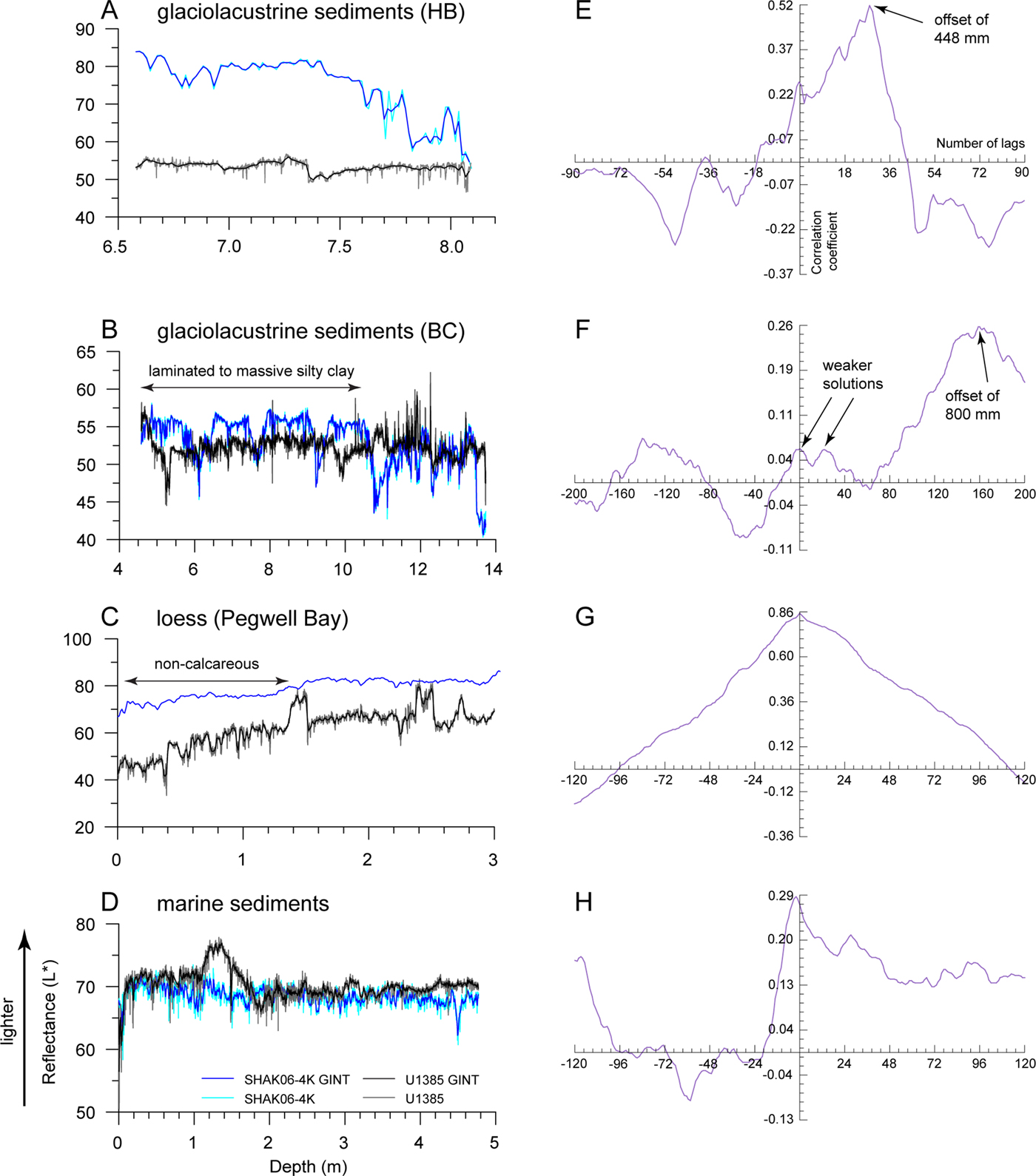
Initial observations of the standard and line-scan image reflectance data indicate significant differences in replicability between the three reflectance parameters at particular sites. First, L* reflectance values—denoting sediment lightness—are consistently numerically higher for the field section standard images (Hemingbrough and Pegwell Bay) (Fig. 7A and C), even where ambient lighting is reduced because of overhanging vegetation or increased shading toward the base of the section (Figs. 1 and 2). The Pegwell Bay standard image data exhibit less variance (standard deviation [SD] = 4.12) than the line-scan counterpart (SD = 8.33) as indicated by a flatter curve. Comparisons of the laboratory-derived data for Balkholme Common, in contrast, indicate that the standard images yield higher L* reflectance values only above 10.5 m depth, where the sediments comprise laminated to massive silty clay (Fig. 7B). Below this depth, the sediments comprise higher proportions of lighter-colored silty sand laminae and beds, which return higher values from the line-scan images.
Comparison between L* reflectance values derived from the standard (blue line) and line-scan images (black line) for glaciolacustrine sediments at Hemingbrough (HB) (A) and Balkholme Common (BC) (B), loess at Pegwell Bay (C), and marine sediments from the Iberian Margin (D). Gaussian interpolated data (GINT) denoted by darker blue or black lines. All data are undetrended. The respective cross correlations for each sedimentary sequence are given in panels E–H. See Supplementary Figure 5 for additional details on how these plots are derived and interpreted. (For interpretation of the references to color in this figure legend, the reader is referred to the web version of this article.)

The extent to which these observed differences can be attributed to the imaging technique can be demonstrated by examining the control reflectance data sets—that is, the Iberian Margin marine sediments (Fig. 7D). For these sediments the L* reflectance values are slightly higher for core U1385, with a prominent peak—denoting much lighter sediment—between 1.2 to 1.8 m depth. This peak, however, is less evident in core SHAK06-4K, an observation consistent with its lower SD value: 1.26, compared with 2.19 for core U1385. Because both core sets were imaged by line scanning, any data variance must represent variations in sediment texture and/or other properties, such as oxidation, moisture content, or percentage of biogenic carbonates. The wider implications of these factors on the L* reflectance signal will be discussed in the next section.
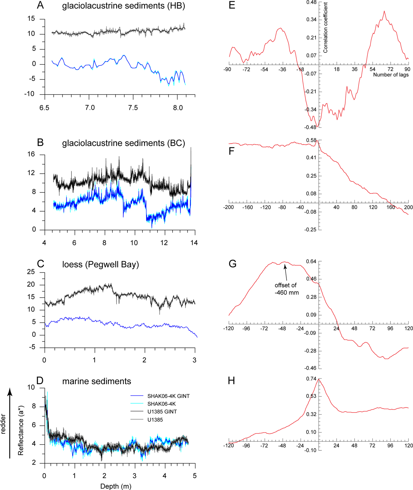
The a* reflectance records—denoting sediment redness—indicate that higher values are derived from the line-scan images (Fig. 8A–C), consistent with the observation that these images appear redder to the naked eye. In detail, differences in reflectance values from the two imaging techniques are most pronounced for Hemingbrough (Fig. 8A). The standard image data indicate an abrupt change at 7.5 m depth, below which the values are consistently lower. This pattern is not replicated in the line-scan image data. For the loess at Pegwell Bay, the standard image reflectance values show significantly less variance (SD = 1.56) than the line-scan image data (SD = 2.34). In particular, the abrupt change in a* reflectance values at 1.3 m depth in the line-scan data is less clearly resolved in the standard image data (Fig. 8C). As expected, the a* reflectance values for the Iberian Margin cores show comparable patterns of change, which is supported by similar SD scores of 0.77 and 0.73 for U1385 and SHAK06-4K, respectively. The most prominent feature, evident in both cores, is the rapid decrease in a* values between 0 and 0.1 m depth (Fig. 8D).
Comparison between a* reflectance values derived from the standard (blue line) and line-scan images (black line) for glaciolacustrine sediments at Hemingbrough (HB) (A) and Balkholme Common (BC) (B), loess at Pegwell Bay (C), and marine sediments from the Iberian Margin (D). Gaussian interpolated data (GINT) denoted by darker blue or black lines. All data are undetrended. The respective cross correlations for each sedimentary sequence are given in panels E–H. See Supplementary Figure 5 for additional details on how these plots are derived and interpreted. (For interpretation of the references to color in this figure legend, the reader is referred to the web version of this article.)

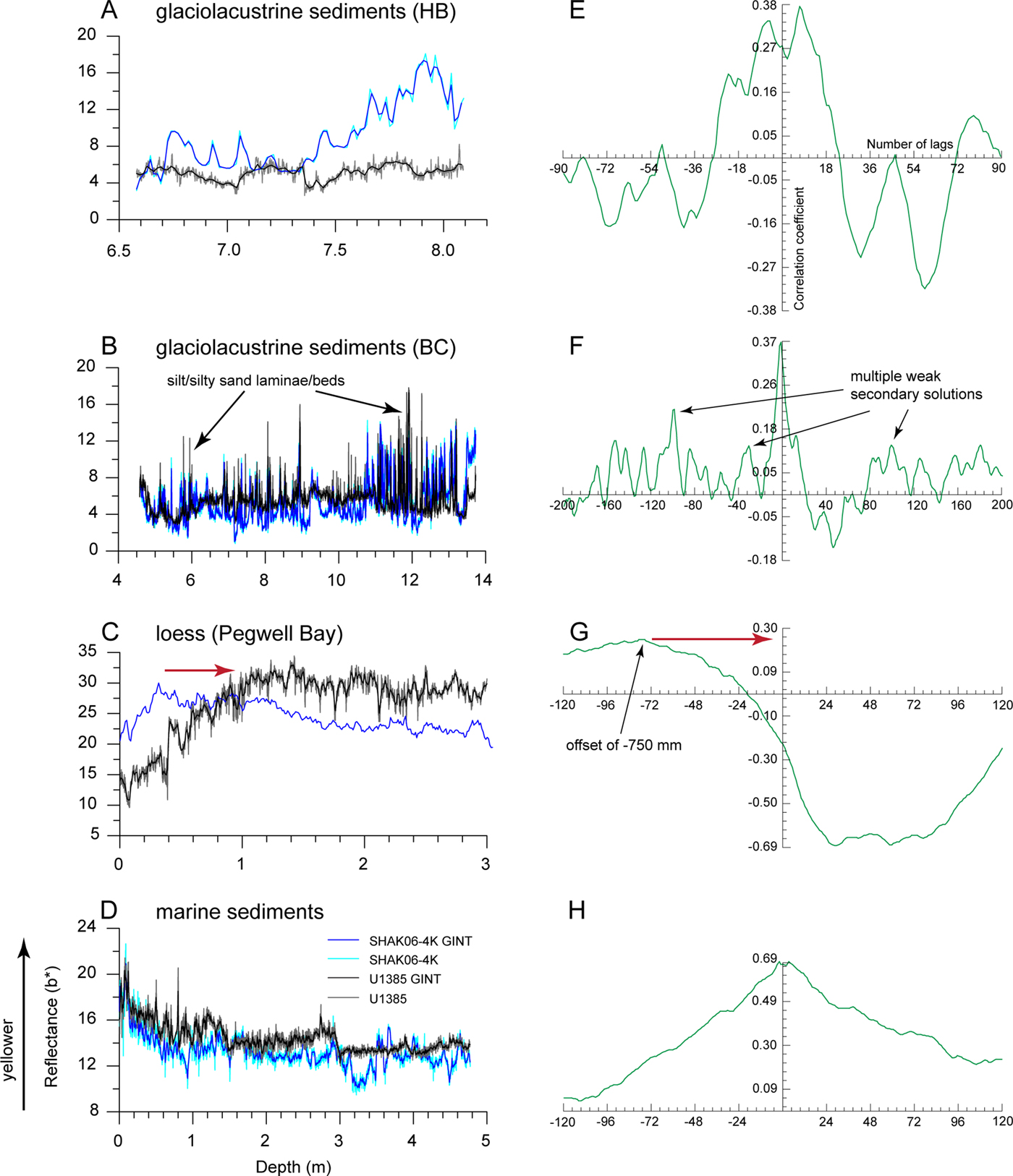
The b* reflectance records—denoting sediment yellowness—show no consistent pattern between data derived from the standard images compared with the line-scan images. In both the Hemingbrough and Balkholme Common records (Fig. 9A–B), there are peaks in b* reflectance values that correspond to yellowish-brown silt or silty sand beds and laminae. However, the Balkholme Common standard images appear more yellowish brown to the naked eye and, therefore, would be expected to return higher b* reflectance values. Despite this, it is the line-scan image data, and in particular those corresponding to the silt or silty sand beds and laminae, that consistently return higher b* reflectance values (Fig. 9B). The standard image record for Hemingbrough also indicates a progressive increase in b* reflectance values below 7.5 m depth, in common with the a* reflectance record described previously. For loess at Pegwell Bay, where the sediments exhibit less textural variation, a key feature is a progressive increase in b* reflectance values downward from the top of the sedimentary sequence (Fig. 9C). In the line-scan data, this increase mainly occurs in the upper 1.0 m, whereas for the standard image data it only occurs in the upper 0.4 m. From the Iberian Margin records, the b* reflectance values are, overall, slightly higher for core U1385 (Fig. 9D).
Comparison between b* reflectance values derived from the standard (blue line) and line-scan images (black line) for glaciolacustrine sediments at Hemingbrough (HB) (A) and Balkholme Common (BC) (B), loess at Pegwell Bay (C), and marine sediments from the Iberian Margin (D). Gaussian interpolated data (GINT) denoted by darker blue or black lines. All data are undetrended. The respective cross correlations for each sedimentary sequence are given in panels E–H. The red arrows denote direction of offset required to produce a best-fit solution at the zero central offset point. See Supplementary Figure 5 for additional details on how these plots are derived and interpreted. (For interpretation of the references to color in this figure legend, the reader is referred to the web version of this article.)

Cross correlation of undetrended data
Comparisons of the standard and line-scan image reflectance data sets highlight potentially significant similarities and differences between the respective records, which we assess using cross-correlation analysis. Focusing first on L* reflectance, the strongest correlation, as indicated by the coefficient score, is produced from the loess records (r = 0.86) (Fig. 7G). The three remaining correlations, in contrast, are much weaker, ranging from 0.52 to 0.26 for the glaciolacustrine sediments (Fig. 7E–F) and 0.29 for the marine sediments (Fig. 7H). Whereas single best-fit solutions with offsets of <5 mm exist for the loess and marine sediments, this is not the case for the glaciolacustrine sediments, where multiple solutions are possible. Offsets from the central zero point for the strongest of these solutions occur respectively at 448 and 800 mm for Hemingbrough and Balkholme Common.
The strength of the a* reflectance correlations varies according to the sedimentary environment. The strongest correlations, with coefficients of 0.74 and 0.64, are produced from the marine sediments and loess, respectively (Fig. 8G–H). Weaker correlations, as indicated by coefficients of 0.58 and 0.29, are produced from the Balkholme Common and Hemingbrough glaciolacustrine sediments, respectively (Fig. 8E–F). Except for the Hemingbrough sediments, all correlations can be resolved with a single best-fit solution. Only the loess has a substantial offset—of 460 mm—from the central zero point. To put this into context, the 460 mm offset is nearly a third of the range (1.2 m) over which the data are compared by the cross-correlation analysis.
The b* reflectance cross correlations are the most variable of all the three reflectance parameters. The strongest correlation (r = 0.69) is associated with the marine sediments (Fig. 9H) where there is a single best-fit solution. The correlations for the glaciolacustrine sediments are much weaker, producing coefficients of just 0.37 or 0.38 (Fig. 9E–F). Multiple peaks in these correlation plots allude to more than one potential solution, although the best-fit solution is always closest to the central zero point. The weakest correlation (r = 0.26) is for the loess, where the offset is −750 mm (Fig. 9G).
Cross correlation of the detrended Hemingbrough data
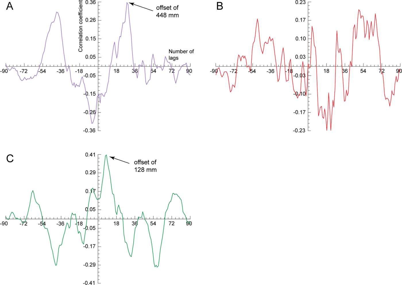
Previous discussion indicates that the standard image reflectance data sets from Hemingbrough are compromised by differences in ambient lighting between the top and bottom of the 1.6-m-high section face. The broadly linear trend of lower L* reflectance values toward the base of the sequence can be removed to a first approximation by detrending the data. The cross correlations for the detrended data indicate multiple solutions for all three reflectance parameters, particularly a* reflectance. Overall, these patterns are similar to the undetrended data. However, in detail, the detrended data correlation coefficients for L* and a* reflectance are lower, at 0.36 and −0.23, respectively, indicating much weaker best-fit solutions (Fig. 10A–B), whereas for b* reflectance, the coefficient is slightly higher, at 0.41 (Fig. 10C). Despite this, the corresponding offsets from the central zero point for these solutions are either identical to the undetrended data, at 448 mm for L* reflectance, or slightly greater, at 128 mm for b* reflectance.
(color online) Cross-correlation plots of L* reflectance (A), a* reflectance (B), and b* reflectance (C) on detrended standard image Hemingbrough reflectance data.

INTERPRETATION AND DISCUSSION
Variations in L* reflectance
As mentioned previously, L* reflectance is a measure of sediment lightness. Because lighting conditions were uniform for the line-scan images, any differences between the reflectance data sets, as indicated by the correlation coefficient and offset from the central zero point, must be because of other factors. We identify three factors likely to have contributed significantly to the differences in L* reflectance records between the standard and line-scan images of the terrestrial sediments: ambient lighting, water content, and textural variations.
Ambient lighting of the standard images is particularly relevant for the field sections where lower L* reflectance values—representing darker sediment—can be attributed to decreasing light levels. The causes of these reductions, at least in this investigation, are site specific. At Pegwell Bay, overhanging vegetation at the top of the section not only introduces shade but also excludes data capture on the standard image where it obscures the field section. Light levels are reduced at Hemingbrough below 7.5 m depth as here the trench section becomes narrower and more confined. Despite these physical constraints, ambient lighting differences alone cannot explain all of the differences between respective L* reflectance data sets because at Pegwell Bay the lowest absolute values are actually recorded in this instance from the line-scan images. Even under more controlled laboratory conditions, such as for the Balkholme Common glaciolacustrine sediments—where lighting levels were constant for the standard images as well— there is no consistent bias toward a particular imaging technique producing higher or lower L* reflectance values.
Physical sedimentary properties such as texture, as well as moisture, organic, or carbonate contents, must also affect the sediment lightness signal in these examples. The wettest sediments were from Balkholme Common, which were imaged immediately after core splitting. As water imparts a surface “glare” to sediments, this may account for the higher standard image L* reflectance values. Yet, despite this, the values are not consistently higher for the standard images, so they also likely represent differences in the water-retaining properties of the constituent minerals, particularly within the clay-sized fraction. Of all the sedimentary environments investigated, the lighter-colored silt to darker-colored silty clay glaciolacustrine sediments exhibit the greatest textural and color variations. It is these differences that may account for the oscillatory pattern between positive and negative correlations on the cross-correlation plot, as well as the multiple weak secondary solutions and the offsets. This is because a match, or solution, would be found repeatedly where configurations of laminated sediments within the core images were similar. For this reason using L* reflectance values from laminated sediments for cross-correlation analysis may be unreliable.
The loessic sediments, on the other hand, show the least textural and color variations. The upper 1.3–1.5 m is noncalcareous (Murton and Giles, Reference Murton and Giles2016) and thus darker than the underlying calcareous loess. However, differences in carbonate content cannot explain why the standard image returns consistently higher L* reflectance values. Possible explanations are that the field-section sediments, captured in the standard image, are drier because of desiccation from sea breezes or have a patina of sea salt, both of which could increase sediment lightness.
Variations in a* reflectance
The factors identified in the previous section also affect a* reflectance values. For this parameter, it is the wetter or less well-illuminated sediments associated with the standard images that consistently return lower values, denoting less red sediment. However, these factors seemingly influence the cross correlations differently, thereby resulting in fewer potential solutions. The negative correlation and secondary solutions for the Hemingbrough glaciolacustrine sediments appear strongly skewed by the antiphase relationship between a* reflectance values below 7.5 m depth. This is likely exacerbated by the shortness of sediment length analyzed, an additional consideration that will be discussed later.
The loess cross correlation differs from the glaciolacustrine correlations in that its best-fit solution has an offset. The field section (Fig. 1) indicates two sedimentary features that may account for this. First, there is a distinct change in sediment redness between 1.3 and 1.5 m depth, coincident with the decalcification horizon identified previously. As both this and the loess–bedrock contact are undulating, it is likely that sedimentation and/or erosion rates differed over time between the two sampled sites, despite being just 45 m apart. In this instance, the offset probably represents the difference in depth where the decalcification horizon occurs in the sedimentary column. This example highlights that the best solution mathematically—with zero offset—is not always the same as the best geologic fit, and that any correlation should be evaluated within its sedimentary context rather than in isolation.
Variations in b* reflectance
The dominant factor influencing the cross correlations between the b* reflectance records is sediment texture. This is most evident in the glaciolacustrine sediments where yellowish brown silty sand beds and laminae correspond with spikes in b* reflectance values. The greater moisture content and lack of core surface preparation for the Balkholme Common standard images seems not to have affected adversely the identification of these textural variations. In common with the L* reflectance cross correlations, these color differences have produced multiple, weak solutions where similar configurations of laminae have been repeatedly identified in the sedimentary sequence. The offset in the loess cross correlation is likely because of the same factors affecting the a* reflectance correlation, discussed previously. Texture exerts less influence on the marine sediment cross correlation because marine sediments are the most homogenous of all the sediments being investigated. In this instance, the strong cross correlation is forced by the sharp peak in b* reflectance values in the upper 0.1 m.
Other considerations
Other potential factors likely to affect the cross correlation are length of sediment being compared and sampling resolution. In this investigation, three of our sedimentary sequences were <5 m long, the shortest being just 1.62 m (Hemingbrough). Of these, only the latter was analyzed over the full data set because of the limited number of data points. Our results indicate that the weakest correlations do not always correspond with the shortest sediment length, or fewest lags, but instead vary according to the reflectance parameter being analyzed. As demonstrated by the b* reflectance correlations for the two glaciolacustrine sediment data sets, where maximum r = 0.37 or 0.38, it makes little difference whether the whole data set is compared (Hemingbrough) or just a narrow central range (Balkholme Common). As discussed previously, it is sediment texture, in particular the yellowish-brown silt laminae, that exerts the strongest control on these correlations.
The sampling resolution used for the correlations was limited to the maximum resolution of the standard images, which differed between sites, because the length of sediment exposed in the field of vision varied. For the Balkholme Common standard images, this was always 1.55 m—the core section length—whereas the field sections photographed at Hemingbrough and Pegwell Bay were longer and contained the entire sedimentary section. Compressing a sedimentary sequence into a single photograph invariably reduces the amount of detail, such as sedimentary structure, that can be captured. This cannot be overcome subsequently by cropping in software such as Photoshop, so as to remove extraneous detail, and then enlarging the region of interest, because the pixel resolution is fixed at the time of original photograph capture when using digital photography. The end result will be blurrier pixels, which compromise data quality. Nonetheless, our data from the glaciolacustrine sediment cross correlations indicate that even though the Hemingbrough data set had fewer data points than the Balkholme Common data set, similar correlation patterns, with multiple secondary solutions for L* and b* reflectance representing patterns in lamination, could still be identified.
Comparing dated and undated reflectance data sets
Our cross correlations for the Iberian Margin data sets indicate that the strongest solution arises from a* reflectance (Fig. 8H) and therefore would likely be the best parameter to use for our initial time series graphic correlation. In this experiment, the correlation is based on aligning data peaks and troughs in the data sets. The best fit of the a* reflectance records was achieved using seven second-order chronological tie points; first-order chronological tie points—in age models—are usually derived from direct dating, such as radiometric dating of foraminifera, or optically stimulated luminescence dating of sandy sediments, and are typically necessary to produce a robust absolute age model. The top of U1385 equated to 0 yr, so we assigned the same age to the top of SHAK06-4K as both cores have relatively high a* reflectance values in the upper 0.1 m, attributable to oxidation close to the sediment–water interface.
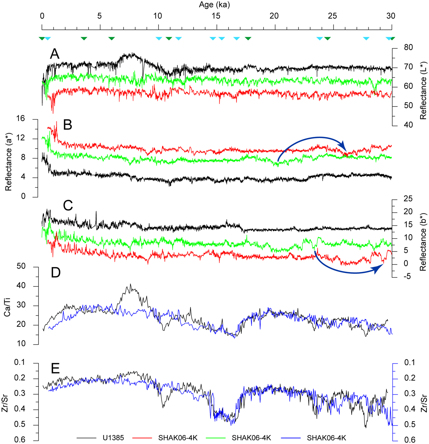
Comparison of the reflectance time series (Fig. 11A–C) indicates that, despite lacking first-order chronological tie points, it is possible to produce a viable yet simple correlation between a dated (U1385) and undated (SHAK06-4K) data set based on variance in a* reflectance. Correlations between the L* and b* reflectance time series in this model, however, are less convincing, with significant deviations in data trends occurring between 7 and 8 ka. This indicates that although the correlation coefficient for b* reflectance is only slightly weaker than for the a* reflectance correlations (0.69 vs. 0.74), there is sufficient variability in the former signal to complicate time series correlations.
Comparison between the time series for L* reflectance (A), a* reflectance (B), and b* reflectance (C) from Iberian Margin cores U1385 (black line) and SHAK06-4K (light-green line). Dark-green triangles denote original chronological tie points imposed on the SHAK06-4K reflectance records and used for the graphic correlation with U1385. Light-blue triangles denote revised chronological tie points from Channell et al. (Reference Channell, Hodell, Crowhurst, Skinner and Muscheler2018) used to correlate the U1385 (black line) and SHAK06-4K (blue line) using Ca/Ti (D) and Zr/Sr (E) ratios. The revised reflectance correlations, using these chronological tie points (light-blue triangles), are indicated by the red lines in panels A–C. Dark-blue arrows highlight examples in age offset resulting from the original (light green) and revised (red) graphic correlations. All SHAK06-4K reflectance parameters are offset from the corresponding U1385 data. (For interpretation of the references to color in this figure legend, the reader is referred to the web version of this article.)

Confidence in the reliability of the a*-reflectance-derived time series is reinforced by comparing the geochemical time series data (Ca/Ti and Zr/Sr ratios) from these two cores. This provides an independent means to verify the chronological tie points underpinning the original graphic correlation because trends in the geochemical data should also be aligned if these points return the best fit. However, applying the SW Iberian Margin JC089 stack chronological tie points does not replicate our initial a*-reflectance-derived time series (Fig. 11). In particular, the revised graphic correlation indicates that our initial correlation consistently underestimates sediment age, even for the uppermost, youngest sediment. This age offset becomes progressively more pronounced down core and is most noticeable in the a* and b* reflectance records (Fig. 11B and C). In part, this underestimation may arise because of an apparent hiatus in sedimentation in SHAK06-4K, corresponding to the Younger Dryas stadial (Channell et al., Reference Channell, Hodell, Crowhurst, Skinner and Muscheler2018). This is observable in the geochemical records by the mismatch between Ca/Ti and Zr/Sr ratios over this interval, but not in the reflectance records. After 13 ka, the geochemical records are more closely aligned.
Criteria for assessing archive photographs
This study illustrates the potential for archive color photographs of terrestrial sediments to be used to extract paleoenvironmental data, even if they do not conform completely to the “best practice” criteria suggested by Zeeden et al. (Reference Zeeden, Krauß, Kels and Lehmkuhl2017). With this in mind, we recommend consideration of six points when assessing archive photographs to extract reflectance data for use in paleoenvironmental reconstructions.
Photographs should have been shot with the same camera and under the same environmental conditions to ensure consistency of a particular data set.
Photographs of field sections are likely to be more plentiful and accessible (through friends, colleagues, and museums) compared with their laboratory counterparts. Our data indicate that data point resolution diminishes significantly with increasing length/depth of sediment photographed. In our examples, we found about 1.5 m to be the optimum depth to capture sediment reflectance variability, with 3 m being the maximum. For longer sedimentary sequences, we suggest overlapping photographs taken at consistent depth intervals and producing a composite depth series by splicing the reflectance data.
Laboratory-derived photographs of sediments taken using mounted digital or analog cameras are generally the least affected by environmental variations, such as lighting. These photographs offer a more reliable means to acquire reflectance data compared with those of field sections. Underutilized photographs of this caliber may reside in unpublished PhD dissertations, national geologic survey repositories, or databases of geotechnical companies.
Both laboratory-derived and field photographs are affected by distortion. This can be corrected providing an accurate measure of real depth, such as a staff or tape measure, is included in the photograph. However, because field sections are nearly always slightly curvilinear, even when carefully cleaned, this introduces additional distortions. The extent to which these distortions affect data quality depends on the purpose for which the reflectance data are intended. Although we do not consider archive photographs to be a substitute for high-resolution line-scan imaging of fresh sediment, the reflectance data captured from them could be useful, for example, as a pilot investigation at a new site. In these instances, distortion is less of a concern if the reflectance data—such as when using a* reflectance to identify paleosols—are compared against similar sediments with comparable accumulation rates from other sites. If, however, the archive photographs are being used to measure thicknesses of laminated (varved) sediment to produce a relative time series, then understanding the degree of distortion is paramount.
Photographs should be of oxidized sediments to ensure variations in the reflectance parameters represent actual paleoenvironmental conditions.
L* reflectance, which is strongly influenced by ambient lighting conditions, is the least reliable of the three reflectance parameters. Paleoenvironmental data are more usefully obtained from a* and b* reflectance, particularly on sediments with significant textural or color variations. This is still possible even at relatively low resolutions.
Criteria for assessing reflectance data from archive photographs
This study demonstrates that, despite the simplicity of capturing reflectance data from archive photographs, the quality of data produced can be highly variable. Based on our post-data-processing routines, we suggest three further points to be considered before interpreting the paleoenvironmental significance of the reflectance data.
Overlay each reflectance data set onto its respective digital photograph, using software such as Adobe Illustrator. Plot this data as a depth series to check that it distinguishes important sedimentary features, such as contacts or structures (Supplementary Fig. 6). If field notes are available, use them to corroborate that all sedimentary features observable in the field have been correctly identified in the reflectance data. Erroneous data points, resulting from edge effects or an unevenly prepared sediment surface, for example, should be deleted from the data set.
Only data that exhibit extraneous linear trends produced by, for example, systematic differences in ambient lighting—as indicated by a progressive increase/decrease in L* reflectance values—should be detrended for comparisons of this sort. If, however, a linear trend can be strongly attributed to other processes, such as decalcification or pedogenesis, then detrending is not required.
The resolution of reflectance data points derived from archive photographs of field sections effectively decreases as sediment length/depth increases. Data from sections between 1.5 and 3.0 m in length may produce a relatively featureless data series, particularly in sediments with limited textural variation.
CONCLUSIONS
Digital images from three contrasting sedimentary environments demonstrate the viability of using archive color photographs for high-resolution color reflectance logging. Of the three constituent CIELAB reflectance parameters, the a* and b* reflectance records are the most consistent between the standard and line-scan images. This study illustrates that archive color photographs of terrestrial sediments may contain significant paleoenvironmental data. Because data acquisition is quick and inexpensive, this method would be useful in the first instance to evaluate the potential for developing high-resolution records of paleoenvironmental change at sites where field exposures are no longer available. This in turn would inform the viability of undertaking new, more substantive investigations at such sites. In addition, reflectance data captured from archive photographs taken repeatedly during recession of field sections can be used to corroborate field observations and to quantify any lithologic variation. In situations where accessing sediment exposures are problematic or unsafe—such as a partially flooded quarry or superficial sediments unconformably overlying bedrock and exposed in coastal cliff sections or in headwalls of permafrost thaw slumps—unmanned aerial vehicles (drones) increasingly provide a viable means to capture high-resolution, georeferenced, digital photographs without needing to correct for distortion. Capturing line-scan images of field sections in this manner is a significant technological advance, particularly if reflectance data are extracted from them and incorporated into paleoenvironmental reconstructions.
More importantly, our data demonstrate the potential for cross-correlation analysis to assist correlation between undated and chronologically constrained sediments. In these analyses, our Crospec-derived correlations are based on linear iterations of the comparison. However, applying more sophisticated correlation techniques, such as Lisiecki's “Match” program (Lisiecki and Lisiecki, Reference Lisiecki and Lisiecki2002), would allow greater flexibility in these comparisons, as the data can be stretched and squeezed to establish the best match. To test this approach, we applied two graphic correlations between undated (SHAK06-4K) and dated (U1385) marine sediments from the Iberian Margin. The best fit was achieved from the a* reflectance time series records. Ca/Ti and Zr/Sr ratio time series records from SHAK06-4K and U1385 were then used to independently verify these a*-reflectance-derived chronological tie points. This demonstrated that the initial match had produced an underestimation of actual sediment age, particularly in sediments older than 13 ka. We attribute this age offset to a hiatus in sedimentation corresponding to the Younger Dryas stadial, which was not identifiable in the reflectance records. These correlations in particular highlight the importance of considering more than one parameter when constructing an age model. Further research is still needed to validate these approaches regarding archive color photographs of terrestrial sediments as all of the featured glaciolacustrine and loess sequences currently lack published high-resolution age models.
SUPPLEMENTARY MATERIAL
The supplementary material for this article can be found at https://doi.org/10.1017/qua.2019.59.
ACKNOWLEDGMENTS
The JC089-SHAK cores used in this study were collected with support from Natural Environment Research Council Grant NE/J00653X/1. The Quaternary Research Association provided financial support for the Pegwell Bay cores. David Hodell and Julian Murton are thanked for respective access to the marine and loess core sections used in this study. Lewis Owen, Matthew Lachniet, Louisa Bradtmiller, Julian Murton, Phil Gibbard, and the anonymous reviewers are thanked for their constructive comments that improved the quality of the manuscript.